Do Identifiability Results for Continuous-Space Extend to Discrete-Space Systems?

Abstract

Researchers develop new models to explain the unknowns. The developed models typically involve parameters that capture tangible quantities, the estimation of which is desired. However, prior to parameter estimation, the identifiability of the parameters should be investigated. Parameter identifiability investigates the recoverability of the unknown parameters given the error-free outputs, inputs, and the developed equations of the model. Different notions of and methods to test identifiability exist for dynamical systems defined in the continuous state space. Yet little attention was paid to identifiability of discrete-space systems, where variables and parameters are defined in a discrete space. We develop the identifiability framework for discrete space systems and highlight that this is not an immediate extension of the continuous space framework. Unlike the continuous case, a “neighborhood” is not uniquely defined in the discrete space, and hence, neither are local identifiability concepts. Moreover, results on algebraic identifiability that proved useful in the continuous space are much less so in their discrete form as the notion of differentiability disappears.

I Introduction

The possibility of uniquely determining the parameters of a dynamical system by observing the inputs and outputs defines the identifiability of that system. This property was investigated in, for example, biology [1, 2, 3], economics [4], epidemiology [5], and control theory [6, 7, 8]. In continuous-space systems, identifiability is defined analytically by output equality, that is whether the equality of two output trajectories implies that of the parameters [9]. In [10], the same idea was formulated as output distinguishability, that is whether two different parameter values result in different output trajectories. A useful technique to investigate the output equality or distinguishability is to use differential algebra, resulting in the notion of algebraic identifiability, that is whether the parameter values can be expressed uniquely in terms of the inputs, outputs, and their time derivatives [3, 11, 12, 13]. A review of both analytical and algebraic identifiability definitions and approaches for continuous space systems under continuous and discrete-time was provided in [14].

Despite the wide application of continuous space systems, there are cases where the state and parameter spaces are restricted to a discrete space. For example, in the context of decision-making dynamics [15], according to the linear threshold model [16, 17] each individual has a unique threshold value and adopts “innovation” (e.g., a new technology) only if the population fraction that has already done so exceeds his threshold. In this system, the output is the number of individuals who have adopted innovation, and the parameter is the distribution of the individuals over the different thresholds. If the parameters of the system are identifiable, the threshold distribution can be determined uniquely and used to simulate and predict the decision dynamics.

There are, however, challenges to extend the existing identifiability concepts and results in the continuous space to the discrete space. Systems defined in discrete spaces lose the useful properties of differentiability. Thus, some available approaches to investigate identifiability based on, for example, the Jacobian matrix, fail in discrete-space systems. Furthermore, in the continuous case, local identifiability notions are not sensitive to how the size and topology of a “neighborhood” are defined. It suffices to show that the system is identifiable in a small enough neighborhood. This is not the case with the discrete case, because the neighborhood of a point cannot be arbitrarily small. Therefore, local identifiability notions depend on how the topology of a neighborhood is defined in the discrete space, and hence, are not uniquely defined.

We aim to extend some available identifiability notions and methods from continuous to discrete-space systems. Our contribution is four-fold: First, we justify the need for a separate framework for the discrete space and explain the subtleties associated with the notion of a discrete neighborhood–Section II. Second, we show that analytical definitions of identifiability, that are based on the output equality approach and generally do not depend on the discrete or continuous nature of the system, can be adjusted to the discrete-space systems with minor changes–Section III. Third, we develop the discrete-space identifiability definitions and show that they are not a ready extension of their continuous-space counterpart, specially those that depend on differentiation, such as the Jacobian, and that they may not be as useful–Section IV. Finally, we show that algebraic and structurally locally identifiability imply each other (Theorem 1) and provide the results that guarantee global identifiability based on the input-output equation–Section V.

II Problem formulation

Consider the discrete-time and discrete-space system

$$\left\{\begin{aligned} &\bm{x}(t+1)=\bm{f}(\bm{x}(t),\bm{u}(t),\bm{\theta}),\quad\bm{x}_{0}=\bm{x}(0)\\ &\bm{y}(t)=\bm{g}(\bm{x}(t),\bm{\theta}),\end{aligned}\right.$$ (1)

where $t\in\mathds{Z}_{\geq 0}$ denotes time, $\bm{x}\in\bm{\mathcal{X}}$, $\bm{u}\in\bm{\mathcal{U}}$, $\bm{y}\in\bm{\mathcal{Y}}$, and $\bm{\theta}\in\mathbf{\Theta}$ are respectively, the vector of states, inputs, outputs, and the parameters, $\bm{\mathcal{X}}\subseteq\mathbb{R}^{\mathtt{x}}$, $\bm{\mathcal{U}}\subseteq\mathbb{R}^{\mathtt{u}}$, $\bm{\mathcal{Y}}\subseteq\mathbb{R}^{\mathtt{y}}$, and $\mathbf{\Theta}\subseteq\mathbb{R}^{\mathtt{\uptheta}}$ are the state, input, output, and parameter space for some positive integers $\mathtt{x},\mathtt{u},\mathtt{y},\mathtt{\uptheta}$, and $\bm{f}:\bm{\mathcal{X}}\to\bm{\mathcal{X}}$ and $\bm{g}:\bm{\mathcal{X}}\to\bm{\mathcal{Y}}$. We assume that the spaces $\bm{\mathcal{X}},\bm{\mathcal{U}},\bm{\mathcal{Y}}$, and $\mathbf{\Theta}$ are uniformly discrete metric spaces, meaning that they each admit some radius $r>0$, such that no two points in the space have a distance of less than $r$ [18]. For example, the discrete spaces can be $\mathbb{Z}^{\mathtt{n}}$ for some positive integer $\mathtt{n}$.

We are interested in the parameter identifiability of system (1). Intuitively, that is whether changes in the parameter values are reflected in the output trajectory. The notion of identifiability is defined both globally and locally. Global identifiability requires the uniqueness of the parameter values in the whole parameter space $\mathbf{\Theta}$ whereas local identifiability shrinks the parameter space of interest into a neighborhood of a parameter $\bm{\theta}\in\mathbf{\Theta}$ [19]. While the notion of a neighborhood is well understood in the continuous-space setting, it is more delicate in the discrete space. Thus, we first present some possible neighborhoods in the discrete space.

II-A Neighborhoods in the discrete space

Any norm can be used to define the distance between points and, subsequently, a neighborhood. For simplicity, we consider the Euclidean norm in the following examples.

Example 1.

Consider the parameter space $\mathds{Z}^{2}$. Perhaps, the simplest neighborhood of a point $\bm{\theta}_{0}\in\mathds{Z}^{2}$ is formed by neighbors that are obtained by moving along any of the basis for one unit from $\bm{\theta}_{0}$. The green circles in Fig. 1(a) illustrate these neighbors for $\bm{\theta}_{0}=\bm{0}$. A wider neighborhood would also include neighbors that are reachable from $\bm{\theta}_{0}$ by moving along two of the basis vectors (the yellow circles). These and other symmetric neighborhoods can be defined by using the notion of a discrete ball with radius $r$, that is the set of all points that lie within the distance of $r$ from $\bm{\theta}_{0}$ denoted by $B(\bm{\theta}_{0},r)=\{\bm{\theta}\in\mathbf{\Theta}\mid\|\bm{\theta}_{0}-\bm{\theta}\|\leq r\}$ (see Fig. 1(a)).

In some applications, the parameter must satisfy certain conditions to be feasible, resulting in a specific structure of the parameter space. For example, should the parameter of interest be a distribution, the parameter space must be a simplex, i.e., the set of non-negative vectors whose entries add up to one.

Example 2.

Consider a population of $n$ decision makers who over time $t=1,2,\ldots$ choose whether to adopt some innovation, e.g., solar panels or augmented reality. Each individual is either a strong coordinator, who decides to adopt if at least half of the population have already done so, or a weak coordinator, who decides to adopt only if at least one third of the population has already done so. The population proportions of strong and week coordinators are unknown and parameterized by $\theta_{1}$ and $\theta_{2}$, respectively, and together by the vector $\bm{\theta}=[\theta_{1},\theta_{2}]^{\top}$. Then, the parameter space is restricted to the simplex $\mathbf{\Theta}=\{\bm{\theta}\in\frac{1}{n}\mathds{Z}^{2}:\theta_{1}+\theta_{2}=1,\theta_{1},\theta_{2}\geq 0\}$. The neighborhood of a point is then restricted to a subset of the simplex. Fig. 1(b) is an example of the parameter space for $n=4$. Then for the parameter value $\bm{\theta}=[\frac{1}{2},\frac{1}{2}]^{\top}$, the neighborhood of radius $\frac{1}{\sqrt{8}}$ would be $B([\frac{1}{2},\frac{1}{2}]^{\top}),\frac{1}{\sqrt{8}})\cap\mathbf{\Theta}$, which consists of the three points $[\frac{3}{4},\frac{1}{4}]^{\top}$, $[\frac{1}{2},\frac{1}{2}]^{\top}$, and $[\frac{1}{4},\frac{3}{4}]^{\top}$. Any symmetric wider neighborhood, e.g., of radius $\frac{1}{\sqrt{2}}$, will match the whole simplex.

(a)

(b)

Figure 1: (a) The neighborhood of $\bm{\theta}_{0}=[0,0]^{\top}$ in $\mathds{Z}^{2}$. $B(\bm{0},2)$ includes all circles, $B(\bm{0},\sqrt{2})$ includes all circles excluding the blue ones, and $B(\bm{0},1)$ includes the green circles and the origin. (b) The one-dimensional simplex intersected with $\frac{1}{4}\mathds{Z}^{2}$. Orange points and the black point form the neighborhood of point $(\frac{1}{2},\frac{1}{2})$ with a radius of $r=\frac{1}{\sqrt{8}}$. The whole simplex can be formulated as $B([\frac{1}{2},\frac{1}{2}]^{\top}),\frac{1}{\sqrt{2}})\cap\mathbf{\Theta}$.

II-B The need for a separate framework

Rather than developing a separate framework for investigating identifiability for discrete-space systems, one may suggest to investigate the identifiability by replacing the discrete function with a continuous function, resulting in a continuous-space system, and then use the already established continuous-space framework and results. The following examples show the inadequacy of this approach. For simplicity, by identifiability here, we refer to the possibility of obtaining a unique value for the parameter of interest. Rigorous definitions are provided in Section III.

Example 3.

Consider the discrete-space system $x(t+1)=-({\theta}-1)^{2}+4$, $y(t)=x(t)$, where $x,y,\theta\in\mathds{Z}_{\geq 0}$. As the system is static, $y(t)$ and $x(t)$ can be written as functions solely dependent on $\theta$. In Fig. 2(a), $y(\theta)$ is shown by black circles and the corresponding continuous replacement $\hat{y}({\theta})$, the output of a similar system where the state, output, and the parameter take values in $\mathbb{R}_{\geq 0}$, is depicted by the blue curve. In the interval $\theta\in(0,3]$, $\hat{y}(\theta)$ is not one-to-one and consequently parameter $\theta$ is not identifiable. However, in the same interval, the discrete function is restricted to $\theta\in\{1,2,3\}$, and hence, $y(\theta)$ is one-to-one. Consequently, $\theta$ is an identifiable parameter for the system in the discrete space.

Example 4.

Consider the discrete-space system $x(t+1)=\sin(\pi\theta)$, $y(t)=x(t)$, where $x,y,\theta\in\mathds{Z}_{\geq 0}$. In Fig. 2(b), $y(\theta)$ is shown by black circles and the corresponding continuous replacement $\hat{y}(\theta)$ is depicted in blue. There is a neighborhood of $\theta=1$ where the continuous function $\hat{y}(\theta)$ is unique yielding the locally identifiability of $\theta$ in the continuous setting. However, in the discrete setting, even for the smallest possible neighborhood of $1$, that is $\{0,1,2\}$, $y(\theta)$ is not one-to-one and consequently parameter $\theta$ is not locally identifiable.

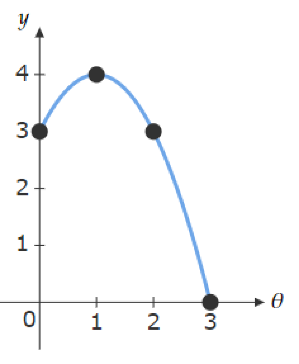
(a)

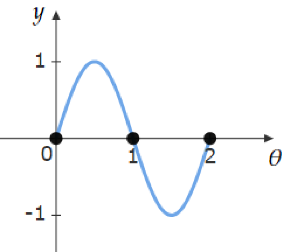
(b)

Figure 2: (a) An example that is not identifiable in continuous space but is in the discrete space. (b) An example that is identifiable in continuous space but not in the discrete space.

Now we proceed to the analytical definitions of identifiability in the discrete-time and space system (1), which are often identical to the of discrete-time and continuous-space case.

III Identifiability: analytical definitions

The main definition of identifiability is based on the equality of the outputs. The idea behind this definition is that, for identifiable parameters, same output trajectories cannot be generated from identical systems that differ only in their parameter values – they must have been generated from the same systems with same parameter values. In other words, a parameter value is identifiable if it is distinguishable from other values, that is, if they result in different output (solution) trajectories [10]. In continuous-time systems, the notion of solution trajectory is defined as the set of pairs $(t,\bm{y}(t))$ for $t\in\mathbb{R}$. In discrete-time systems, one can use the output sequence denoted by $\langle\bm{y}(t)\rangle_{t=0}^{T}$ or simply $\langle\bm{y}(t)\rangle_{0}^{T}$ for some $T>0$. To emphasize the role of the initial condition, input, and parameter in the output, we use the notation $\langle\bm{y}(t,\bm{x}_{0},\langle\bm{u}(t^{\prime})\rangle_{0}^{t-1},\bm{\theta})\rangle_{0}^{T}$ or simply $\langle\bm{y}(t,\bm{x}_{0},\langle\bm{u}(t)\rangle_{0}^{T-1},\bm{\theta})\rangle_{0}^{T}$.

III-A Local identifiability

The notion of locally strongly identifiability was first introduced in [20] for continuous-time and space systems. The following is the equivalent discrete time and space with minor changes, including the initial time being set to $0$ rather than a general $t_{0}$ value. For integer $T>0$, define the set power $\bm{\mathcal{U}}^{T}=\bm{\mathcal{U}}\times\ldots\times\bm{\mathcal{U}}$.

Definition 1.

System (1) is locally strongly $\bm{x}_{0}$-identifiable at $\bm{\theta}\in\mathbf{\Theta}$ if there exists a neighborhood $\mathbf{\Theta}^{\prime}\subset\mathbf{\Theta}$ of $\bm{\theta}$, such that for any $\bm{\theta},\bm{\theta}^{\prime}\in\mathbf{\Theta}^{\prime}$ there is an input sequence $\bm{u}^{*}=\langle\bm{u}(t)\rangle_{0}^{T-1}\in\bm{\mathcal{U}}^{T}$, such that for every time $T>0$,

Remark 1.

The reason why the input sequence $\langle\bm{u}(t)\rangle_{0}^{T-1}$ is up to time $T-1$ only is that in (1) the output is a function of state $\bm{x}(t)$, not the input, and the input $\bm{u}(t)$ determines the value of $\bm{x}(t+1)$. So $\bm{u}(0),\ldots,\bm{u}(T-1)$ together with the initial condition $\bm{x}_{0}$ and parameter $\bm{\theta}$ uniquely determine the output sequence $\langle\bm{y}(t,\bm{x}_{0},\bm{u}^{*},\bm{\theta})\rangle_{0}^{T}$.

Since (2) must hold for any $T>0$ in Definition 1, it must also hold for $T=1$. Moreover, if it holds for $T=1$, then it also holds for any $T>0$. Therefore, Definition 1 can be simplified to the following, implying that the output distinguishability should only be checked for $t=0$ and 1.

Definition 2.

System (1) is locally strongly $\bm{x}_{0}$-identifiable at $\bm{\theta}\in\mathbf{\Theta}$ if there exists a neighborhood $\mathbf{\Theta}^{\prime}\subset\mathbf{\Theta}$ of $\bm{\theta}$, such that for any $\bm{\theta},\bm{\theta}^{\prime}\in\mathbf{\Theta}^{\prime}$ there is an input $\bm{u}(0)\in\bm{\mathcal{U}}$, such that

Remark 2.

The simplification in Definition 2 is merely due to the discrete-time nature of the dynamics, and therefore, also applies to discrete-time continuous-space systems. This definition is restrictive since the dimension of the parameter space can be at most two times the dimension of the output, i.e., $\mathtt{\uptheta}\leq 2\mathtt{y}$ in order for the system to be identifiable. This motivates the less restrictive Definition 3.

Definition 3 ([21, 14]).

System (1) is locally strongly $\bm{x}_{0}$-identifiable at $\bm{\theta}\in\mathbf{\Theta}$ through the input sequence $\bm{u}^{*}=\langle\bm{u}(t)\rangle_{t=0}^{T-1}\in\bm{\mathcal{U}}^{T}$ for some $T>0$, if there exists a neighborhood $\mathbf{\Theta}^{\prime}\subset\mathbf{\Theta}$ of $\bm{\theta}$, such that for any $\bm{\theta},\bm{\theta}^{\prime}\in\mathbf{\Theta}^{\prime}$,

Definition 2 (and equivalently Definition 1) is constrained in several aspects. First, it is about identifiability at a certain initial condition $\bm{x}_{0}$. The following example shows how a system can be identifiable only at some initial conditions. It also highlights the role of the neighborhood.

Example 5.

Consider the discrete-time and discrete-space system defined by $x(t+1)=\theta^{2}x(t)$ and $y(t)=x(t)$, where $x,y,\theta\in\mathds{Z}$. For $x_{0}=0$, $\theta\neq\theta^{\prime}$ does not imply $y(t,x,\theta)\neq y(t,x,\theta^{\prime})$. Therefore, for all $\theta\in{\Theta}$, the system is not locally strongly $0$-identifiable at $\theta$. Nevertheless, for all other $x_{0}\neq 0$, the systems is locally strongly $x_{0}$-identifiable at any $\theta\neq 0$. The neighborhood that makes (2) satisfied is $B(\theta,1)$, i.e., the only case where two different $\theta$ and $\theta^{\prime}$ can result in the same output trajectory is when $\theta=-\theta^{\prime}$; however, the two then do not lie in the same ball $B(\theta,1)$ for $\theta\neq 0$. The same is not concluded for the neighborhood $B(\theta,2)$ as then for $\theta=1$, the ball includes the non-distinguishable parameter values $1$ and $-1$.

III-B Local structural identifiability

The notion of locally strongly $\bm{x}_{0}$-identifiability defined in Definition 2 is for a given $\bm{x}_{0}$. If the system is strongly locally $\bm{x}_{0}$-identifiable for every initial condition $\bm{x}_{0}$ in the state space, then we say that the system is structurally identifiable [22, 12, 14]. It additionally requires the existence of some input space $\bm{\mathcal{U}}^{T}$ such that the system is strongly locally $\bm{x}_{0}$-identifiable for every input sequence in $\bm{\mathcal{U}}^{T}$. A weak notion of structural identifiability was presented in [19, 21] where instead of the whole state space, it requires identifiability for initial conditions in some subset of the state space only.

Definition 4.

System (1) is locally structurally identifiable if there exist a $T>0$ and subsets $\mathbf{\Theta}^{\prime}\subseteq\mathbf{\Theta}$, $\bm{\mathcal{X}}^{\prime}\subseteq\bm{\mathcal{X}}$, and $\bm{\mathcal{U}}^{\prime}\subseteq\bm{\mathcal{U}}^{T}$, such that the system is locally strongly $\bm{x}_{0}$-identifiable at $\bm{\theta}$ through the input sequence $\langle\bm{u}(t)\rangle_{0}^{T-1}$ for every $\bm{\theta}\in\mathbf{\Theta}^{\prime}$, $\bm{x}_{0}\in\bm{\mathcal{X}}^{\prime}$, and $\langle\bm{u}(t)\rangle_{0}^{T-1}\in\bm{\mathcal{U}}^{\prime}$.

Example 6.

The system in Example 5 is structurally identifiable for the sets $\mathcal{X}^{\prime}=\mathds{Z}\backslash\{0\}$ and ${\Theta^{\prime}}={\Theta}$.

III-C Global identifiability

Definition 5 ([12]).

System (1) is globally identifiable at $\bm{\theta}$ if there exist a $T>0$ and an input sequence $\bm{u}^{*}=\langle\bm{u}(t)\rangle_{0}^{T-1}$ such that for almost all $\bm{\theta}^{\prime}\in\mathbf{\Theta}$ and all $\bm{x}_{0}\in\bm{\mathcal{X}}$,

$$\langle y(t,\bm{x}_{0},\bm{u}^{*},\bm{\theta}^{\prime})\rangle_{0}^{T}=\langle y(t,\bm{x}_{0},\bm{u}^{*},\bm{\theta})\rangle_{0}^{T}\Rightarrow\bm{\theta}^{\prime}=\bm{\theta}.$$ (5)

Remark 3.

The identifiability of the system is considered in all the definitions we presented so far. That is, each component $\theta_{i}$ of $\bm{\theta}$ where $i\in\{1,\dots,\mathtt{\uptheta}\}$ is identifiable. However, it is possible to check the identifiability of one component $\theta_{i}$ of interest using the same definitions.

IV Identifiability: algebraic definitions

In analytic definitions, we infer about the equality of the parameter values using the equality of the corresponding two output trajectories. The notion of algebraic identifiability instead is based on constructing the so-called input-output equation, also referred to as the algebraic equation, in the form of $\bm{\Phi}=0$, where $\bm{\Phi}$ equations consisting of the parameters and time iterations of inputs and outputs. Then, the possibility of solving the input-output equation to uniquely determine the parameter values is investigated.

IV-A Definitions

The main component of the algebraic identifiability definition is the existence of the algebraic equation. However, in order for the equation to have a solution for the parameter, at least locally, different assumptions are made. In the original definition [23], which was for continuous-time systems, the parameter was supposed to be algebraic over the differential field of the input and output, which implies that $\bm{\Phi}$ is a polynomial of the input and output and their (higher-order) derivatives and the parameter. In some later work [21, 24], both for continuous and discrete-time systems, a different assumption was made to enforce the existence of solution: the Jacobian of the function $\bm{\Phi}$ with respect to the parameters is supposed non-singular, at least locally. This second definition is particularly useful when the input-output equation is not algebraic (polynomial); then by checking the Jacobian , which is often straightforward, identifiability is verified.

However, neither a differential field nor the Jacobian are defined in the discrete space. One can use the equivalence difference field instead of the differential field, resulting in an almost identical definition of algebraic identifiability in the discrete space. However, for the Jacobian matrix, the extension is not as straightforward.

IV-B Algebraic identifiability based on the difference field

We first present a difference field [25] that is the equivalence discrete-time version of a differential field [23, 14].

Definition 6 ([25]).

A difference field $K$ is a pair consisting of a commutative field $k$ and an automorphism $\delta:k\to k$ such that for all $a,b\in k$, it holds, $\delta(a+b)=\delta(a)+\delta(b)$ and $\delta(ab)=\delta(a)\delta(b)$.

Let $q$ be the shift operator, defined as $q^{T}\bm{h}(t)=\bm{h}(t-T)$ for any function $\bm{h}:\mathds{R}\to\mathds{R}^{\mathtt{n}},\mathtt{n}\in\mathds{Z}_{>0}$, where $T\in\mathds{Z}_{>0}$.

Definition 7.

A shift-operator (difference-)field $K$ is a difference field with the shift operator as the automorphism.

The notation $K\langle\bm{h}(t)\rangle$ or simply $K\langle\bm{h}\rangle$ is a polynomial ring, consisting of all polynomials of $\bm{h}(t)$ with coefficients from the field $K$. If $K$ is a shift-operator difference field, then the coefficients can turn $\bm{h}(t)$ to $\bm{h}(t-1),\bm{h}(t-2),\ldots$. As a result, $K\langle\bm{h}(t)\rangle$ would include polynomials of $\bm{h}(t),\bm{h}(t-1),\ldots$.

Definition 8.

Let $K$ be a shift-operator difference-field. System (1) is algebraically identifiable if $\bm{\theta}$ is (transformally) algebraic over $K\langle\bm{u},\bm{y}\rangle$.

Definition 8 means that $\bm{\theta}$ satisfies a non-zero polynomial $\bm{\Phi}$ of itself and $\bm{u}(t)$ and $\bm{y}(t)$ and their iterates:

$$\bm{\Phi}(\bm{\theta},\langle\bm{u}(t)\rangle_{0}^{T-1},\langle\bm{y}(t,\langle\bm{u}(s)\rangle_{0}^{t-1},\bm{\theta})\rangle_{0}^{T})=\bm{0}$$ (6)

for some $T>0$. Similar to the continuous case, the fact that $\bm{\Phi}$ is a polynomial, guarantees that there are a finite number of solutions for $\bm{\theta}$, and hence, it is locally identifiable.

Remark 4.

Definition 8 also works for discrete-time continuous-space systems.

Remark 5.

The fact that (6) holds, implies that there is a valid $\bm{\theta}\in\bm{\Theta}$ that is a solution to the equation.

IV-C Algebraic identifiability using discrete Jacobian

We define a discrete Jacobian matrix based on finite differences. Given vector $\bm{X}\in\mathds{R}^{\mathtt{n}}$, its $i^{\text{th}}$ entry is denoted by $X_{i}$. (1).

Definition 9 (Forward finite difference).

Given the scalar function $\Phi:\bm{\mathcal{D}}\to\mathds{R},\bm{\mathcal{D}}\subseteq\mathds{R}^{\mathtt{n}},\mathtt{n}\in\mathds{Z}_{\geq 1},$ the forward finite difference along $\mathtt{j}$ by $r$ units at $\bm{\theta}\in\bm{\mathcal{D}}$, where $\mathtt{j}\in\{\mathtt{1},\ldots,\mathtt{n}\}$ and $r$ is such that $\bm{\theta}+r\bm{e}_{\mathtt{j}}\in\bm{\mathcal{D}}$, is defined by

$$\Delta^{r,\mathtt{j}}\Phi(\bm{\theta})\triangleq\Phi(\bm{\theta}+r\bm{e}_{\mathtt{j}})-\Phi(\bm{\theta})$$

where $\bm{e}_{\mathtt{j}}$ is the $\mathtt{j}^{\text{th}}$ column of the $n\times n$ identity matrix.

Definition 10 (Discrete Jacobian).

Given function $\bm{\Phi}:\bm{\mathcal{D}}\to\mathds{R}^{\mathtt{m}},\bm{\mathcal{D}}\subseteq\mathds{R}^{\mathtt{\uptheta}},\mathtt{m},\mathtt{\uptheta}\in\mathds{Z}_{\geq 1},$ point $\bm{\theta}\in\bm{\mathcal{D}}$, and vector $\bm{r}\in\mathds{R}^{\mathtt{\uptheta}}$ satisfying $\bm{\theta}+\bm{r}\in\bm{\mathcal{D}}$, the discrete Jacobian of $\bm{\Phi}$ by $\bm{r}$ with respect to $\bm{\theta}$ is defined by

$$\Delta^{\bm{r}}\bm{\Phi}(\bm{\theta})\triangleq\begin{bmatrix}\Delta^{r_{\mathtt{1}},\mathtt{1}}\Phi_{\mathtt{1}}(\bm{\theta})&\dots&\Delta^{r_{\mathtt{\uptheta}},\mathtt{\uptheta}}\Phi_{1}(\bm{\theta})\\ \vdots&\ddots&\vdots\\ \Delta^{r_{\mathtt{1}},\mathtt{1}}\Phi_{\mathtt{m}}(\bm{\theta})&\dots&\Delta^{r_{\mathtt{\uptheta}},\mathtt{\uptheta}}\Phi_{\mathtt{m}}(\bm{\theta})\\ \end{bmatrix}.$$

Equivalently, the Jacobian can be written as

$$\Delta^{\bm{r}}\bm{\Phi}(\bm{\theta})=[\bm{\Phi}(\bm{\theta}+r_{\mathtt{1}}\bm{e}_{\mathtt{1}}),\ldots,\bm{\Phi}(\bm{\theta}+r_{\mathtt{\uptheta}}\bm{e}_{\mathtt{\uptheta}})]-[\bm{\Phi}(\bm{\theta}),\ldots,\bm{\Phi}(\bm{\theta})].$$

Similar to continuous-space Jacobian, the discrete Jacobian can be applied to a multivariate function. Then the notation $\Delta^{\bm{r}}_{\bm{\theta}}$ is used to indicate that the Jacobian is applied with respect to the variable $\bm{\theta}$.

Example 7.

Let $\bm{\theta}\in\mathds{Z}^{2}$, $y\in\mathds{Z}$, and $\bm{\Phi}(\bm{\theta},y)=[\theta_{1}\theta_{2},\theta_{1}^{2}+\theta_{2}y]^{\top}$. Then for $\bm{r}\in\mathds{Z}^{2}$,

$$\Delta^{\bm{r}}_{\bm{\theta}}\bm{\Phi}(\bm{\theta},y)=\begin{bmatrix}r_{1}\theta_{2}&r_{2}\theta_{1}\\ 2r_{1}\theta_{1}+r_{1}^{2}&r_{2}y\\ \end{bmatrix}.$$

The reason for having a non-singular Jacobian in the definition of algebraic identifiability in the continuous case is to use the Implicit Function Theorem, guaranteeing the local injectivity of $\bm{\Phi}$ and in turn the possibility of obtaining a locally unique value of $\bm{\theta}$ from the equation $\bm{\Phi}=\bm{0}$. The idea is that for arbitrary points $\bm{\theta}^{\prime}$ in a small enough neighborhood of some reference point $\bm{\theta}=\bm{0}$, where the Jacobian is non-singular, Taylor’s expansion can be used to approximate $\bm{\Phi}(\bm{\theta}^{\prime})$ as $\bm{\Phi}(\bm{0})$ plus the Jacobian times $\bm{\theta}^{\prime}$, and by taking the inverse of the Jacobian, $\bm{\theta}^{\prime}$ can be written in terms of $\bm{\Phi}(\bm{\theta}^{\prime})$, implying one-to-oneness in that neighborhood.

In the discrete space, however, there is no “small enough” neighborhood. There is a minimum distance between every two points. Therefore, the higher order terms in Taylor’s expansion can generally not be ignored, because the neighborhood may not be small enough. Nevertheless, if $\bm{\Phi}$ is separable, then we can write $\bm{\Phi}(\bm{\theta}^{\prime})$ in exact terms of $\bm{\Phi}(\bm{\theta})$ for an arbitrary $\bm{\theta}$, which can result in the injectivity of $\bm{\Phi}$ as stated in Lemma 1. In what follows, let $\bm{0}$ (resp. $\bm{1}$) be the all-zero (resp. one) vector with an appropriate dimension.

Definition 11 ([26]).

Function $\bm{\Phi}:\bm{\mathcal{D}}\to\mathds{R}^{\mathtt{m}},\bm{\mathcal{D}}\subseteq\mathds{R}^{\mathtt{\uptheta}},\mathtt{m},\mathtt{\uptheta}\in\mathds{Z}_{\geq 1},$ is (additively) separable if there exist $\mathtt{\uptheta}$ functions $\bm{g}_{i}:\mathds{R}\to\mathds{R}^{\mathtt{m}}$, $i=\mathtt{1},\ldots,\mathtt{\uptheta}$, such that $\bm{\Phi}(\bm{\theta})=\sum_{i=\mathtt{1}}^{\mathtt{\uptheta}}\bm{g}_{i}(\theta_{i})$ for all $\bm{\theta}\in\bm{\mathcal{D}}$.

Lemma 1.

Consider an additively separable function $\Phi:\bm{\mathcal{D}}\to\mathds{R}^{\mathtt{m}},\bm{\mathcal{D}}\subseteq\mathds{R}^{\mathtt{\uptheta}},\mathtt{m},\mathtt{\uptheta}\in\mathds{Z}_{\geq 1}$. For all $\bm{\theta}\in\bm{\mathcal{D}}$ and $\bm{r}\in\mathds{R}^{\mathtt{\uptheta}}\setminus\{\bm{0}\}$ satisfying $\bm{\theta}+\bm{r}\in\bm{\mathcal{D}}$, $\Delta^{\bm{r}}\bm{\Phi}(\bm{\theta})\bm{1}\neq\bm{0}$ if and only if $\bm{\Phi}$ is one-to-one on $\bm{\mathcal{D}}$.

See the Appendix for the proof. The following example highlights the necessity that the function is separable in order for it to be injective.

Example 8.

Take $\phi(\theta_{1},\theta_{2})=\theta_{1}\theta_{2}$ which is not additively separable. Then $\Delta^{\bm{1}}\phi\bm{1}=\theta_{1}+\theta_{2}$ and $\Delta^{\bm{1}}\phi\bm{1}\neq 0$ when $\theta_{1}\neq-\theta_{2}$. However, for $(\theta_{1},\theta_{2})\in\{(a,\frac{1}{a}):a\neq 0\}$, $\phi(\theta_{1},\theta_{2})=1$ implying $\phi$ is not one-to-one. Thus, when $\phi$ is not additively separable, $\Delta^{\bm{1}}\phi\bm{1}\neq 0$ does not necessarily imply that $\phi$ is one-to-one.

Using the discrete Jacobian, we provide the discrete version of algebraic identifiability defined in [21][Definition 5].

Definition 12.

System (1) is algebraically identifiable if there exist a positive integer $T$, subsets $\bm{\mathcal{U}}^{\prime}\subset\bm{\mathcal{U}}^{T}$, $\mathbf{\Theta}^{\prime}\subset\mathbf{\Theta}$, and an additively separable function $\bm{\Phi}:\bm{\Theta}\times\bm{\mathcal{U}}^{\prime}\times\bm{\mathcal{Y}}^{T+1}\rightarrow\mathds{R}^{\mathtt{\uptheta}}$ with respect to its first argument, such that

$$\bm{\Phi}(\bm{\theta},\bm{u}^{*},\langle\bm{y}(t,\bm{u}^{*},\bm{\theta})\rangle_{0}^{T})=\bm{0},$$ (7)

$$\Delta^{\bm{r}}_{\bm{\theta}}\bm{\Phi}\bm{1}\neq\bm{0}$$ (8)

for all $(\bm{\theta},\bm{u}^{*})\in\bm{\Theta}^{\prime}\times\bm{\mathcal{U}}^{\prime}$ where $\bm{u}^{*}=\langle\bm{u}(t)\rangle_{0}^{T-1}$, and for all $\bm{r}\in\mathds{R}^{\mathtt{\uptheta}}\setminus\{\bm{0}\}$ satisfying $\bm{\theta}+\bm{r}\in\mathbf{\Theta}^{\prime}$.

The separability condition on $\bm{\Phi}$ means that $\bm{\Phi}(\bm{\theta},\cdot,\cdot)$ is additively separable with respect to $\bm{\theta}$.

Example 9.

For $u(t)\in\mathds{R}_{>0}$, $y\in\mathds{R}$, and $\bm{\theta}\in\mathds{Z}_{\geq 0}^{2}$, define the separable function $\bm{\Phi}(\bm{\theta},u(0),\langle y(t,u(0),\bm{\theta})\rangle_{0}^{1})=[\theta_{2}u(0),\theta_{1}^{2}u(0)+y(1)]^{\top}.$ By simplifying the notations $\langle y(t,u(0),\bm{\theta})\rangle_{0}^{1}$ to $\langle y(t)\rangle_{0}^{1}$ and $u(0)$ to $u_{0}$, we have

$$\Delta^{\bm{r}}_{\bm{\theta}}\bm{\Phi}(\bm{\theta},u_{0},\langle y(t)\rangle_{0}^{1})=\begin{bmatrix}0&r_{2}u_{0}\\ (2\theta_{1}+r_{1})r_{1}u_{0}&0\\ \end{bmatrix}.$$

Hence, $\bm{\Phi}$ is one-to-one if and only if $\Delta^{\bm{r}}_{\bm{\theta}}\bm{\Phi}\bm{1}\neq\bm{0}$ for all $\bm{r}\neq\bm{0}$, or equivalently

$$[r_{2}u_{0},(2\theta_{1}+r_{1})r_{1}u_{0}]^{\top}\neq\bm{0}.$$ (9)

On the other hand, if we were to check whether $\bm{\Phi}$ is one-to-one by using the definition of injective functions, we would verify the following for a nonzero $\bm{r}$:

$$\bm{\Phi}(\bm{\theta},u_{0},\langle y(t)\rangle_{0}^{1}) \neq\bm{\Phi}(\bm{\theta}+\bm{r},u_{0},\langle y(t)\rangle_{0}^{1})$$

$$[\theta_{2}u_{0},\theta_{1}^{2}u_{0}+y(1)]^{\top} \neq[(\theta_{2}+r_{2})u_{0},(\theta_{1}+r_{1})^{2}u_{0}+y(1)]^{\top}$$

which results in again (9). Therefore, the approach of using the Jacobian for verifying one-to-oneness requires the same, if not more, computational effort compared to the second, original approach.

Example 9 illustrates that applying the Jacobian approach in Definition 12 for identifiability may not be of great use. Moreover, Definition 12 can be applied only to additively separable functions. These caveats motivates us to provide the following third definition of algebraic identifiability.

IV-D Algebraic identifiability based on injectivity

Definition 13.

System (1) is algebraically identifiable if there exist a positive integer $T$, subsets $\bm{\mathcal{U}}^{\prime}\subset\bm{\mathcal{U}}^{T}$, $\mathbf{\Theta}^{\prime}\subset\mathbf{\Theta}$, and a function $\bm{\Phi}:\bm{\Theta}\times\bm{\mathcal{U}}^{\prime}\times\bm{\mathcal{Y}}^{T+1}\rightarrow\mathds{R}^{\mathtt{\uptheta}}$ such that for all $(\bm{\theta},\bm{u}^{*})\in\mathbf{\Theta}^{\prime}\times\bm{\mathcal{U}}^{\prime}$,

$$\bm{\Phi}(\bm{\theta},\bm{u}^{*},\langle\bm{y}(t,\bm{u}^{*},\bm{\theta})\rangle_{0}^{T})=\bm{0}$$ (10)

and for all $(\bm{u}^{*},\bm{y}^{*})\in\bm{\mathcal{U}}^{\prime}\times\bm{\mathcal{Y}}^{T+1}$,

$$\bm{\Phi}(\cdot,\bm{u}^{*},\bm{y}^{*})\text{ is one-to-one in }\bm{\Theta}^{\prime}.$$ (11)

The one-to-one condition, Eq. 11, guarantees the existence of a unique inverse function that allows to obtain $\bm{\theta}$ in terms of inputs and outputs and their iterates.

Remark 6.

If the initial conditions are known, they may provide additional information to retrieve the parameters. Then Definitions 12 and 13 change to the so-called algebraic identifiability with known initial conditions [21], resulting in Definitions 14 and 15.

Remark 7.

Definition 8 implies Definition 12, but no vice versa because Definition 8 requires $\bm{\Phi}$ to be a polynomial. Moreover, in view of Lemma 1, Definition 12 implies Definition 13, but not vice versa, because $\bm{\Phi}$ in Definition 13 does not need to be separable.

V Results

V-A Local result

The following theorem links the notion of algebraic identifiability with that of local structural identifiability.

Theorem 1.

System (1) is locally structurally identifiable iff it is algebraically identifiable with known initial conditions (defined by Definition 15).

Proof:

(sufficiency) Since the system is structurally identifiable, there exists a time $T>0$ and subsets $\mathbf{\Theta}^{\prime}\subseteq\mathbf{\Theta}$, $\bm{\mathcal{X}}^{\prime}\subseteq\bm{\mathcal{X}}$, and $\bm{\mathcal{U}}^{\prime}\subseteq\bm{\mathcal{U}}^{T}$, such that the outputs of any distinct $\bm{\theta},\bm{\theta}^{\prime}\in\mathbf{\Theta}^{\prime}$ are different at time $T$, i.e., $\bm{y}(\bm{f}^{T}(\bm{x}_{0},\bm{u}(0),\dots,\bm{u}(T-1)),\bm{\theta})\neq\bm{y}(\bm{f}^{T}(\bm{x}_{0},\bm{u}(0),\dots,\bm{u}(T-1)),\bm{\theta}^{\prime})$, for every initial condition $\bm{x}_{0}\in\bm{\mathcal{X}}^{\prime}$ and input sequence $\langle\bm{u}(t)\rangle_{0}^{T-1}\in\bm{\mathcal{U}}^{\prime}$. Thus, function $\bm{\Psi}:\mathbf{\Theta}^{\prime}\times\bm{\mathcal{X}}^{\prime}\times\bm{\mathcal{U}}^{\prime}\to\bm{\mathcal{Y}}^{T+1}$ defined by

$$\bm{\Psi}(\bm{\theta},\bm{x}_{0},\langle\bm{u}(t)\rangle_{0}^{T-1})=\begin{bmatrix}\bm{y}(\bm{x}_{0},\bm{\theta})\\ \bm{y}(\bm{f}(\bm{x}_{0},\bm{u}(0)),\bm{\theta})\\ \vdots\\ \bm{y}(\bm{f}^{T}(\bm{x}_{0},\bm{u}(0),\dots,\bm{u}(T-1)),\bm{\theta})\end{bmatrix}$$

is one-to-one with respect to $\bm{\theta}$ in $\bm{\Theta}^{\prime}$. Hence, the inverse function $\bm{\Psi}^{-1}:\bm{\mathcal{X}}\times\bm{\mathcal{U}}^{\prime}\times\bm{\mathcal{Y}}^{T+1}\to\bm{\Theta}^{\prime}$ exists, where $\bm{\Psi}^{-1}(\bm{x}_{0},\bm{u}^{*},\bm{y}^{*})=\bm{\theta}$ for $\bm{y}^{*}=\langle\bm{y}(t,\bm{u}^{*},\bm{\theta})\rangle_{0}^{T}$ where $\bm{u}^{*}=\langle\bm{u}(t)\rangle_{0}^{T-1}$ and $\bm{y}^{*}=\langle\bm{y}(t)\rangle_{0}^{T}$. Now consider the function $\bm{\Phi}:\bm{\Theta}\times\bm{\mathcal{X}}\times\bm{\mathcal{U}}^{\prime}\times\bm{\mathcal{Y}}^{T+1}\rightarrow\mathds{R}^{\mathtt{\uptheta}}$ defined by

$$\bm{\Phi}(\bm{\theta},\bm{x}_{0},\bm{u}^{*},\bm{y}^{*})=\bm{\theta}-\bm{\Psi}^{-1}(\bm{x}_{0},\bm{u}^{*},\bm{y}^{*}).$$

Clearly, (16) is satisfied when $\bm{y}^{*}$ satisfies the dynamics of System (1). On the other hand, $\bm{\Phi}$ is one-to-one with respect to $\bm{\theta}$, because for distinct $\bm{\theta},\bm{\theta}^{\prime}\in\bm{\Theta}^{\prime}$, the equality $\bm{\theta}-\bm{\Psi}^{-1}(\bm{x}_{0},\bm{u}^{*},\bm{y}^{*})=\bm{\theta}^{\prime}-\bm{\Psi}^{-1}(\bm{x}_{0},\bm{u}^{*},\bm{y}^{*})$ implies $\bm{\theta}=\bm{\theta}^{\prime}$ for all $(\bm{x}_{0},\bm{u}^{*},\bm{y}^{*})\in\bm{\mathcal{X}}\times\bm{\mathcal{U}}^{\prime}\times\bm{\mathcal{Y}}^{T+1}$.

(necessity) Since the system is algebraically identifiable with known initial conditions, there exist a positive integer $T$, subsets $\bm{\mathcal{X}}^{\prime}\subset\bm{\mathcal{X}}$, $\bm{\mathcal{U}}^{\prime}\subset\bm{\mathcal{U}}^{T}$, $\mathbf{\Theta}^{\prime}\subset\mathbf{\Theta}$, and a function $\bm{\Phi}$, satisfying (16) and (17). Consider parameters $\bm{\theta},\bm{\theta}^{\prime}\in\bm{\Theta}^{\prime}$. Should they result in the same output sequence, i.e., $\langle\bm{y}(t,\bm{x}_{0},\bm{u}^{*},\bm{\theta})\rangle_{0}^{T}=\langle\bm{y}(t,\bm{x}_{0},\bm{u}^{*},\bm{\theta}^{\prime})\rangle_{0}^{T}=\bm{y}^{*}$ for some input sequence $\bm{u}^{*}\in\bm{\mathcal{U}}^{\prime}$ and initial condition $\bm{x}_{0}\in\bm{\mathcal{X}}^{\prime}$, it follows that $\bm{\Phi}(\bm{\theta},\bm{x}_{0},\bm{u}^{*},\bm{y}^{*})=\bm{\Phi}(\bm{\theta}^{\prime},\bm{x}_{0},\bm{u}^{*},\bm{y}^{*})=0$. Since $\bm{\Phi}$ is one-to-one with respect to $\bm{\theta}$ in $\bm{\Theta}^{\prime}$, we have that $\bm{\theta}=\bm{\theta}^{\prime}$. Thus, the system is locally structurally identifiable. ∎

V-B Global results

If system (1) satisfies a set of linear regressions with respect to $\bm{\theta}$ where the regressors are in terms of inputs, outputs, and their iteration, global identifiability is guaranteed. The following results is a simple generalization of the results in [27] for discrete time systems, which itself was an extension of the work in [11]. The proof is straightforward, which is perhaps why it was stated as a definition in [14].

Proposition 1.

System (1) is globally identifiable if it satisfies a set of $\mathtt{\uptheta}$ linear equations

$$P_{i}(\langle\bm{u}(t)\rangle_{0}^{T-1},\langle\bm{y}(t)\rangle_{0}^{T})\theta_{i}-Q_{i}(\langle\bm{u}(t)\rangle_{0}^{T-1},\langle\bm{y}(t)\rangle_{0}^{T})=0$$

for $i=1,\dots,\mathtt{\uptheta}$, where $Q_{i}:\bm{\mathcal{U}}^{T}\times\bm{\mathcal{Y}}^{T+1}\to\mathds{R}$, $P_{i}:\bm{\mathcal{U}}^{T}\times\bm{\mathcal{Y}}^{T+1}\to\mathds{R}$, and $P_{i}$s are not identically zero.

Obtaining the set of equations (1) is not guaranteed. Assume that, instead, by excluding the state variables in (1), we obtain the following input-output equation, i.e., a relation in terms of the parameters and the iterations of inputs and outputs:

$$\sum_{i=0}^{r}\alpha_{i}(\bm{\theta})\phi_{i}(\langle\bm{u}(t)\rangle_{0}^{T-1},\langle\bm{y}(t)\rangle_{0}^{T})=0$$ (12)

where $\phi_{i}:\bm{\mathcal{U}}^{T}\times\bm{\mathcal{Y}}^{T+1}\to\mathds{R}$, $i=0,\ldots,r$, $r\in\mathds{Z}_{\geq 1}$, is a function of only inputs, outputs and their iterations for some large enough $T$, and $\alpha_{i}:\mathbf{\Theta}\to\mathds{R}$, $i=0,\ldots,r$, is the coefficient map of $\phi_{i}$ with $\alpha_{0}=1$. By iterating Eq. 12 over time for $r-1$ times, we obtain the system of linear equations

$$\underbrace{\begin{bmatrix}\phi_{1}^{0}&\dots&\phi_{r}^{0}\\ \vdots&\ddots&\vdots\\ \phi_{1}^{r-1}&\dots&\phi_{r}^{r-1}\\ \end{bmatrix}}_{\bm{A}}\underbrace{\begin{bmatrix}\alpha_{1}\\ \vdots\\ \alpha_{r}\end{bmatrix}}_{\bm{\alpha}(\bm{\theta})}=-\underbrace{\begin{bmatrix}\phi_{0}^{0}\\ \vdots\\ \phi_{0}^{r-1}\end{bmatrix}}_{\bm{b}},$$ (13)

where $\phi_{i}^{s}=\phi_{i}(\langle\bm{u}(t)\rangle_{s}^{T-1+s},\langle\bm{y}(t)\rangle_{s}^{T+s})$ for $s=0,\ldots,r-1$. If $\det\bm{A}\neq 0$, the coefficients can then be determined uniquely as $\bm{\alpha}(\bm{\theta})=-\bm{A}^{-1}\bm{b}$. The identifiability problem of the model parameters is then reduced to checking the injectivity of the map from model parameters to the coefficients of the input-output equation, $\bm{\alpha}$ [3, 22]. This approach also provides information on combinations of parameters that are identifiable.

Theorem 2.

System (1) is globally identifiable if there is an input-output relation in the form of (12) such that

1. the derived matrix $\bm{A}$ in (13) has full rank, and

2. $\bm{\bm{\alpha}}:\mathbf{\Theta}\rightarrow\mathds{R}^{r}$ is one-to-one.

VI Concluding remarks

We defined identifiability notions for discrete-space systems. Analytical definitions from the continuous space were readily extended to the discrete space. This was not the case with algebraic definitions as the concept differentiability is lost. We provided three definitions for algebraic in the discrete space, including one based on the discrete Jacobian matrix, and showed how they relate to the analytical definitions. We concluded with global identifiability results. Overall, the results may not always prove as useful as the continuous space.

Appendix

Proof:

Let $\bm{\theta},\bm{\theta}^{\prime}\in\bm{\Theta}$ and $\bm{r}=\bm{\theta}^{\prime}-\bm{\theta}$. Since $\bm{\Phi}$ is separable, functions $\bm{g}_{i}$ exist as in Definition 11, such that

$$\bm{\Phi}(\bm{\theta}^{\prime}) =\sum_{i=\mathtt{1}}^{\mathtt{\uptheta}}\bm{g}_{i}(\theta_{i}+r_{i})$$

$$=\sum_{i=\mathtt{1}}^{\mathtt{\uptheta}}\bm{g}_{i}(\theta_{i})+\sum_{i=\mathtt{1}}^{\mathtt{\uptheta}}\bm{g}_{i}(\theta_{i}+r_{i})-\bm{g}_{i}(\theta_{i})$$

$$=\bm{\Phi}(\bm{\theta})\scalebox{0.85}{$+\sum_{i=\mathtt{1}}^{\mathtt{\uptheta}}\Big{(}\bm{g}_{i}(\theta_{i}+r_{i})-\bm{g}_{i}(\theta_{i})+\sum_{j\neq i}\bm{g}_{j}(\theta_{j})-\bm{g}_{j}(\theta_{j})\Big{)}$}$$

$$=\bm{\Phi}(\bm{\theta})+\sum_{i=\mathtt{1}}^{\mathtt{\uptheta}}\big{(}\bm{\Phi}(\bm{\theta}+r_{i}\bm{e}_{i})-\bm{\Phi}(\bm{\theta})\big{)}$$

$$=\bm{\Phi}(\bm{\theta})+\Delta^{\bm{r}}\bm{\Phi}(\bm{\theta})\bm{1}.$$

(sufficiency) Assume on the contrary that there exists some $\bm{r}\neq\bm{0}$ such that $\Delta^{\bm{r}}\bm{\Phi}(\bm{\theta})\bm{1}=\bm{0}$. Then $\bm{\theta}^{\prime}\neq\bm{\theta}$ but $\bm{\Phi}(\bm{\theta}^{\prime})=\bm{\Phi}(\bm{\theta})$, which violates the one-to-one assumption. Thus, $\Delta^{\bm{r}}\bm{\Phi}(\bm{\theta})\bm{1}\neq\bm{0}$ for all non-zero $\bm{r}$. (necessity) Should $\bm{\Phi}(\bm{\theta}^{\prime})=\bm{\Phi}(\bm{\theta})$, then $\Delta^{\bm{r}}\bm{\Phi}(\bm{\theta})\bm{1}=\bm{0}$, which implies that $\bm{r}=\bm{0}$ and in turn $\bm{\theta}^{\prime}=\bm{\theta}$. Thus, $\bm{\Phi}$ is one-to-one. ∎

Definition 14.

System (1) is algebraically identifiable with known initial conditions if there exist a positive integer $T$, subsets $\bm{\mathcal{X}}^{\prime}\subset\bm{\mathcal{X}}$, $\bm{\mathcal{U}}^{\prime}\subset\bm{\mathcal{U}}^{T}$, $\mathbf{\Theta}^{\prime}\subset\mathbf{\Theta}$, and an additively separable function $\bm{\Phi}:\bm{\Theta}\times\bm{\mathcal{X}}^{\prime}\times\bm{\mathcal{U}}^{\prime}\times\bm{\mathcal{Y}}^{T+1}\rightarrow\mathds{R}^{\mathtt{\uptheta}}$ with respect to its first argument, such that

$$\bm{\Phi}(\bm{\theta},\bm{x}_{0},\bm{u}^{*},\langle\bm{y}(t,\bm{x}_{0},\bm{u}^{*},\bm{\theta})\rangle_{0}^{T})=\bm{0},$$ (14)

$$\Delta^{\bm{r}}_{\bm{\theta}}\bm{\Phi}\bm{1}\neq\bm{0}$$ (15)

for all $(\bm{\theta},\bm{x}_{0},\bm{u}^{*})\in\bm{\Theta}^{\prime}\times\bm{\mathcal{X}}^{\prime}\times\bm{\mathcal{U}}^{\prime}$ and all $\bm{r}\in\mathds{R}^{\mathtt{\uptheta}}\setminus\{\bm{0}\}$ satisfying $\bm{\theta}+\bm{r}\in\mathbf{\Theta}^{\prime}$.

Definition 15.

System (1) is algebraically identifiable with known initial conditions if there exists a positive integer $T$, subsets $\bm{\mathcal{X}}^{\prime}\subset\bm{\mathcal{X}}$, $\bm{\mathcal{U}}^{\prime}\subset\bm{\mathcal{U}}^{T}$, and $\mathbf{\Theta}^{\prime}\subset\mathbf{\Theta}$, and a function $\bm{\Phi}:\bm{\Theta}\times\bm{\mathcal{X}}^{\prime}\times\bm{\mathcal{U}}^{\prime}\times\bm{\mathcal{Y}}^{T+1}\rightarrow\mathds{R}^{\mathtt{\uptheta}}$ such that:

$$\bm{\Phi}(\bm{\theta},\bm{x}_{0},\bm{u}^{*},\langle\bm{y}(t,\bm{x}_{0},\bm{u}^{*},\bm{\theta})\rangle_{0}^{T})=\bm{0}$$ (16)

and for all $(\bm{x}_{0}\bm{u}^{*},\bm{y}^{*})\in\bm{\mathcal{X}}^{\prime}\times\bm{\mathcal{U}}^{\prime}\times\bm{\mathcal{Y}}^{T+1},$

$$\bm{\Phi}(\cdot,\bm{x}_{0},\bm{u}^{*},\bm{y}^{*})\text{ is one-to-one in }\bm{\Theta}^{\prime}.$$ (17)

References

- [1] A. Raue, J. Karlsson, M. P. Saccomani, M. Jirstrand, and J. Timmer, “Comparison of approaches for parameter identifiability analysis of biological systems,” Bioinformatics, vol. 30, no. 10, pp. 1440–1448, 2014.
- [2] H. Wu, H. Zhu, H. Miao, and A. S. Perelson, “Parameter identifiability and estimation of hiv/aids dynamic models,” Bulletin of mathematical biology, vol. 70, pp. 785–799, 2008.
- [3] M. C. Eisenberg, S. L. Robertson, and J. H. Tien, “Identifiability and estimation of multiple transmission pathways in cholera and waterborne disease,” Journal of theoretical biology, vol. 324, pp. 84–102, 2013.
- [4] R. L. Basmann, “On the application of the identifiability test statistic in predictive testing of explanatory economic models,” The Indian Economic Journal, vol. 13, no. 3, pp. 387–423, 1966.
- [5] A. Aghaeeyan, P. Ramazi, and M. A. Lewis, “Revealing the unseen: About half of the americans relied on others’ experience when deciding on taking the covid-19 vaccine,” arXiv preprint arXiv:2304.09931, 2023.
- [6] Q.-G. Wang, “Identifiability of lagrangian systems with application to robot manipulators,” Journal of Dynamic Systems, Measurement, and Control, 1991.
- [7] J. Karlsson, M. Anguelova, and M. Jirstrand, “An efficient method for structural identifiability analysis of large dynamic systems,” IFAC proceedings volumes, vol. 45, no. 16, pp. 941–946, 2012.
- [8] P. Ramazi, H. Hjalmarsson, and J. Martensson, “Variance analysis of identified linear miso models having spatially correlated inputs, with application to parallel hammerstein models,” Automatica, vol. 50, no. 6, pp. 1675–1683, 2014.
- [9] E. Walter, L. Pronzato, and J. Norton, Identification of parametric models from experimental data. Springer, 1997, vol. 1, no. 2.
- [10] M. Grewal and K. Glover, “Identifiability of linear and nonlinear dynamical systems,” IEEE Transactions on automatic control, vol. 21, no. 6, pp. 833–837, 1976.
- [11] L. Ljung and T. Glad, “On global identifiability for arbitrary model parametrizations,” automatica, vol. 30, no. 2, pp. 265–276, 1994.
- [12] M. P. Saccomani, S. Audoly, and L. D’Angiò, “Parameter identifiability of nonlinear systems: the role of initial conditions,” Automatica, vol. 39, no. 4, pp. 619–632, 2003.
- [13] A. Ovchinnikov, G. Pogudin, and P. Thompson, “Parameter identifiability and input–output equations,” Applicable Algebra in Engineering, Communication and Computing, pp. 1–18, 2021.
- [14] F. Anstett-Collin, L. Denis-Vidal, and G. Millérioux, “A priori identifiability: An overview on definitions and approaches,” Annual Reviews in Control, vol. 50, pp. 139–149, 2020.
- [15] H. Le and P. Ramazi, “Heterogeneous mixed populations of best-responders and imitators: Equilibrium convergence and stability,” IEEE Transactions on Automatic Control, vol. 66, no. 8, pp. 3475–3488, 2020.
- [16] M. Granovetter and R. Soong, “Threshold models of diffusion and collective behavior,” Journal of Mathematical sociology, vol. 9, no. 3, pp. 165–179, 1983.
- [17] P. Ramazi and M. Cao, “Convergence of linear threshold decision-making dynamics in finite heterogeneous populations,” Automatica, vol. 119, p. 109063, 2020.
- [18] V. Bryant, Metric spaces: iteration and application. Cambridge University Press, 1985.
- [19] S. Nõmm and C. Moog, “Identifiability of discrete-time nonlinear systems,” IFAC Proceedings Volumes, vol. 37, no. 13, pp. 333–338, 2004.
- [20] E. Tunali and T.-J. Tarn, “New results for identifiability of nonlinear systems,” IEEE Transactions on Automatic Control, vol. 32, no. 2, pp. 146–154, 1987.
- [21] S. Nõmm and C. H. Moog, “Further results on identifiability of discrete-time nonlinear systems,” Automatica, vol. 68, pp. 69–74, 2016.
- [22] M. Eisenberg, “Input-output equivalence and identifiability: some simple generalizations of the differential algebra approach,” arXiv preprint arXiv:1302.5484, 2013.
- [23] S. Diop and M. Fliess, “Nonlinear observability, identifiability, and persistent trajectories,” in [1991] Proceedings of the 30th IEEE Conference on Decision and Control. IEEE, 1991, pp. 714–719.
- [24] X. Xia and C. H. Moog, “Identifiability of nonlinear systems with application to hiv/aids models,” IEEE transactions on automatic control, vol. 48, no. 2, pp. 330–336, 2003.
- [25] J. F. Ritt and H. Raudenbush, “Ideal theory and algebraic difference equations,” Transactions of the American Mathematical Society, vol. 46, pp. 445–452, 1939.
- [26] C. Viazminsky, “Necessary and sufficient conditions for a function to be separable,” Applied mathematics and computation, vol. 204, no. 2, pp. 658–670, 2008.
- [27] F. Anstett, G. Millerioux, and G. Bloch, “Chaotic cryptosystems: Cryptanalysis and identifiability,” IEEE Transactions on Circuits and Systems I: Regular Papers, vol. 53, no. 12, pp. 2673–2680, 2006.