Systematic assessment of various universal machine-learning interatomic potentials

Abstract

[Abstract]Machine-learning interatomic potentials have revolutionized materials modeling at the atomic scale. Thanks to these, it is now indeed possible to perform simulations of ab initio quality over very large time and length scales. More recently, various universal machine-learning models have been proposed as an out-of-box approach avoiding the need to train and validate specific potentials for each particular material of interest. In this paper, we review and evaluate five different universal machine-learning interatomic potentials (uMLIPs), all based on graph neural network architectures which have demonstrated transferability from one chemical system to another. The evaluation procedure relies on data both from a recent verification study of density-functional-theory implementations and from the Materials Project. Through this comprehensive evaluation, we aim to provide guidance to materials scientists in selecting suitable models for their specific research problems, offer recommendations for model selection and optimization, and stimulate discussion on potential areas for improvement in current machine-learning methodologies in materials science.

1 Introduction

Materials simulations at the atomic scale are the backbone of computational materials design and discovery. They rely on the Born Oppenheimer approximation, in which the electrons follow the nuclear motion adiabatically, so that the potential governing the nuclei consists of the electronic energies as a function of the nuclear positions, called "potential energy surface" (PES). Knowledge of the PES allows the identification of stable and metastable atomic configurations from minimum energy search, or the determination of materials properties as thermodynamical averages from molecular dynamics simulations ¹. The utility of atom-based materials simulations is thus intimately related to the generation of accurate PESs, which has been possible in the last decades thanks to the advent of density-functional theory (DFT) ^{2, 3, 4, 5}. Nonetheless, this ab initio approach relies on the quantum mechanical solution of the electronic problem whose computational cost scales cubically with system size and can therefore become unaffordable in various significant cases of technological interest such as amorphous solids, interfaces, surfaces, etc. At the other end of the simulation approaches, parametrized approximations of the Born-Oppenheimer PES, known as empirical analytical potentials, or force fields, or "classical” interatomic potentials, have been widely used especially for large-scale materials studies ⁶. Unfortunately, in particular when complex electron interactions are involved (as in chemical reactions or phase transitions) these approaches cannot usually achieve DFT accuracy, and in addition they have limited applicability and transferability. They cannot therefore be considered as a drop-in replacement for standard ab initio methods. In this context, machine-learning interatomic potentials (MLIPs) have emerged as an in-between solution with computational cost similar to the empirical analytical potentials, but with the promise of achieving an accuracy comparable to DFT hence enabling accurate simulations over very large time and length scales ⁷. The key difference with respect to the empirical potentials is that the interatomic potentials are now directly obtained via a highly non linear fit of a set of input/target data (in general, at the DFT accuracy), without any a priori assumption on their analytical form ⁸. In the original formulation, building a MLIP consists of generating a dataset of atomic configurations for the specific material under study, and training (and subsequently validating) the MLIP on these data based on the accurate prediction of some target metrics as, e.g., energies, forces, and stresses ^{9, 10, 11, 12, 8, 13, 14, 15, 16}. This process is highly material-dependent, and usually requires a significant human and computational effort ¹⁷. Obtaining an accurate description of the PES without the need for costly DFT computations, but also covering all possible chemical and structural spaces, would be the holy grail of MLIPs.

Graph neural network based methods can be particularly useful for generalizability thanks to their property of “learning locally” that makes the resulting potential less material-dependent ⁸. Indeed, the first “universal” MLIP (uMLIP), the MEGNet ¹⁸ model, exploited a graph network architecture. It was trained on $\sim$60000 inorganic crystals in their minimum energy configurations from the Materials Project (MP) ¹⁹ database, which covers the majority of the elements of the periodic table (89) and is based on the Perdew-Burke-Enzerhof (PBE) exchange-correlation functional ²⁰. This model could provide the formation energy as well as a number of other properties. In order to predict forces and stresses, various other models were subsequently developed relying on different datasets. In particular, the M3GNet ²¹ and CHGNet ²² models relying on equivariant graph neural network architectures were both developed using snapshots from DFT relaxations of the MP structures. The publication introducing CHGNet was also the opportunity for releasing the Materials Project Trajectory (MPtrj) dataset ²², including the DFT calculations for more than 1.5 million atomic configurations of inorganic structures. By including magnetic moments in the training properties, CHGNet aimed at a better description of chemical reactions as charged states influence how atoms connect with others through chemical bonds ²². A re-implementation of M3GNet, MatGL, has been built on the Deep Graph Library and on PyTorch in order to improve usability and scalability ²³. The ALIGNN-FF model ²⁴ was developed to model a diverse set of materials with any combination of 89 elements from the periodic table but relying on a different database of inorganic crystals, JARVIS-DFT ²⁵, which is based on the optB88vdW exchange-correlation functional ²⁶. While writing the present paper, the MACE-MP-0 ²⁷ relying on the MACE architecture ²⁸ was also proposed. It was trained on the MPtrj dataset and showed outstanding performance on an extraordinary range of examples from quantum-chemistry and materials science ²⁷. Two proprietary models relying on very large databases have also been developed: the GNoME ²⁹ model exploiting the NequIP architecture ¹⁵ and the PFP model ^{30, 31} exploiting the TeaNet architecture ³². On the one hand, GNoME was trained on a database obtained from a complex active learning workflow of the original MP data, resulting in a number of inorganic structures $\sim$100 times larger than the MPtrj. On the other hand, the PFP was trained on a large dataset which initially included $\sim$10⁷ DFT configurations covering 45 elements ³⁰ and was further extended to cover 72 elements at the moment of the publication ³¹, with an expected rise to 94 including rare-earth elements and actinides. Finally, it is worth mentioning that uMLIPs have also been developed specifically for organic molecules ^{33, 34, 35}, and for metal alloys ³⁶.

In this paper, we conduct a comprehensive review and evaluation of five different graph neural network (GNN)-based uMLIPs: M3GNet ²¹, CHGNet ²², MatGL ^{21, 23}, MACE-MP-0 ²⁷ (called for simplicity MACE in what follows), and ALIGNN-FF ³⁷ (called for simplicity ALIGNN in what follows) . They have demonstrated the possibility of universal interatomic potentials that may not require retraining for new applications. CHGNet is different from the other models considered here since it takes magnetic moments into account. The evaluation uses three different datasets: for the equation of state comparison, we use the set of theoretical structures employed in Ref. ³⁸, for the phonon calculations we use the crystalline structures considered in Ref. ³⁹ that have been relaxed with Abinit ^{40, 41} norm-conserving pseudopotentials ^{42, 43} and the PBEsol exchange-correlation functional while for all the other tests, we use the VASP-relaxed structures from the Materials Project (MP) ^{19, 44}.

The paper is organized as follows. In Sec 2 we test and discuss the quality and transferability of the chosen uMLIPs in different types of calculations, and using the three different datasets as explained above. The tests include the calculation of the equation of state (Sec. 2.1), the evaluation of formation energies and the optimization of structural parameters (Sec. 2.2), and the calculation of phonon bands (Sec. 2.3). The conclusions are provided in Sec. 3 and the details of the methods employed are given in Sec.4.

2 Discussion

2.1 Equation of state and comparison with all-electron results

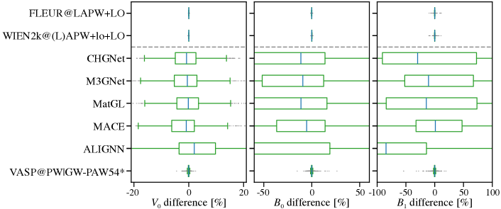
Figure 1: Boxplot showing the relative error in $V_{0}$, $B_{0}$ and $B_{1}$ for the different uMLIPs analyzed in this work and some of the ab initio codes considered in Ref. ³⁸ with respect to the average of the AE reference results.

As a first test, we use the protocol for the equation of state (EOS) detailed in Ref. ³⁸, where a high-quality reference dataset of EOS for 960 cubic crystal structures is generated by employing two all-electron (AE) codes. This dataset includes all elements from Z = 1 (hydrogen) to Z = 96 (curium). For each element, four mono-elemental cubic crystals (unaries structures) are considered, in the face-centered cubic (FCC), body-centered cubic (BCC), simple cubic (SC), and diamond crystal structure, respectively. Besides, six cubic oxides (oxides structures) are included for each element X, with chemical formula X₂O, XO, X₂O₃, XO₂, X₂O₅, and XO₃, respectively. While in Ref. ³⁸ this dataset is used to gauge the precision and transferability of nine pseudopotential-based ab initio codes, we use it here to assess the five tested uMLIPs.

In Fig. 1 the relative errors on the uMLIPs predictions for the equilibrium volume $V_{0}$, the bulk modulus $B_{0}$, and its derivative with respect to the pressure $B_{1}$ obtained based on a fit ³⁸ of the EOS, are compared with the analogous errors from selected ab initio methods employed in Ref. ³⁸. FLEUR ⁴⁵ and WIEN2K ⁴⁶ are AE codes while VASP implements the projector augmented-wave method (PAW) method ⁴⁷ with a planewave basis set. The errors reported in Fig. 1 are calculated respect to the average of the AE methods considered here, i.e., FLEUR ⁴⁵ and WIEN2K ⁴⁶.

Also, as in Ref. ³⁸, the EOS computed with two different computational approaches $a$ and $b$ ($E_{a}(V)$ and $E_{b}(V)$) are compared through two metrics $\epsilon(a,b)$ and $\nu(a,b)$. The first is a renormalized dimensionless version of the metrics $\Delta(a,b)$ introduced in Ref. ⁴⁸:

$$\epsilon(a,b)=\sqrt{\frac{\sum_{i}\left[E_{a}(V_{i})-E_{b}(V_{i})\right]^{2}}{\sqrt{\sum_{i}\left[E_{a}(V_{i})-\left<E_{a}\right>\right]^{2}\sum_{i}\left[E_{b}(V_{i})-\left<E_{b}\right>\right]^{2}}}},$$ (1)

where the index $i$ runs over the explicit calculations of $E_{a,b}(V)$ for the different methods and $\left<E_{a,b}\right>$ is the integral average of $E_{a,b}(V)$ over the considered volume range. The second metric depends directly on the physically measurable quantities $V_{0}$, $B_{0}$, and $B_{1}$. It captures the relative deviation for each of these three parameters between the two computational approaches $a$ and $b$:

$$\nu_{w_{V_{0}},w_{B_{0}},w_{B_{1}}}(a,b)=100\sqrt{\sum_{Y=V_{0},B_{0},B_{1}}\left[w_{Y}\frac{Y_{a}-Y_{b}}{(Y_{a}-Y_{b})/2}\right]^{2}},$$ (2)

where $w_{V_{0}}$, $w_{B_{0}}$, and $w_{B_{1}}$ are appropriately chosen weights (see Ref. ³⁸). Here, $a$ and $b$ are a uMLIP and the average of the AE methods considered here, i.e., FLEUR ⁴⁵ and WIEN2K ⁴⁶, respectively. Heatmaps of the periodic table with the values of the comparison metrics $\varepsilon$ and $\nu$ obtained with all the different uMLIPs are reported in Fig. 2 in the Supplemental Material.

It should be noted that most structures in the dataset used in this EOS test are not stable in nature. Therefore, it is very likely that these configurations were not included in the dataset used to train the uMLIPs. As a consequence, it is not surprising that the uMLIPs are not able to predict the correct energy versus volume curve for a significant fraction of systems (Figs. 1-5 in the Supplementary Material). Nevertheless, even for those systems for which a physical EOS is obtained, the precision and transferability is still far from the one that can be achieved with state–of-the-art pseudopotential-based ab initio techniques, as can be observed in Fig. 1. This is a very stringent test for uMLIPs, especially given the effort made in Ref. ³⁸ to improve the precision and the transferability of pre-existent pseudopotential tables used for ab initio calculations. Yet these results suggest that uMLIPs predictions should be taken with some caution and, if possible, validated a posteriori via ab initio calculations, especially if the chemical/physical environment under study is not properly included in the training dataset. The precision of uMLIPs can be improved after retraining the model by including additional ab initio data capturing the chemical/physical configurations under investigation. However, despite their relevance, these topics are beyond the scope of the present work and are left for future investigation.

2.2 Atomic and lattice relaxations

To test the accuracy of the different uMLIPs further, we prepare a dataset with 19998 materials consisting of unary and binary (with 6903 element combinations) phases in MP. It is worthwhile to highlight that the MP database contains structures relaxed with VASP ⁴⁴ with the PBE functional. The distribution of the chosen dataset among the chemical elements is reported in Fig. 2. We use the different uMLIPs to perform energy calculations both with no structural optimization (we call these “one-shot” calculations) and with structural optimization. The latter are of two types: (i) only the atomic positions are relaxed (we call these “ion-relax” calculations), and (ii) both atomic positions and cell parameters (i.e., lattice parameters and angles) are relaxed (we call these “cell-relax” calculations). For the structural optimizations, in some cases the calculation stops due to errors while building the graph representation (e.g., given that isolated atoms are found in the structure). Calculations for which this problem appears are tagged as problematic. In another non-negligible number of cases, that we tag as unconverged, the relaxation algorithm is not able to reach the stopping criterion before 150 steps. Finally, we tag as converged the calculations where the stopping criterion is met in less than 150 steps. Additional details on the relaxation algorithm are given in Sec. 4.

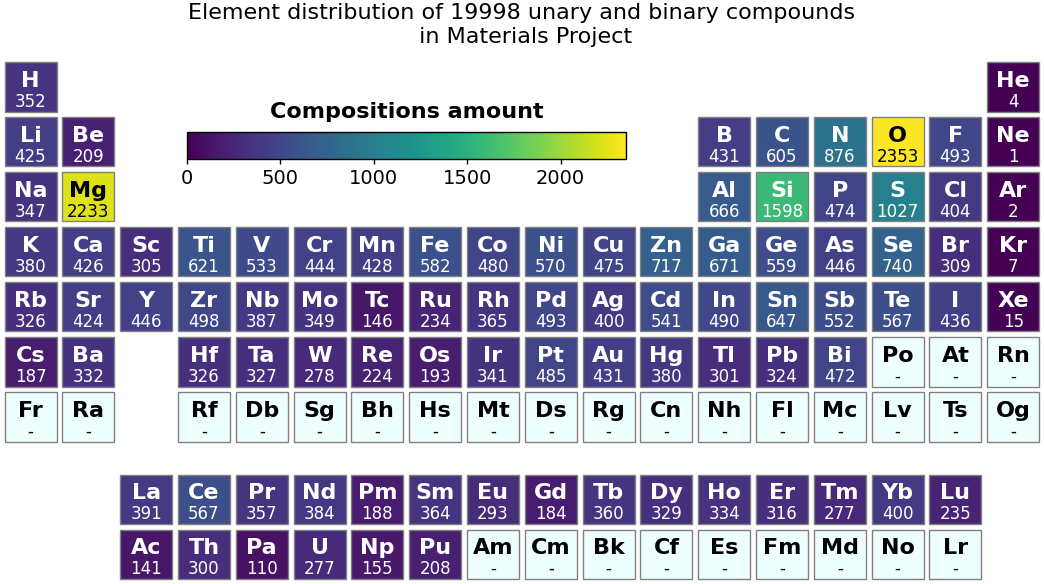
Figure 2: Heatmaps of the periodic table for the dataset chosen for the structural relaxations (unaries and binaries), expressing the data distribution over the chemical composition space. The figure has been produced with the pymatviz tool ⁴⁹.

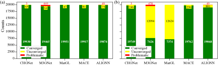
Figure 3: Analysis of the convergence of the different uMLIPs for geometry optimization. In panel (a), only the atomic positions are relaxed, while the cell parameters are kept fixed at the original values. In panel (b), both the atomic positions and the cell parameters are relaxed. As explained in the text, a calculation is considered to be converged when the relaxation criteria (in terms of forces and stresses) are met within 150 steps.

In Fig 3, we report the number of occurrences of the problematic, unconverged, and converged tags from the different uMLIPs for the two types of structural optimization. When only the atomic positions are relaxed (Fig 3(a)), the fraction of problematic or unconverged cases is very limited. The best performance is achieved by MatGL (with only 0.2% of unconverged cases), while the worst case is M3GNet (with 2.4% of problematic cases). The fraction of unconverged calculations increases significantly (from 3 to more than 200 times across the uMLIPs) when both atomic positions and cell parameters are optimized (Fig 3(b)). M3GNet and MatGL (both about 60% of unconverged cases) are the most critical cases. The high percentage of unconverged calculations from these two uMLIPs is probably related to the large values of the stress tensors along the structural optimization, which prevent the cell to relax. Full relaxation with CHGNet, MACE, and ALIGNN lead to significantly lower fractions of unconverged results (1.2%, 1.2%, and 4.4%, respectively), with CHGNet and MACE performing very robustly. In the following, we discuss only results from the converged geometry optimizations.

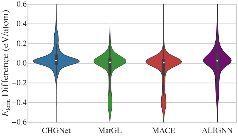
Figure 4: Violin plots showing the distribution of $\Delta E_{\textrm{form}}$ (Eq. (4) from one-shot calculations for the different uMLIPs.

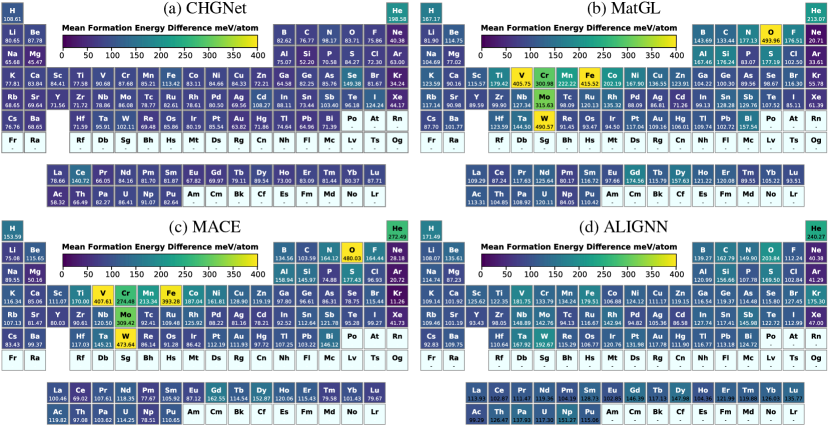
Figure 5: Heatmaps of the periodic table for the absolute values of $\Delta E_{\textrm{form}}$ for the one-shot calculations from the different uMLIPS: (a) CHGNet, (b) MatGL, (c) MACE, and (d) ALIGNN. The figure has been produced with the pymatviz tool ⁴⁹.

To compare the predictive performance of these uMLIPs regarding energy levels, we also used a benchmark based on the formation energy, defined as

$$E_{\textrm{form}}[A_{a}B_{b}]=E[A_{a}B_{b}]-x_{a}E[A]-x_{b}E[B],$$ (3)

where $E[A_{a}B_{b}]$ is the total energy for the phase of interest, $a$ and $b$ reflect the composition of the compound with their respective fractions $x_{a}=a/(a+b)$ and $x_{b}=b/(a+b)$, and $E[A]$ and $E[B]$ the lowest possible energies of the elemental compounds $A$ and $B$, respectively. The ability of the uMLIPs in predicting formation energies is evaluated again as a difference from the MP values, i.e.,

$$\Delta E_{\textrm{form}}=E_{\textrm{form}}^{\text{MP}}-E_{\textrm{form}}^{\text{uMLIP}},$$ (4)

with $E_{\textrm{form}}^{\text{MP}}$ and $E_{\textrm{form}}^{\text{uMLIP}}$ being the formation energy from Eq. (3) calculated with MP and the uMLIP model, respectively. M3GNet had to be excluded due to the problematic calculations. Indeed, we could not obtain any energy for a number of elemental compounds (e.g., K, and Rb). Therefore, the number of available formation energies would have been significantly lower for M3GNET than for other uMLIPs. For the same reason (i.e., maximizing the number of formation energies in our dataset), we chose to work with the one-shot results.

In Fig. 4 we report the distribution of $\Delta E_{\textrm{form}}$ (Eq.(4)) for the one-shot calculations using the different uMLIPs. Figure 5 shows the distribution of the absolute mean values of $\Delta E_{\textrm{form}}$ on the chemical space for the different uMLIPs, i.e., the average of the absolute value of $\Delta E_{\textrm{form}}$ over all the chemical systems containing a given element. CHGNet has the best performance for chemical systems containing the transition metals V, Cr, and W, which is likely due to the inclusion of the magnetic moments in this model. MatGL and MACE are less performant for O, V, Fe, and W, where CHGNet and ALIGNN perform very well instead. Besides, MatGL and MACE have slightly poorer performance with respect to CHGNet for chemical compositions including halogens. The performance of the different uMLIPs for $\Delta E_{\textrm{form}}$ (Eq. (4)) for the one-shot calculations is reported in Table 1. CHGNet shows better performance than the other uMLIPs, with the smallest MAE and RMSE and the highest R², which is 0.081, 0.158 and 0.974, respectively. In turn, CHGNet outperforms the other uMLIPs in the one-shot calculations (Fig. 4 and Table 1), while having almost the same number of converged results (i.e., successful structural optimizations) as MACE, and as double as the number of converged results as MatGL (Fig. 3).

In Fig.6 and Table 2 we summarize the ability of the different uMLIPs (cell-relax calculations) to predict cell parameters, i.e., lattice parameters, angles, and volume. As done for the formation energies (Fig. 4, Eq. (4), and Table 1), we compare the uMLIPs results with the MP values, e.g., for the volume we consider

$$\Delta_{\textrm{rel}}V=1-\frac{V^{\mathrm{uMLIP}}}{V^{\mathrm{MP}}},$$ (5)

where $V^{\mathrm{MP}}$ and $V^{\mathrm{uMLIP}}$ are the cell volume from MP and from the uMLIP model (cell-relax calculations), respectively. In Fig.6 we report the distribution of $\Delta_{\textrm{rel}}V$. CHGNet and ALIGNN outperform the other uMLIPs, with a narrower distribution of $\Delta_{\textrm{rel}}V$. M3GNet is the worst performing, while MatGL and MACE have a somehow intermediate performance. In Table 2, we also report the Mean Absolute Relative Error (MARE) on the predicted lattice parameters (lengths and angles). We observe that CHGNet and MACE show similar performance. In fact, the violin plots are strongly influenced by the presence of outliers. ALIGNN also has a very good performance, while M3GNet and MatGL present significant MARE values (not to mention that they also lead to the highest numbers of unconverged cases).

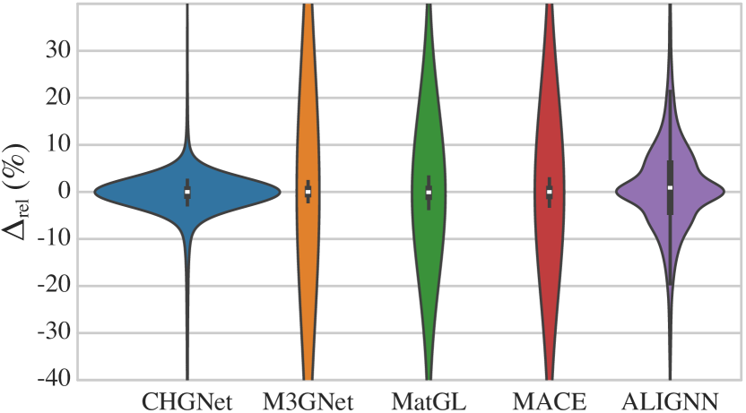
Figure 6: Violin plots of the relative difference between the cell volume from MP and from the different uMLIPs predictions (Eq. (5)). Only converged runs are included in the plot.

uMLIP	MAE	RMSE	R2
CHGNet	0.081	0.158	0.974
MatGL	0.158	0.319	0.892
MACE	0.148	0.308	0.900
ALIGNN	0.129	0.249	0.939

Table 1: Performance of the uMLIPs in predicting the formation energy for one-shot calculations.

uMLIP	a	b	c	$\alpha$	$\beta$	$\gamma$
CHGNet	2.3	2.3	2.7	0.9	0.7	1.3
M3GNet	33.4	33.3	33.5	14.3	14.2	14.1
MatGL	34.0	33.5	34.3	14.5	14.4	14.4
MACE	3.0	3.2	3.3	0.9	0.7	1.3
ALIGNN	6.9	6.5	7.1	1.8	1.7	2.1

Table 2: Mean Absolute Relative Error (MARE in %) of the different uMLIPs in predicting the lattice lengths and angles.

2.3 Vibrational properties

In this section, we analyze the capability of uMLIPs to reproduce the vibrational properties of crystalline materials using accurate ab initio results reported in a previous work ³⁹ as a reference. From the structures in Ref. ³⁹ we select those whose energy above hull is zero both in the MP database and from the uMLIP calculations (cell-relax), leading to 101 structures. Phonons are computed using the finite displacement method as implemented in the phonopy package ^{50, 51}. Further details on the protocol employed to compute phonons with uMLIPs are provided in Section 4. By exploiting the finite displacement method to compute phonons, this study indirectly probes the quality of the uMLIPs-calculated forces when atoms are slightly displaced away from the equilibrium positions. From a methodological point of view we note that, already when ab initio engines are used, the accuracy of phonon calculations from the finite displacement method is rather sensitive to the quality of the force calculations in the supercell. Since by construction these forces are less accurate when calculated from uMLIP models than from ab initio methods, it is reasonable to expect some non-negligible discrepancy between uMLIPs and ab initio phonon calculations. Also, as discussed in more detail in Sec. 4, the MLIP architectures at the basis of the universal models considered in this study cannot predict the long-range dipolar contributions to the interatomic force constants of polar materials ^{52, 53}. In order to obtain a reliable Fourier phonon interpolation in the case of polar materials, the uMLIP-calculated forces should therefore be augmented with the ML electronic dielectric tensor and the Born effective charges which are not available at present (see Sec. 4 for further details).

For these reasons, when comparing uMLIPs results with ab initio data, we choose a rather generous metrics, i.e., the MAE between the uMLIPs and the ab initio phonon band structures computed along a high-symmetry $\mathbf{q}$-path ⁵⁴:

$$\text{MAE}=\dfrac{1}{N_{\mathbf{q}}}\sum_{\mathbf{q}\nu}|{\omega_{{{\mathbf{q}\nu}}}}^{\text{uMLIP}}-{\omega_{{{\mathbf{q}\nu}}}}^{\text{DFPT}}|.$$ (6)

In Eq. (6), $\omega_{\mathbf{q}\nu}$ is the phonon energy in meV, $\nu$ is the branch index, $N_{\mathbf{q}}$ is the number of wavevectors used to sample the $\mathbf{q}$-path, and $\omega_{\mathbf{q}\nu}^{\text{uMLIP}}$, $\omega_{\mathbf{q}\nu}^{\text{DFPT}}$ are the phonon energies computed using the uMLIP model and density-functional perturbation theory (DFPT) with ABINIT ³⁹, respectively. Table 3 reports the minimum, maximum and average values of the MAE in the phonon band structures obtained from the different uMLIPs (Eq. (6), while the MAE distribution in terms of violin plots is given in panel (a) of Fig. 7.

uMLIP	MIN_MAE	MAX_MAE	MEAN_MAE
CHGNet	0.818	16.318	7.711
M3GNet	2.033	15.848	6.925
MatGL	2.678	26.299	7.696
MACE	0.312	5.573	3.682
ALIGNN	11.792	49.335	30.018

Table 3: Minimum, maximum and average MAE in meV for the phonon band structures computed from different uMLIPs.

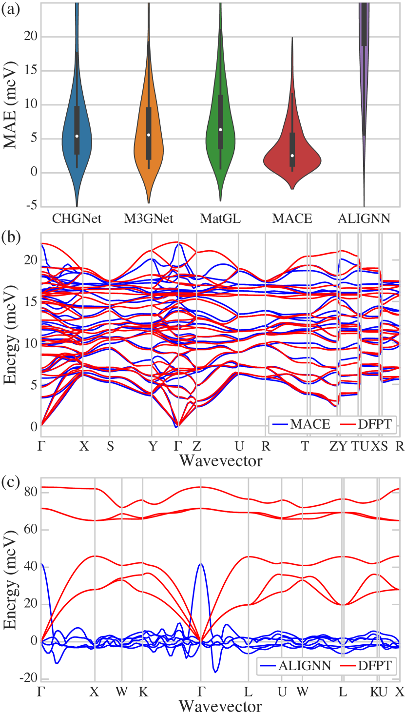
Figure 7: (a) Violins plots of the MAE (Eq. (6)) on the computed phonon band structures from uMLIPs and DFPT. (b) Comparison of the phonon band structures computed with DFPT and MACE for the compound (mp-567744: SrBr₂) with the smallest MAE (0.3 meV). (c) Comparison of the phonon band structures computed with DFPT and ALIGNN for the compound (mp-422: BeS) with the largest MAE (49.3 meV).

However, from panel (a) of Fig. 7 and Table  3, as anticipated above, we observe a non-ideal agreement between uMLIPs-calculated and ab initio-calculated vibrational properties. In addition to the fundamental reasons discussed already, a source of discrepancy could come, in this particular study, from the fact that the PBEsol exchange-correlation functional was used in Ref. ³⁹ while the uMLIPs have been trained using PBE data with the inclusion of U-corrections for certain systems (the only exception being ALIGNN that was trained on optB88vdW data). In panel (b) of Fig. 7 we report the phonon band structure for the system with the lowest MAE (0.312 meV, obtained from MACE, Table 3), which is Sr₄Br₈ (mp-567744). Conversely, in panel (c) of Fig. 7 we report the phonon band structure for the system with the highest MAE (49.335 meV, obtained from ALIGNN, Table 3), which is BeS (mp-422). For the latter, the uMLIP predicts vibrational instabilities that are not observed in the ab initio results.

To summarize, our results indicate that presently available uMLIPs can predict ab initio vibrational properties with a typical error of 3.682 meV in the best case scenario. This value should be considered as a lower bound as the discrepancy is expected to increase significantly if the electronic dielectric tensor and the Born effective charges cannot be predicted with ML techniques.

In the opinion of the authors, the predictive behavior of uMLIPs for vibrational properties can be improved by training new uMLIPs with larger weights for the forces loss function but it is also clear that for accurate ML-based predictions in polar materials, one needs uMLIPs capable of inferring the long-range part of the dynamical matrix. All this being said, we believe that uMLIPs represent an efficient and promising approach to perform an initial screening for vibrational and thermodynamic properties, especially in a high-throughput context in which high accuracy is not necessarily needed.

3 Conclusions

We present a systematic assessment of various universal machine-learning interatomic potentials (uMLIPs) by investigating their capability to reproduce ab initio results for several important physical properties such as equation of states, relaxed geometries, formation energies and vibrational properties. Among the considered uMLIPs, we find that CHGNet outperforms the others, showing superior precision in predicting the relaxed geometry and formation energy, also considering the number of converged results. CHGNet also has some advantages when considering systems containing elements such as O and some of the transition metal elements. MACE, on the other hand, excels when predicting vibrational properties and, at the same time, is able to infer all the other physical properties with good precision. For what concerns ALIGNN, despite trained with different dataset, it still shows excellent results when predicting lattice parameters and formation energies. M3GNet and MatGL reveal to be the most problematic ones when performing geometry optimization at variable cell. This underscores the need for further optimization and training to fully exploit the capability of ML techniques across a broader range of applications. The choice of a particular uMLIP for specific applications should take into account an appropriate balance between accuracy and computational efficiency. Future work should aim at enhancing the performance of these potentials further, particularly focusing on areas where current uMLIPs exhibit limitations such as more accurate prediction of forces and stresses or the capability of learning Born effective charges and electronic dielectric tensors that are crucial for the vibrational properties of polar materials. Our work will hopefully pave the way towards a more systematic assessment of uMLIPs in different scenarios and the establishment of a standardized benchmark set that can be used to gauge the precision and transferability of uMLIPs.

4 Methods

The calculations are performed with the AbiPy package ^{40, 41}, more specifically the abiml.py script that provides a unified interface that allows one to perform different types of calculations such as structural relaxations, molecular dynamics or NEB using the algorithms implemented in ASE ⁵⁵ and different uMLIPs as calculators. The following versions are used to produce the results reported in this work: Python 3.11, Pymatgen 2023.7.17, AbiPy 0.9.6, Abinit 9.8.4, M3GNet:0.2.4, CHGNet:0.3.2, ALIGNN: 2023.10.1, MatGL: 0.9.1, MACE: mace_mp_0 with mace-torch 0.3.4, and ASE: 3.22.1.

Structural relaxations are performed using the ASE optimizer, employing the BFGS algorithm. To ensure good trade-off between accuracy and computational cost, the stopping criterion fmax is set to 0.1 eV/Å. If the stopping criterion is not met at a maximum number of iterations set to 150, the calculation is considered unconverged. This is justified by the fact that all the initial structures in our dataset are taken from the Materials Project ¹⁹, where they have been already relaxed with VASP with the PBE functional, and are supposed to be included in the set used to train the uMLIPs (with the exception of ALIGNN).

For the phonon calculations, we first perform a structural relaxation with the uMLIPs from the crystalline structures employed in ³⁹. Only the atomic positions are relaxed at fixed cell in order to avoid spurious effects due to the change of the lattice parameters with respect to the reference DFT results. The relaxed configuration is then used to compute vibrational properties using the finite displacement method implemented in phonopy ^{50, 51} with a displacement of 0.01 Å. In each calculation, the real-space supercell is matched with the $\mathbf{q}$-mesh employed in ³⁹ to compute the dynamical matrix with the DFPT part of Abinit ^{40, 41}. It is noteworthy that the uMLIPs employed in this work lack the capability to predict the electronic dielectric tensor $\epsilon^{\infty}$ and the Born effective charge tensor ${\bf Z}^{*}_{\kappa}$ where $\kappa$ is the index of the atom in the unit cell. As discussed in ^{52, 53}, these quantities are needed to model the long-range dipolar contribution to the interatomic force constants in polar materials. This term is indeed responsible for the LO-TO splitting as well as for the non-analytical behaviour of the vibrational spectrum near $\textbf{q}=0$. Its correct numerical treatment is therefore crucial to obtain an accurate Fourier interpolation of the dynamical matrix at arbitrary $\mathbf{q}$-points. For this reason, in all phonopy calculations we use the ab initio values of $\epsilon^{\infty}$ and ${\bf Z}^{*}_{\kappa}$ obtained with Abinit to model long-range interactions. The ab initio phonon dispersions is obtained by using the anaddb post-processing tool using the DDB files retrieved from the MP database to compare the different phonon dispersions between uMLIPs and ab initio DFPT results.
Figure 1 and the heatmaps of the periodic table in the Supplemental Material have been produced using the ab initio results and the open source python scripts available in the acwf-verification-scripts github repository.

*Author contributions

G.-M. R. designed the research topic and coordinated the whole project. All authors provided the ideas underlying this work, contributed to its development, and discussed the findings reported in the paper. All authors took part to the writing and reviewing of the paper, and to the final approval of its completed version. H. Y. and M. G. executed the calculations presented. M. G. developed and maintained the software infrastructure.

*Acknowledgments

Computational resources have been provided by the supercomputing facilities of the Université catholique de Louvain (CISM/UCL), and the Consortium des Equipements de Calcul Intensif en Fédération Wallonie Bruxelles (CECI).

*Financial disclosure

None reported.

Conflict of interest

The authors declare no potential conflict of interests.

*Supporting information

Additional supporting information may be found in the online version of the article at the publisher’s website.

References

- 1 Frenkel D, Smit B. Understanding molecular simulation: from algorithms to applications. Elsevier, 2023.
- 2 Hohenberg P, Kohn W. Inhomogeneous Electron Gas. Phys. Rev.. 1964;136(3B):B864-B871. doi: 10.1103/physrev.136.b864
- 3 Kohn W, Sham LJ. Self-Consistent Equations Including Exchange and Correlation Effects. Phys. Rev.. 1965;140(4A):A1133-A1138. doi: 10.1103/physrev.140.a1133
- 4 Payne MC, Teter MP, Allan DC, Arias T, Joannopoulos aJ. Iterative minimization techniques for ab initio total-energy calculations: molecular dynamics and conjugate gradients. Reviews of modern physics. 1992;64(4):1045.
- 5 Marzari N, Ferretti A, Wolverton C. Electronic-structure methods for materials design. Nature Materials. 2021;20(6):736–749. doi: 10.1038/s41563-021-01013-3
- 6 Goddard I. Classical Force Fields and Methods of Molecular Dynamics:1063–1072; Springer International Publishing . 2021.
- 7 Zuo Y, Chen C, Li X, et al. Performance and cost assessment of machine learning interatomic potentials. The Journal of Physical Chemistry A. 2020;124(4):731–745.
- 8 Deringer VL, Caro MA, Csányi G. Machine Learning Interatomic Potentials as Emerging Tools for Materials Science. Advanced Materials. 2019;31(46). doi: 10.1002/adma.201902765
- 9 Behler J, Parrinello M. Generalized Neural-Network Representation of High-Dimensional Potential-Energy Surfaces. Physical Review Letters. 2007;98(14). doi: 10.1103/physrevlett.98.146401
- 10 Bartók AP, Payne MC, Kondor R, Csányi G. Gaussian Approximation Potentials: The Accuracy of Quantum Mechanics, without the Electrons. Physical Review Letters. 2010;104(13). doi: 10.1103/physrevlett.104.136403
- 11 Thompson A, Swiler L, Trott C, Foiles S, Tucker G. Spectral neighbor analysis method for automated generation of quantum-accurate interatomic potentials. Journal of Computational Physics. 2015;285:316–330. doi: 10.1016/j.jcp.2014.12.018
- 12 Schütt KT, Sauceda HE, Kindermans PJ, Tkatchenko A, Müller KR. SchNet – A deep learning architecture for molecules and materials. The Journal of Chemical Physics. 2018;148(24). doi: 10.1063/1.5019779
- 13 Drautz R. Atomic cluster expansion for accurate and transferable interatomic potentials. Physical Review B. 2019;99(1). doi: 10.1103/physrevb.99.014104
- 14 Lilienfeld vOA, Burke K. Retrospective on a decade of machine learning for chemical discovery. Nature Communications. 2020;11(1). doi: 10.1038/s41467-020-18556-9
- 15 Batzner S, Musaelian A, Sun L, et al. E(3)-equivariant graph neural networks for data-efficient and accurate interatomic potentials. Nature Communications. 2022;13(1). doi: 10.1038/s41467-022-29939-5
- 16 Ko TW, Ong SP. Recent advances and outstanding challenges for machine learning interatomic potentials. Nature Computational Science. 2023;3(12):998–1000. doi: 10.1038/s43588-023-00561-9
- 17 Deringer VL, Bartók AP, Bernstein N, Wilkins DM, Ceriotti M, Csányi G. Gaussian Process Regression for Materials and Molecules. Chemical Reviews. 2021;121(16):10073–10141. doi: 10.1021/acs.chemrev.1c00022
- 18 Chen C, Ye W, Zuo Y, Zheng C, Ong SP. Graph Networks as a Universal Machine Learning Framework for Molecules and Crystals. Chemistry of Materials. 2019;31(9):3564–3572. doi: 10.1021/acs.chemmater.9b01294
- 19 Jain A, Ong SP, Hautier G, et al. Commentary: The Materials Project: A materials genome approach to accelerating materials innovation. APL Materials. 2013;1(1). doi: 10.1063/1.4812323
- 20 Perdew JP, Burke K, Ernzerhof M. Generalized Gradient Approximation Made Simple. Physical Review Letters. 1996;77(18):3865–3868. doi: 10.1103/physrevlett.77.3865
- 21 Chen C, Ong SP. A universal graph deep learning interatomic potential for the periodic table. Nature Computational Science. 2022;2(11):718–728. doi: 10.1038/s43588-022-00349-3
- 22 Deng B, Zhong P, Jun K, et al. CHGNet as a pretrained universal neural network potential for charge-informed atomistic modelling. Nature Machine Intelligence. 2023;5(9):1031–1041. doi: 10.1038/s42256-023-00716-3
- 23 https://github.com/materialsvirtuallab/matgl; . Accessed: 2024-02-29.
- 24 Choudhary K, DeCost B, Major L, Butler K, Thiyagalingam J, Tavazza F. Unified graph neural network force-field for the periodic table: solid state applications. Digital Discovery. 2023;2(2):346–355. doi: 10.1039/d2dd00096b
- 25 Choudhary K, Garrity KF, Reid ACE, et al. The joint automated repository for various integrated simulations (JARVIS) for data-driven materials design. npj Computational Materials. 2020;6(1). doi: 10.1038/s41524-020-00440-1
- 26 Klimeš J, Bowler DR, Michaelides A. Chemical accuracy for the van der Waals density functional. Journal of Physics: Condensed Matter. 2009;22(2):022201. doi: 10.1088/0953-8984/22/2/022201
- 27 Batatia I, Benner P, Chiang Y, et al. A foundation model for atomistic materials chemistry. arXiv preprint arXiv:2401.00096. 2023.
- 28 Batatia I, Kovacs DP, Simm G, Ortner C, Csanyi G. MACE: Higher Order Equivariant Message Passing Neural Networks for Fast and Accurate Force Fields. In: Koyejo S, Mohamed S, Agarwal A, Belgrave D, Cho K, Oh A. , eds. Advances in Neural Information Processing Systems 35 (NeurIPS 2022). 35. NeurIPS. Curran Associates, Inc. 2022:11423–11436.
- 29 Merchant A, Batzner S, Schoenholz SS, Aykol M, Cheon G, Cubuk ED. Scaling deep learning for materials discovery. Nature. 2023;624(7990):80–85. doi: 10.1038/s41586-023-06735-9
- 30 Takamoto S, Shinagawa C, Motoki D, et al. Towards universal neural network potential for material discovery applicable to arbitrary combination of 45 elements. Nature Communications. 2022;13(1). doi: 10.1038/s41467-022-30687-9
- 31 Takamoto S, Okanohara D, Li QJ, Li J. Towards universal neural network interatomic potential. Journal of Materiomics. 2023;9(3):447–454. doi: 10.1016/j.jmat.2022.12.007
- 32 Takamoto S, Izumi S, Li J. TeaNet: Universal neural network interatomic potential inspired by iterative electronic relaxations. Computational Materials Science. 2022;207:111280. doi: 10.1016/j.commatsci.2022.111280
- 33 Smith JS, Isayev O, Roitberg AE. ANI-1: an extensible neural network potential with DFT accuracy at force field computational cost. Chemical Science. 2017;8(4):3192–3203. doi: 10.1039/c6sc05720a
- 34 Smith JS, Nebgen BT, Zubatyuk R, et al. Approaching coupled cluster accuracy with a general-purpose neural network potential through transfer learning. Nature Communications. 2019;10(1). doi: 10.1038/s41467-019-10827-4
- 35 Zubatyuk R, Smith JS, Leszczynski J, Isayev O. Accurate and transferable multitask prediction of chemical properties with an atoms-in-molecules neural network. Science Advances. 2019;5(8). doi: 10.1126/sciadv.aav6490
- 36 Lopanitsyna N, Fraux G, Springer MA, De S, Ceriotti M. Modeling high-entropy transition metal alloys with alchemical compression. Physical Review Materials. 2023;7(4). doi: 10.1103/physrevmaterials.7.045802
- 37 Choudhary K, DeCost B. Atomistic Line Graph Neural Network for improved materials property predictions. npj Computational Materials. 2021;7(1). doi: 10.1038/s41524-021-00650-1
- 38 Bosoni E, Beal L, Bercx M, et al. How to verify the precision of density-functional-theory implementations via reproducible and universal workflows. Nature Reviews Physics. 2023;6(1):45–58. doi: 10.1038/s42254-023-00655-3
- 39 Petretto G, Dwaraknath S, P.C. Miranda H, et al. High-throughput density-functional perturbation theory phonons for inorganic materials. Sci. Data. 2018;5:180065. doi: 10.1038/sdata.2018.65
- 40 Gonze X, Amadon B, Antonius G, et al. The Abinit project: Impact, environment and recent developments. Computer Physics Communications. 2020;248:107042. doi: 10.1016/j.cpc.2019.107042
- 41 Romero AH, Allan DC, Amadon B, et al. ABINIT: Overview and focus on selected capabilities. The Journal of Chemical Physics. 2020;152(12). doi: 10.1063/1.5144261
- 42 Hamann DR. Optimized norm-conserving Vanderbilt pseudopotentials. Phys. Rev. B. 2013;88(8):085117. doi: 10.1103/physrevb.88.085117
- 43 Setten vM, Giantomassi M, Bousquet E, et al. The PseudoDojo: Training and grading a 85 element optimized norm-conserving pseudopotential table. Comput. Phys. Commun.. 2018;226:39-54. doi: 10.1016/j.cpc.2018.01.012
- 44 Kresse G, Joubert D. From ultrasoft pseudopotentials to the projector augmented-wave method. Phys. Rev. B. 1999;59:1758–1775. doi: 10.1103/PhysRevB.59.1758
- 45 Wortmann, Daniel and Michalicek, Gregor and Hilgers, Robin and Neukirchen, Alexander and Janssen, Henning and Grytsiuk, Uliana and Broeder, Jens and Gerhorst, Christian-Roman . FLEUR. Web Page;
- 46 Blaha P, Schwarz K, Tran F, Laskowski R, Madsen GKH, Marks LD. WIEN2k: An APW+lo program for calculating the properties of solids. The Journal of Chemical Physics. 2020;152(7):074101. doi: 10.1063/1.5143061
- 47 Blöchl PE. Projector augmented-wave method. Phys. Rev. B. 1994;50:17953–17979. doi: 10.1103/PhysRevB.50.17953
- 48 Lejaeghere K, Bihlmayer G, Björkman T, et al. Reproducibility in density functional theory calculations of solids. Science. 2016;351(6280):aad3000.
- 49 Riebesell J. Pymatviz: visualization toolkit for materials informatics. Web Page; 2022. 10.5281/zenodo.7486816 - https://github.com/janosh/pymatviz
- 50 Togo A, Chaput L, Tadano T, Tanaka I. Implementation strategies in phonopy and phono3py. J. Phys. Condens. Matter. 2023;35(35):353001. doi: 10.1088/1361-648X/acd831
- 51 Togo A. First-principles Phonon Calculations with Phonopy and Phono3py. J. Phys. Soc. Jpn.. 2023;92(1):012001. doi: 10.7566/JPSJ.92.012001
- 52 Gonze X, Lee C. Dynamical matrices, Born effective charges, dielectric permittivity tensors, and interatomic force constants from density-functional perturbation theory. Phys. Rev. B. 1997;55(16):10355-10368. doi: 10.1103/physrevb.55.10355
- 53 Baroni S, Gironcoli dS, Dal Corso A, Giannozzi P. Phonons and related crystal properties from density-functional perturbation theory. Rev. Mod. Phys.. 2001;73(2):515-562. doi: 10.1103/revmodphys.73.515
- 54 Setyawan W, Curtarolo S. High-throughput electronic band structure calculations: Challenges and tools. Computational Materials Science. 2010;49(2):299–312. doi: 10.1016/j.commatsci.2010.05.010
- 55 Hjorth Larsen A, Jørgen Mortensen J, Blomqvist J, et al. The atomic simulation environment—a Python library for working with atoms. Journal of Physics: Condensed Matter. 2017;29(27):273002. doi: 10.1088/1361-648x/aa680e