Propagation speeds of relativistic conformal fluids from a generalized relaxation time approximation

Abstract

We compute the propagation speeds for a conformal real relativistic fluid. We begin from a kinetic equation in the relaxation time approximation, where the relaxation time is an arbitrary function of the particle energy in the Landau frame. We propose a parameterization of the one particle distribution function designed to contain a second order Chapman-Enskog solution as a particular case. We derive the hydrodynamic equations applying the moments method to this parameterized one particle distribution function, and solve for the propagation speeds of linearized scalar, vector and tensor perturbations. For relaxation times of the form $\tau=\tau_{0}(-\beta_{\mu}p^{\mu})^{-a}$, with $-\infty<a<2$, where $\beta_{\mu}=u_{\mu}/T$ is the temperature vector in the Landau frame, we show that the Anderson-Witting prescription $a=1$ yields the fastest speeds.

I Introduction

The success of hydrodynamics in the description of the early stages of relativistic heavy ion collisions [1, 2] and the promise of relevant cosmological applications [3, 4, 5] have turned relativistic real fluids into an active area of research [6, 7]. However, no single set of hydrodynamic equations has been universally accepted as the proper description of these systems. In particular, attempts to derive hydrodynamics purely from macroscopic considerations [8, 9, 10, 11] have proven not compelling enough. For this reasons, the usual path to hydrodynamics is to derive it from a more microscopic theory, usually kinetic [12, 13, 14, 15] or field theory [16, 17]. In this paper, we shall adopt kinetic theory as the fundamental description, and derive hydrodynamic equations from it.

Given the complexity of nonlinear collision operators such as Boltzmann’s, oftentimes it is preferred to work under the Relaxation Time Approximation (RTA), which assumes a linear kinetic equation parametrized by a relaxation time. An early implementation of the RTA is Marle’s [18, 19], which assumes a single, momentum independent relaxation time. This was later improved on by Anderson and Witting [20, 21], which assumed the relaxation time was inversely proportional to the energy of the particle in the Landau frame of the fluid. However successful, both Marle and Anderson-Witting RTA’s severely distort the structure of the linearized Boltzmann equation, and their validity is doubtful for soft collision terms, where the continuous spectrum of the linearized collision operator reaches up to the zero eigenvalue associated with the hydrodynamic modes.

This has led to more general implementations of the RTA [22, 23] where different modes were allowed to relax at different rates. However, simply allowing the relaxation times to be a function of energy other than constant or linear is not satisfactory as it may violate energy-momentum conservation. Rather the RTA must be implemented preserving the Hilbert space structure of the space of linearized one-particle distribution function (1-pdf’s). A kinetic equation allowing for an momentum dependent relaxation time consistent with energy-momentum conservation was introduced in [24, 25]. In this paper we shall elaborate on this proposal. In particular, we shall show how to produce a RTA matching any prescribed spectrum for the linearized collision operator, either soft or hard. Not been able to do this is one of the main drawbacks of the usual formulations of the RTA. See also [26, 27, 28, 29, 30, 31, 32, 33, 34, 35, 36, 37]

The ultimate goal of this paper is to compute the propagation speeds for a conformal real relativistic fluid [38, 39]. To derive the hydrodynamic equations we apply the moments method to a kinetic equation under the RTA. We generalize the usual RTA by allowing an arbitrary dependence of relaxation time on the particle energy in the Landau frame of the fluid [24, 25]. We then find the propagation speeds of linearized scalar, vector and tensor perturbations. For relaxation times of the form $\tau=\tau_{0}(-\beta_{\mu}p^{\mu})^{-a}$, with $-\infty<a<2$, where $\beta_{\mu}=u_{\mu}/T$ is the temperature vector in the Landau frame, we show that the Anderson-Witting prescription $a=1$ yields the fastest speeds.

Given the kinetic equation, the following step is to derive hydrodynamics from it. We shall adopt the moments method, where one assumes a parameterized form for the 1pdf, and then derives equations for the parameters by taking moments of the kinetic equation. A rather general parameterization has the form [40]

$$f=f_{0}e^{\chi}$$ (1)

where $f_{0}$ is an equilibrium, Maxwell-Jüttner distribution (defined below, see eq. 3) and

$$\chi=\sum_{\alpha}C_{\alpha}\left(x\right)X^{\alpha}\left(x,p\right)$$ (2)

where the $X^{\alpha}$ are given functions of momentum, and the $C_{\alpha}$ are the parameters.

Any hydrodynamic approach based on kinetic theory faces the challenge of finding a suitable parameterization for the 1-pdf (in this paper, choosing the $X^{\alpha}$ functions) . The parameterization should be general enough to allow for an accurate description of physically meaningful processes but not so general as to make the ensuing theory unwieldly. Many proposals have been advanced in the literature [41, 42] . In this paper we shall adopt the point of view that the parameterization 1 and 2 must be such as to include the Chapman-Enskog (Ch-E) solution to the kinetic equation as a particular case [43]. This yields parameterizations with an increasing number of parameters depending on to which order the Ch-E solution is computed; we shall work to second order [44, 45, 46], which in the Anderson-Witting case returns the theory already analyzed in [47].

Once the parameterization has been chosen, the next step is to find equations of motion for the $C_{n}$ parameters. We require that these equations both conserve energy-momentum and enforce the Second Law. Note that even if the kinetic theory allows for a $H$-theorem, a positive entropy production in the hydrodynamic theory does not follow automatically, because the parameterized 1-pdf is not a solution of the kinetic equation. As shown in [40], a suitable set of equations of motion is derived by taking the moments of the kinetic equation against the $X^{\alpha}$ functions themselves, see below, eq. (88).

Having found the hydrodynamic equations, we shall consider linearized deviations from equilibrium and derive the propagation speeds [38, 39] for scalar, vector and tensor perturbations. We define the propagation speed as the velocity of a front across which the $C_{\alpha}$ parameters are continuous but their first derivatives are not.

The propagation speeds of a theory are of course fundamental to determine causality. The theories we are considering are thermodinamically stable by construction, and our results will confirm the expectation that they are causal as well [48, 49, 50, 51, 52, 53].

Propagation speeds are also relevant for the discussion of shocks [38, 54, 55]. The propagation speed in kinetic theory is the velocity of the fastest particle for which the 1-pdf is not zero, and so it can be arbitrarily close to the speed of light $c$ for a suitable 1-pdf [56]. Hydrodynamics, on the other hand, usually has a fastest propagation speed which is less than $c$ by a finite amount [39]. For this reason, strong enough shock in hydrodynamics are discontinuous. This discontinuity is not observed in kinetic theory, and may be regarded as an artifact of the hydrodynamic approximation. This makes the issue of which hydrodynamic setup yields the fastest speed most relevant, as this is also the framework which provides the best description of shocks.

To make the discussion more concrete we shall consider a particular family of generalized RTA’s where the relaxation time takes the form $\tau=\tau_{0}(-\beta_{\mu}p^{\mu})^{-a}$, with $-\infty<a<2$, where $\beta_{\mu}=u_{\mu}/T$ is the temperature vector in the Landau frame of the fluid. This family covers both the case where hard modes thermalize faster than soft modes and the converse. It also contains Marle’s and Anderson-Witting RTA’s as the $a=0$ and $a=1$ particular cases, respectively. The upper limit in $a$ is necessary to avoid infrared divergences in the equations of motion.

We shall show that the hierarchy of scalar perturbations propagating faster than vector perturbations, and these being faster than tensor perturbations is upheld [39], and that the Anderson-Witting choice $a=1$, where we recover the results of [47], yields the fastest speeds.

To summarize, the main results of this paper are a) the construction of a generalized RTA designed to match the spectrum of any linearized kinetic equation, b) the derivation thereby of a hydrodynamic theory which is causal and stable and enforces both energy-momentum conservation and positive entropy production, c) the computation of the propagation speeds for scalar, vector and tensor perturbations away from equilibrium for a family of generalized RTA’s containing Marle’s and Anderson-Witting’s as particular cases, and d) the verification that Anderson-Witting RTA yields the fastest speed within this family.

This paper is organized as follows: In Section II we shortly review the features of of Kinetic Theory with the RTA for the collision term. In Section III we show the projection procedure to obtain a RTA matching any prescribed spectrum for the linearized collision operator. In Section IV we deduce the 1PDF Chapman-Enskog solution to the Boltzmann equation up to second order in gradients, for a momentum dependent RTA. Besides the spatial derivative of the shear tensor, a spatial derivative of the temperature and a new vector appear when the integrability constraints are enforced. In Section V we build a second order Grad 1PDF following the functional form obtained in the Ch-E development. It depends on $6$ tensorial functions. In Section VI we obtain the set of $6$ hydrodynamic equations by taking moments of the Boltzmann equation and particularize them for the free-streaming regime. In Section VI.3 we perform a scalar-vector-tensor decomposition and write down the equation system corresponding to each sector. To have a glimpse of their solutions we consider the family of RTA’s given by $F[x]=x^{a}$, with $-\infty<a\leq 2$ to avoid infrared divergencies. This range of values include Marle and AW cases. In Section VII we elaborate the main conclusions. We work with natural units $\hbar=c=k_{B}=1$ and signature $\left(-,+,+,+\right)$.

II Kinetic theory

The central object of a kinetic description is the one-particle distribution function (1-pdf) which gives the probability of finding a particle within a given phase space cell, at a particular event and with a particular momentum, constrained to be on mass shell and to have positive energy [57, 58, 59, 60]. For simplicity we shall consider only gases whose equilibrium distribution is of the Maxwell-Jüttner kind eq. (3). The 1-pdf is advected by the particles and changes because of collisions among particles. Therefore the kinetic equation has a transport part and a collision integral which gives the change in the 1-pdf due to collisions per unit particle proper time. There is fairly universal agreement about the transport part, while different kinetic approaches posit different collisions operators [16].

Generally speaking, nonlinear collision operators such as Boltzmann’s lead to very complex theories, and so in practice many times linearized collision integrals are chosen instead. A collision integral must be consistent with energy momentum conservation (for simplicity, we shall deal below with a conformal fluid, and thus we do not impose particle number conservation) and allow for an $H$ theorem, entropy production being zero only for Maxwell-Jüttner 1-pdfs. Concretely, we shall call $f\left(x,p\right)$ a generic 1-pdf, where $p^{2}=0$ and $p^{0}\geq 0$, and

$$f_{0}=e^{\beta_{\mu}p^{\mu}}$$ (3)

an equilibrium Maxwell-Jüttner distribution for massless particles, where $\beta_{\mu}=u_{\mu}/T$, with $T$ being the fluid temperature and $u_{\mu}$ the velocity, in a frame to be chosen below. We adopt $-+++$ signature so $u^{2}=-1$. The kinetic equation reads

$$p^{\mu}\frac{\partial f}{\partial x^{\mu}}=\mathcal{I}_{coll}$$ (4)

where $\mathcal{I}_{coll}\left[f_{0}\right]=0$. The energy momentum tensor and entropy flux are

$$T^{\mu\nu}=\int Dp\;p^{\mu}p^{\nu}f$$ (5)

$$S^{\mu}=\int Dp\;p^{\mu}f\left[1-\ln f\right]$$ (6)

where

$$Dp=2\frac{d^{4}p}{\left(2\pi\right)^{3}}\delta\left(-p^{2}\right)\theta\left(p^{0}\right)$$ (7)

is the Lorentz-invariant momentum space volume element. Energy-momentum conservation then implies that

$$\int Dp\;p^{\mu}\mathcal{I}_{coll}=0$$ (8)

and the $H$ theorem

$$\int Dp\;\ln f\;\mathcal{I}_{coll}\leq 0$$ (9)

so that the entropy production $\sigma=S^{\mu}_{,\mu}\geq 0$ for any solution of the kinetic equation eq. (4).

Close to equilibrium we may seek a solution by linearizing around the 1-pdf eq. (3)

$$f=f_{0}\left(1+\chi\right)$$ (10)

Thus we get

$$\mathcal{I}_{coll}\left[f\right]=f_{0}{I}_{coll}\left[\chi\right]$$ (11)

where

$${I}_{coll}\left[\chi\right]\left(x,p\right)=\int Dp^{\prime}\;f_{0}\left(x,p^{\prime}\right)K\left[p,p^{\prime}\right]\chi\left(x,p^{\prime}\right)$$ (12)

Thus we get the linearized equation

$$p^{\mu}p^{\nu}\beta_{\nu,\mu}\left(1+\chi\right)+p^{\mu}\chi_{,\mu}={I}_{coll}\left[\chi\right]$$ (13)

For the Boltzmann equation, the operator $K$ is symmetric in the space of momentum functions with the inner product [61, 62, 63]

$$\left\langle\chi^{\prime}|\chi\right\rangle=\int Dp\;f_{0}\chi^{\prime}\chi$$ (14)

namely

$$\int Dp\;f_{0}\chi^{\prime}{I}_{coll}\left[\chi\right]=\int Dp\;f_{0}\chi{I}_{coll}\left[\chi^{\prime}\right]$$ (15)

It has exactly four null eigenvectors corresponding to the hydrodynamic modes $\chi_{\mu}=p_{\mu}$; this enforces energy momentum conservation. Now the $H$ theorem requires

$$\int Dp\;f_{0}\beta_{\mu}p^{\mu}{I}_{coll}\left[\chi\right]+\int Dp\;f_{0}\chi{I}_{coll}\left[\chi\right]\leq 0$$ (16)

The first term vanishes by the symmetry of the linearized collision term. This implies that all non zero eigenvalues of the collision operator must be negative.

The RTA is an attempt to retain these features of the linearized Boltzmann equation but with a simpler collision operator. The first relativistic RTA was Marle’s [18, 19], who wrote the collision operator as

$$I^{\left(M\right)}_{coll}\left[f\right]=\frac{\left(-T\right)}{\tau}\left[f-f^{\left(M\right)}_{0}\right]$$ (17)

We added a power of $T$ so that $\tau$ should have units of time. Energy momentum conservation requires

$$\int Dp\;p^{\mu}\left[f-f^{\left(M\right)}_{0}\right]=\int Dp\;p^{\mu}f-nu^{\mu}=0$$ (18)

where $n=T^{3}/\pi^{2}$ would be the particle density for massless particles. Thus the Marle equation requires us to work in the so-called Eckart frame: we identify the velocity and temperature by matching the particle current of the actual 1-pdf [64].

After Marle, Anderson and Witting [20, 21] proposed

$$I^{\left(AW\right)}_{coll}\left[f\right]=\frac{\left(u_{\nu}p^{\nu}\right)}{\tau}\left[f-f^{\left(AW\right)}_{0}\right]$$ (19)

so now

$$\int Dp\;p^{\mu}u_{\nu}p^{\nu}\left[f-f^{\left(AW\right)}_{0}\right]=u_{\nu}T^{\mu\nu}+\rho u^{\mu}=0$$ (20)

where $\rho=3T^{4}/\pi^{2}$ is the energy density for a conformal fluid; we see that in the Anderson-Witting formulation $f_{0}$ is the equilibrium solution in the Landau-Lifshitz frame[65]. While the Anderson-Witting equation is an improvement over Marle’s, both seriously distort the Boltzmann dynamics, and are actually disfavoured by experimental data from relativistic heavy ion collisions [22, 23].

III Generalized RTA

It is clearly seen that trying to improve on Marle’s or Anderson-Witting’s equations by allowing $\tau$ to be momentum-dependent, while keeping the Eckart or Landau-Lifshitz prescriptions to identify the inverse temperature vector, leads to a contradiction. Moreover, if an observer had to know the collision term to choose the “right” prescription (Eckart for Marle’s, Landau-Lifshitz for Anderson-Witting’s) then he could not be doing a true hydrodynamic description; the frame prescription must be given once and for all, in purely hydrodynamic terms. In this section we shall review the collision term proposed in [24, 25], which overcomes these difficulties. For simplicity we shall work in the Landau-Lifshitz frame throughout; this a purely hydrodynamic choice, as it can be determined from the properties of the macroscopic energy-momentum tensor alone.

We write the nonequilibrium 1-pdf as in eq. (10), where $f_{0}$ is the Maxwell-Jüttner distribution eq. (3) built from the Landau-Lifshitz temperature and velocity.

We introduce the notation

$$\left\langle X\right\rangle=\left\langle 1|X\right\rangle=\int Dp\;f_{0}\;X$$ (21)

Then by definition

$$u_{\mu}\left\langle p^{\mu}p^{\nu}\chi\right\rangle=0$$ (22)

We write the collision integral as in eq. (11). Energy momentum conservation requires ${I}_{coll}\left[\chi\right]$ to be ortogonal to the four null eigenvectors $p^{\mu}$. To satisfy this requirement we introduce a projection operator $Q$ such that for any $g$

$$\left\langle p^{\mu}Q\left[g\right]\right\rangle=0$$ (23)

it is symmetric

$$\left\langle g^{\prime}Q\left[g\right]\right\rangle=\left\langle gQ\left[g^{\prime}\right]\right\rangle$$ (24)

and

$$Q\left[g\right]=g\;\;\;\iff\;\;\;\left\langle p^{\mu}g\right\rangle=0$$ (25)

These properties suggest that

$$Q\left[g\right]=g-p^{\nu}{T}_{0\nu\rho}^{-1}\left\langle p^{\rho}g\right\rangle$$ (26)

where

$$T_{0}^{\mu\nu}=\left\langle p^{\mu}p^{\nu}\right\rangle=\rho\left[u^{\mu}u^{\nu}+\frac{1}{3}\Delta^{\mu\nu}\right]$$ (27)

(where $\Delta^{\mu\nu}=\eta^{\mu\nu}+u^{\mu}u^{\nu}$) is the energy-momentum tensor built from $f_{0}$, and

$$T_{0\nu\rho}^{-1}=\frac{1}{\rho}\left[u_{\mu}u_{\nu}+3\Delta_{\mu\nu}\right]$$ (28)

From $\left\langle p^{\mu}Q\left[g\right]\right\rangle=0$ and the symmetry of $Q$ we conclude that $\left\langle gQ\left[p^{\mu}\right]\right\rangle=0$ and since $g$ is arbitrary it must be $Q\left[p^{\mu}\right]=0$, which is easily verified explicitly. Conversely, if $Q\left[g\right]=0$ then $g=\delta\beta_{\mu}p^{\mu}$ for some momentum independent coefficients $\delta\beta_{\mu}$. Finally, acting with $Q$ on both sides of eq. (26) we see that $Q^{2}=Q$, so $Q$ is indeed a projection.

We may now define the collision integral. To preserve the symmetry we propose

$${I}_{coll}\left[\chi\right]=-\frac{T^{2}}{\varsigma}Q\left[FQ\left[\chi\right]\right]$$ (29)

Where $\varsigma$ is a dimensionless relaxation time and $F=F\left[-\beta_{\mu}p^{\mu}\right]$ is a dimensionless function. The entropy production to quadratic order in $\chi$

$$S^{\mu}_{,\mu}=\frac{T^{2}}{\varsigma}\left\langle F\left(Q\left[\chi\right]\right)^{2}\right\rangle$$ (30)

Therefore the $H$ theorem requires $F\geq 0$.

III.1 Spectral considerations

Let us analyze the equation

$$Q\left[g\right]=h$$ (31)

We have the integrability conditions $\left\langle p^{\mu}h\right\rangle=0$ (or else, $Q\left[h\right]=Q^{2}\left[g\right]=Q\left[g\right]=h$), so $h$ itself is a particular solution. Since the $p^{\mu}$’s are homogeneous solutions (note that here $\mu$ is not a world index, it simply distinguishes each of four different functions from each other), the general solution is

$$g=h+c_{\mu}p^{\mu}$$ (32)

We may now analyze the spectrum of ${I}_{coll}$. Suppose

$$Q\left[FQ\left[\zeta_{\lambda}\right]\right]=\lambda\zeta_{\lambda}$$ (33)

If $\lambda=0$, then $FQ\left[\zeta_{\lambda}\right]=c_{\mu}p^{\mu}$, and then

$$Q\left[\zeta_{\lambda}\right]=\frac{c_{\mu}p^{\mu}}{F}$$ (34)

Therefore we must have the integrability condition

$$c_{\nu}\left\langle\frac{p^{\mu}p^{\nu}}{F}\right\rangle=0$$ (35)

but this is impossible unless the $c_{\mu}=0$ themselves. So we must have $Q\left[\zeta_{\lambda}\right]=0$. We conclude that the only null eigenvectors are indeed the $p^{\mu}$ functions.

Now assume $\lambda\not=0$. Then $Q\left[\zeta_{\lambda}\right]=\zeta_{\lambda}$ and therefore we may write

$$Q\left[F\zeta_{\lambda}\right]=\lambda\zeta_{\lambda}$$ (36)

with general solution (cfr. eq. (32))

$$F\zeta_{\lambda}=\lambda\zeta_{\lambda}+c_{\mu}p^{\mu}$$ (37)

If $F\left[p^{\mu}\right]\not=\lambda$ for every $p^{\mu}$, then

$$\zeta_{\lambda}=\frac{c_{\mu}p^{\mu}}{F-\lambda}$$ (38)

but this is not possible because it violates the integrability condition for eq. (36) $\left\langle p^{\mu}\zeta_{\lambda}\right\rangle=0$. Therefore we conclude that the spectrum of the collision operator is included in the image of $F$.

Now assume that $F\left[p^{\mu}\right]=\lambda$ for some $p^{\mu}_{\lambda}$. Let us work in the Landau-Lifshitz rest frame where $u^{\mu}=\left(1,0,0,0\right)$. Then the solution to eq. (37) is

$$\zeta_{\lambda}=f_{\lambda}\left[\frac{\vec{p}}{p}\right]\delta\left(F-\lambda\right)+PV\left\{\frac{c_{\mu}p^{\mu}}{F-\lambda}\right\}$$ (39)

for some function $f_{\lambda}$. We have two possibilities. If

$$\left\langle p^{\mu}f_{\lambda}\left[\frac{\vec{p}}{p}\right]\delta\left(F-\lambda\right)\right\rangle=0$$ (40)

then from $\left\langle p^{\mu}\zeta_{\lambda}\right\rangle=0$ we conclude that the $c_{\mu}$ themselves are zero. Otherwise we get a linear equation from which we determine the $c_{\mu}$ coefficients.

We see that we may easily find a function $F$ to match any preordained spectrum for the collision operator.

III.2 Marle and Anderson-Witting

To conclude this section, we shall discuss whether it is possible to regard the Marle eq. (17) and Anderson-Witting eq. (19) equations as particular cases of the collision term eq. (29)

To make contact with Anderson-Witting’s equation eq. (19) we set $F=F^{\left(AW\right)}\left[x\right]=x$. Recall that since we are defining the velocity and temperature according to the Landau-Lifshitz prescription, when we split the 1-pdf as in eq. (10), eq. (22) follows, and we get $\left\langle p^{\mu}F\chi\right\rangle=-\beta_{\nu}\left\langle p^{\mu}p^{\nu}\chi\right\rangle=0$, so $Q\left[F\chi\right]=F\chi$.

Assume we also have $\left\langle p^{\rho}\chi\right\rangle=0$ besides eq. (22). Then $Q\left[\chi\right]=\chi$, and so $Q\left[FQ\left[\chi\right]\right]=Q\left[F\chi\right]=F\chi$, yielding the Anderson-Witting RTA. In the following we shall refer to $F\left[x\right]=x$ as the Anderson-Witting prescription.

When we implement Marle’s proposal, we must take into account that Marle’s fiducial equilibrium 1-pdf is built from matching the particle rather than the energy flux, namely

$$\int Dp\;p^{\mu}f_{0}^{\left(M\right)}=\frac{T^{\left(M\right)3}}{\pi^{2}}u^{\left(M\right)\mu}=\int Dp\;p^{\mu}f=\frac{T^{3}}{\pi^{2}}u^{\mu}+\left\langle p^{\mu}\chi\right\rangle$$ (41)

Therefore, writing $T^{\left(M\right)}=T\left(1+\delta T^{M}\right)$ and $u^{\left(M\right)\mu}=u^{\mu}+\delta u^{\left(M\right)\mu}$ (with $u_{\mu}\delta u^{\left(M\right)\mu}=0$) we get

$$\delta T^{M} = -\frac{\pi^{2}}{3T^{3}}u_{\mu}\left\langle p^{\mu}\chi\right\rangle$$

$$\delta u^{\left(M\right)\mu} = \frac{\pi^{2}}{T^{3}}\Delta^{\mu}_{\rho}\left\langle p^{\rho}\chi\right\rangle$$ (42)

It follows that

$$f_{0}^{\left(M\right)}=f_{0}\left[1+p^{\mu}{T}^{-1}_{0\mu\rho}\left\langle p^{\rho}\chi\right\rangle\right]$$ (43)

From eq. (26) we see that the Marle collision integral eq. (17) is just the collision integral from eq. (29) with $F=1$.

In the following section we implement this formalism to obtain a second order theory of relativistic conformal fluids.

IV The second order Chapman-Enskog solution

As we have mentioned in the Introduction, the first (and probably main) challenge in building hydrodynamics from kinetic theory is to find a suitable parameterization of the kinetic 1-pdf. In this paper we shall take the point of view that the parameterized 1-pdf should take the form eqs. (1) and (2), where the $X_{n}$ are the same functions of momentum as they appear in a Chapman-Enskog solution at some given order.

The Chapman-Enskog solution is a systematic expansion of the 1-pdf in powers of the dimensionless relaxation time $\varsigma$ introduced in eq. (29) [43]. We therefore have a hierarchy of solutions, depending on to which order we extend the expansion.

We use a fiducial temperature $T_{0}$ to build explicit non-dimensional quantities, namely, we define $t=T/T_{0}$ and similarly we adimensionalize all other quantities by dividing or multiplying by $T_{0}$ as required. For simplicity we shall not introduce new names for the dimensionless quantities. The dimensionless Boltzmann equation eq. (29) reads

$$p^{\mu}\frac{\partial}{x^{\mu}}f=-f_{0}\frac{{Q}\left[t^{2}F\left[-\beta_{\nu}p^{\nu}\right]{Q}\left[\chi\right]\right]}{\varsigma}$$ (44)

To implement a perturbative scheme we expand

$$\chi=\sum_{n=1}^{\infty}\varsigma^{n}\chi_{n}$$ (45)

and replacing into eq. (44) we obtain

$$\varsigma p^{\mu}\left\{\left[p^{\nu}\beta_{\nu,\mu}\left(1+\sum_{n=1}^{\infty}\varsigma^{n}\chi_{n}\right)\right]+\sum_{n=1}^{\infty}\varsigma^{n}\chi_{n,\mu}\right\}=-\sum_{n=1}^{\infty}\varsigma^{n}{Q}\left[t^{2}F\left[-\beta_{\nu}p^{\nu}\right]{Q}\left[\chi_{n}\right]\right]$$ (46)

The Chapman-Enskog procedure aims to obtain a solution of this equation as a expansion in powers of $\varsigma$. Space derivatives in the left hand side of eq. (46) are considered to be of “order zero”, while time derivatives, defined as $\dot{X}=u^{\mu}X_{,\mu}$ have their own development in powers of $\varsigma$

$$\dot{X}=\sum_{n=0}^{\infty}\varsigma^{n}\dot{X}^{\left(n\right)}$$ (47)

Replacing in eq. (46) and matching powers of $\varsigma$ we obtain

$$- p^{\mu}u_{\mu}\left\{p^{\nu}\dot{\beta}_{\nu}^{\left(n\right)}+\sum_{m=1}^{n}p^{\nu}\dot{\beta}_{\nu}^{n-m}\chi_{m}+\sum_{m=1}^{n}\dot{\chi}_{m}^{\left(n-m\right)}\right\}$$ (48)

$$+ \delta_{n0}p^{\rho}\Delta^{\mu}_{\rho}p^{\nu}\beta_{\nu,\mu}+p^{\rho}\Delta^{\mu}_{\rho}p^{\nu}\beta_{\nu,\mu}\chi_{n}+p^{\rho}\Delta^{\mu}_{\rho}\chi_{n,\mu}$$

$$= -{Q}\left[t^{2}F\left[-\beta_{\nu}p^{\nu}\right]{Q}\left[\chi_{n+1}\right]\right]$$

Because of the projector in the right hand side at each order we have an integrability condition

$$0 = -u_{\mu}\left\{\left\langle p^{\lambda}p^{\mu}p^{\nu}\right\rangle\dot{\beta}_{\nu}^{\left(n\right)}+\sum_{m=1}^{n}\left\langle p^{\lambda}p^{\mu}p^{\nu}\chi_{m}\right\rangle\dot{\beta}_{\nu}^{n-m}+\sum_{m=1}^{n}\left\langle p^{\lambda}p^{\mu}\dot{\chi}_{m}^{\left(n-m\right)}\right\rangle\right\}$$ (49)

$$+ \delta_{n0}\Delta^{\mu}_{\rho}\left\langle p^{\lambda}p^{\rho}p^{\nu}\right\rangle\beta_{\nu,\mu}+\Delta^{\mu}_{\rho}\left\langle p^{\lambda}p^{\rho}p^{\nu}\chi_{n}\right\rangle\beta_{\nu,\mu}+\Delta^{\mu}_{\rho}\left\langle p^{\lambda}p^{\rho}\chi_{n,\mu}\right\rangle$$

We shall simplify these expressions by further linearizing on the $t$ and $u_{\mu}$ derivatives. Then eq. (48) reduces to

$$-p^{\mu}u_{\mu}\left\{p^{\nu}\dot{\beta}_{\nu}^{\left(n\right)}+\sum_{m=1}^{n}\dot{\chi}_{m}^{\left(n-m\right)}\right\}+\delta_{n0}p^{\rho}\Delta^{\mu}_{\rho}p^{\nu}\beta_{\nu,\mu}+p^{\rho}\Delta^{\mu}_{\rho}\chi_{n,\mu}=-{Q}\left[t^{2}F{Q}\left[\chi_{n+1}\right]\right]$$ (50)

and eq. (49) yields

$$0=-u_{\mu}\left\{\left\langle p^{\lambda}p^{\mu}p^{\nu}\right\rangle\dot{\beta}_{\nu}^{\left(n\right)}+\sum_{m=1}^{n}\left\langle p^{\lambda}p^{\mu}\dot{\chi}_{m}^{\left(n-m\right)}\right\rangle\right\}+\delta_{n0}\Delta^{\mu}_{\rho}\left\langle p^{\lambda}p^{\rho}p^{\nu}\right\rangle\beta_{\nu,\mu}+\Delta^{\mu}_{\rho}\left\langle p^{\lambda}p^{\rho}\chi_{n,\mu}\right\rangle$$ (51)

IV.1 First Order

We obtain the first order setting $n=0$ in eqs. (50) and (51), whereby

$${Q}\left[t^{2}F\left[-\beta_{\nu}p^{\nu}\right]{Q}\left[\chi_{1}\right]\right]=p^{\mu}u_{\mu}p^{\nu}\dot{\beta}_{\nu}^{\left(0\right)}-p^{\rho}\Delta^{\mu}_{\rho}p^{\nu}\beta_{\nu,\mu}$$ (52)

and

$$0=-\left\langle p^{\lambda}p^{\rho}p^{\nu}\right\rangle\left\{u_{\rho}\dot{\beta}_{\nu}^{\left(0\right)}-\Delta^{\mu}_{\rho}\beta_{\nu,\mu}\right\}$$ (53)

Which we recognize just as the conservation equation for an ideal energy-momentum tensor. Introducing the functions

$$\Theta_{n}^{m}=\frac{1}{2\pi^{2}}\int du~{}\frac{u^{n+1}}{F^{m}[u]}e^{-u}$$ (54)

then

$$\left\langle p^{\lambda}p^{\rho}p^{\nu}\right\rangle=t^{5}\Theta^{0}_{3}\left[u^{\lambda}u^{\rho}u^{\mu}+\frac{1}{3}\left(u^{\lambda}\Delta^{\nu\rho}+u^{\nu}\Delta^{\rho\lambda}+u^{\rho}\Delta^{\lambda\nu}\right)\right]$$ (55)

Decomposing as usual $\beta_{\mu}=u_{\mu}/t$ we get

$$\beta_{\mu,\nu}=u_{\mu}u_{\nu}\frac{\dot{t}}{t^{2}}-\Delta^{\lambda}_{\nu}u_{\mu}\frac{t_{,\lambda}}{t^{2}}+\frac{1}{t}\left\{-\Delta^{\lambda}_{\mu}u_{\nu}\dot{u}_{\lambda}+\frac{1}{2}\sigma_{\mu\nu}+\frac{1}{2}\omega_{\mu\nu}+\frac{1}{3}\Delta_{\mu\nu}u^{\lambda}_{,\lambda}\right\}$$ (56)

$$\dot{\beta}_{\mu}=-u_{\mu}\frac{\dot{t}}{t^{2}}+\frac{1}{t}\dot{u}_{\mu}$$ (57)

where $\sigma_{\mu\rho}$ is the shear tensor

$$\sigma_{\mu\rho}=\Lambda_{\mu\nu}^{\alpha\beta}u_{\alpha,\beta}$$ (58)

$$\Lambda_{\mu\nu}^{\alpha\beta}=\left[\Delta_{\mu}^{\alpha}\Delta_{\nu}^{\beta}+\Delta_{\nu}^{\alpha}\Delta_{\mu}^{\beta}-\frac{2}{3}\Delta_{\mu\nu}\Delta^{\alpha\beta}\right]$$ (59)

and

$$\omega_{\mu\nu}=\left[\Delta_{\mu}^{\rho}\Delta_{\nu}^{\sigma}-\Delta_{\nu}^{\rho}\Delta_{\mu}^{\sigma}\right]u_{\rho,\sigma}$$ (60)

This yields the equations (53) in the familiar form

$$\frac{\dot{t}^{0}}{t} = -\frac{1}{3}u^{\nu}_{,\nu}$$ (61)

$$\dot{u}^{\mu\left(0\right)} = -\Delta^{\mu\nu}\frac{t_{,\nu}}{t}$$ (62)

We use these equations to eliminate time derivatives from eq. (52), leading to

$${Q}\left[t^{2}F{Q}\left[\chi_{1}\right]\right]=-\frac{p^{\mu}p^{\rho}}{2t}\sigma_{\mu\rho}$$ (63)

The solution to eq. (63) is

$$F{Q}\left[\chi_{1}\right]=-\frac{p^{\mu}p^{\rho}}{2t^{3}}\sigma_{\mu\rho}-c_{\mu}p^{\mu}$$ (64)

We find a new integrability condition

$$0=\left\langle\frac{p^{\lambda}p^{\mu}p^{\rho}}{F}\right\rangle\frac{\sigma_{\mu\rho}}{2t^{3}}-c_{\mu}\left\langle\frac{p^{\lambda}p^{\mu}}{F}\right\rangle$$ (65)

The first term is zero and therefore the homogeneous solution vanishes. Now again

$$\chi_{1}=-\frac{p^{\mu}p^{\rho}}{2t^{3}F}\sigma_{\mu\rho}-c^{\prime}_{\mu}{p^{\mu}}$$ (66)

and imposing the constraint eq. (22) we see that again $c^{\prime}_{\mu}=0$, therefore we have

$$\chi_{1}=-\frac{p^{\mu}p^{\rho}}{F\left[-\beta_{\nu}p^{\nu}\right]}\frac{\sigma_{\mu\rho}}{2t^{3}}$$ (67)

If we were to stop at this order we would parameterize $\chi$ with just the funtion $X_{1}=\Lambda^{\mu\nu}_{\rho\sigma}p^{\rho}p^{\sigma}/F$. This would lead us to Israel-Stewart theory, which is not satisfactory; in particular, it yields no dynamics for tensor modes. For this reason, we shall go further one more order.

IV.2 Second order

We obtain the second order setting $n=1$ in eqs. (50) and (51). Lets start from the integrability condition

$$0=-u_{\mu}\left\{\left\langle p^{\lambda}p^{\mu}p^{\nu}\right\rangle\dot{\beta}_{\nu}^{\left(1\right)}+\left\langle p^{\lambda}p^{\mu}\dot{\chi}_{1}^{\left(0\right)}\right\rangle\right\}+\Delta^{\mu}_{\rho}\left\langle p^{\lambda}p^{\rho}\chi_{1,\mu}\right\rangle$$ (68)

Under the linearized approximation

$$\chi_{1,\mu} = -\frac{p^{\rho}p^{\sigma}}{2t^{3}F}\sigma_{\rho\sigma,\mu}$$ (69)

$$= -\frac{p^{\rho}p^{\sigma}}{2t^{3}F}\Lambda_{\rho\sigma}^{\lambda\tau}u_{\lambda,\tau\mu}$$

in particular

$$\dot{\chi}^{\left(0\right)}_{1} = -\frac{p^{\rho}p^{\sigma}}{2t^{3}F}\Lambda_{\rho\sigma}^{\lambda\tau}\dot{u}^{\left(0\right)}_{\lambda,\tau}$$ (70)

$$= \frac{p^{\rho}p^{\sigma}}{2t^{3}F}\Lambda_{\rho\sigma}^{\lambda\tau}\frac{t_{,\lambda\tau}}{t}$$

To evaluate the integrability condition eq. (68) we compute the mean values $\left\langle p^{\lambda}p^{\mu}p^{\nu}\right\rangle$ and $\left\langle p^{\lambda}p^{\mu}p^{\nu}p^{\rho}/F\right\rangle$, Wherefrom

$$- u_{\mu}\left\langle p^{\lambda}p^{\mu}p^{\nu}\right\rangle\dot{\beta}_{\nu}^{\left(1\right)}=t^{4}\Theta^{0}_{3}\left\{u^{\lambda}\frac{\dot{t}^{1}}{t}+\frac{1}{3}\dot{u}^{\left(1\right)\lambda}\right\}$$ (71)

$$- u_{\mu}\left\langle p^{\lambda}p^{\mu}\dot{\chi}_{1}^{\left(0\right)}\right\rangle=0$$

$$\Delta^{\mu}_{\rho}\left\langle p^{\lambda}p^{\rho}\chi_{1,\mu}\right\rangle=\frac{-1}{15}t^{3}\Theta^{1}_{4}\sigma^{\lambda\rho}_{,\rho}$$

and we get

$$\dot{t}^{1} = 0$$

$$\dot{u}^{\left(1\right)\lambda} = \frac{1}{5t}\frac{\Theta^{1}_{4}}{\Theta^{0}_{3}}\sigma^{\lambda\rho}_{,\rho}$$ (72)

We now turn to eq. (50)

$${Q}\left[t^{2}F{Q}\left[\chi_{2}\right]\right]=p^{\mu}u_{\mu}\left\{p^{\nu}\dot{\beta}_{\nu}^{\left(1\right)}-\dot{\chi}_{1}^{\left(0\right)}\right\}-p^{\rho}\Delta^{\mu}_{\rho}\chi_{1,\mu}$$ (73)

$$= p^{\mu}u_{\mu}\left\{p^{\nu}\frac{1}{5t^{2}}\frac{\Theta^{1}_{4}}{\Theta^{0}_{3}}\sigma^{\rho}_{\nu,\rho}-\frac{p^{\rho}p^{\nu}}{2t^{3}F}\Lambda_{\rho\nu}^{\lambda\tau}\frac{t_{,\lambda\tau}}{t}\right\}+p^{\rho}\Delta^{\lambda}_{\rho}\frac{p^{\nu}p^{\mu}}{2t^{3}F}\sigma_{\nu\mu,\lambda}$$

A first integration yields

$$t^{2}F{Q}\left[\chi_{2}\right]=p^{\mu}u_{\mu}\left\{p^{\nu}\frac{1}{5t^{2}}\frac{\Theta^{1}_{4}}{\Theta^{0}_{3}}\sigma^{\rho}_{\nu,\rho}-\frac{p^{\rho}p^{\nu}}{2t^{3}F}\Lambda_{\rho\nu}^{\lambda\tau}\frac{t_{,\lambda\tau}}{t}\right\}+p^{\rho}\Delta^{\lambda}_{\rho}\frac{p^{\nu}p^{\mu}}{2t^{3}F}\sigma_{\nu\mu,\lambda}-d_{\mu}p^{\mu}$$ (74)

where the $d_{\mu}$’s are integration constants. We thereby find the integrability condition

$$0=\left\langle\frac{p^{\lambda}}{t^{2}F}\left\{p^{\mu}u_{\mu}\left[p^{\nu}\frac{1}{5t^{2}}\frac{\Theta^{1}_{4}}{\Theta^{0}_{3}}\sigma^{\rho}_{\nu,\rho}-\frac{p^{\rho}p^{\nu}}{2t^{3}F}\Lambda_{\rho\nu}^{\lambda\tau}\frac{t_{,\lambda\tau}}{t}\right]+p^{\rho}\Delta^{\tau}_{\rho}\frac{p^{\nu}p^{\mu}}{2t^{3}F}\sigma_{\nu\mu,\tau}-d_{\mu}p^{\mu}\right\}\right\rangle$$ (75)

which reduces to

$$0=-\frac{1}{15}\left[\Theta^{2}_{4}-\frac{\Theta^{1}_{4}}{\Theta^{0}_{3}}\Theta^{1}_{3}\right]\sigma^{\lambda\rho}_{,\rho}+td_{\mu}\Theta^{1}_{2}\left[u^{\lambda}u^{\mu}+\frac{1}{3}\Delta^{\mu\nu}\right]$$ (76)

or else

$$d_{\mu}=-\frac{1}{5t}D_{2}\sigma^{\rho}_{\mu,\rho}$$ (77)

where

$$D_{2}=\frac{\Theta^{1}_{4}\Theta^{1}_{3}}{\Theta^{0}_{3}\Theta^{1}_{2}}-\frac{\Theta^{2}_{4}}{\Theta^{1}_{2}}$$ (78)

We observe that $D_{2}=0$ under the Anderson-Witting collision term. We thus arrive at the preliminary result

$$\chi_{2}=\frac{1}{t^{2}F}\left\{p^{\mu}u_{\mu}\left[p^{\nu}\frac{1}{5t^{2}}\frac{\Theta^{1}_{4}}{\Theta^{0}_{3}}\sigma^{\rho}_{\nu,\rho}-\frac{p^{\rho}p^{\nu}}{2t^{3}F}\Lambda_{\rho\nu}^{\lambda\tau}\frac{t_{,\lambda\tau}}{t}\right]+p^{\rho}\Delta^{\tau}_{\rho}\frac{p^{\nu}p^{\mu}}{2t^{3}F}\sigma_{\nu\mu,\tau}-d_{\mu}p^{\mu}\right\}-d^{\prime}_{\mu}p^{\mu}$$ (79)

with a new set of integration constants $d^{\prime}_{\mu}$. To fix the $d^{\prime}_{\mu}$ we must enforce the constraint eq. (22). Before we do that, it is convenient to write

$$\Delta^{\lambda}_{\tau}p^{\tau}p^{\sigma}p^{\rho}\sigma_{\sigma\rho,\lambda} = p^{\lambda}p^{\sigma}p^{\rho}\Sigma_{\sigma\rho\lambda}+\frac{2}{5}\left(p^{\mu}u_{\mu}\right)^{2}p^{\sigma}\sigma^{\rho}_{\sigma,\rho}$$ (80)

Where $\Sigma_{\sigma\rho\lambda}$ is transverse, symmetric and traceless.

In terms of the new tensor $\Sigma$, we get

$$\chi_{2} = \frac{1}{t^{2}}\Sigma_{\nu\mu\rho}\frac{p^{\nu}p^{\mu}p^{\rho}}{2t^{3}F^{2}}-\frac{1}{t^{3}}u_{\mu}t_{,\lambda\tau}\Lambda_{\rho\nu}^{\lambda\tau}\frac{p^{\nu}p^{\mu}p^{\rho}}{2t^{3}F^{2}}$$ (81)

$$+ \frac{1}{5t^{3}}\sigma^{\rho}_{\nu,\rho}p^{\nu}\left[\frac{D_{2}}{F}+\frac{\Theta^{1}_{4}}{\Theta^{0}_{3}}\frac{p^{\mu}u_{\mu}}{tF}+\left(\frac{p^{\mu}u_{\mu}}{tF}\right)^{2}\right]-d^{\prime}_{\mu}p^{\mu}$$

The constraint eq. (22) yields

$${d^{\prime}}^{\mu}=\frac{\left(1\right)}{5t^{3}}D_{3}\sigma^{\mu\rho}_{,\rho}$$ (82)

with

$$D_{3}=\left[D_{2}\frac{\Theta^{1}_{3}}{\Theta^{0}_{3}}-\left(\frac{\Theta^{1}_{4}}{\Theta^{0}_{3}}\right)^{2}+\frac{\Theta^{2}_{5}}{\Theta^{0}_{3}}\right]$$ (83)

We observe that $D_{3}$ vanishes when the Anderson Witting collision term is chosen.

This concludes the construction of the second order Chapman-Enskog solution. We now must use $\chi_{1}$ and $\chi_{2}$ as templates whereby to identify which functions of momentum to include into a general parameterization of $\chi$.

V Hydrodynamics from the moments approach

Assuming a parameterization of the form eq. (2) begs the question of which functions $X^{\alpha}$ ought to be included. In search of guidance, we look at the functions of momentum which actually show up in the second order Chapman-Enskog solution. From eqs. (67) and (81) we see that the second order $\chi$ may be regarded as a linear combination of four (tensor) functions

$$X^{1} = \frac{1}{2t^{2}F}\Lambda^{\mu\rho}_{\lambda\tau}p^{\lambda}p^{\tau}$$

$$X^{2} = \frac{1}{6t^{3}F^{2}}\Lambda^{\mu\nu\rho}_{\lambda\sigma\tau}p^{\lambda}p^{\sigma}p^{\tau}$$

$$X^{3} = \frac{1}{2t^{2}F}\Lambda^{\mu\rho}_{\lambda\tau}p^{\lambda}p^{\tau}\left[-\frac{u_{\mu}p^{\mu}}{tF}-\gamma\right]$$

$$X^{4} = \frac{1}{t}\Delta^{\nu}_{\mu}p^{\mu}\left[\frac{D_{2}}{F}+\frac{\Theta^{1}_{4}}{\Theta^{0}_{3}}\frac{p^{\mu}u_{\mu}}{tF}+\left(\frac{p^{\mu}u_{\mu}}{tF}\right)^{2}-D_{3}\right]$$ (84)

where

$$\gamma=\frac{\Theta^{3}_{6}}{\Theta^{2}_{5}}$$ (85)

$\Lambda^{\mu\nu\rho}_{\lambda\sigma\tau}$ is the projection over transverse, totally symmetric and traceless third order tensors. Thus the $X^{\alpha}$ tensors are totally symmetric, traceless and transverse with respect to the Landau-Lifshitz velocity, and moreover they obey the orthogonality condition

$$\left\langle p^{0}X^{\alpha}X^{\beta}\right\rangle\propto\delta^{\alpha\beta}$$ (86)

We write the Grad 1pdf as

$$f=e^{\sum_{\alpha=0}^{4}C_{\alpha}X^{\alpha}}$$ (87)

Where $X^{0}=p^{\mu}$ and $C_{0}=\beta_{\mu}$, and the $C_{\alpha}$ with $\alpha=1-4$ are totally symmetric, traceless and transverse tensors. The equations of motion are the moment equations

$$\int\;Dp\;X^{\alpha}\left[p^{\mu}f_{,\mu}-f_{0}I_{coll}\left[\chi\right]\right]=0$$ (88)

where $\chi=\sum_{\alpha=1}^{4}C_{\alpha}X^{\alpha}$, which is consistent with the constraint eq. (22), and $f_{0}=e^{\beta_{\mu}p^{\mu}}$. The equation corresponding to $\alpha=0$ is just energy-momentum conservation.

VI Propagation speeds

We are now ready to derive the propagation speeds $v$ for linearized fluctuations around an equilibrium solution $\beta_{\mu}=\beta_{0\mu}=$ constant, $C^{\alpha}=0$, $\alpha=1-4$. To obtain them, we shall use that the propagation speeds $v$ may be derived from the dispersion relations in the free streaming limit, which take the form $\omega=vk$, as we shall show presently.

Observe that taking the free streaming limit does not make the choice of the function $F$ in the collision term irrelevant, because the tensors $X^{\alpha}$ which make up $\chi$ depend on it, see eqs. (84). That is, we have written a parameterized 1-pdf general enough to include a second order Chapman-Enskog solution of the collisional theory, and now we take the free streaming limit to investigate the propagation speeds for fronts. We shall find that the propagation speeds depend on the choice of $F$, and for a wide range of choices, are maximized by the Anderson-Witting ansatz $F[x]=x$.

VI.1 Propagation speeds and free streaming limit

Regardless of the actual form of the collision term, it is clear that after linearizing around an equilibrium solution and going to the equilibrium rest frame, the equations (88) will take the form

$$\dot{C}^{\alpha}+N^{j\alpha}_{\beta}C^{\beta}_{,j}+I^{\alpha}_{\beta}C^{\beta}=0$$ (89)

The last term comes from the collision integral.

Let us seek a solution representing a front moving into fluid in equilibrium along the direction $\hat{\mathbf{k}}$. The solution depends on time and space only through the variable $\xi=\hat{\mathbf{k}}\cdot\mathbf{x}-vt$, where $v$ is the front velocity. Let the front position be $\xi=\xi_{0}$. At this point, the $C^{\alpha}$’s are continuous but the lateral $\xi-$ derivatives ${C^{\prime}}^{\alpha}_{+}$ and ${C^{\prime}}^{\alpha}_{-}$ are different. Therefore, taking the difference of the eqs. (89) in front of and behind the front, the terms from the collision integral cancel and we get

$$\left[-v\delta^{\alpha}_{\beta}+\hat{\mathbf{k}}_{j}N^{j\alpha}_{\beta}\right]({C^{\prime}}^{\beta}_{+}-{C^{\prime}}^{\beta}_{-})=0$$ (90)

with a prime denoting a $\xi$- derivative.

On the other hand suppose we seek the dispersion relations which follow from eqs. (89). Then we propose a solution of the form $C^{\alpha}=C^{\alpha}_{0}e^{i\left[\mathbf{k}\cdot\mathbf{x}-\omega t\right]}$ and obtain

$$[(-i\omega)\delta^{\alpha}_{\beta}+iN^{j\alpha}_{\beta}\mathbf{k}_{j}+I^{\alpha}_{\beta}]C^{\beta}_{0}=0$$ (91)

It is clear that eqs. (90) are the same as eqs. (91) under the identification $\omega=vk$, $\mathbf{k}=k\hat{\mathbf{k}}$ and in the free streaming limit where the collision term is neglected. We shall take advantage of this simplification and not consider terms coming from the collision term in the following. This is not an approximation but rather the definition of the propagation speeds.

VI.2 The complete set of equations of motion

In the linearized approximation

$$f_{,\mu}=f_{0}\left(\beta_{\nu,\mu}p^{\nu}+\sum_{\alpha=1}^{4}C_{\alpha,\mu}X^{\alpha}\right)$$ (92)

The free streaming equations of motion are then energy-momentum conservation

$$\left\langle p^{\lambda}p^{\mu}\left(\beta_{\nu,\mu}p^{\nu}+\sum_{\alpha=1}^{4}C_{\alpha,\mu}X^{\alpha}\right)\right\rangle=0$$ (93)

and the moment equations

$$\left\langle X^{\beta}p^{\mu}\left(\beta_{\nu,\mu}p^{\nu}+\sum_{\alpha=1}^{4}C_{\alpha,\mu}X^{\alpha}\right)\right\rangle=0$$ (94)

$\beta=1-4$, or else, working in the rest frame where $u^{\mu}=(1,0,0,0)$ and setting $t=1$

$$\left\langle p^{0}p^{\mu}p^{\nu}\right\rangle\beta_{\nu,\mu}+\sum_{\alpha=1}^{4}\left[\dot{C}_{\alpha}\left\langle p^{02}X^{\alpha}\right\rangle+C_{\alpha,i}\left\langle p^{i}p^{0}X^{\alpha}\right\rangle\right] = 0$$

$$\left\langle p^{j}p^{\mu}p^{\nu}\right\rangle\beta_{\nu,\mu}+\sum_{\alpha=1}^{4}\left[\dot{C}_{\alpha}\left\langle p^{0}p^{j}X^{\alpha}\right\rangle+C_{\alpha,i}\left\langle p^{i}p^{j}X^{\alpha}\right\rangle\right]=0$$

$$\left\langle X^{\beta}p^{\mu}p^{\nu}\right\rangle\beta_{\nu,\mu}+\sum_{\alpha=1}^{4}\left[\dot{C}_{\alpha}\left\langle X^{\beta}p^{0}X^{\alpha}\right\rangle+C_{\alpha,i}\left\langle X^{\beta}p^{i}X^{\alpha}\right\rangle\right] = 0$$ (95)

The constraint eq. (22) implies that $\left\langle p^{02}X^{\alpha}\right\rangle=\left\langle p^{0}p^{j}X^{\alpha}\right\rangle=0$, so these equations simplify to

$$\left\langle p^{0}p^{\mu}p^{\nu}\right\rangle\beta_{\nu,\mu} = 0$$ (96)

$$\left\langle p^{j}p^{\mu}p^{\nu}\right\rangle\beta_{\nu,\mu}+\sum_{\alpha=1}^{4}C_{\alpha,i}\left\langle p^{i}p^{j}X^{\alpha}\right\rangle = 0$$ (97)

$$\left\langle X^{\beta}p^{i}p^{j}\right\rangle\beta_{i,j}+\sum_{\alpha=1}^{4}\left[\dot{C}_{\alpha}\left\langle X^{\beta}p^{0}X^{\alpha}\right\rangle+C_{\alpha,i}\left\langle X^{\beta}p^{i}X^{\alpha}\right\rangle\right] = 0$$ (98)

Computing the averages we find the full set of equations in the free-streaming regime

$$\frac{\dot{t}}{t}+\frac{1}{3}u^{j}_{,j} = 0$$

$$\Theta_{3}^{0}\left(\frac{t_{,i}}{t}+\dot{u}^{i}\right)+\frac{1}{5}\Theta_{4}^{1}\Lambda^{\mu\rho ij}C_{1\mu\rho,j}+\frac{1}{5}A\Lambda^{\mu\rho ij}C_{3\mu\rho,j} = 0$$

$$\Theta_{4}^{1}\Lambda^{\mu\nu kl}u_{k,l}+\Theta_{5}^{2}\Lambda^{\mu\nu kl}\dot{C}_{1kl}+\frac{1}{7}\Theta_{6}^{3}\Lambda^{\mu\nu klmn}C_{2lmn,k}+F\Lambda^{\mu\nu\lambda k}C_{4\lambda,k} = 0$$

$$\Theta_{6}^{3}\Lambda^{\mu\nu\lambda\rho\sigma k}C_{1\rho\sigma,k}+\Theta_{7}^{4}\Lambda^{\mu\nu\lambda\rho\sigma\tau}\dot{C}_{2\rho\sigma\tau}+G\Lambda^{\mu\nu\lambda\rho\sigma k}C_{3\rho\sigma,k} = 0$$

$$A\Lambda^{\mu\nu kl}u_{k,l}+\frac{1}{7}G\Lambda^{\mu\nu klmn}C_{2lmn,k}+G\Lambda^{\mu\nu kl}\dot{C}_{3kl}+K\Lambda^{\mu\nu lk}C_{4l,k} = 0$$

$$\frac{1}{5}F\Lambda^{\mu\nu\rho k}C_{1\nu\rho,k}+\frac{1}{5}K\Lambda^{\mu\nu\rho k}C_{3\nu\rho,k}+M\Delta^{\mu\nu}\dot{C}_{4\nu} = 0$$ (99)

The different coefficients in the equations are

$$A = \left[\Theta_{5}^{2}-\gamma\Theta_{4}^{1}\right]$$ (100)

$$F = \left[D_{2}\Theta_{4}^{2}-\frac{\Theta^{1}_{4}}{\Theta^{0}_{3}}\Theta_{5}^{2}+\Theta_{6}^{3}-D_{3}\Theta_{4}^{1}\right]$$ (101)

$$G = \left[\Theta_{7}^{4}-\gamma\Theta_{6}^{3}\right]$$ (102)

$$K = \left[D_{2}\Theta_{5}^{3}-\frac{\Theta^{1}_{4}}{\Theta^{0}_{3}}\Theta_{6}^{3}+\Theta_{7}^{4}-D_{3}\Theta_{5}^{2}-\gamma F\right]$$ (103)

$$M = \left[D_{2}^{2}\Theta_{3}^{2}+\left(\frac{\Theta^{1}_{4}}{\Theta^{0}_{3}}\right)^{2}\Theta_{5}^{2}+\Theta_{7}^{4}+D_{3}^{2}\Theta_{3}^{0}-2D_{2}\frac{\Theta_{4}^{1}}{\Theta_{3}^{0}}\Theta_{4}^{2}-2\frac{\Theta_{4}^{1}}{\Theta_{3}^{0}}\Theta_{6}^{3}+2D_{2}\Theta_{5}^{3}\right.$$ (104)

$$- \left.2D_{2}D_{3}\Theta_{3}^{1}+2D_{3}\frac{\Theta_{4}^{1}}{\Theta_{3}^{0}}\Theta_{4}^{1}-2D_{3}\Theta_{5}^{2}\right]$$

where $D_{2}$, $D_{3}$ and $\gamma$ are defined in eqs. (78), (83) and (85), respectively. Note that all these coefficients vanish in the Anderson-Witting RTA.

VI.3 SVT Decomposition

As it is well known, the equations of motion can be further decoupled by decomposing the deviations from equilibrium into scalar, vector and tensor quantities. We write

$$u^{i} = \vartheta^{i}+\nabla_{i}\vartheta$$

$$C_{4i} = c_{4i}+\nabla_{i}c_{4}$$

$$C_{1ij} = \left(\nabla_{i}\nabla_{j}-\frac{1}{3}\Delta_{ij}\nabla^{2}\right)c_{1}+c_{1i,j}+c_{1j,i}+c_{1ij}$$

$$C_{3ij} = \left(\nabla_{i}\nabla_{j}-\frac{1}{3}\Delta_{ij}\nabla^{2}\right)c_{3}+c_{3i,j}+c_{3j,i}+c_{3ij}$$

$$C_{2ijk} = \left[\nabla_{i}\nabla_{j}\nabla_{k}-\frac{1}{5}\left(\Delta_{ij}\nabla_{k}+\Delta_{ik}\nabla_{j}+\Delta_{jk}\nabla_{i}\right)\nabla^{2}\right]c_{2}$$ (105)

$$+ \left(\nabla_{i}\nabla_{j}-\frac{1}{5}\Delta_{ij}\nabla^{2}\right)c_{2k}+\left(\nabla_{i}\nabla_{k}-\frac{1}{5}\Delta_{ik}\nabla^{2}\right)c_{2j}+\left(\nabla_{k}\nabla_{j}-\frac{1}{5}\Delta_{kj}\nabla^{2}\right)c_{2i}$$

$$+ \nabla_{i}c_{2jk}+\nabla_{j}c_{3ik}+\nabla_{k}c_{2ij}+c_{2ijk}$$

Here quantities with no indexes are scalars, with one single index are vectors (namely divergenceless) and with more that one tensors (divergenceless and traceless).

We shall discuss in some detail the simplest tensor sector, and give the results for the vector and scalar ones, which follow the same structure. In the free streaming limit the equation for $c_{2ijk}$ reduces to $\dot{c}_{2ijk}=0$ and we shall not discuss it.

VI.3.1 Tensor Sector

Considering only tensor quantities in eqs. (99) we get

$$\Theta_{5}^{2}\dot{C}_{1ij}+\frac{3}{7}\Theta_{6}^{3}\nabla^{2}C_{2ij} = 0$$ (106)

$$\Theta_{6}^{3}C_{1ij}+3\Theta_{7}^{4}\dot{C}_{2ij}+GC_{3ij} = 0$$ (107)

$$G[\frac{3}{7}\nabla^{2}C_{2ij}+\dot{C}_{3ij}] = 0$$ (108)

Therefore the dispersion relation is derived from the roots of the determinant

$$\mathrm{det}\;\left(\begin{array}[]{ccc}\Theta_{5}^{2}(-i\omega)&-\frac{3}{7}\Theta_{6}^{3}k^{2}&0\\ \Theta_{6}^{3}&3\Theta_{7}^{4}(-i\omega)&G\\ 0&-\frac{3}{7}Gk^{2}&G(-i\omega)\end{array}\right)=0$$ (109)

Explicitly

$$3G\Theta^{2}_{5}\Theta^{4}_{7}(i\omega)[\omega^{2}-\frac{1}{7}k^{2}]=0$$ (110)

Observe that although the determinant in eq. (109) becomes singular for the Anderson-Witting RTA, where $G=0$, the dispersion relation is well defined there, and yields the propagation speeds $1/\sqrt{7}$ and $0$, independently of the choice of the function $F$.

As we shall show presently, the propagation speeds depend on the choice of the function $F$ in the vector and scalar sectors.

VI.3.2 Vector Sector

The vectorial terms in eq. (99) are

$$\Theta_{3}^{0}\dot{\vartheta}^{i}+\frac{2}{5}\Theta_{4}^{1}\nabla^{2}c_{1i}+\frac{2}{5}A\nabla^{2}c_{3i} = 0$$ (111)

$$\nabla_{j}\left[\Theta_{4}^{1}\vartheta_{i}+2\Theta_{5}^{2}\dot{c}_{1i}+\frac{24}{35}\Theta_{6}^{3}\nabla^{2}c_{2i}+Fc_{4i}\right] = 0$$ (112)

$$\left(\nabla_{j}\nabla_{k}-\frac{1}{5}\Delta_{jk}\nabla^{2}\right)\left[\frac{2}{3}\Theta_{6}^{3}c_{1i}+\Theta_{7}^{4}\dot{c}_{2i}+\frac{2}{3}Gc_{3i}\right] = 0$$ (113)

$$\nabla_{j}\left[A\vartheta_{i}+\frac{24}{35}G\nabla^{2}c_{2i}+2G\dot{c}_{3i}+Kc_{4i}\right] = 0$$ (114)

$$\frac{2}{5}F\nabla^{2}c_{1i}+\frac{2}{5}K\nabla^{2}c_{3i}+M\dot{c}_{4i} = 0$$ (115)

Wherefrom we get the caractheristic equation

$$\mathrm{det}\;\left(\begin{array}[]{ccccc}\Theta_{3}^{0}(-i\omega)&-\frac{2}{5}k^{2}\Theta_{4}^{1}&0&-\frac{2}{5}k^{2}A&0\\ \Theta_{4}^{1}&2\Theta_{5}^{2}(-i\omega)&-\frac{24}{35}k^{2}\Theta_{6}^{3}&0&F\\ 0&\frac{2}{3}\Theta_{6}^{3}&\Theta_{7}^{4}(-i\omega)&\frac{2}{3}G&0\\ A&0&-\frac{24}{35}Gk^{2}&2G(-i\omega)&K\\ 0&-\frac{2}{5}Fk^{2}&0&-\frac{2}{5}Kk^{2}&M(-i\omega)\end{array}\right)=0$$ (116)

VI.3.3 Scalar Sector

Keeping only scalar terms in eq. (99) we get

$$\dot{t}+\frac{1}{3}\nabla^{2}\vartheta = 0$$ (117)

$$\nabla_{i}\left[\Theta_{3}^{0}\left(t+\dot{\vartheta}\right)+\frac{4}{15}\Theta_{4}^{1}\nabla^{2}c_{1}+\frac{4}{15}A\nabla^{2}c_{3}\right] = 0$$ (118)

$$2\left(\nabla_{i}\nabla_{j}-\frac{1}{3}\Delta_{ij}\nabla^{2}\right)\left[\Theta_{4}^{1}\vartheta+\Theta_{5}^{2}\dot{c}_{1}+\frac{9}{35}\Theta_{6}^{3}\nabla^{2}c_{2}+Fc_{4}\right] = 0$$ (119)

$$6\left[\nabla_{i}\nabla_{j}\nabla_{k}-\frac{1}{5}\nabla^{2}\Delta_{ij}\nabla_{k}-\frac{1}{5}\nabla^{2}\Delta_{ik}\nabla_{j}-\frac{1}{5}\nabla^{2}\Delta_{jk}\nabla_{i}\right]\left[\Theta_{6}^{3}c_{1}+\Theta_{7}^{4}\dot{c}_{2}+Gc_{3}\right] = 0$$ (120)

$$2\left(\nabla_{i}\nabla_{j}-\frac{1}{3}\Delta_{ij}\nabla^{2}\right)\left[A\vartheta+\frac{9}{35}G\nabla^{2}c_{2}+G\dot{c}_{3}+Kc_{4}\right] = 0$$ (121)

$$\nabla_{i}\left[\frac{4}{15}F\nabla^{2}c_{1}+\frac{4}{15}K\nabla^{2}c_{3}+M\dot{c}_{4}\right] = 0$$ (122)

Leading to the dispersion relations

$$\mathrm{det}\;\left(\begin{array}[]{cccccc}(-i\omega)&-\frac{1}{3}k^{2}&0&0&0&0\\ \Theta_{3}^{0}&\Theta_{3}^{0}(-i\omega)&-\frac{4}{15}\Theta_{4}^{1}k^{2}&0&-\frac{4}{15}Ak^{2}&0\\ 0&\Theta_{4}^{1}&\Theta_{5}^{2}(-i\omega)&-\frac{9}{35}\Theta_{6}^{3}k^{2}&0&F\\ 0&0&\Theta_{6}^{3}&\Theta_{7}^{4}(-i\omega)&G&0\\ 0&A&0&-\frac{9}{35}Gk^{2}&G(-i\omega)&K\\ 0&0&-\frac{4}{15}Fk^{2}&0&-\frac{4}{15}Kk^{2}&M(-i\omega)\end{array}\right)=0$$ (123)

VI.4 Results

To give some content to the results above, we shall consider the family of RTA’s where

$$F[x]=x^{a}$$ (124)

For which

$$\Theta^{n}_{m}=\Gamma[2+m-an]$$ (125)

To avoid infrared divergences in the equations of motion we require $a\leq 2$. This family includes the Marle and Anderson-Witting RTAs as particular cases, namely $a=0$ and $a=1$, respectively.

As in the tensor case, the dispersion relations are well defined at $a=1$, although the matrices in eqs. (116) and (123) are singular there. The propagation speeds for $a=1$ coincide with the values given in [47].

For the vector and scalar sectors we used the tool ”Mathematica” to solve the dispersion relations (116) and (123) and plotted the solutions in the figures below.

The solutions $v_{V}=\omega/k$ for the vector sector are plotted in Fig. (1). The fastest mode (top dot-dashed blue curve) attains the same maximum speed for $a=1$ and for $a\to-\infty$ (top dotted light-blue horizontal line), indicating that the AW value is not exceeded at any value of $a$. Observe that the slowest mode speed (bottom, dashed light blue curve) is zero for $a=1$, so we recover the AW case where only one non-null mode exists [47].

The solutions $v_{S}=\omega/k$ for the scalar case are plotted in Fig. (2). We see that the maximum speed of the fastest mode (top red short-dashed curve) corresponds to the AW solution $a=1$ (top horizontal orange dotted line). The intermediate speed mode (long-dashed orange curve in the middle of the figure) attains its minimum value also at the AW value $a=1$ (bottom horizontal yellow dotted line), and the speed of this mode never exceeds the one of the fastest mode. These two modes are the generalization of the AW modes found elsewhere. The bottom, single-line purple curve corresponds to the speeds of a new, slowest mode, whose velocity for $a=1$ is zero. Thus we see that the AW case [47], for which there are only two non-null modes, is consistently included in our formalism.

Finally, in Fig. (3) we plotted the curves that correspond to the speed of the fastest mode of each sector. The top dotted horizontal line corresponds to the AW ($a=1$) speed, short-dashed line immediately below corresponds to the velocities of the scalar fastest mode of our model. Middle dotted horizontal line and dot-dashed middle curve correspond respectively to the vector mode speed for AW ($a=1$) and to the speeds of our model. Bottom long-dashed horizontal line is the speed of the tensor mode, which agrees with the AW speed over the entire interval of $a$ values considered. They verify $v_{T}<v_{V}<v_{S}$, as expected [39].

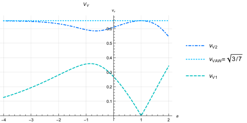
Figure 1: (Color online) Speeds of the two vector modes from eq. (116). The fastest mode (top dot-dashed blue curve) attains the same maximum speed for $a=1$ and for $a\to-\infty$ (top dotted light-blue horizontal line), indicating that the AW value is not exceeded at any value of $a$. Observe that the slowest mode speed (bottom, dashed light blue curve) is zero for $a=1$, so we recover the AW case [47] where only one non-null mode exists.

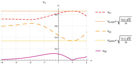
Figure 2: (Color online) Speeds of the three scalar modes from eq. (123). We see that the maximum speed of the fastest mode (top red short-dashed curve) corresponds to the AW solution $a=1$ (top horizontal orange dotted line). The intermediate speed mode (long-dashed orange curve in the middle of the figure) attains its minimum value also at the AW value $a=1$ (bottom horizontal yellow dotted line), and the speeds of this mode never exceed the ones of the fastest mode. These two modes are the generalization of the AW modes found elsewhere. The bottom, single-line purple curve corresponds to the speeds of a new, slowest mode, whose velocity for $a=1$ is zero. Thus we see that the AW case, for which there are only two non-null modes, is consistently included in our formalism.

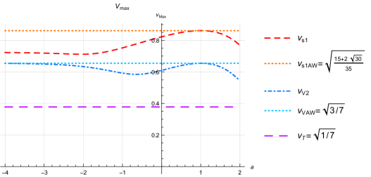
Figure 3: (Color online) Comparison of the maximum propagation speeds of each sector. Top dotted horizontal line corresponds to the AW ($a=1$) scalar mode speed, short-dashed line immediately below corresponds to the velocities of the scalar fastest mode of our model. Middle dotted horizontal line and dot-dashed middle curve correspond respectively to the vector mode speed for AW ($a=1$) and to the speeds of our model. Bottom long-dashed horizontal line is the speed of the tensor mode, which agrees with the AW speed over the entire interval of $a$ values considered. They verify $v_{T}<v_{V}<v_{S}$.

VII Conclusions

The aim of this work was to compute the propagation speeds for a conformal relativistic fluid, assuming hydrodynamics is derived by taking moments of a RTA kinetic equation where the relaxation time becomes a function of momentum, $\tau=\tau_{0}/F[-\beta_{\mu}p^{\mu}]$, suitably modified to make it consistent with energy-momentum conservation. We showed that it is possible to build a kinetic equation within this family which matches any given spectrum for the full Boltzmann equation.

The derivation of hydrodynamics involves assuming a particular parameterization for the 1pdf. We chose the criteria that the parameterized 1pdf should contain the second order Chapman-Enskog solution of the generalized RTA kinetic equation as a special case. Using the moments method we then obtained the sets of the general linear hydrodynamic equations for scalar, vector and tensor perturbations. The choice of which moments to take is determined by the requirement that the dynamics of the perameters enforces positive entropy production.

To analyze a concrete case, we specialized the general equations to the case where $F=\left(\beta_{\mu}p^{\mu}\right)^{a}$, which includes the choices of Anderson-Witting $a=1$ [20, 21] and Marle $a=0$ [18, 19], widely used in the literature, as particular cases. The interpolating values $0\leq a\leq 1$ have already been discussed in the literature [22, 23], motivated by its possible application to improve the description of relativistic heavy ion collisions. Here we have included the full range $-\infty\leq a\leq 2$, which is maximal because larger values of $a$ leads to infrared divergences in the coefficients of the hydrodynamic equations. Allowing for a negative $a$ allows us to explore distributions heavily biased towards hard modes.

We obtained the linearized propagation equations for the tensor, vector and scalar modes and compute the corresponding velocities. The propagation speed is the phase velocity for plane waves in the free streaming limit. Note that though we included the $F$ function through the collision term, taking the free streaming limit does not make it irrelevant, because the chosen parameterization of the 1pdf, dictated by matching to the Chapman-Enskog solution, depends explicitly on $F$.

At the considered order of the 1-PDF the number of tensor, vector and scalar modes are respectively 2, 5 and 6.

For the tensor modes the propagation speed is actually independent of $a$ and agrees with the free streaming Anderson-Witting value [47].

In the vector sector, besides the trivial solution $v_{v}=0$, there are two propagation speeds shown in Fig. (1). There we saw that the fastest propagation speed is bounded above by the Anderson-Witting value [47], which is reached at $a=1$. The slower mode has $v_{v}=0$ for $a=1$. Therefore the number of dynamical vector modes in the Anderson-Witting limit reduces to $3$, as it must.

For the scalar sector we obtained three different propagation speeds as is shown in Fig. (2). As in the tensor and vector sectors, the fastest mode has maximum velocity at $a=1$, where we recover the free streaming Anderson-Witting result [47]. For the intermediate mode we also recover the lower AW speed when $a=1$. The speeds of the slowest mode are significantly lower than the other two scalar modes, and vanishes for $a=1$. In this way we recover the right number od dynamical scalar modes ($4$) in the Anderson-Witting case.

In Fig. (3) we compared the speeds of the three fastest modes. We see that, as expected, they satisfy $v_{T}<v_{v}<v_{s}$ throughout the whole range of $a$ values [39].

We believe that the main contributions of this work are that the theory remains causal for the full range of values of $a$, and that actually the fastest propagation speeds are found in the Anderson-Witting limit $a=1$. Causality is expected because, as we have already said, the theory is built to enforce thermodynamic stability, and it is known that stability, causality and covariance are closely linked [48, 49, 50, 51, 52, 53].

To the best of our knowledge, the fact that the Anderson-Witting RTA [20, 21] produces the fastest propagation speeds is a new result. This has deep implications for the description of strong shocks in relativistic fluids [55], which we expect to elaborate on in a separate contribution.

- [1] P. Romatschke and U. Romatschke, Relativistic Fluid Dynamics In and Out of Equilibrium And Applications to Relativistic Nuclear Collisions, Cambridge Univ. Press, Cambridge, UK (2019).
- [2] E. Calzetta, Real Relativistic Fluids in Heavy Ion Collisions, in Geometric, Algebraic and Topological Methods for Quantum Field Theory; L. Cano, A. Cardona, H. Ocampo, A. F. R. Lega Eds; World Scientific, Singapore, p 155 (2016).
- [3] N. Mirón-Granese, E. Calzetta and A Kandus, Primordial Weibel instability, JCAP 2022, 028 (2022).
- [4] N. Mirón-Granese and E. Calzetta, Primordial Gravitational Waves Amplification from Causal Fluids, Phys. Rev. D 97, 023517 (2018).
- [5] N. Mirón-Granese, Relativistic Viscous Effects on the Primordial Gravitational Waves Spectrum JCAP 2021, 008 (2021).
- [6] L. Rezzolla and O. Zanotti, Relativistic Hydrodynamics (Oxford University Press, Oxford, 2013).
- [7] G. Denicol and D. Rischke, Microscopic Foundations of Relativistic Fluid Dynamics (Springer, Berlin, 2021).
- [8] W. Israel, Nonstationary irreversible thermodynamics: A causal relativistic theory, Ann. Phys. (NY) 100, 310 (1976).
- [9] I. S. Liu, I. Müller and T. Ruggeri, Relativistic thermodynamics of gases, Ann. Phys. 169, 191 (1986).
- [10] R. Geroch and L. Lindblom, Dissipative relativistic fluid theories of divergence type, Phys. Rev. D 41, 1855 (1990).
- [11] J. Peralta-Ramos and E. Calzetta, Divergence-type nonlinear conformal hydrodynamics, Phys. Rev. D 80, 126002 (2009).
- [12] W. Israel and J. M. Stewart, Thermodynamics of nonstationary and transient effects in a relativistic gas, Phys. Lett. A 58, 213 (1976).
- [13] W. Israel and M. Stewart, Transient relativistic thermodynamics and kinetic theory, Ann. Phys. (NY) 118, 341 (1979).
- [14] W. Israel and M. Stewart, On transient relativistic thermodynamics and kinetic theory. II, Proc. R. Soc. London, Ser. A 365, 43 (1979).
- [15] W. Israel and J. M. Stewart, Progress in relativistic thermodynamics and electrodynamics of continuous media, in General Relativity and Gravitation, edited by A. Held, Plenum, New York 2, 491 (1980).
- [16] E. Calzetta and B. L. Hu, Nonequilibrium Quantum Field Theory, Cambridge Univ. Press, Cambridge, UK(2008).
- [17] L. Ciambelli and L. Lehner, Fluid-gravity correspondence and causal first-order relativistic viscous hydrodynamics, Phys. Rev. D 108, 126019 (2023).
- [18] C. Marle, Sur l’etabissement des équations de l’hydrodynamique des fluids relativistes dissipatifs. I. - L’équation de Boltzmann relativiste., Ann. Inst. Henri Poincaré (A), 10, 67 (1969).
- [19] C. Marle, Sur l’etabissement des équations de l’hydrodynamique des fluids relativistes dissipatifs. II. - Méthodes de résolution approchée de l’equation de Boltzmann relativiste., Ann. Inst. Henri Poincaré (A), 10, 127 (1969).
- [20] J. L. Anderson and H. R. Witting, A relativistic Relaxation-Time Model for the Boltzmann Equation, Physica 74, 466 (1974)
- [21] J. L. Anderson and H. R. Witting, Relativistic Quantum Transport Coefficients, Physica 74, 489 (1974).
- [22] K. Dusling, G. D. Moore, and D. Teaney, Radiative energy loss and v 2 spectra for viscous hydrodynamics, Phys. Rev. C 81, 034907 (2010).
- [23] M. Luzum and J.-Y. Ollitrault, Constraining the viscous freeze-out distribution function with data obtained at the BNL Relativistic Heavy Ion Collider (RHIC), Phys. Rev. C 82, 014906 (2010)
- [24] E. Calzetta and J. Peralta-Ramos, Linking the hydrodynamic and kinetic description of a dissipative relativistic conformal theory, Phys. Rev. D 82, 106003 (2010).
- [25] J. Peralta-Ramos and E. Calzetta, Macroscopic approximation to relativistic kinetic theory from a nonlinear closure, Phys. Rev. D 87, 034003 (2013).
- [26] A. Kurkela and U. Wiedemann, Analytic structure of nonhydrodynamic modes in kinetic theory , Eur. Phys. J. C 79, 776 (2019).
- [27] G. Wilka and Z. Włodarczyk, Beyond the relaxation time approximation, Eur. Phys. J. A57 (2021) 221.
- [28] S. Mitra, Relativistic hydrodynamics with momentum-dependent relaxation time , Phys. Rev. C 103, 014905 (2021).
- [29] S. Mitra, Correspondence between momentum-dependent relaxation time and field redefinition of relativistic hydrodynamic theory, Phys. Rev. C 105, 014902 (2022).
- [30] G. Rocha, G. Denicol and J. Noronha, Novel Relaxation Time Approximation to the Relativistic Boltzmann Equation , Phys. Rev. Lett. 127, 042301 (2021).
- [31] G. Rocha, M. Ferreira, G. Denicol and J. Noronha, Transport coefficients of quasiparticle models within a new relaxation time approximation of the Boltzmann equation, Phys. Rev. D 106, 036022 (2022).
- [32] V. Ambruş and E. Molnár, Shakhov-type extension of the relaxation time approximation in relativistic kinetic theory and second-order fluid dynamics, eprint arXiv:2311.11603.
- [33] V. Ambruş and E. Molnár,High-order Shakhov-like extension of the relaxation time approximation in relativistic kinetic theory , eprint arXiv:2401.04017
- [34] J. Hu, Full-order mode analysis within a mutilated relaxation time approximation, eprint arXiv:2310.05606
- [35] D. Dash, S. Bhadury, S. Jaiswal and A. Jaiswal, Extended relaxation time approximation and relativistic dissipative hydrodynamics, Phys. Lett. B, 831, 13720 (2022).
- [36] D. Dash, S. Bhadury, S. Jaiswal and A. Jaiswal, Relativistic second-order viscous hydrodynamics from kinetic theory with extended relaxation-time approximation, Phys. Rev. C 108, 064913 (2023).
- [37] T. Bhattacharyya, Non-extensive Boltzmann Transport Equation: the Relaxation Time Approximation and Beyond, Physica A 624, 128910 (2023).
- [38] H. Struchtrup, Macroscopic Transport Equations for Rarefied Gas Flows (Springer, Berlin, 2005).
- [39] G. Boillat and T. Ruggeri, Relativistic gas: Moment equations and maximum wave velocity, J. Math. Phys. (N.Y.) 40, 6399 (1999).
- [40] L. Cantarutti and E. Calzetta, Dissipative-type theories for Bjorken and Gubser flows, Int. J. Mod. Phys. A 35, 2050074 (2020).
- [41] G. Rocha, D. Wagner, G. Denicol, J. Noronha, and D. Rischke, D.H. Theories of Relativistic Dissipative Fluid Dynamics. Entropy 26, 189 (2024).
- [42] M. Strickland, Hydrodynamization and resummed viscous hydrodynamics, arXiv:2402.09571, Contributed chapter to Quark-Gluon Plasma 6 book
- [43] S. Chapman and T. G. Cowling, The Mathematical Theory of Non-Uniform Gases, 3rd. ed. ,Cambridge Univ. Press, Cambridge (1970).
- [44] S. Bhadury, M. Kurian, V. Chandra and A. Jaiswal, First order dissipative hydrodynamics and viscous corrections to the entropy four-current from an effective covariant kinetic theory, J. Phys. G 47 (2020) 8, 085108
- [45] S. Bhadury, M. Kurian, V. Chandra and A. Jaiswal, Second order relativistic viscous hydrodynamics within an effective description of hot QCD medium, J. Phys. G: 48, 105104, (2021).
- [46] S. Diles, A. Miranda, L. Mamani, A. Echemendia and V. Zanchin, Third-order relativistic fluid dynamics at finite density in a general hydrodynamic frame, arXiv:2311.01232.
- [47] G. Perna and E. Calzetta, Linearized dispersion relations in viscous relativistic hydrodynamics, Phys. Rev. D 104, 096005 (2021).
- [48] S. Mitra, Causality and stability analysis of first-order field redefinition in relativistic hydrodynamics from kinetic theory, Phys. Rev. C 105, 054910 (2022).
- [49] M. Heller, A. Serantes, M. Spaliński and B. Withers, The Hydrohedron: Bootstrapping Relativistic Hydrodynamics, arXiv:2305.07703v2
- [50] N. Abboud, E. Speranza and J. Noronha, Causal and stable first-order chiral hydrodynamics , arXiv:2308.02928.
- [51] C. de Brito, G. Rocha and G. Denicol, Hydrodynamic theories for a system of weakly self-interacting classical ultra-relativistic scalar particles: causality and stability , arXiv:2311.07272.
- [52] R. Hoult and P. Kovtun, Causality and classical dispersion relations, Phys. Rev. D 109 (2024) 4, 046018.
- [53] D-L Wang and S. Pu, Stability and causality criteria in linear mode analysis: stability means causality, Phys. Rev. D 109, L031504 (2024).
- [54] W. Israel, Relativistic theory of shock waves, Proc. R. Soc. A 259, 129 (1960).
- [55] E. Calzetta, Steady asymptotic equilibria in conformal relativistic fluids, Phys. Rev. D 105, 036013 (2022).
- [56] W. Israel, Covariant fluid mechanics and thermodynamics: An introduction, in A. M. Anile and Y. Choquet-Bruhat (eds.) Relativistic Fluid Dynamics(Springer, New York, 1988), p. 152.
- [57] W. Israel, The relativistic Boltzmann equation. In: L. O’Raifeartaigh (ed.), General Relativity: Papers in Honour of J. L. Synge, pp. 201–241. Clarendon, Oxford (1972).
- [58] S. R. de Groot, W. A. van Leeuwen, and C. G. van Weert, Relativistic Kinetic Theory (North-Holland, Amsterdam, 1980).
- [59] J. M. Stewart, Non-Equilibrium Relativistic Kinetic Theory (Springer, New York, 1971).
- [60] R. Liboff, Kinetic Theory (Springer, New York, 2003).
- [61] C. Cercignani and G. Medeiros Kremer, The Relativistic Boltzmann Equation: Theory and Applications (Birkhauser, Basel, 2002).
- [62] M. Dudyński, Spectral properties of the linearized Boltzmann operator in Lp for , J. Stat. Phys. 153, 1084 (2013).
- [63] L. Luo and H. Yu, Spectrum analysis of the linearized relativistic Landau equation, J. Stat. Phys. 163, 914 (2016).
- [64] C. Eckart, The Thermodynamics of Irreversible Processes. III. Relativistic Theory of the Simple Fluid, Phys. Rev. 58, 919 (1940)
- [65] L. D. Landau and E. M. Lifshitz, Fluid Mechanics, Pergamon Press, Oxford (1959).