Kinetic theories of state- and generation-dependent cell populations

Abstract

We formulate a general, high-dimensional kinetic theory describing the internal state (such as gene expression or protein levels) of cells in a stochastically evolving population. The resolution of our kinetic theory also allows one to track subpopulations associated with each generation. Both intrinsic noise of the cell’s internal attribute and randomness in a cell’s division times (demographic stochasticity) are fundamental to the development of our model. Based on this general framework, we are able to marginalize the high-dimensional kinetic PDEs in a number of different ways to derive equations that describe the dynamics of marginalized or “macroscopic” quantities such as structured population densities, moments of generation-dependent cellular states, and moments of the total population. We also show how nonlinear “interaction” terms in lower-dimensional integrodifferential equations can arise from high-dimensional linear kinetic models that contain rate parameters of a cell (birth and death rates) that depend on variables associated with other cells, generating couplings in the dynamics. Our analysis provides a general, more complete mathematical framework that resolves the coevolution of cell populations and cell states. The approach may be tailored for studying, e.g., gene expression in developing tissues, or other more general particle systems which exhibit Brownian noise in individual attributes and population-level demographic noise.

I Introduction

Mathematical models have been formulated to describe the evolution of populations according to a number of individual attributes such as age, size, and/or added size since birth. Such structured population models have various applications across diverse fields. For example, deterministic age-structured models that incorporate age-dependent birth and death were developed by McKendrick and have been applied to human populations [1, 2]. Structured population models have also been applied to model cell size control [3, 4], cellular division mechanisms [5], and structured cell population models [6, 7].

In a proliferating cell population, individual cell growth is interrupted by cell division events that generate daughter cells. Kinetic theory is a natural framework to capture the link between individual cellular growth and division, within a proliferating population of cells. Kinetic theories of simple birth-death processes that track the chronological age of each cell have been developed [8, 9, 10, 11] that establish a rigorous mathematical framework to describe how individual cell aging, growth, and division affect population-level quantities such as population-averaged cell size. The kinetic theory PDE can be marginalized in different ways and reduce, in different limits, to master-like equations or structured population-like PDEs, thus unifying deterministic “moment” equations (the structured population PDEs) with Markovian birth-death-like models. Stochastic fluctuations in parameters such as the cellular growth rate have also been included [12], but integrating fluctuations of internal variables with random birth-death events (demographic stochasticity) is challenging due to the combinatorial complexity and unwieldiness of the relevant equations.

Besides simple individual-cell dynamical variables such as cell age or cell size, gene (mRNA) or protein expression levels are also measured cellular attributes that are important in cell biology, particularly during development. Since there are many different species of mRNA or proteins, the expression pattern is a vector of fluctuating variables.

Although modern computational and statistical techniques can be used to quantitatively infer single cellular mRNA [13] or protein [14, 15] levels from experimental data, mathematical models of how expression levels or cell states evolve is often couched in terms of transport along Waddington or fitness landscapes [16, 17]. The value of the landscape may represent an “energy” function that is shaped by different genes, or a proliferation rate that is a function different gene expression rates. However, how populations of cells are represented in such high-dimensional “landscapes” is unclear. Moreover, since cellular division rates and death rates typically depend in depend on internal stochastic cell variables such as gene expression levels [18, 19, 20], it is important to model how fluctuating-gene-expression-dependent birth or death rates feature in the evolution of a population along an appropriate landscape.

Kinetic models have the capability of precisely describing both the stochastic dynamics of individual cell states and the stochastic birth-death processes associated with an evolving population. Not only is the coupling between individual cell states and the evolution of the population explicit in a kinetic equation, but potential functions governing intracell state dynamics and proliferation (defining a fitness function) arise naturally in the kinetic framework.

Previously derived kinetic models such as the timer-sizer model for cell populations distributed across size [21, 10] incorporate stochastic differential equations (SDEs) to track the dynamics individual internal cell states such as size or mRNA/protein levels. Marginalization of the kinetic equations results in equations for the correlation functions that explicitly show how individual cell states are linked to key macroscopic quantities of the overall population. However, these kinetic theories could not track lineages or generational subpopulations of cells nor did they incorporate cell death or cell division that may also depend on other stochastic variables associated with the cell.

In this paper, we formally develop a complete kinetic model that tracks continuous-valued, stochastically evolving variables (e.g., gene expression, cellular size, mRNA level, protein level, etc.) and the discrete generation number of each cell. The mathematical framework we use for delineating cell of differernt attribute values across different generations shares a related structure to one recently used to describe ages across different cell stages [11]. In our problem, noise in gene expression is described by a continuous-time stochastic process while noise in division events is described by a Markov jump process. Our model couples these stochastic processes through an SDE-jump-process hybrid model in which the division and death rates explicitly depend on fluctuating gene expression levels [22, 23]. All of these quantities are tracked along different generations. The mathematical framework we use for delineating cell of differernt attribute values across different generations shares a related structure to one recently used to describe ages across different cell stages [11].

In the next section, we define the kinetic model and show how potentials that govern the intracellular dynamics and the population fitness can be motivated. Since the development of our generation-dependent kinetic equations requires intensive book-keeping and associated notation to resolve the time-dependent attributes of each member of the entire population, many of the steps are detailed in extensive mathematical Appendices. However, eventually, in Section III we marginalize our high-dimensional kinetic PDE to derive a number of more meaningful “reduced” equations that describe the evolution of key quantities of biological interest. These new results are summarized and listed in the Summary and Conclusions. We also carry out a numerical experiment on a simple example to show how cellular gene expression levels evolve over generations and how the macroscopic cellular density (with respect to gene expression level), when interrupted by cellular division, can be prevented from returning to the equilibrium distribution. In the Conclusions, we discuss potential applications and extensions.

II Kinetic equation formulation

For simplicity, we first assume the internal state of each cell is characterized by a one-dimensional scalar quantity $X\in\mathbb{R}$. This continuous stochastic variable may represent, for example, the expression level of a single mRNA transcript or protein abundance (or log-abundance). Besides this continuous variable, associated with each cell is the discrete generation $i\in\mathbb{N}^{+}$ to which it belongs (assuming it is part of a lineage derived from an ancestor). We model the evolution of $X_{i,j}$ (the internal state of the $j^{\text{th}}$ cell in the $i^{\text{th}}$ generation) using an SDE of the standard form [24, 25]

$$\textrm{d}X_{i,j}(t)=g_{i,j}(X_{i,j},t)\textrm{d}{t}+\sigma_{i,j}(X_{i,j},t)\textrm{d}W_{i,j},$$ (1)

where $g_{i,j}(X_{i,j},t)\textrm{d}{t}$ is the deterministic convection that depends on both $X_{i,j}$ and the generation $i$, and $\textrm{d}W_{i,j}$ are increments of independent Wiener processes for each $i,j$. Thus, the term $\sigma_{i,j}(X_{i,j},t)\textrm{d}W_{i,j}$ represents the “intrinsic” fluctuation in the evolution of $X_{i,j}(t)$. Often, one can assume that the convection arises from gradients of a potential “energy function” $\Phi$: $g_{i,j}(X_{i,j},t)\coloneqq-\nabla\Phi(x,t)|_{x=X_{i,j}}$ [17]. Although a gradient of $\Phi(x,t)$ may conveniently describes a time-dependent force that changes gene expression, nonconservative driving with metabolically driven fluxes, which cannot be described by a potential, is also to be expected [26].

We assume that both $g_{i}$ and $\sigma_{i}$ are Lipschitz continuous so the solution $X_{i,j}(t)$ of Eq. (1) exists and is almost surely unique given any initial condition $X_{i,j}(0)$. The evolution of $X_{i,j}$ is interrupted by the cell division; an $i^{\text{th}}$ generation cell with internal state $X_{i,j}$ divides in time $\textrm{d}t$ with total probability $\beta_{i}(X_{i,j})\textrm{d}t$. This Markovian birth rate can be further stratified by internal state of the two resulting daughter cells immediately after their birth. We denote the differential birth rate density of producing one daughter with internal state $X_{1}$ and the other with state $X_{2}$ as $\tilde{\beta}_{i,j}(X_{i,j},X_{1},X_{2})$. Integrating over all possible daughter cell states $X_{1},X_{2}$ defines the total division rate:

$$\int\tilde{\beta}_{i,j}(X_{i,j},X_{1},X_{2})\textrm{d}{X}_{1}\textrm{d}{X}_{2}=\beta_{i,j}(X_{i,j}).$$ (2)

A form for $\tilde{\beta}$ might be

$$\tilde{\beta}_{i,j}(X_{i,j},X_{1},X_{2})\propto e^{-\phi(X_{1},X_{2}|X_{i,j})},$$ (3)

which defines a “free energy” function $\phi(X_{1},X_{2}|X_{i,j})$ for the rate of a mother cell with attribute value $X$ to divide into daughters cell with attribute values $X_{1}$ and $X_{2}$. If the states of the daughter cells tend towards being similar in value to that of their mother cell, then $\phi(X_{1},X_{2}|X_{i,j})$ would exhibit a minimum at $X_{1},X_{2}\approx X$. Although $\Phi$ and $\phi$ might be loosely described in terms of Waddington and fitness landscapes, our unifying kinetic framework allows them to be unambiguously described in terms of the intracellular advection $g_{i,j}(X_{i,j},t)$ and proliferation function $\tilde{\beta}$, respectively.

Since the derivation of our kinetic theory requires the use of a number of variables and indices, we define some simplifying notation. Specifically, each of the $n_{i}$ elements of the bold vector $\bm{X}_{i}$ represents the expression level $X_{i,j}$ of the $j^{\rm th},\,1\leq j\leq n_{i}$ cell in the $i^{\rm th}$-generation subpopulation. These vectors $\bm{X}_{i}$ for the subpopulations across generations $1\leq i\leq k$ can be collected as a matrix defined as $\bm{X}_{\bm{n}}\coloneqq(\bm{X}_{1},\ldots,\bm{X}_{k})$, where $\bm{n}\coloneqq(n_{1},...,n_{k})$ is a vector representing the total number of cells in each generation $1\leq i\leq k$. Each value $n_{i}$ evolves stochastically defined by random birth and death events. Below is a table of the various definitions and overall notation used throughout this paper.

Symbol	Definition and explanation
$\bm{n}(t)$	$\bm{n}(t)\coloneqq(n_{1}(t),...,n_{k(t)}(t))$: time-dependent vector of random numbers of cells in the $i^{\text{th}}$ generation, $i=1,...,k$
$\bm{n}$	$\bm{n}\coloneqq(n_{1},...,n_{k})$: vector of integer values $n_{i}$ of the number of cells in generation $i=1,...,k$
$\bm{X}(t)_{\bm{n}(t)}$	$\bm{X}(t)_{\bm{n}(t)}\coloneqq(\bm{X}_{1}(t),...,\bm{X}_{k(t)}(t))$, $\bm{X}_{i}(t)\coloneqq(X_{i,1}(t),...,X_{i,n_{i}(t)}(t))$: time-dependent random variable describing the state of each cell, e.g., gene expression level $X_{i,n_{i}(t)}$ of the $n_{i}^{\rm th}$ cell in the $i^{\rm th}$ generation
$\bm{X}_{\bm{n}}$	$\bm{X}_{\bm{n}}\coloneqq(\bm{X}_{1},...,\bm{X}_{k})$, $\bm{X}_{i}\coloneqq(X_{i,1},...,X_{i,n_{i}})$: values of $\bm{X}(t)_{\bm{n}(t)}$
$\vec{X}_{n}$	$\vec{X}_{n}\coloneqq(X_{1},...,X_{n})$, the vector of state values for any collection of $n$ cells
$g_{i,j}(X_{i,j},t)$	deterministic growth rate of the $j^{\text{th}}$ cell in the $i^{\text{th}}$ generation
$\sigma_{i,j}(X_{i,j},t)$	noise in the growth of the $j^{\text{th}}$ cell in the $i^{\text{th}}$ generation
$\beta_{i,j}(X_{i,j})$	division rate of the $j^{\text{th}}$ cell in the $i^{\text{th}}$ generation
$\mu_{i,j}(X_{i,j})$	death rate of the $j^{\text{th}}$ cell in the $i^{\text{th}}$ generation
$\tilde{\beta}_{i,j}(X_{i,j},X_{1},X_{2})$	differential division rate of the $j^{\text{th}}$ cell in the $i^{\text{th}}$ generation into two cells in the $(i+1)^{\text{th}}$ generation with states $X_{1},X_{2}$
$\bm{X}_{\bm{n}_{\text{b},-i}}^{{-j}}$	states of the cell population right after the $j^{\text{th}}$ cell in the $i^{\text{th}}$ generation divides. $\bm{X}_{\bm{n}_{\text{b},-i}}^{{-j}}$ differs from $\bm{X}_{\bm{n}}$ in that the state variables for the cells in the $(i-1)^{\text{th}}$ generation is $(X_{i-1,1},...,X_{i-1,j-1},X_{i-1,j+1},...X_{i-1,n_{i}})$ and the state variables for the cells in the $i^{\text{th}}$ generation are $(X_{i,1},...,X_{i,n_{i}},X_{1},X_{2})$
$\bm{X}^{-j}_{\bm{n}_{\text{d},-i}}$	states of the cell population right after the $j^{\text{th}}$ cell in the $i^{\text{th}}$ generation dies. $\bm{X}^{-j}_{\bm{n}_{\text{d},-i}}$ differs from $\bm{X}_{\bm{n}}$ in that the state variables for the cells in the $(i-1)^{\text{th}}$ generation are $(X_{i-1,1},...,X_{i-1,j-1},X_{i-1,j+1},...X_{i-1,n_{i}})$
$\bm{X}_{\bm{n}_{\text{b},i-1}}^{j}$	pre-division cellular population: it differs from $\bm{X}_{\bm{n}}$ in that the state variables for the cells in the $(i-1)^{\text{th}}$ generation is $(X_{i-1,1},...,X_{i-1,j-1},Y,X_{i-1,j},...)$ and the state variables for the cells in the $i^{\text{th}}$ generation are $(X_{i,1},...,X_{i,n_{i}-2})$ (an additional cell with $Y$ in the $(i-1)^{\text{th}}$ generation divides and gives birth to two new daughter cells $X_{i,n_{i}-1},X_{i,n_{i}}$ in the $i^{\text{th}}$ generation)
$\bm{X}_{\bm{n}_{\text{d},i}}^{j}$	pre-death cell population states. This differs from $\bm{X}_{\bm{n}}$ in that the state variables for the cells in the $i^{\text{th}}$ generation are $(X_{i,1},...,X_{i,j-1},Y,X_{i,j},...)$ (an additional cell in the $i^{\text{th}}$ generation with $Y$ dies)
$\bm{X}_{\bm{n}_{\text{b},i}}^{j_{1},j_{2}}$	pre-division state which differs from $\bm{X}_{\bm{n}}$ in that the state vector associated with the $i^{\text{th}}$ generation is $(Y,X_{i,1},...X_{i,n_{i}})$ and the state of the $(i+1)^{\text{th}}$ generation does not contain components $X_{i+1,j_{1}}$ and $X_{i+1,j_{2}}$

Table 1: Overview of variables. A list of the main variables and parameters used. The specific labels and definitions of state vectors given provide the proper bookkeeping of all possible initial and final states upon birth and death.

Next, define $p_{\bm{n}}(\bm{X}_{\bm{n}},t|\bm{X}(0)_{\bm{n}(0)},0)$ as the probability density function that the population has $\bm{n}$ cells with internal states $\bm{X}_{\bm{n}}$ given the initial condition that the system has $\bm{n}(0)$ cells with internal state values $\bm{X}(0)_{\bm{n}(0)}$ at $t=0$. For notational simplicity, we name the cell state random variables (at time $t$) $X_{i,j}(t),\bm{X}_{i}(t)$, and $\bm{X}(t)_{\bm{n}(t)}$, and denote their values by and $X_{i,j},\bm{X}_{i}$, and $\bm{X}_{\bm{n}}$, respectively. The probability density $p_{\bm{n}}(\bm{X}_{\bm{n}},t|\bm{X}(0)_{\bm{n}(0)},0)$ can be defined as the expectation over trajectories from ($\bm{X}(0)_{\bm{n}(0)},0$) to ($\bm{X}_{\bm{n}},t$):

$$p_{\bm{n}}\big{(}\bm{X}_{\bm{n}},t|\bm{X}(0)_{\bm{n}(0)},0\big{)}=\begin{cases}\begin{aligned} &\mathbb{E}\Big{[}\delta\big{(}\bm{X}(t)_{\bm{n}(t)}-\bm{X}_{\bm{n}}\big{)}S\big{(}t;\bm{X}(t)_{\bm{n}(t)}\big{)}\Big{|}\bm{X}(0)_{\bm{n}(0)},0;\bm{n}(0<s<t)=\bm{n}(0)\Big{]},\quad\,\,\bm{n}=\bm{n}(0)\\[-6.0pt] &\hskip 5.69054pt+\!\int_{0}^{t}\!\mathbb{E}\Big{[}\tilde{J}\big{(}t,\tau;\bm{X}(t)_{\bm{n}(t)},\bm{n}(0)\big{)}S\big{(}\tau;\bm{X}(\tau)_{\bm{n}(\tau)}\big{)}\Big{|}\bm{X}(0)_{\bm{n}(0)},0;\bm{n}(0<s<\tau)=\bm{n}(0)\Big{]}\textrm{d}\tau,\\[12.0pt] &\displaystyle\mathbb{E}\Big{[}\int_{0}^{t}\tilde{J}(t,\tau;\bm{X}(0)_{\bm{n}(0)},\bm{n}(0))S\big{(}\tau;\bm{X}(\tau)_{\bm{n}(\tau)}\big{)}\,\textrm{d}\tau\Big{|}\bm{X}(0)_{\bm{n}(0)},0\Big{]},\qquad\qquad\quad\,\,\bm{n}\neq\bm{n}(0)\end{aligned}\end{cases}$$ (4)

where

$$S\big{(}t;\bm{X}(t)_{\bm{n}(t)}\big{)}\equiv \exp\Big{[}-\!\int_{0}^{t}\sum_{i=1}^{k(0)}\sum_{j=1}^{n_{i}(0)}\Big{(}\beta\big{(}X_{i,j}(s)\big{)}+\mu\big{(}X_{i,j}(s)\big{)}\Big{)}\textrm{d}s\Big{]}$$ (5)

$$\tilde{J}\big{(}t,\tau;\bm{X}_{\bm{n}},\bm{n}(0)\big{)}\equiv \sum_{i=1}^{k(0)}\sum_{j=1}^{n_{i}(0)}\Big{[}\tilde{\beta}_{i,j}\big{(}X_{i,j}(\tau),X_{1}(\tau),X_{2}(\tau)\big{)}p_{\bm{n}}(\bm{X}_{\bm{n}},t-\tau|\bm{X}(\tau)_{\bm{n}(0)_{\text{b},-i}}^{-j},0)$$

$$\qquad\hskip 85.35826pt+\mu_{i,j}\big{(}X_{i,j}(\tau)\big{)}p_{\bm{n}}(\bm{X}_{\bm{n}},t-\tau|\bm{X}(\tau)_{\bm{n}(0)_{\text{d},-i}}^{-j},0)\Big{]}.$$

Definitions of $\bm{X}^{-j}_{\bm{n}(0)_{\text{b},-i}}(s)$ and $\bm{X}^{-j}_{\bm{n}(0)_{\text{d},-i}}$ are given in Table 1. The term $S\big{(}t;\bm{X}(t)_{\bm{n}(t)}\big{)}$ represents the survival probability up to time $t$ while $\tilde{J}(t,\tau;\bm{X}(t)_{\bm{n}(t)},\bm{n}(0))$ describes the probability flux from a given state $\bm{X}(\tau)_{\bm{n}(\tau)}$ to the current state $\bm{X}(t)_{\bm{n}(t)}$ due to division or death at time $\tau$. The first form on the RHS of Eq. (4) is the probability that no division or death happens in the system during time $[0,t]$ and the final internal states of the cell population are $\bm{X}(t)_{\bm{n}(t)}$ while the second form in Eq. (4) denotes the probability that at least one division or death happened within $[0,t]$ to arrive at the final internal state $\bm{X}(t)_{\bm{n}(t)}$.

We shall show that under certain conditions, $p_{\bm{n}}(\bm{X}_{\bm{n}},t|\bm{X}(0)_{\bm{n}(0)},0)$ satisfies the partial differential equation

$$\frac{\partial p_{\bm{n}}}{\partial t}+\sum_{i=1}^{k}\sum_{j=1}^{n_{i}}\frac{\partial(g_{i,j}p_{\bm{n}})}{\partial X_{i,j}}= \mfrac{1}{2}\sum_{i=1}^{k}\sum_{j=1}^{n_{i}}\frac{\partial^{2}(\sigma_{i,j}p_{\bm{n}})}{(\partial X_{i,j})^{2}}-\sum_{i=1}^{k}\sum_{j=1}^{n_{i}}\big{(}\beta_{i,j}(X_{i,j})+\mu_{i,j}(X_{i,j})\big{)}p_{\bm{n}}$$ (6)

$$+\sum_{i=2}^{k}\sum_{j=1}^{n_{i-1}+1}\!\int\!\tilde{\beta}(Y,X_{i,n_{i}-1},X_{i,n_{i}})p_{\bm{n}_{\text{b},i-1}}(\bm{X}^{j}_{\bm{n}_{\text{b},i-1}},t|\bm{X}(0)_{\bm{n}(0)},0)\,\textrm{d}{Y}$$

$$+\sum_{i=1}^{\infty}\sum_{j=1}^{n_{i}+1}\!\int\!\mu(Y)p_{\bm{n}_{\text{d},i}}(\bm{X}^{j}_{\bm{n}_{\text{d},i}},t|\bm{X}(0)_{\bm{n}(0)},0)\,\textrm{d}{Y}.$$

In Eq. (6), the pre-division cell population $\bm{X}_{\bm{n}_{\text{b},i-1}}^{{j}}$ and the pre-death cell population $\bm{X}_{\bm{n}_{\text{d},i}}^{{j}}$ are explicitly defined in Table 1. The mathematical steps and necessary conditions needed to show that $p_{\bm{n}}(\bm{X}_{\bm{n}},t|\bm{X}(0)_{\bm{n}(0)},0)$ defined in Eq. (4) satisfies Eq. (6) is given in Appendix A. We impose the normalization condition $\sum_{{\bm{n}}}\int p_{\bm{n}}(\bm{X}_{\bm{n}},t|\bm{X}(0)_{\bm{n}(0)},0)\textrm{d}{\bm{X}_{\bm{n}}}=1$ for every $\bm{X}(0)_{\bm{n}(0)}$ and average over an initial distribution of $\bm{X}(0)_{\bm{n}(0)}(0)$ (denoted by $q_{\bm{n}(0)}(\bm{X}(0)_{\bm{n}(0)},0)$) to define an unconditional probability density

$$p_{\bm{n}}(\bm{X}_{\bm{n}},t)\coloneqq\sum_{\bm{n}(0)}\int_{\bm{X}_{\bm{n}(0)}}\!\!p_{\bm{n}}(\bm{X}_{\bm{n}},t|\bm{X}(0)_{\bm{n}(0)},0)q_{\bm{n}(0)}(\bm{X}(0)_{\bm{n}(0)},0)\,\textrm{d}\bm{X}(0)_{\bm{n}(0)}$$ (7)

that also satisfies Eq. (6).

Next, we define the symmetric probability density distribution

$$\rho_{\bm{n}}(\bm{X}_{\bm{n}},t)\coloneqq\prod_{i=1}^{k}\frac{1}{n_{i}!}\sum_{\pi}p_{\bm{n}}(\pi(\bm{X}_{\bm{n}}),t)$$ (8)

where $p_{\bm{n}}$ is defined in Eq. (7) and $\pi(\bm{X}_{\bm{n}})$ is a permutation operator that reorders the sequence of the state variables $X_{i,j}$ of cells within each generation, for all generations. Thus, the summation is taken over all such grouped permutations ($\prod_{i=1}^{k}{n_{i}!}$ permutations in total). In the special case

$$g_{i,j}=g_{i},\,\sigma_{i,j}=\sigma_{i},\,\beta_{i,j}=\beta_{i},\,\mu_{i,j}=\mu_{i},\,\tilde{\beta}_{i,j}=\tilde{\beta}_{i},$$ (9)

i.e., when the rate parameters depend at most on the generation of a cell, $\rho_{\bm{n}}(\bm{X}_{\bm{n}},t)$ defined in Eq. (8) obeys

$$\frac{\partial\rho_{\bm{n}}}{\partial t}+\sum_{i=1}^{k}\sum_{j=1}^{n_{i}}\frac{\partial(g_{i}\rho_{\bm{n}})}{\partial X_{i,j}}= \mfrac{1}{2}\sum_{i=1}^{k}\sum_{j=1}^{n_{i}}\frac{\partial^{2}(\sigma_{i,j}\rho_{\bm{n}})}{(\partial X_{i,j})^{2}}-\sum_{i=1}^{k}\sum_{j=1}^{n_{i}}\big{(}\beta_{i,j}(X_{i,j})+\mu_{i,j}(X_{i,j})\big{)}\rho_{\bm{n}}$$ (10)

$$+\sum_{i=1}^{k-1}\frac{n_{i}+1}{n_{i+1}(n_{i+1}-1)}\!\sum_{1\leq j_{1}\neq j_{2}\leq n_{i+1}}\!\!\!\medint\int\tilde{\beta}_{i}(Y,X_{i+1,j_{1}},X_{i+1,j_{2}})\rho_{\bm{n}_{\text{b},i}}(\bm{X}_{\bm{n}_{\text{b},i}}^{{j_{1},j_{2}}},t)\,\textrm{d}{Y}$$

$$+\sum_{i=1}^{\infty}\sum_{j=1}^{n_{i}+1}\!\int\!\mu_{i}(Y)\rho_{\bm{n}_{\text{d},i}}(\bm{X}_{\bm{n}_{\text{d},i}}^{{j}},t)\,\textrm{d}{Y},$$

where $\bm{X}_{\bm{n}_{\text{b},i}}^{j_{1},j_{2}}$ differs from $\bm{X}_{\bm{n}}$ in that the state vector associated with cells in the $i^{\text{th}}$ generation are $(Y,X_{i,1},...X_{i,n_{i}})$ and the state vector for cells in the $(i+1)^{\text{th}}$ generation does not have the components $X_{i+1,j_{1}}$ and $X_{i+1,j_{2}}$.

Finally, in many systems, the state variable is a multi-dimensional vector instead of a scalar, i.e., $X_{i,j}\coloneqq(X_{i,j,1},...,X_{i,j,d})\in\mathbb{R}^{d}$ may also represent $d$ different gene or protein expression levels in the $j^{\text{th}}$ cell in the $i^{\text{th}}$ generation. This vector may represent, for example, $d$ different gene or protein expression levels. We assume that the evolution of $X_{i,j}$ (each element now implicitly a vector of attributes) follows the Brownian SDE

$$\textrm{d}X_{i,j}=\bm{g}_{i,j}(X_{i,j},t)\textrm{d}{t}+\bm{\Sigma}_{i,j}(X_{i,j},t)\textrm{d}\bm{W}_{i,j}$$ (11)

where $\bm{W}_{i,j}$ is a $d_{0}$-dimensional vector of independent Wiener processes ($d_{0}\leq d$) for each $i,j$ and the coefficients $\bm{g}_{i,j}(X_{i,j},t)\coloneqq(g_{i,j,1}(X_{i,j},t),...,g_{i,j,d}(X_{i,j},t)):\mathbb{R}^{d}\times\mathbb{R}^{+}\rightarrow\mathbb{R}^{d},\big{(}\bm{\Sigma}_{i,j}\big{)}_{mn}\coloneqq\big{(}\sigma_{i,j}(X_{i,j},t)\big{)}_{mn}:\mathbb{R}^{h}\times\mathbb{R}^{+}\rightarrow\mathbb{R}^{d\times d_{0}},m=1,...,d,n=1,...,d_{0}$ are all smooth, uniform Lipschitz continuous, and uniform bounded. We can also define the symmetric probability density distribution $\rho_{\bm{n}}(\bm{X}_{\bm{n}},t)$ as in Eqs. (8) and after applying the multi-dimensional forward Feynman-Kac equation case in [27] we can show that the differential equation satisfied by such $\rho_{\bm{n}}$ is

$$\frac{\partial\rho_{\bm{n}}}{\partial t}+\sum_{i=1}^{k}\sum_{j=1}^{n_{i}}\sum_{\ell=1}^{d}\frac{\partial(g_{i,j,\ell}\rho_{\bm{n}})}{\partial X_{i,j,\ell}}= \mfrac{1}{2}\sum_{i=1}^{k}\sum_{j=1}^{n_{i}}\sum_{\ell_{1},\ell_{2}=1}^{d}\!\!\frac{\partial^{2}(\sum_{h=1}^{d_{0}}(\Sigma_{i,j})_{\ell_{1},h}(\Sigma_{i,j})_{\ell_{2},h}\,\rho_{\bm{n}})}{(\partial X_{i,j,\ell_{1}}\partial X_{i,j,\ell_{2}})}$$ (12)

$$\,\,-\sum_{i=1}^{k}\sum_{j=1}^{n_{i}}\big{(}\beta_{i,j}(X_{i,j})+\mu_{i,j}(X_{i,j})\big{)}\rho_{\bm{n}}$$

$$\,\,\sum_{i=1}^{k-1}\frac{n_{i}+1}{n_{i+1}(n_{i+1}-1)}\!\sum_{1\leq j_{1}\neq j_{2}\leq n_{i+1}}\!\!\!\!\!\medint\int\tilde{\beta}(Y,X_{i+1,j_{1}},X_{i+1,j_{2}})\rho_{\bm{n}_{\text{b},i}}(\bm{X}_{\bm{n}_{\text{b},i}}^{j_{1},j_{2}},t)\,\textrm{d}{Y}$$

$$\,\,+\sum_{i=1}^{\infty}\sum_{j=1}^{n_{i}+1}\medop\int\mu_{i,j}(Y)\rho_{\bm{n}_{\text{d},i}}(\bm{X}_{\bm{n}_{\text{d},i}}^{j},t)\,\textrm{d}{Y}$$

if the coefficients $\beta_{i,j}=\beta_{i},\mu_{i,j}=\mu_{i},\tilde{\beta}_{i,j}=\tilde{\beta}_{i}$ are homogeneous for cells in the same generation.

In Appendix C, we also derive kinetic equations for the population density associated with cells that are also labeled by their age. The derivation assumes the budding model of birth where on daughter cell’s age is set to zero immediately after birth [8, 9].

III Mass-action differential equations

Henceforth, we will consider the “simpler” single-gene model. Extension to $d$-dimensional attributes can be implemented following the structure in Eqs. (11) and (12).

Through marginalization of the kinetic equation (10) we can derive he differential equations that describe the evolution of certain “macroscopic” quantities such as the expected total-population levels of $X$. In this section, we derive governing equations for examples of macroscopic quantities by marginalizing Eq. (10), which are then solved numerically to show how quantities such as cellular gene expression levels can evolve over generations.

III.1 Evolution of the population density

First, we can track the marginal cell distributions of certain cells in specified generations by defining the macroscopic quantity

$$u_{\bm{n}}(\bm{X}_{\bm{n}},t)\coloneqq\!\sum_{\bm{m}\geq\bm{n}}\prod_{\ell=1}^{\infty}(\bm{m}_{\ell})_{\bm{n}_{\ell}}\int_{\bm{X}_{\bm{m}\backslash\bm{n}}}\!\!\!\rho_{\bm{m}}(\bm{X}_{\bm{m}},t)\textrm{d}\bm{X}_{\bm{m}\backslash\bm{n}},$$ (13)

where $\bm{m}\geq\bm{n}$ means that for each component in $\bm{m}\coloneqq(m_{1},...,m_{\ell}),m_{\ell}\geq n_{\ell}$ and $(m_{\ell})_{n_{\ell}}\coloneqq m_{\ell}(m_{\ell}-1)...(m_{\ell}-n_{\ell}+1)$ is the falling factorial. The integration is taken over the remaining variables $\bm{X}_{\bm{m}}$, but excludes the variables of interest $\bm{X}_{\bm{n}}$ which are retained. We find that $u_{\bm{n}}(\bm{X}_{\bm{n}},t)$ satisfies the differential equation

$$\frac{\partial u_{\bm{n}}}{\partial t}+\sum_{i=1}^{k}\sum_{j=1}^{n_{i}}\frac{\partial(g_{i}u_{\bm{n}})}{\partial X_{i,j}}= \mfrac{1}{2}\sum_{i=1}^{k}\sum_{j=1}^{n_{i}}\frac{\partial^{2}(\sigma_{i}u_{\bm{n}})}{(\partial X_{i,j})^{2}}-\sum_{i=1}^{k}\sum_{j=1}^{n_{i}}\big{(}\beta_{i}(X_{i,j})+\mu_{i}(X_{i,j})\big{)}u_{\bm{n}}$$ (14)

$$\quad+\sum_{i=1}^{k-1}\sum_{j_{1}\neq j_{2}}\!\medint\int\tilde{\beta}_{i,j}(Y,X_{i+1,j_{1}},X_{i+1,j_{2}})u_{\bm{n}_{\text{b},i}}(\bm{X}_{\bm{n}_{\text{b},i}}^{{j_{1},j_{2}}},t)\,\textrm{d}{Y}$$

$$\quad+\sum_{i=1}^{k-1}\sum_{j=1}^{n_{i+1}}\medint\int\Big{(}\tilde{\beta}_{i,j}(Y,X_{i+1,j},Z)+\tilde{\beta}_{i}(Y,Z,X_{i+1,j})\Big{)}u_{\bm{n}_{\text{b},i}}(\bm{X}_{\bm{n}_{\text{b},i}}^{{j}},t)\,\textrm{d}Y\textrm{d}Z.$$

From Eq. (14), the set of macroscopic quantities $\{u_{\bm{n}}\}$ satisfies “sequential” closed-form equations in that the PDE satisfied by $u_{\bm{n}}$ depends only on $u_{\bm{n}_{\text{b},i}}(\bm{X}_{\bm{n}_{\text{b},i}}^{{j_{1},j_{2}}},t)$ and $u_{\bm{n}_{\text{b},i}}(\bm{X}_{\bm{n}_{\text{b},i}}^{{j}},t)$. In the specific case $\bm{n}_{i}\coloneqq(0,..,0,1)\in\mathbb{R}^{i}$, $u_{\bm{n}_{i}}(\bm{X}_{\bm{n}_{i}},t)$ tracks the $i^{\text{th}}$-generation cell population density in the structured, one-dimensional variable $X_{i,1}$. The quantity $\{u_{\bm{n}_{i}}(\bm{X}_{\bm{n}_{i}},t)\}_{i=1}^{\infty}$ indicates how the cellular population density evolves across generations through division and differentiation.

Consider the specific example studied in [28] where the coefficients in Eq. (14) take the form

$$g_{i,j}(X_{i,j},t)=-X_{i,j},\quad\sigma^{2}_{i,j}(X_{i,j},t)=\exp(-X_{i,j}^{2}).$$ (15)

In this case, if the cells do not divide or die (i.e., the entire population stays in the stay first generation), and their attributes converge to an equilibrium distribution

$$u_{\bm{n}_{1}}(X_{1,1}=x,t\to\infty)=\frac{\exp\big{[}2x^{2}-\tfrac{1}{2}e^{2x^{2}}\big{]}}{Z},$$ (16)

where $Z=\int_{-\infty}^{\infty}\exp[2x^{2}-\tfrac{1}{2}e^{2x^{2}}]\textrm{d}x$ is the normalization constant.

To include birth and death, we choose birth and death rates of the form

$$\beta_{i,j}=\mfrac{1}{2},\quad\mu_{i,j}=\frac{i-1}{2i},\quad\int\tilde{\beta}_{i,j}(X_{i,j},Z,Y)\textrm{d}Z=\int\tilde{\beta}_{i,j}(X_{i,j},Y,Z)\textrm{d}Z\equiv\frac{\beta_{i}}{\sqrt{2\pi}}e^{-\frac{(Y-X_{i,j})^{2}}{2}}$$ (17)

and set the initial condition to be $u_{\bm{n}_{i}}(\{X\}_{\bm{n}_{i}},t)=\big{(}\tfrac{1}{100}\big{)}\delta_{i,1}\,\mathbbm{1}_{-2.5\leq X_{1,1}\leq 2.5}$, where $\delta_{i,j}=1$ if $i=j$ and $\delta_{i,j}=0$ otherwise is the Kroenecker $\delta$-function and $\mathbbm{1}$ is the indicator function). Using these parameters and initial condition, we plot the scaled (using Eq. (16)) generation-dependent cellular density

$$\bar{u}_{i}(x,t)\equiv\left(\frac{1}{u_{\bm{n}_{1}}(x,t\to\infty)}\right)\frac{u_{\bm{n}_{i}}(\bm{X}_{\bm{n}_{i}},t)}{\int_{-\infty}^{\infty}u_{\bm{n}_{i}}(\bm{X}_{\bm{n}_{i}},t)\textrm{d}{X_{i,1}}}$$ (18)

across the first 10 generations at $t=2$. Fig. 1(a) shows that division events, which bring newborn cells into later generations $i\geq 2$, prevent structured cellular density in later generations from reaching the equilibrium.

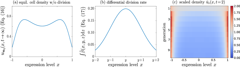
Figure 1: (a) The equilibrium cellular density without division (Eq. (16)). (b) A differential birth rate $\int\tilde{\beta}_{i,j}(X_{i,j},Y,Z)\textrm{d}Z$ using the form given in Eq. (17). (c) Using the differential birth rate in (b) and Eq. (16) for normalization, we plot the associated cellular density $\bar{u}_{i}(x,t=2)$ (Eq. (18)) across different generations. The differentiation process prevents the population from reaching an equilibrium ($i\geq 2$) even when the death rate and division rate are $x$-independent. However, as time increases for a certain generation (such as $i=1$) in which no cell has entered, the structured population in that generation gradually returns to equilibrium.

If the coefficients $g,\sigma,\beta,\tilde{\beta}$ depend only on the cellular internal state $X$ and time $t$ and not on the cells’ generation, we can define

$$\hat{\rho}_{n}(\vec{X}_{n},t)\coloneqq\sum_{\sum{n_{i}}=n}\frac{1}{n!}\sum_{\pi}p_{\bm{n}}(\pi(\bm{X}_{\bm{n}}),t).$$ (19)

where $p_{\bm{n}}$ is defined in Eq. (7) and the summation over $\pi$ is over all possible rearrangements of $\bm{X}_{n}$ (defined in Table 1) of a generation-resolved cell population $\bm{n}$ such that the union of states of all cells in all generations is $\vec{X}_{n}$ (i.e., if we pad $\bm{X}_{\bm{n}}$ into one vector $(X_{1,1},X_{1,2},...,X_{k,n_{k}})$, then such a vector is a rearrangement of $\vec{X}_{n}$, the vector of attributes of all $n$ cells as defined in Table 1).

It can be shown that the differential equation satisfied by $\hat{\rho}_{n}$ is

$$\frac{\partial\hat{\rho}_{n}}{\partial t}+\sum_{j=1}^{n}\frac{\partial(g\hat{\rho}_{n})}{\partial X_{j}}= \mfrac{1}{2}\sum_{j=1}^{n}\frac{\partial^{2}(\sigma^{2}\hat{\rho}_{n})}{(\partial X_{j})^{2}}-\sum_{j=1}^{n}\big{(}\beta(X_{j})+\mu(X_{j})\big{)}\hat{\rho}_{n}$$ (20)

$$+\frac{1}{n}\sum_{j_{1}\neq j_{2}}\!\medint\int\tilde{\beta}(Y,X_{j_{1}},X_{j_{2}})\hat{\rho}_{n-1}(\vec{X}_{n_{\text{b}}}^{{j_{1},j_{2}}},t)\textrm{d}{Y}+(n+1)\int\mu(Y)\hat{\rho}_{n+1}(\vec{X}_{n_{\text{d}}},t)\,\textrm{d}{Y},$$

where $\vec{X}_{n_{\text{b}}}^{j_{1},j_{2}}$ is the pre-division cell states that are different from $\vec{X}_{n}$ in that it does not have contain the $X_{j_{1}},X_{j_{2}}$ terms but has an extra $Y$ at the end; $\vec{X}_{n_{\text{d}}}$ is the pre-death cell states that is different from $\vec{X}$ in that it has an extra $Y$ component. In this case, we can define the generation-independent marginalized cell density

$$u_{n}(\vec{X}_{n},t)\coloneqq\sum_{m\geq n}(m)_{n}\int\hat{\rho}_{m}(\vec{X}_{m},t)\textrm{d}\vec{X}_{m}\backslash\vec{X}_{n}$$ (21)

which satisfies

$$\frac{\partial u_{n}(\vec{X}_{n},t)}{\partial t}+\sum_{j=1}^{n}\frac{\partial(gu_{n})}{\partial X_{j}}= \mfrac{1}{2}\sum_{j=1}^{n}\frac{\partial^{2}(\sigma^{2}u_{n})}{(\partial X_{j})^{2}}-\sum_{j=1}^{n}\big{(}\beta(X_{j})+\mu(X_{j})\big{)}u_{n}$$ (22)

$$+\sum_{j_{1}\neq j_{2}}\int\tilde{\beta}(Y,X_{j_{1}},X_{j_{2}})u_{n-1}(\vec{X}_{n_{\text{b}}}^{{j_{1},j_{2}}},t)\,\textrm{d}{Y}$$

$$+\sum_{j=1}^{n}\int\Big{(}\tilde{\beta}(Y,X_{j},Z)+\tilde{\beta}(Y,Z,X_{j})\Big{)}u_{n}(\vec{X}_{{n}_{{\text{b}}}}^{{{j}}},t)\,\textrm{d}Y\textrm{d}Z.$$

Here, $\vec{X}^{j}_{n_{\text{b}}}$ is different from $\vec{X}_{n}$ in that $X_{j}$ is deleted, but an extra variable $Y$ is added as the last component. If we take $n=1$, we can obtain a closed-form PDE for describing the cell density w.r.t. the scalar state variable $X$

$$\frac{\partial u_{1}(X,t)}{\partial t}+\frac{\partial(gu_{1})}{\partial X}=\mfrac{1}{2}\frac{\partial^{2}(\sigma_{j}^{2}u_{1})}{(\partial X)^{2}}-\big{(}\beta(X)+\mu(X)\big{)}u_{1}+\int\big{(}\tilde{\beta}(Y,X,Z)+\tilde{\beta}(Y,Z,X)\big{)}u_{1}(Y,t)\,\textrm{d}Y\textrm{d}Z.$$ (23)

Eq. (23) is equivalent to the cell sizer model, or a timer-sizer model of cell division [10] after marginalizing over the cells’ ages. As an implementation of this model, one can numerically solve Eq. (22) or (23) using different inferred single-cell-level gene expression dynamics as candidates for $g$ [29].

III.2 Evolution of cell numbers

In the simplest case where all model parameters are constants, we can marginalize over all cell state variables to obtain total cell populations. More specifically, if we define the generation vector $\bm{\bm{i}}\coloneqq(i_{1},...,i_{k}),0<i_{1}<...<i_{k}$ and the associated orders of moments $\bm{\bm{\ell}}\coloneqq(\ell_{1},...,\ell_{k}),\ell_{s}>0$, then we can track the expectation of the product of different orders of the number of cells in different generations

$$\mathds{E}\Big{[}\prod_{s=1}^{k}n_{i_{s}}^{\ell_{s}}\Big{]}\coloneqq\sum_{\bm{n}}\prod_{s=1}^{k}n_{i_{s}}^{\ell_{s}}\int\rho_{\bm{n}}({\bm{X}_{\bm{n}}},t)\,\textrm{d}{\bm{X}_{\bm{n}}}.$$ (24)

The differential equation satisfied by $\mathds{E}\big{[}\prod_{i=1}^{k}n_{i}^{\ell_{i}}\big{]}$ can be shown to be

$$\frac{\textrm{d}\mathds{E}\big{[}\prod_{s=1}^{k}n_{i_{s}}^{\ell_{s}}\big{]}}{\textrm{d}t}= \sum_{r=1,i_{r}>1}^{k}\beta_{i_{r}-1}\Big{(}\mathds{E}\big{[}\prod_{s=1}^{k}(n_{i_{s}}-\delta_{i_{r}-1,i_{s}}+2\delta_{i_{r},i_{s}})^{\ell_{s}}n_{i_{r}-1}\big{]}-\mathds{E}\big{[}\prod_{s=1}^{k}n_{i_{s}}^{\ell_{s}}n_{i_{r}-1}\big{]}\Big{)}$$ (25)

$$+\sum_{r=1}^{k}\beta_{i_{r}}\Big{(}\mathds{E}\big{[}\prod_{s=1}^{k}(n_{i_{s}}-\delta_{i_{r},i_{s}}+2\delta_{i_{r}+1,i_{s}})^{\ell_{s}}n_{i_{r}}\big{]}-\mathds{E}\big{[}\prod_{s=1}^{k}n_{i_{s}}^{\ell_{s}}n_{i_{r}}\big{]}\Big{)}$$

$$-\sum_{r=1}^{k-1}\beta_{i_{r}}\bigg{(}\delta_{i_{r+1}-i_{r},1}\Big{(}\mathds{E}\big{[}\prod_{s=1}^{k}(n_{i_{s}}-\delta_{i_{r},i_{s}}+2\delta_{i_{r}+1,i_{s}})^{\ell_{s}}n_{i_{r}}\big{]}-\mathds{E}\big{[}\prod_{s=1}^{k}n_{i_{s}}^{\ell_{s}}n_{i_{r}}\big{]}\Big{)}\bigg{)}$$

$$-\sum_{r=1}^{\infty}\mu_{i_{r}}\Big{(}\mathds{E}\big{[}\prod_{s=1}^{k}n_{i_{s}}^{\ell_{s}}n_{i_{r}}\big{]}-\mathds{E}\big{[}\prod_{s=1}^{k}(n_{i_{s}}-\delta_{i_{s},i_{r}})^{\ell_{s}}n_{i_{r}}\big{]}\Big{)}.$$

where $\delta_{i_{r},i_{s}}=1$ if $i_{r}=i_{s}$ and $\delta_{i_{r},i_{s}}=0$ otherwise is the Kronecker $\delta$-function. Note that if $\bm{i}=(i)$ is one-dimensional, and $\bm{\ell}=(1)$, then Eq. (25) reduces to the evolution of the average cell number in the $i^{\text{th}}$ generation

$$\frac{\textrm{d}\mathds{E}[n_{i}]}{\textrm{d}t}=2\beta_{i-1}\mathds{E}[n_{i-1}]-\beta_{i}\mathds{E}[n_{i}]-\mu_{i}\mathds{E}[n_{i}].$$ (26)

Finally, we can consider another special simplifying case where

$$P(\bm{n},t)\coloneqq\int\!\rho_{\bm{n}}(\bm{X}_{\bm{n}},t)\textrm{d}{\bm{X}_{\bm{n}}}$$ (27)

is the probability that the population contains $\{n_{1},n_{2},\ldots,n_{k}$ cells in generations $1,\ldots,k$, respectively, regardless of the individual’s values of $X$. It turns out that $P(\bm{n})$ satisfies the series of interdependent master equations

$$\frac{\textrm{d}P(\bm{n},t)}{\textrm{d}t}=\sum_{i=1}^{k-1}\beta_{i-1}(n_{i-1}+1)P(\bm{n}_{\text{b},i},t)-\sum_{i=1}^{k}\big{(}\beta_{i}+\mu_{i}\big{)}n_{i}P(\bm{n},t)+\sum_{i=1}^{\infty}\mu_{i}(n_{i}+1)P(\bm{n}_{\text{d},i},t).$$ (28)

when the division rates and the birth rates are constants within the same generation, i.e., $\mu_{i,j}\equiv\mu_{i},\beta_{i,j}\equiv\beta_{i},\beta_{0}\coloneqq 0$. Eq. (28) is a multigenerational birth-death master equation for the number of individuals in each generation $i$ which carries the same structure as birth-death processes for cells grouped by different attributes other than generation [30]. Note that generating new members of a successive generation arises only from birth, while death only decreases the numbers within a generation.

III.3 Evolution of “biomass”

Another quantity of specific interest is the biomass (e.g., the total amount of protein or mRNA within a subpopulation). For example, the total mass within cells of the $i^{\rm th}$ generation can be defined as $X_{i}\equiv\sum_{j=1}^{n_{i}}X_{i,j}$ and its expectation evaluated from

$$\mathds{E}\big{[}X_{i}(t)\big{]}=\sum_{\bm{n}}\int\Big{(}\sum_{j=1}^{n_{i}}X_{i,j}\Big{)}\rho_{\bm{n}}(\bm{X}_{\bm{n}},t)\textrm{d}\bm{X}_{\bm{n}}$$ (29)

where $\rho_{\bm{n}}(\bm{X}_{\bm{n}},t)$ is defined in Eq. (10).

In general, the differential equation satisfied by $X_{i}(t)$ involves higher moment quantities; thus, the model is not closed. However, given certain constraints on the parameters, the dynamics for $X_{i}(t)$ can be closed, and a solution can be explicitly computed (analytically, or numerically). For example, if $\beta_{i}(X_{i,j})\coloneqq\beta_{i},\mu_{i}(X_{i,j})\coloneqq\mu_{i}$ are constants, $g_{i}(X_{i,j})\coloneqq g_{i}X_{i,j}$ is linear, and the quantity $X$ is conserved across cell division (that is, if the mother cell carries the state variable $X$ and the two daughter cells have are in states $Y_{1}$ and $Y_{2}$, then $Y_{1}+Y_{2}=X$), then

$$\frac{\textrm{d}\mathds{E}[X_{i}(t)]}{\textrm{d}t}=\big{(}g_{i}-\mu_{i}-\beta_{i}\big{)}\mathds{E}\big{[}X_{i}(t)\big{]}+\beta_{i-1}\mathds{E}\big{[}X_{i-1}(t)\big{]}.$$ (30)

Furthermore, if the growth rate and division rate are independent of the generation number $i$, we can define expectations over any moment of the total biomass summed over cells of all generations as

$$\mathds{E}\big{[}X^{q}(t)\big{]}=\sum_{\bm{n}}\int\Big{(}\sum_{i=1}^{k}\sum_{j=1}^{n_{i}}X_{i,j}\Big{)}^{q}\rho_{\bm{n}}(\bm{X}_{\bm{n}},t)\,\textrm{d}{\bm{X}_{\bm{n}}},\quad q>1.$$ (31)

Specifically, if $\mu$ is a constant and $g(X)=g_{0}X$ (and $X$ is conserved across cell division), the differential equations satisfied by the first and second moments of the total biomass $X(t)$ and $X^{2}(t)$ are

$$\frac{\textrm{d}\mathds{E}[X(t)]}{\textrm{d}t} =\big{(}g_{0}-\mu\big{)}\int xu_{1}(x,t)\textrm{d}x\equiv\big{(}g_{0}-\mu\big{)}\mathds{E}\big{[}X(t)\big{]},$$ (32)

$$\frac{\textrm{d}\mathds{E}\big{[}X^{2}(t)\big{]}}{\textrm{d}t} =\big{(}g_{0}-2\mu\big{)}\mathds{E}\big{[}X^{2}(t)\big{]}+\sigma^{2}\mathds{E}\big{[}X(t)\big{]}+\mu\int x^{2}u_{1}(x,t)\textrm{d}x.$$

Only the equation for the mean total biomass $\mathds{E}[X(t)]$ is closed. Its second moment depends on averages over $u_{1}(x,t)$ requiring the solution to Eq. (23). General cases for the equations satisfied by $\mathds{E}\big{[}X^{q}(t)\big{]}$ for arbitrary $q\in\mathbb{N}^{+}$ are discussed in Appendix B.

III.4 Tracking dead cells

Thusfar, we have assumed that the “biomass” $X$ originates from live cells. Once cells die, they are no longer counted in the population and the biomass $X$ associated with them is no longer included. However, experimentally, the protein and/or mRNA extracted from a solution of cells may come from both living and dead cells (at the time of extraction). To describe these types of measurements, we keep track of cells that have died and assign them to the $0^{\text{th}}$ generation $g_{0}=\beta_{0}=0$. We denote their states by $\bm{X}_{0}\coloneqq(X_{0,1},...,X_{0,n_{0}})$. We then define $\tilde{p}_{\bm{n}}(\bm{X}_{\bm{n}},t|\bm{X}(0)_{\bm{n}(0)},0)$ to include the zero-generation (cells that have died) population. Using arguments similar to those in Proposition 2 we can show that under certain conditions $\tilde{p}_{\bm{n}}$ satisfies the differential equation

$$\frac{\partial\tilde{p}_{\bm{n}}}{\partial t}+\sum_{i=1}^{k}\sum_{j=1}^{n_{i}}\frac{\partial(g_{i,j}\tilde{p}_{\bm{n}})}{\partial X_{i,j}}= \mfrac{1}{2}\sum_{i=1}^{k}\sum_{j=1}^{n_{i}}\frac{\partial^{2}(\sigma^{2}_{i,j}\tilde{p}_{\bm{n}})}{(\partial X_{i,j})^{2}}-\sum_{i=1}^{k}\sum_{j=1}^{n_{i}}\big{(}\beta_{i,j}+\mu_{i,j}\big{)}\tilde{p}_{\bm{n}}$$ (33)

$$\,\,+\sum_{i=1}^{k-1}\sum_{j=1}^{n_{i-1}+1}\!nt\tilde{\beta}_{i,j}(Y,X_{i+1,n_{i+1}-1},X_{i+1,n_{i+1}})\tilde{p}_{\bm{n}_{\text{b},i}}(\bm{X}_{\bm{n}_{\text{b},i}^{j}}\!t|\bm{X}(0)_{\bm{n}(0)},0)\,\textrm{d}{Y}$$

$$\,\,+\sum_{i=1}^{\infty}\sum_{j=1}^{n_{i}+1}\mu(X_{0,n_{0}})\tilde{p}_{\bm{n}_{\tilde{\text{d}},i}}(\bm{X}_{\bm{n}_{\tilde{\text{d}},i}}^{j}\!t|\bm{X}(0)_{\bm{n}(0)},0)$$

where $\bm{n}_{\tilde{\text{d}},i}$ differs from in that its $0^{\text{th}}$ component is $n_{0}-1$ but its $i^{\text{th}}$ component is $n_{i}+1$, and $\bm{X}_{\bm{n}_{\tilde{\text{d}},i}}^{j}$ differs from $\bm{X}_{\bm{n}}$ in that the internal states of the $0^{\text{th}}$ generation (dead cells) are $(X_{0,1},...,X_{0,n_{0}-1})$ and the internal states of the $i^{\text{th}}$ generation are $(X_{i,1},...,X_{i,j-1},X_{0,n_{0}},X_{i,j},...,X_{i,n_{i}})$ ($X_{0,n_{0}}$ is in the $j^{\text{th}}$ component). Similarly, we can define the unconditional probability density function $\tilde{p}_{\bm{n}}^{*}(\bm{X}_{\bm{n}},t)$ as defined in Eq. (7) as well as the symmetrized probability density function

$$\tilde{\rho}_{\bm{n}}(\bm{X}_{\bm{n}},t)\coloneqq\prod_{i=0}^{k}\frac{1}{n_{i}!}\sum_{\pi}\tilde{p}_{\bm{n}}^{*}(\pi(\bm{X}_{\bm{n}}),t).$$ (34)

The PDE satisfied by $\tilde{\rho}_{\bm{n}}$ is

$$\frac{\partial\tilde{\rho}_{\bm{n}}}{\partial t}+\sum_{i=1}^{k}\sum_{j=1}^{n_{i}}\frac{\partial(g_{i,j}\tilde{\rho}_{\bm{n}})}{\partial X_{i,j}}= \mfrac{1}{2}\sum_{i=1}^{k}\sum_{j=1}^{n_{i}}\frac{\partial^{2}(\sigma_{i,j}^{2}\tilde{\rho}_{\bm{n}})}{(\partial X_{i,j})^{2}}-\sum_{i=1}^{k}\sum_{j=1}^{n_{i}}\big{(}\beta_{i,j}+\mu_{i,j}\big{)}\tilde{\rho}_{\bm{n}}$$ (35)

$$\,\,+\sum_{i=1}^{k-1}\frac{n_{i}+1}{n_{i+1}(n_{i+1}-1)}\sum_{j_{1}\neq j_{2}}\!\medint\int\!\tilde{\beta}_{i,j}(Y,X_{i+1,j_{1}},X_{i+1,j_{2}})\tilde{\rho}_{\bm{n}_{\text{b},i}}(\bm{X}_{\bm{n}_{\text{b},i}}^{{j_{1},j_{2}}},t)\,\textrm{d}{Y}$$

$$\,\,+\frac{1}{n_{0}}\sum_{i=1}^{\infty}(n_{i}+1)\sum_{j=1}^{n_{0}}\mu_{i,j}(X_{0,j})\rho_{\bm{n}_{\tilde{\text{d}},i}}(\bm{X}_{\bm{n}_{\tilde{\text{d}},i}}^{j},t).$$

The expectation of the total biomass $X_{0}\equiv\sum_{j=1}^{n_{0}}X_{0,j}$ associated with dead cells can be found from

$$\mathds{E}\big{[}X_{0}(t)\big{]}\equiv\sum_{\bm{n}}\int\big{(}\sum_{j=1}^{n_{0}}X_{0,j}\big{)}\tilde{\rho}_{\bm{n}}(\bm{X}_{\bm{n}},t)\,\textrm{d}{\bm{X}_{\bm{n}}}.$$ (36)

If the death rates $\mu_{i}$ of cells are equal and constant within each generation $i$, then $\mathds{E}\big{[}X_{0}(t)\big{]}$ satisfies

$$\frac{\textrm{d}\mathds{E}\big{[}X_{0}(t)\big{]}}{\textrm{d}t}=\sum_{i=1}^{\infty}\mu_{i}\mathds{E}\big{[}X_{i}(t)\big{]},$$ (37)

where $\mathds{E}\big{[}X_{i}(t)\big{]}$ is the total expected biomass from cells in the $i^{\text{th}}$ generation, as defined in Eq. (29).

We can also define second moments involving the biomass from dead cells

$$\mathds{E}\big{[}X_{0}^{2}(t)\big{]}=\sum_{\bm{n}}\int\big{(}\sum_{j=1}^{n_{0}}X_{0,j}\big{)}^{2}\tilde{\rho}_{\bm{n}}(\bm{X}_{\bm{n}},t)\,\textrm{d}{\bm{X}_{\bm{n}}}$$ (38)

and

$$\mathds{E}\big{[}X_{0}(t)X(t)\big{]}=\sum_{\bm{n}}\int\Big{(}\sum_{i=1}^{k}\sum_{j=1}^{n_{i}}X_{i,j}\Big{)}\Big{(}\sum_{\ell=1}^{n_{0}}X_{0,\ell}\Big{)}\tilde{\rho}_{\bm{n}}(\bm{X}_{\bm{n}},t)\,\textrm{d}{\bm{X}_{\bm{n}}}.$$ (39)

If we assume that the death rate is a constant $\mu$ for all cells, the growth rate $g(X)=g_{0}X$, and the state variable $X$ is conserved at division, we can derive the differential equations

$$\frac{\textrm{d}\mathds{E}\big{[}X_{0}^{2}(t)\big{]}}{\textrm{d}t}=2\mu\mathds{E}\big{[}X_{0}(t)X(t)\big{]}+\mu\sum_{\bm{n}}\int\Big{(}\sum_{i=1}^{k}\sum_{j=1}^{n_{i}}X_{i,j}^{2}\Big{)}\tilde{\rho}_{\bm{n}}(\bm{X}_{\bm{n}},t)\,\textrm{d}\bm{X}_{\bm{n}}$$ (40)

$$\frac{\textrm{d}\mathds{E}\big{[}X_{0}(t)X(t)\big{]}}{\textrm{d}t}=(g_{0}-\mu)\mathds{E}\big{[}X_{0}(t)X(t)\big{]}+\mu\mathds{E}\big{[}X^{2}(t)\big{]}-\mu\sum_{\bm{n}}\int\Big{(}\sum_{i=1}^{k}\sum_{j=1}^{n_{i}}X_{i,j}^{2}\Big{)}\tilde{\rho}_{\bm{n}}(\bm{X}_{\bm{n}},t)\,\textrm{d}{\bm{X}_{\bm{n}}}.$$ (41)

Higher moments of $X_{0},X$ can also be evaluated, which we do not include for brevity.

III.5 Correlations and interactions

Although examples so far have involved simple forms of $g,\sigma,\beta,\mu$ that depend only on the state of of the cell being tracked, these rates can depend on the states of other cells in the population. These more complex dependences prevent closure of the PDEs and signal more complex correlations, or “interactions.” Simple interactions can be incorporated in the “mean-field” limit if we consider the parameters $g,\sigma,\beta,\mu$ to be functions of only averaged macroscopic quantities such as $X(t)$.

As an intuitive example, if we allow the death rate of the $j^{\text{th}}$ cell in the $i^{\text{th}}$ generation to also depend on the total “biomass” from all living cells, $\mu_{i,j}=\mu_{i,j}(X_{i,j},\sum_{i}\sum_{j=1}^{n_{i}}X_{i,j})$. Using this form of death rate leads to a symmetric population density $\rho_{\bm{n}}(\{X\}_{\bm{n}}$ that satisfies

$$\frac{\partial\rho_{\bm{n}}}{\partial t}+\sum_{i=1}^{k}\sum_{j=1}^{n_{i}}\frac{\partial(g_{i}\rho_{\bm{n}})}{\partial X_{i,j}}= \mfrac{1}{2}\sum_{i=1}^{k}\sum_{j=1}^{n_{i}}\frac{\partial^{2}(\sigma_{i,j}\rho_{\bm{n}})}{(\partial X_{i,j})^{2}}-\sum_{i=1}^{k}\sum_{j=1}^{n_{i}}\Big{(}\beta_{i,j}(X_{i,j})+\mu_{i,j}\big{(}X_{i,j},{\displaystyle\medop\sum_{\ell=1}^{k}\medop\sum_{m=1}^{n_{\ell}}X_{\ell,m}}\big{)}\Big{)}\rho_{\bm{n}}$$ (42)

$$\quad+\sum_{i=1}^{k-1}\frac{n_{i}+1}{n_{i+1}(n_{i+1}-1)}\!\sum_{1\leq j_{1}\neq j_{2}\leq n_{i+1}}\!\!\!\!\!int\int\tilde{\beta}_{i}(Y,X_{i+1,j_{1}},X_{i+1,j_{2}})\rho_{\bm{n}_{\text{b},i}}(\bm{X}_{\bm{n}_{\text{b},i}}^{{j_{1},j_{2}}},t)\,\textrm{d}{Y}$$

$$\quad+\sum_{i=1}^{\infty}\sum_{j=1}^{n_{i}+1}\int\mu_{i,j}\big{(}Y,\,{\displaystyle\medop\sum_{\ell=1}^{k}\medop\sum_{m=1}^{n_{\ell}}X_{\ell,m}+Y}\big{)}\rho_{\bm{n}_{\text{d}}}(\bm{X}_{\bm{n}_{\text{d},i}}^{{j}},t)\textrm{d}{Y}.$$

Due to the dependencies on the mean-field term $\sum_{i=1}^{k}\sum_{j=1}^{n_{i}}X_{i,j}$, we cannot obtain a closed-form equation for macroscopic quantities such as the cellular density $u_{1}(X_{1},t)$ defined in Eq. (23). However, if the approximation $\sum_{i=1}^{k}\sum_{j=1}^{n_{i}}X_{i,j}\approx\sum_{i=1}^{k}\sum_{j=1}^{n_{i}}X_{i,j}+Y\approx\mathds{E}[X(t)]$ can be made, with $\mathds{E}[X(t)]$ defined in Eq. (29), an approximate PDE for $u_{1}(X,t)$ defined in Eq. (21) can be motivated:

$$\frac{\partial u_{1}(X_{1},t)}{\partial t}+\frac{\partial(gu_{1})}{\partial X_{1}}= \mfrac{1}{2}\frac{\partial^{2}(\sigma_{j}^{2}u_{1})}{(\partial X_{1})^{2}}-\Big{(}\beta(X_{1})+\mu\big{(}X_{1},\medint\int Yu_{1}(Y,t)\text{d}Y\big{)}\Big{)}u_{1}(X,t)$$ (43)

$$\qquad\qquad\qquad+\!\int\!\Big{(}\tilde{\beta}(Y,X_{1},Z)+\tilde{\beta}(Y,Z,X_{1})\Big{)}u_{1}(Y,t)\,\textrm{d}Y\textrm{d}Z.$$

Eq. (43) is nonlinear because the mean-field term depends on $\int xu_{1}(x,t)\text{d}x$. Similarly, if other coefficients depend on mean-field quantities or some specific interaction terms among cells exist, then by making assumptions and marginalization, it might still be possible to find self-consistent integrodifferential equations for macroscopic quantities of interest. For example, death rates that depend on the values of $X$ of two different cells have been shown to generate a nonlinear interaction term in kinetic derivations of single-species predator-prey type models [31].

IV Summary and Conclusions

In this work, we used the forward-type Feynman-Kac formula and Markov jump process to formulate a kinetic theory for describing the cellular population density of a generation-resolved cellular population with fluctuating rates of changing internal states as well as random division times. Such a general kinetic theory not only tracks each cell’s continuous-valued state attribute such as its volume, protein or mRNA abundance, but also its generation (i.e., how many times its ancestors have divided). In general, our kinetic theory framework can apply to any collection of particles that experience demographic noise from birth-death processes as well as noise in specific individual-level attributes.

A number of new results were presented. The underlying kinetic theory describing the intra-generation-symmetrized cell populations is given by Eq. (10) (or Eq. (12) for a vector of attributes). We find that this fully resolved, high-dimensional probability density can be marginalized in to different directions. First, one can sum over moments of the discrete populations/subpopulations to find the dynamics of a generalized cell population density $u_{\bm{n}}(\bm{X}_{\bm{n}},t)$ (Eq. (13)), which is found to obey Eq. (14) when generations are tracked, and Eq. (23) in the generation-independent case. Further marginalizing over all cell attributes $\bm{X}_{\bm{n}}$ allows one to derive simpler equations for useful quantities such as the expected total number of cells in each generation (Eq. (26)) and the generation structure of the total population (Eq. (28)).

Alternatively, the full probability densities can be used to define moments of mean-field quantities such as total gene expression levels or biomass $X$ across the entire population. These are derived in Eqs. (30) and (32), which depend on integrals over the single-particle number density $u_{1}(x,t)$. We also show how the biomass $X_{0}$ from dead calls can also be tracked, as is often the case in experiments. Expressions for the lowest moments are given in Eqs. (37), (40), and (41). Our results are tabulated below:

Quantity	Meaning	Equation
$u_{\bm{n}}(\bm{X}_{\bm{n}},t)$	partially marginalized cell population density of any order	Eq. (14). Closed set of PDEs for noninteracting systems
$u_{n}(\vec{X}_{n},t)$	generation-independent cell population density (may include intercellular dependence)	Eqs. (21) and (22)
$\mathbb{E}[\bm{n}(t)]$	expectation of moments of total cell number	Eqs. (24), (25), and (26)
$P(\bm{n},t)$	probability of $\bm{n}=\{n_{i}\}$ in each generation $i$	Eqs. (27) and (28)
$\mathbb{E}[X^{q}(t)]$	expectation of moments of total biomass or expression levels	Eqs. (31), (32), and (23)
$\mathbb{E}[X_{0}^{p}(t)X^{q}(t)],\,p+q\leq 2$	mean and variance of biomass from dead cells	Eqs. (37),(38),(39), (40), (41), and (35)

Table 2: Summary of our main results. Functions describing cell numbers and overall attributes are listed, along with the equation numbers of their mathematical definitions and dynamical equations.

Finally, we discussed cell-cell “interactions” that manifest themselves through birth or death rates that depend on the attribute $X_{i,j}$ of multiple cells. Such forms of the birth and death rate precludes full marginalization, leading to higher order correlation terms for which an approximation must be imposed to close the equations. We show how a death rate that also depends on the total biomass results in the implicitly nonlinear (in $u_{1}(x,t)$) PDE given in  (43).

Note that the PDEs for marginalized densities $u_{\bm{n}}(\bm{X}_{\bm{n}},t)$ can be solved numerically using newly developed adaptive spectral methods suited for unbounded domains [32, 33, 34] and provide an “Eulerian” representation of the structured population. Our kinetic theory/PDE framework does not directly track the structure of populations along lineages of cells (a more “Lagrangian” picture) but connecting our Eulerian representation with representations that delineate cell lineages would be useful area of future analysis.

Other directions for future analysis include developing tractable models of interactions that arise through complex dependences of birth and death rates on $\bm{X}_{\bm{n}}$. The equations we derived can also inform inverse-type problems by serving as constraints for neural network-based machine learning approaches for inferring model parameters (such as interacting birth and death rates) from data [35]. Structured populations that vary spatially also arise in many applications [36, 37, 38]. For models in which convection and diffusion depend on expression levels, the dynamics of $\bm{X}_{\bm{n}}$ can be modeled as being coupled to transport.

Data Availability The datasets generated during and/or analysed during the current study are available from the corresponding author on reasonable request. Declarations Conflict of Interest The authors declare that they have no known competing financial interests or personal relationships that could have appeared to influence the work reported in this paper.

Appendix A Derivation of the differential equation satisfied by the cell population probability density function

To show $p_{\bm{n}}(\bm{X}_{\bm{n}},t|\bm{X}(0)_{\bm{n}(0)},0)$ defined in Eq. (4) satisfies Eq. (6), we require the following two propositions.

Proposition 1.

(Forward-type Feynman-Kac formula) If the coefficients $g_{i,j},\sigma_{i,j},\beta_{i,j},\mu_{i,j}$ are smooth, uniform Lipschitz continuous, and uniformly bounded, then, under certain conditions, the solution to the following PDE

$$\frac{\partial\hat{p}_{\bm{n}}(\bm{X}_{\bm{n}},t|\bm{X}(0)_{\bm{n}(0)},0)}{\partial t}+\!\sum_{i=1}^{k}\sum_{j=1}^{n_{i}}\frac{\partial(g_{i,j}(X_{i,j},t)\hat{p}_{\bm{n}})}{\partial X_{i,j}}= \mfrac{1}{2}\sum_{i=1}^{k}\sum_{j=1}^{n_{i}}\frac{\partial^{2}(\sigma_{i,j}^{2}(X_{i,j},t)\hat{p}_{\bm{n}})}{(\partial X_{i,j})^{2}}$$ (A1)

$$\quad-\sum_{i=1}^{k}\sum_{j=1}^{n_{i}}\!\big{(}\beta_{i,j}(X_{i,j})+\mu_{i,j}(X_{i,j})\big{)}\hat{p}_{\bm{n}}$$

with initial condition $\hat{p}_{\bm{n}}(\bm{X}_{\bm{n}},0)=\delta(\bm{X}(0)_{\bm{n}(0)}-\bm{X}_{\bm{n}})$ if $\bm{n}=\bm{n}(0)$ (and $\hat{p}_{\bm{n}}(\bm{X}(0)_{\bm{n}(0)},0)=0$ if $\bm{n}\neq\bm{n}(0)$), is

$$\hat{p}_{\bm{n}}(\bm{X}_{\bm{n}},t|\bm{X}(0)_{\bm{n}(0)},0)\coloneqq\mathbb{E}\Big{[}\delta(\bm{X}(t)_{\bm{n}(t)}-\bm{X}_{\bm{n}})S\big{(}t;\bm{X}(t)_{\bm{n}(t)}\big{)}\Big{|}\bm{X}(0)_{\bm{n}(0)},0;\bm{n}(0\leq s\leq t)=\bm{n}(0)\Big{]}$$ (A2)

where each component in $\bm{X}(t)_{\bm{n}(t)}$ satisfies Eq. (1).

Proposition 1 provides the PDE satisfied by the density function for all cells with states $\bm{X}_{\bm{n}}$ in the absence of division and death. The proof of Proposition 1 and the associated specific technical assumptions are given in section A.1 below.

When cell division or death occurs, the total number of cells changes according to a Markov jump process. Thus, we need the following proposition to derive the differential equation satisfied by the conditional probability density function $p_{\bm{n}}(\bm{X}_{\bm{n}},t|\bm{X}(0)_{\bm{n}(0)},0)$ defined in Eq. (4).

Proposition 2.

(Markov jump process) Given the initial condition $\bm{n}(0)$ with states $\bm{X}(0)_{\bm{n}(0)}$ at $t=0$ and a target state at time $t$ with $\bm{n}$ cells and their internal states $\bm{X}_{\bm{n}}$, we start with the conditions

$$p^{0}_{\bm{n}}(\bm{X}_{\bm{n}},t|\bm{X}(0)_{\bm{n}(0)},0)\coloneqq 0,$$ (A3)

$$p^{1}_{\bm{n}}(\bm{X}_{\bm{n}},t|\bm{X}(0)_{\bm{n}(0)},0)\coloneqq \hat{p}_{\bm{n}}(\bm{X}_{\bm{n}},t|\bm{X}(0)_{\bm{n}(0)},0),$$

and recursively define

$$p_{\bm{n}}^{m+1}(\bm{X}_{\bm{n}},t|\bm{X}(0)_{\bm{n}(0)},0)\coloneqq \hat{p}_{\bm{n}}(\bm{X}_{\bm{n}},t|\bm{X}(0)_{\bm{n}(0)},0)$$ (A4)

$$+\int_{0}^{t}\mathbb{E}\Big{[}S\big{(}\tau;\bm{X}(\tau)_{\bm{n}(\tau)}\big{)}J^{m}\big{(}t,\tau;\bm{X}_{\bm{n}},\bm{n}(0)\big{)}\Big{|}\bm{X}(0)_{\bm{n}(0)},0;\bm{n}(0<s<\tau)=\bm{n}(0)\Big{]}\textrm{d}{\tau},$$

where the birth-death probability flux is defined by

$$J^{m}\big{(}t,\tau;\bm{X}_{\bm{n}},\bm{n}(0)\big{)}\coloneqq \sum_{i=1}^{k(0)}\sum_{j=1}^{n_{i}(0)}\Big{[}\tilde{\beta}_{i,j}\big{(}X_{i,j}(\tau),X_{1}(\tau),X_{2}(\tau)\big{)}p_{\bm{n}}^{m}(\bm{X}_{\bm{n}},t-\tau|\bm{X}(\tau)_{\bm{n}(0)_{\text{b},-i}}^{-j},0)$$ (A5)

$$\hskip 102.43008pt+\mu_{i,j}\big{(}X_{i,j}(\tau)\big{)}p_{\bm{n}}^{m}(\bm{X}_{\bm{n}},t-\tau|\bm{X}(\tau)_{\bm{n}(0)_{\text{d},-i}}^{-j},0)\Big{]}.$$

Then, $p_{\bm{n}}^{m+1}$ satisfies

$$\frac{\partial p_{\bm{n}}^{m+1}}{\partial t}+\sum_{i=1}^{k}\sum_{j=1}^{n_{i}}\frac{\partial(g_{i,j}p^{m+1}_{\bm{n}})}{\partial X_{i,j}}= \mfrac{1}{2}\sum_{i=1}^{k}\sum_{j=1}^{n_{i}}\frac{\partial^{2}(\sigma_{i,j}^{2}p^{m+1}_{\bm{n}})}{(\partial X_{i,j})^{2}}-\sum_{i=1}^{k}\sum_{j=1}^{n_{i}}\big{(}\beta_{i,j}(X_{i,j})+\mu_{i,j}(X_{i,j})\big{)}p^{m+1}_{\bm{n}}$$ (A6)

$$+\sum_{i=1}^{k-1}\sum_{j=1}^{n^{\text{b}}_{i-1}}\!\int\tilde{\beta}(Y,X_{i+1,n_{i+1}-1},X_{i+1,n_{i+1}})p^{m}_{\bm{n}_{\text{b},i}}(\bm{X}^{j}_{\bm{n}_{\text{b},i}},t\,|\,\bm{X}(0)_{\bm{n}(0)},0)\textrm{d}{Y}$$

$$+\sum_{i=1}^{\infty}\sum_{j=1}^{n_{i}^{\text{d}}}\int\!\mu({\textbf{}Y})p^{m}_{\bm{n}_{\text{d},i}}(\bm{X}^{j}_{\bm{n}_{\text{d},i}},t\,|\,\bm{X}(0)_{\bm{n}(0)},0)\textrm{d}{{\textbf{}Y}}.$$

Furthermore, $p_{\bm{n}}^{m}$ is non-decreasing in $m$.

The proof of Proposition 2 will be given in section A.2 below. Intuitively, $m$ in Eq. (A4) is the maximal number of birth or death events allowed within the cell population. Since $p_{\bm{n}}^{m}$ is increasing in $m$, there exists a $p^{*}$ such that $p^{m}\rightarrow p^{*}$ a.s. for all $\bm{X}(0)_{\bm{n}(0)}$ and $\bm{X}_{\bm{n}}$. After integrating over $\bm{X}_{\bm{n}}$ and summing over all $\bm{n}$ on both sides of Eq. (A4) and assuming

$$\sum_{{\bm{n}}}\int p_{\bm{n}}^{m-1}(\bm{X}_{\bm{n}},t|\bm{X}(0)_{\bm{n}(0)},0)\,\textrm{d}{\bm{X}_{\bm{n}}}\leq 1$$ (A7)

for $m\in\mathbb{N}$ and any initial condition $\bm{X}(0)_{\bm{n}(0)}$, we have $\sum_{{\bm{n}}}\int p_{\bm{n}}^{m}(\bm{X}_{\bm{n}},t\,|\,\bm{X}(0)_{\bm{n}(0)},0)\textrm{d}{\bm{X}_{\bm{n}}}\leq F^{m}(t;\bm{X}(0)_{\bm{n}(0)},0)$ where

$$F^{m}(t;\bm{X}(0)_{\bm{n}(0)},0)\coloneqq \!\int\hat{p}_{\bm{n}(0)}(\bm{X}_{\bm{n}(0)},t\,|\,\bm{X}(0)_{\bm{n}(0)},0)\textrm{d}\bm{X}_{\bm{n}(0)}$$ (A8)

$$+\int_{0}^{t}\mathbb{E}\Big{[}S\big{(}\tau;\bm{X}(\tau)_{\bm{n}(\tau)}\big{)}\sum_{i=1}^{k(0)}\sum_{j=1}^{n_{i}(0)}\big{(}\beta(X_{i,j}(\tau))+\mu(X_{i,j}(\tau)\big{)}\big{|}\bm{X}(0)_{\bm{n}(0)},0;\bm{n}(0<s<\tau)=\bm{n}(0)\Big{]}\,\textrm{d}{\tau}$$

and $S\big{(}\tau;\bm{X}(\tau)_{\bm{n}(\tau)}\big{)}$ is defined in Eq. (5). Taking the derivative of $F^{m}(t;\bm{X}(0)_{\bm{n}(0)},0)$, we find $\textrm{d}F^{m}(t;\bm{X}(0)_{\bm{n}(0)},0)/\textrm{d}t=0$. It is straightforward to verify that $F^{m}(0;\bm{X}(0)_{\bm{n}(0)},0)=1$; therefore, we have $F^{m}(t;\bm{X}(0)_{\bm{n}(0)},0)\equiv 1,\forall t\geq 0$, which indicates that

$$\sum_{\bm{n}}\int p_{\bm{n}}^{m}(\bm{X}_{\bm{n}},t|\bm{X}(0)_{\bm{n}(0)},0)\textrm{d}\bm{X}_{\bm{n}}\leq 1.$$ (A9)

By induction, Eq. (A7) holds true for all $m\in\mathbb{N}^{+}$. Finally, it is easy to show that $p_{\bm{n}}^{m}(\bm{X}(0)_{\bm{n}},t|\bm{X}(0)_{\bm{n}(0)},0)\geq 0$, so by the monotone convergence theorem,

$$\sum_{\bm{n}}\int p_{\bm{n}}^{*}(\bm{X}_{\bm{n}},t|\bm{X}(0)_{\bm{n}(0)},0)\textrm{d}\bm{X}_{\bm{n}}\leq 1,$$ (A10)

which indicates $0\leq p^{*}<\infty$ exists a.e..

If i) the convergence $p^{m}\rightarrow p^{*}$ is uniform and ii) taking the limit w.r.t. $m$ is interchangeable with taking the partial derivatives in Eq. (A6), then $p^{*}$ is the solution to

$$\frac{\partial p_{\bm{n}}^{*}}{\partial t}+\sum_{i=1}^{k}\sum_{j=1}^{n_{i}}\frac{\partial(g_{i,j}p^{*}_{\bm{n}})}{\partial X_{i,j}}= \mfrac{1}{2}\sum_{i=1}^{k}\sum_{j=1}^{n_{i}}\frac{\partial^{2}(\sigma_{i,j}p^{*}_{\bm{n}})}{(\partial X_{i,j})^{2}}-\sum_{i=1}^{k}\sum_{j=1}^{n_{i}}\big{(}\beta(X_{i,j})+\mu(X_{i,j})\big{)}p^{*}_{\bm{n}}$$ (A11)

$$+\sum_{i=1}^{k-1}\sum_{j=1}^{n_{i}+1}\!\int\tilde{\beta}_{i,j}(Y,X_{i+1,n_{i+1}-1},X_{i+1,n_{i+1}})p^{*}_{\bm{n}_{\text{b},i}}(\bm{X}^{j}_{\bm{n}_{\text{b},i}},t|\bm{X}(0)_{\bm{n}(0)},0)\textrm{d}{Y}$$

$$+\sum_{i=1}^{\infty}\sum_{j=1}^{n_{i}+1}\!\int\mu_{i,j}({\textbf{}Y})p^{*}_{\bm{n}_{\text{d},i}}(\bm{X}^{j}_{\bm{n}_{\text{d},i}},t|\bm{X}(0)_{\bm{n}(0)},0)\textrm{d}{{\textbf{}Y}}$$

Since by taking the limit $m\rightarrow\infty$ in Eq. (A4), $p^{*}$ can also be written as

$$p^{*}_{\bm{n}}(\bm{X}_{\bm{n}},t|\bm{X}(0)_{\bm{n}(0)},0)= \hat{p}_{\bm{n}}(\bm{X}_{\bm{n}},t|\bm{X}(0)_{\bm{n}(0)},0)$$ (A12)

$$+\int_{0}^{t}\mathbb{E}\Big{[}S\big{(}\tau;\bm{X}(\tau)_{\bm{n}(\tau)}\big{)}J^{m}(t,\tau;\bm{X}_{\bm{n}},\bm{n}(0))\Big{|}\bm{X}(0)_{\bm{n}(0)}(0),0;\bm{n}(0<s<\tau)=\bm{n}(0)\Big{]}\,\textrm{d}{\tau}$$

which solves the differential equation Eq. (6).

Finally, the definition of $p^{*}$ in Eq. (A12) coincides with the definition of $p$ in Eq. (4). Thus, if Eq. (A12) defined a unique $p^{*}$, then $p^{*}_{\bm{n}}(\bm{X}_{\bm{n}},t|\bm{X}(0)_{\bm{n}(0)},0)=p_{\bm{n}}(\bm{X}_{\bm{n}},t|\bm{X}(0)_{\bm{n}(0)},0)$. Therefore, $p_{\bm{n}}$ also solves the differential equation Eq. (6). Specifically, if

$$\sum_{\bm{n}}\int p_{\bm{n}}(\bm{X}_{\bm{n}},t|\bm{X}(0)_{\bm{n}(0)},0)\textrm{d}\bm{X}_{\bm{n}}=1,$$ (A13)

then $p_{\bm{n}}$ is indeed a probability density function of the total cell population that satisfies Eq. (6).

A.1 Proof of Proposition 1

Here, we prove Proposition 1 and provide the needed technical assumptions. We shall apply Theorem 6.2 in [27]. If $\bm{n}\neq\bm{n}(0)$, then by definition $\hat{p}_{\bm{n}}=0$, which solves Eq. (A1). If $\bm{n}(s)\equiv\bm{n}(0),\,s\in[0,t]$, for any smooth function $\phi\in C^{\infty}(\mathbb{R}^{|\bm{n}|_{1}}),|n|_{1}\coloneqq\sum_{i=1}^{k}n_{i}$, we define the measure

$$\gamma^{m}(\phi,t)\coloneqq\int_{\mathcal{C}^{|\bm{n}|_{1}}}\!\phi(\bm{X}_{\bm{n}}(t;\omega))S\big{(}t;\bm{X}(t,\omega)_{\bm{n}(t)}\big{)}\textrm{d}{m(\omega)},\quad\bm{X}(0;\omega)_{\bm{n}}=\bm{X}(0)_{\bm{n}(0)},$$ (A14)

where $\mathcal{C}^{d}\coloneqq\mathcal{C}([0,t],\mathbb{R}^{d})$ (the integration is taken all realizations of $\bm{X}(t;\omega)_{\bm{n}}$). Using Theorem 6.2 in [27], $\gamma^{m}(\phi)$ solves the PDE

$$\frac{\partial\gamma^{m}}{\partial t}+\sum_{i=1}^{k}\sum_{j=1}^{n_{i}}\frac{\partial(g_{i,j}(X_{i,j}(t),t)\gamma^{m})}{\partial X_{i,j}(t)}=\mfrac{1}{2}\sum_{i=1}^{k}\sum_{j=1}^{n_{i}}\frac{\partial^{2}(\sigma_{i,j}^{2}(X_{i,j}(t),t)\gamma^{m})}{(\partial X_{i,j}(t))^{2}}-\sum_{i=1}^{k}\sum_{j=1}^{n_{i}}\!\big{(}\beta_{i,j}(X_{i,j}(t))+\mu_{i,j}(X_{i,j}(t))\big{)}\gamma^{m}$$ (A15)

in the sense of distributions. Let $K^{\epsilon}=\frac{1}{\epsilon^{|\bm{n}|_{1}}}K(\cdot)$, where $K(\cdot)$ is a smooth mollifier, and define

$$v^{\epsilon}(\bm{X}_{\bm{n}},t)\coloneqq\gamma^{m}\big{(}K^{\epsilon}(\cdot-\bm{X}_{\bm{n}}),t\big{)},$$ (A16)

or,

$$v^{\epsilon}(\bm{X}_{\bm{n}},t)=\mathbb{E}\Big{[}K^{\epsilon}\big{(}\bm{X}(t)_{\bm{n}(t)}-\bm{X}_{\bm{n}}\big{)}S\big{(}t;\bm{X}(t)_{\bm{n}(t)}\big{)}\Big{|}\bm{X}(0)_{\bm{n}(0)},0;\bm{n}(0\leq\tau\leq t)=\bm{n}(0)\Big{]},$$ (A17)

where $S(t;\bm{X}(t)_{\bm{n}(t)})$ is the survival probability defined in Eq. (5). By Eq. (A15), we have

$$\frac{\partial v^{\epsilon}(\bm{X}_{\bm{n}},t)}{\partial t}= \mathbb{E}\Big{[}\sum_{i=1}^{k}\sum_{j=1}^{n_{i}}\partial_{X_{i,j}(t)}K^{\epsilon}\big{(}\bm{X}(t)_{\bm{n}(t)}\!-\!\bm{X}_{\bm{n}}\big{)}g_{i,j}(X_{i,j}(t),t)S\big{(}t;\bm{X}(t)_{\bm{n}(t)}\big{)}\Big{|}\bm{X}(0)_{\bm{n}(0)},0;\bm{n}(0\leq\tau\leq t)=\bm{n}(0)\Big{]}$$ (A18)

$$+\mathbb{E}\Big{[}\sum_{i=1}^{k}\sum_{j=1}^{n_{i}}\mfrac{1}{2}\partial_{X_{i,j}(t)}^{2}K^{\epsilon}\big{(}\bm{X}(t)_{\bm{n}(t)}\!-\!\bm{X}_{\bm{n}}\big{)}\sigma_{i,j}^{2}\big{(}X_{i,j}(t),t\big{)}S\big{(}t;\bm{X}(t)_{\bm{n}(t)}\big{)}\Big{|}\bm{X}(0)_{\bm{n}(0)},0;\bm{n}(0\leq\tau\leq t)=\bm{n}(0)\Big{]}$$

$$-\mathbb{E}\Big{[}\sum_{i=1}^{k}\sum_{j=1}^{n_{i}}\big{(}\beta_{i,j}(X_{i,j}(t))+\mu_{i,j}(X_{i,j}(t))\big{)}K^{\epsilon}(\bm{X}(t)_{\bm{n}(t)}-\bm{X}_{\bm{n}})S\big{(}t;\bm{X}(t)_{\bm{n}(t)}\big{)}\Big{|}\bm{X}(0)_{\bm{n}(0)},0;\bm{n}(0\leq\tau\leq t)=\bm{n}(0)\Big{]}.$$

The assumptions that we shall impose for Proposition 1 are that: i) the limit

$$v\coloneqq\lim\limits_{\epsilon\rightarrow 0^{+}}v^{\epsilon}=\mathbb{E}\Big{[}\delta(\bm{X}(t)_{\bm{n}(t)}\!-\!\bm{X}_{\bm{n}})S\big{(}t;\bm{X}(t)_{\bm{n}(t)}\big{)}\Big{|}\bm{X}(0)_{\bm{n}(0)},0;\bm{n}(0\leq\tau\leq t)=\bm{n}(0)\Big{]}$$ (A19)

exists, and ii) taking the limit $\epsilon\rightarrow 0^{+}$ commutes with taking the expectation and the derivative w.r.t. $t$ and $X_{i,j}$, i.e.,

$$\frac{\partial v(\bm{X}_{\bm{n}(t)},t)}{\partial t}= \mathbb{E}\Big{[}\sum_{i=1}^{k}\sum_{j=1}^{n_{i}}\partial_{X_{i,j}(t)}\delta\big{(}\bm{X}(t)_{\bm{n}(t)}\!-\!\bm{X}_{\bm{n}}\big{)}g_{i,j}\big{(}X_{i,j}(t),t\big{)}S\big{(}t;\bm{X}(t)_{\bm{n}(t)}\big{)}\Big{|}\bm{X}(0)_{\bm{n}(0)},0;\bm{n}(0\leq\tau\leq t)=\bm{n}(0)\Big{]}$$ (A20)

$$+\mathbb{E}\Big{[}\sum_{i=1}^{k}\sum_{j=1}^{n_{i}}\mfrac{1}{2}\partial_{X_{i,j}(t)}^{2}\delta\big{(}\bm{X}(t)_{\bm{n}(t)}\!-\!\bm{X}_{\bm{n}}\big{)}\sigma_{i,j}^{2}\big{(}X_{i,j}(t),t\big{)}S\big{(}t;\bm{X}(t)_{\bm{n}(t)}\big{)}\Big{|}\bm{X}(0)_{\bm{n}(0)},0;\bm{n}(0\leq\tau\leq t)=\bm{n}(0)\Big{]}$$

$$-\mathbb{E}\Big{[}\sum_{i=1}^{k}\sum_{j=1}^{n_{i}}\big{(}\beta_{i,j}(X_{i,j}(t))+\mu_{i,j}(X_{i,j}(t))\big{)}\delta\big{(}\bm{X}(t)_{\bm{n}(t)}\!-\!\bm{X}_{\bm{n}}\big{)}S\big{(}t;\bm{X}(t)_{\bm{n}(t)}\big{)}\Big{|}\bm{X}(0)_{\bm{n}(0)},0;\bm{n}(0\leq\tau\leq t)=\bm{n}(0)\Big{]}.$$

After integration by parts and noticing that

$$g_{i,j}(X_{i,j},t)v\equiv \mathbb{E}\Big{[}\sum_{i=1}^{k}\sum_{j=1}^{n_{i}}\delta(\bm{X}(t)_{\bm{n}(t)}-\bm{X}_{\bm{n}})g_{i,j}(X_{i,j}(t),t)S\big{(}t;\bm{X}(t)_{\bm{n}(t)}\big{)}\Big{|}\bm{X}(0)_{\bm{n}(0)},0;\bm{n}(0\leq\tau\leq t)=\bm{n}(0)\Big{]},$$ (A21)

$$\sigma^{2}_{i,j}(X_{i,j},t)v\equiv \mathbb{E}\Big{[}\sum_{i=1}^{k}\sum_{j=1}^{n_{i}}\delta(\bm{X}(t)_{\bm{n}(t)}\!-\!\bm{X}_{\bm{n}})\sigma^{2}_{i,j}(X_{i,j}(t),t)S\big{(}t;\bm{X}(t)_{\bm{n}(t)}\big{)}\Big{|}\bm{X}(0)_{\bm{n}(0)},0;\bm{n}(0\leq\tau\leq t)=\bm{n}(0)\Big{]},$$

the partial differential equation satisfied by $v$ is

$$\frac{\partial v}{\partial t}+\sum_{i=1}^{k}\sum_{j=1}^{n_{i}}\frac{\partial(g_{i}(X_{i,j},t)v)}{\partial X_{i,j}}=\mfrac{1}{2}\sum_{i=1}^{k}\sum_{j=1}^{n_{i}}\frac{\partial^{2}(\sigma_{i,j}^{2}(X_{i,j},t)v)}{(\partial X_{i,j})^{2}}-\sum_{i=1}^{k}\sum_{j=1}^{n_{i}}\big{(}\beta(X_{i,j})+\mu(X_{i,j})\big{)}v,$$ (A22)

which proves Proposition 1.

A.2 Proof of Proposition 2

We prove Proposition 1 by induction on $m$. Clearly, when $m=0,1$, $p^{0}$ and $p^{1}$ solve Eq. (A6) by using Proposition 1. If the conclusion holds for $m\geq 1$, then when $\bm{n}\neq\bm{n}(0)$, we have

$$\frac{\partial p_{\bm{n}}^{m+1}}{\partial t}= \mathbb{E}\Big{[}S\big{(}t;\bm{X}(t)_{\bm{n}(t)}\big{)}J^{m}(t,t;\bm{X}_{\bm{n}},\bm{n}(0))\Big{|}\bm{X}_{\bm{n}(0)}(0),0;\bm{n}(0<s<t)=\bm{n}(0)\Big{]}$$ (A23)

$$+\int_{0}^{t}\mathbb{E}\Big{[}S\big{(}\tau;\bm{X}_{\bm{n}}\big{)}\partial_{t}J^{m}\big{(}t,\tau;\bm{X}_{\bm{n}},\bm{n}(0)\big{)}\Big{|}\bm{X}(0)_{\bm{n}(0)},0;\bm{n}(0<s<\tau)=\bm{n}(0)\Big{]}\,\textrm{d}\tau$$

$$= -\sum_{i=1}^{k}\sum_{j=1}^{n_{i}}\frac{\partial(g_{i,j}(X_{i,j},t)p^{m+1}_{\bm{n}})}{\partial X_{i,j}}+\mfrac{1}{2}\sum_{i=1}^{k}\sum_{j=1}^{n_{i}}\frac{\partial^{2}(\sigma^{2}_{i,j}(X_{i,j},t)p^{m+1}_{\bm{n}})}{(\partial X_{i,j})^{2}}-\sum_{i=1}^{k}\sum_{j=1}^{n_{i}}\big{(}\beta_{i,j}(X_{i,j})+\mu_{i,j}(X_{i,j})\big{)}p^{m+1}_{\bm{n}}$$

$$+\sum_{i=1}^{k-1}\sum_{j=1}^{n_{i}+1}\!\!\int\!\tilde{\beta}_{i,j}(Y,X_{i+1,n_{r+1}-1},X_{r+1,n_{i+1}})\mathbb{E}\Big{[}\delta({X}_{i,j}(t)-Y)\delta(\bm{X}(t)_{{\bm{n}(0)_{\text{b},-i}}}^{{{-j}}}\!\!\!\!-\!\bm{X}_{{\bm{n}}})$$

$$\hskip 128.0374pt\times\delta_{{\bm{n}(0)_{\text{b},-i}},\bm{n}}S\big{(}t;\bm{X}_{\bm{n}}\big{)}\Big{|}\bm{X}(0)_{{\bm{n}(0)}},0;\bm{n}(0<s<t)=\bm{n}(0)\Big{]}\textrm{d}{Y}$$

$$+\sum_{i=1}^{k-1}\sum_{j=1}^{n_{i}+1}\int\tilde{\beta}_{i,j}(Y,X_{i+1,n_{i+1}-1},X_{i+1,n_{i+1}})$$

$$\hskip 85.35826pt\times\bigg{(}\int_{0}^{t}\mathbb{E}\Big{[}S\big{(}\tau;\bm{X}_{\bm{n}}\big{)}J^{m-1}\big{(}t,\tau;\bm{X}_{{\bm{n}_{\text{b},i}}}^{{{j}}},\bm{n}(0)\big{)}\Big{|}\bm{X}(0)_{\bm{n}(0)},0;\bm{n}(0<s<t)=\bm{n}(0)\Big{]}\textrm{d}{\tau}\bigg{)}\,\textrm{d}{Y}$$

$$+\sum_{i=1}^{\infty}\sum_{j=1}^{n_{i}+1}\int\mu_{i,j}(Y)\mathbb{E}\Big{[}\delta(X_{i,j}-Y)\delta(\bm{X}_{\bm{n}(0)_{\text{d},-i}}^{{-j}}(t)\!-\!\bm{X}_{\bm{n}})\delta_{\bm{n}(0)_{\text{d},-i},\bm{n}}S\big{(}t;\bm{X}(t)_{\bm{n}(t)}\big{)}\Big{|}\bm{X}(0)_{\bm{n}(0)},0;\bm{n}(0<s<t)=\bm{n}(0)\Big{]}\textrm{d}{Y}$$

$$+\sum_{i=1}^{\infty}\sum_{j=1}^{n_{i}+1}\int\mu_{i,j}(Y)\int_{0}^{t}\mathbb{E}\Big{[}S\big{(}\tau;\bm{X}_{\bm{n}}\big{)}J^{m-1}\big{(}t,\tau;\bm{X}_{\bm{n}_{\text{d},i}}^{{-j}},\bm{n}(0)\big{)}\Big{|}\bm{X}(0)_{\bm{n}(0)},0\Big{]}\textrm{d}{\tau}\,\textrm{d}{Y}$$

$$= -\sum_{i=1}^{k}\sum_{j=1}^{n_{i}}\frac{\partial(g_{i,j}p^{m+1}_{\bm{n}})}{\partial X_{i,j}}+\mfrac{1}{2}\sum_{i=1}^{k}\sum_{j=1}^{n_{i}}\frac{\partial^{2}(\sigma_{i,j}p^{m+1}_{\bm{n}})}{(\partial X_{i,j})^{2}}-\sum_{i=1}^{k}\sum_{j=1}^{n_{i}}\big{(}\beta_{i,j}(X_{i,j})+\mu_{i,j}(X_{i,j})\big{)}p^{m+1}_{\bm{n}}$$

$$+\sum_{i=1}^{k-1}\sum_{j=1}^{n_{i}+1}\int\tilde{\beta}(Y,X_{i+1,n_{i+1}-1},X_{i+1,n_{i+1}})p^{m}_{\bm{n}_{\text{b},i}}(\bm{X}_{\bm{n}_{\text{b},i}}^{{j}},t|\bm{X}(0)_{\bm{n}(0)},0)\textrm{d}{Y}$$

$$+\sum_{i=1}^{\infty}\sum_{j=1}^{n_{i}+1}\int\mu(Y)p^{m}_{\bm{n}_{\text{d},i}}(\bm{X}_{\bm{n}_{\text{d},i}}^{{j}},t|\bm{X}(0)_{\bm{n}(0)},0)\textrm{d}{Y}.$$

Here, the function $\delta_{\bm{n}(0)_{\text{b},-i},\bm{n}}=1$ if $\bm{n}(0)_{\text{b},-i}=\bm{n}$ and $\delta_{\bm{n}(0)_{\text{b},-i},\bm{n}}=0$ otherwise; similarly, $\delta_{\bm{n}(0)_{{\rm d},-i},\bm{n}}=1$ if $\bm{n}(0)_{{\rm d},-i}=\bm{n}$ and $\delta_{\bm{n}(0)_{{\rm d},-i},\bm{n}}=0$ otherwise. Proposition 1 shows that

$$\mathbb{E}\big{[}\delta(\bm{X}(t)_{\bm{n}}\!-\!\bm{X}_{\bm{n}})S(t;\bm{X}(t)_{\bm{n}(t)})\big{|}\bm{X}(0)_{\bm{n}(0)},0;\bm{n}(0\leq s\leq t)=\bm{n}(0)\big{]}$$ (A24)

satisfies Eq. (A1), so we can verify that Eq. (A6) also holds for $m+1$ when $\bm{n}=\bm{n}(0)$. Thus, we have proved that Eq. (A6) holds true for $m+1$. Additionally, it is obvious that $p^{m+1}_{\bm{n}}\geq p^{m}_{\bm{n}}$ holds for $m=0$. If $p^{m}_{\bm{n}}\geq p^{m-1}_{\bm{n}}$ for any $\bm{n},\bm{X}_{\bm{n}}$, we have for $\Delta^{m}_{\bm{n}}\coloneqq p^{m}_{\bm{n}}-p^{m-1}_{\bm{n}}$,

$$\Delta^{m+1}_{\bm{n}}=\int_{0}^{t}\mathbb{E}\Big{[}S\big{(}\tau; \bm{X}_{\bm{n}}\big{)}\sum_{i=1}^{k(0)}\sum_{j=1}^{n_{i}(0)}\Big{(}\tilde{\beta}_{i,j}(X_{i,j}(\tau),X_{1},X_{2})\Delta_{\bm{n}}^{m}(\bm{X}_{\bm{n}},t-\tau|\bm{X}(\tau)_{\bm{n}(0)_{\text{b},-i}}^{{-j}},0)$$ (A25)

$$\,\,+\mu_{i,j}(X_{i,j})\Delta^{m}_{\bm{n}}(\bm{X}_{\bm{n}},t-\tau|\bm{X}(\tau)_{\bm{n}_{\text{d},-i}}^{{-j}},0)\Big{)}\Big{|}\bm{X}(0)_{\bm{n}(0)},0;\bm{n}(0\leq s\leq\tau)=\bm{n}(0)\Big{]}\,\textrm{d}{\tau}\geq 0.$$

Therefore, we have proved that $p^{m+1}_{\bm{n}}$ satisfies Eq. (A6) and that $p^{m+1}_{\bm{n}}\geq p^{m}_{\bm{n}}$ for all $m\in\mathbb{N}$ by induction.

Appendix B Differential equations satisfied by $X^{q}(t),q\in\mathbb{N}^{+}$

With $X^{q}(t)$ according to Eq. (31), it can be shown that for $q>1$,

$$\frac{\textrm{d}X^{q}(t)}{\textrm{d}t}= q\sum_{\bm{n}}\int\Big{(}\sum_{i=1}^{k}\sum_{j=1}^{n_{i}}X_{i,j}\Big{)}^{q-1}\Big{(}\sum_{\ell=1}^{k}\sum_{m=1}^{n_{\ell}}g_{\ell}(X_{\ell,m},t)\Big{)}\rho_{\bm{n}}(\bm{X}_{\bm{n}},t)\textrm{d}{\bm{X}_{\bm{n}}}$$ (B1)

$$+\frac{q(q-1)}{2}\sum_{\bm{n}}\int\Big{(}\sum_{i=1}^{k}\sum_{j=1}^{n_{i}}X_{i,j}\Big{)}^{q-2}\Big{(}\sum_{\ell=1}^{k}\sum_{m=1}^{n_{\ell}}\sigma^{2}_{\ell}(X_{\ell,m},t)\Big{)}\rho_{\bm{n}}(\bm{X}_{\bm{n}},t)\textrm{d}{\bm{X}_{\bm{n}}}$$

$$-\sum_{\bm{n}}\int\bigg{[}\sum_{i=1}^{k}\sum_{j=1}^{n_{i}}\mu_{i}(X_{i,j},t)\sum_{r=1}^{q}(-1)^{r-1}\binom{q}{r}\Big{(}\sum_{\ell=1}^{k}{\vphantom{\sum}}^{\prime}\sum_{m=1}^{n_{\ell}}{\vphantom{\sum}}^{\prime}X_{\ell,m}\Big{)}^{q-r}X_{i,j}^{r}\bigg{]}\rho_{\bm{n}}(\bm{X}_{\bm{n}},t)\textrm{d}{\bm{X}_{\bm{n}}}$$

$$-\sum_{\bm{n}}\int\Big{(}\sum_{i=1}^{k}\sum_{j=1}^{n_{i}}X_{i,j}\Big{)}^{q}\sum_{\ell=1}^{k}\sum_{m=1}^{n_{\ell}}\beta_{\ell}(X_{\ell,m})\rho_{\bm{n}}(\bm{X}_{\bm{n}},t)\textrm{d}{\bm{X}_{\bm{n}}}$$

$$+\sum_{\bm{n}}\int\Big{(}\sum_{i=1}^{k}\sum_{j=1}^{n_{i}}X_{i,j}\Big{)}^{q}\bigg{(}\sum_{\ell=1}^{k-1}\frac{n_{\ell}+1}{n_{\ell+1}(n_{\ell+1}-1)}\medint\int\medop\sum_{j_{1}\neq j_{2}}\tilde{\beta}(Y,X_{\ell+1,j_{1}},X_{\ell+1,j_{2}})\rho_{\bm{n}_{\text{b},\ell}}(\bm{X}_{\bm{n}_{\text{b},\ell}}^{{j_{1},j_{2}}},t)\textrm{d}{Y}\bigg{)}\textrm{d}{\bm{X}_{\bm{n}}},$$

where $\rho_{\bm{n}}$ is the symmetric probability density function defined in Eq. (8). Here, $\textstyle\sum\limits_{\ell=1}^{k}{}^{\!{}^{\prime}}\textstyle\sum\limits_{m=1}^{n_{\ell}}{}^{\!\!{}^{\prime}}$ denote sums over which $\ell\neq i$ or $m\neq j$.

In particular, if $X$ is a conserved quantity at division, then the evolution of the second-order moment can be further simplified as

$$\frac{\textrm{d}X^{q}(t)}{\textrm{d}t}= q\sum_{\bm{n}}\int\Big{(}\sum_{i=1}^{k}\sum_{j=1}^{n_{i}}X_{i,j}\Big{)}^{q-1}\sum_{\ell=1}^{k}\sum_{m=1}^{n_{\ell}}g_{\ell}(X_{\ell,m},t)\rho_{\bm{n}}(\bm{X}_{\bm{n}},t)\textrm{d}{\bm{X}_{\bm{n}}}$$ (B2)

$$+\sum_{\bm{n}}\mfrac{q(q-1)}{2}\int\Big{(}\sum_{i=1}^{k}\sum_{j=1}^{n_{i}}X_{i,j}\Big{)}^{q-2}\sum_{\ell=1}^{k}\sum_{m=1}^{n_{\ell}}\sigma^{2}_{\ell}\big{(}X_{\ell,m},t\big{)}\rho_{\bm{n}}(\bm{X}_{\bm{n}},t)\textrm{d}{\bm{X}_{\bm{n}}}$$

$$-\sum_{\bm{n}}\int\Big{[}\sum_{i=1}^{k}\sum_{j=1}^{n_{i}}\mu_{i}(X_{i,j})\sum_{r=1}^{q}(-1)^{r-1}\binom{q}{r}\Big{(}\sum_{\ell=1}^{k}{\vphantom{\sum}}^{\prime}\sum_{m=1}^{n_{\ell}}{\vphantom{\sum}}^{\prime}X_{\ell,m}\Big{)}^{q-r}X_{i,j}^{r}\Big{]}\rho_{\bm{n}}(\bm{X}_{\bm{n}},t)\textrm{d}{\bm{X}_{\bm{n}}}.$$

Eq. (B2) can be further simplified if the coefficients $g_{i}$ and $\sigma_{i}$ satisfy certain conditions. For example, if the cells grow exponentially, i.e., $g_{i}(X_{i,j},t)=\lambda X_{i,j}$ and $\sigma_{i}^{2}(X_{i,j},t)=\sigma^{2}X_{i,j}$. Eq. (B2) can be more simply expressed as

$$\frac{\textrm{d}X^{q}(t)}{\textrm{d}t}= \lambda qX^{q}(t)+\mfrac{q(q-1)}{2}\sigma^{2}X^{q-1}(t)$$ (B3)

$$-\sum_{\bm{n}}\int\Big{[}\sum_{i=1}^{k}\sum_{j=1}^{n_{i}}\mu_{i}(X_{i,j})\sum_{r=1}^{q}(-1)^{i-1}\binom{q}{r}\Big{(}\sum_{\ell=1}^{k}{\vphantom{\sum}}^{\prime}\sum_{m=1}^{n_{\ell}}{\vphantom{\sum}}^{\prime}X_{\ell,m}\Big{)}^{q-r}X_{i,j}^{r}\Big{]}\rho_{\bm{n}}(\bm{X}_{\bm{n}},t)\textrm{d}{\bm{X}_{\bm{n}}}.$$

Appendix C Birth-induced boundary conditions

We can also consider variables that describe cellular quantities that reset upon cell division. Example of such variables include cell size and cell age [21, 10]. Specifically, consider simple “timer” models where a new daughter cell acquires age 0 at its birth, while the other cell is assumed to be the “mother” that continues to age. This assignment of age across a proliferating population is described as “budding” birth [8, 9]. A kinetic theory can track both cell volume and cell age through the variables $\bm{X}_{\bm{n}}$ and $\bm{A}_{\bm{n}}\coloneqq(\bm{A}_{1},...,\bm{A}_{k})$, respectively. Here, in analogy with $X_{i,j}\,(j\leq n_{i})$ (Table 1), $\bm{A}_{i}\coloneqq(A_{i,1},...,A_{i,n_{i}})$ and $A_{i,j}\,(j\leq n_{i})$ is the age of the $j^{\rm th}$ cell of generation $i$.

We can show that the solution to

$$\frac{\partial\hat{p}_{\bm{n}}(\bm{A}_{\bm{n}},\bm{X}_{\bm{n}},t)}{\partial t}+ \sum_{i=1}^{k}\sum_{j=1}^{n_{i}}\frac{\partial\hat{p}_{\bm{n}}}{\partial A_{i,j}}+\sum_{i=1}^{k}\sum_{j=1}^{n_{i}}\frac{\partial(g_{i,j}(A_{i,j},X_{i,j},t)\hat{p}_{\bm{n}})}{\partial X_{i,j}}$$ (C1)

$$=\mfrac{1}{2}\sum_{i=1}^{k}\sum_{j=1}^{n_{i}}\frac{\partial^{2}(\sigma_{i,j}^{2}(A_{i,j},X_{i,j},t)\hat{p}_{\bm{n}})}{(\partial X_{i,j})^{2}}-\sum_{i=1}^{k}\sum_{j=1}^{n_{i}}\big{(}\beta_{i,j}(A_{i,j},X_{i,j})+\mu_{i,j}(A_{i,j},X_{i,j})\big{)}\hat{p}_{\bm{n}}$$

$$\hat{p}_{\bm{n}}(\bm{A}_{\bm{n}},\bm{X}_{\bm{n}},0|\bm{A}(0)_{\bm{n}(0)}, \,\bm{X}(0)_{\bm{n}(0)},0)=\delta(\bm{X}(0)_{\bm{n}(0)}-\bm{X}_{\bm{n}})\delta(\bm{A}(0)_{\bm{n}(0)}-\bm{A}_{\bm{n}}),\quad~{}\text{if}~{}\bm{n}=\bm{n}(0),$$

$$\!\hat{p}_{\bm{n}}(\bm{A}_{\bm{n}},\bm{X}_{\bm{n}},0)=0~{}\qquad\text{if}~{}\bm{n}\neq\bm{n}(0)$$

can be expressed as

$$\hat{p}_{\bm{n}}(\bm{A}_{\bm{n}},\bm{X}_{\bm{n}},t|\bm{A}(0)_{\bm{n}(0)},\bm{X}(0)_{\bm{n}(0)},0)\coloneqq \mathbb{E}\Big{[}\delta(\bm{X}(t)_{\bm{n}(t)}\!-\!\bm{X}_{\bm{n}})\delta(\bm{A}(t)_{\bm{n}(t)}\!-\!\bm{A}_{\bm{n}}))S_{A}\big{(}t;\bm{X}(t)_{\bm{n}(t)},\bm{A}(t)_{\bm{n}(t)}\big{)}$$ (C2)

$$\qquad\Big{|}\bm{A}(0)_{\bm{n}(0)},\bm{X}(0)_{\bm{n}(0)},0;\bm{n}(0\leq s\leq t)=\bm{n}(0)\Big{]},$$

$$\hat{p}_{\bm{n}}(\bm{A}_{\bm{n}},\bm{X}_{\bm{n}},t)= 0,\qquad~{}\text{if}~{}\bm{n}\neq\bm{n}(0),$$

where here,

$$S_{A}\big{(}t;\bm{X}(t)_{\bm{n}(t)},\bm{A}(t)_{\bm{n}(t)}\big{)}\coloneqq\exp\Big{(}-\int_{0}^{t}\sum_{i=1}^{k(0)}\sum_{j=1}^{n_{i}(0)}\big{(}\beta(A_{i,j}(\tau),X_{i,j}(\tau))+\mu(A_{i,j}(\tau),X_{i,j}(\tau))\big{)}\textrm{d}\tau\Big{)}.$$ (C3)

Furthermore, if we set

$$p^{0}(\bm{A}_{\bm{n}},\bm{X}_{\bm{n}},t|\bm{A}(0)_{\bm{n}(0)},\bm{X}(0)_{\bm{n}(0)},0)= 0,$$ (C4)

$$p^{1}(\bm{A}_{\bm{n}},\bm{X}_{\bm{n}},t|\bm{A}(0)_{\bm{n}(0)},\bm{X}(0)_{\bm{n}(0)},0)= \hat{p}_{\bm{n}}(\bm{A}_{\bm{n}},\bm{X}_{\bm{n}},t|\bm{A}(0)_{\bm{n}(0)},\bm{X}(0)_{\bm{n}(0)},0)$$

we can define the recursion

$$p_{\bm{n}}^{m+1}(\bm{A}_{\bm{n}},\bm{X}_{\bm{n}},t|\bm{A}(0)_{\bm{n}(0)},\bm{X}(0)_{\bm{n}(0)},0)=\hat{p}_{\bm{n}}(\bm{A}_{\bm{n}},\bm{X}_{\bm{n}},t|\bm{A}(0)_{\bm{n}(0)},\bm{X}(0)_{\bm{n}(0)},0)$$ (C5)

$$\hskip 17.07164pt+\mathbb{E}\Big{[}\int_{0}^{t}\!S_{A}(\tau;\bm{X}(\tau)_{\bm{n}(\tau)},\bm{A}(\tau)_{\bm{n}(\tau)})J_{A}^{m}\big{(}t,\tau;\bm{X}_{\bm{n}},\bm{A}_{\bm{n}},\bm{n}(0)\big{)}\textrm{d}{\tau}\Big{|}\bm{A}(0)_{\bm{n}(0)},\bm{X}(0)_{\bm{n}(0)},0;\bm{n}(0\leq\tau\leq t)=\bm{n}(0)\Big{]},\,\,~{}\text{if}~{}\bm{A}_{\bm{n}}>0,$$

$$p_{\bm{n}}^{m+1}(\bm{A}_{\bm{n}},\bm{X}_{\bm{n}},t|\bm{A}(0)_{\bm{n}(0)},\bm{X}(0)_{\bm{n}(0)},0)=$$

$$\hskip 36.98866pt\mathbb{E}\Big{[}\sum_{j=1}^{{n_{i}}}\tilde{\beta}(A_{i,j},Y(t),X_{i,j}(t),X_{i+1,n_{i+1}})p^{m}_{\bm{n}}(\bm{A}_{{\bm{n}_{\text{b},i}}}^{{{j}}},\bm{X}_{{\bm{n}_{\text{b},i}}}^{{{j}}},t|\bm{A}(0)_{\bm{n}(0)},\bm{X}(0)_{\bm{n}(0)},0)\Big{]},\qquad\quad\text{if}~{}A_{i+1,n_{i+1}}=0,$$

$$p_{\bm{n}}^{m+1}(\bm{A}_{\bm{n}},\bm{X}_{\bm{n}},t|\bm{A}(0)_{\bm{n}(0)},\bm{X}(0)_{\bm{n}(0)},0)=0,\qquad\qquad\text{otherwise}.$$

Here, $\bm{A}_{\bm{n}}>0$ indicates that each component in $\bm{A}_{i}$ of $\bm{A}_{\bm{n}}$ is greater than 0. $\tilde{\beta}(A_{i,j},Y(t),X_{i,j},X_{i+1,n_{i+1}})$ is the rate of a cell in the $i^{\text{th}}$ generation giving birth to a cell in the $(i+1)^{\text{th}}$ generation with the state $X_{i+1,n_{i+1}}$ and its own state shifting to $X_{i,j}$. $\bm{A}_{{\bm{n}_{\text{b},i}}}^{{{j}}}$ differs from $\bm{A}_{{\bm{n}}}$ in that its $(i+1)^{\text{th}}$ generation does not contain the $(n_{i+1})^{\text{th}}$ component. $\bm{X}_{{\bm{n}_{\text{b},i}}}^{{{j}}}$ differs from $\bm{X}_{{\bm{n}}}$ in that its $j^{\text{th}}$ component in the $i^{\text{th}}$ generation is $Y_{i,j}(t)$, not $X_{i,j}$ and it does not have the $(n_{i+1})^{\text{th}}$ component in the $(i+1)^{\text{th}}$ generation. In analogy to Eq. (A5), $J_{A}(t,\tau;\bm{A}_{\bm{n}},\bm{X}_{\bm{n}})$ in Eq. (C5) is defined as

$$J_{A}^{m}\big{(}t,\tau;\bm{X}_{\bm{n}},\bm{A}_{\bm{n}},\bm{n}(0)\big{)}\coloneqq \sum_{i=1}^{k(0)}\sum_{j=1}^{n_{i}(0)}\!\Big{[}\tilde{\beta}_{i,j}\big{(}A_{i,j}(\tau),X_{i,j}(\tau),X_{1}(\tau),X_{2}(\tau)\big{)}p_{\bm{n}}^{m}(\bm{A}_{\bm{n}},\bm{X}_{\bm{n}},t-\tau|\bm{A}(\tau)_{\bm{n}(0)_{\text{b},-i}}^{-j},\bm{X}(\tau)_{\bm{n}(0)_{\text{b},-i}}^{-j},0)$$ (C6)

$$\qquad\hskip 39.83368pt+\mu_{i,j}(A_{i,j}(\tau),X_{i,j}(\tau))p_{\bm{n}}^{m}(\bm{A}_{\bm{n}},\bm{X}_{\bm{n}},t-\tau|\bm{A}(\tau)_{\bm{n}(0)_{\text{d},-i}}^{-j},\bm{X}(\tau)_{\bm{n}(0)_{\text{d},-i}}^{-j},0)\Big{]}.$$

In Eq. (C6), $\bm{A}_{{\bm{n}(0)_{\text{b},-i}}}^{{{-j}}}$ differs from $\bm{A}_{{\bm{n}({0})}}$ in that its $(i+1)^{\text{th}}$ generation has an extra component $A_{i+1,n_{i+1}(0)+1}=0$. $\bm{X}_{{\bm{n}({0})_{\text{b},-i}}}^{{{-j}}}(\tau)$ is different from $\bm{X}_{{\bm{n}({0})}}(\tau)$ in that compared to $\bm{X}_{{\bm{n}({0})}}(\tau)$, the $j^{\text{th}}$ component of the $i^{\text{th}}$ generation of $\bm{X}_{{\bm{n}({0})_{\text{b},-i}}}^{{{-j}}}(\tau)$ is $Y_{i,j}(\tau)$ in the $j^{\text{th}}$, but the $j^{\text{th}}$ component of the $i^{\text{th}}$ generation is $X_{i,j}(\tau)$ for $\bm{X}_{\bm{n}(0)}(\tau)$; furthermore, the $(i+1)^{\text{th}}$ generation of $\bm{X}_{{\bm{n}({0})}}(\tau)$ does not have the $(n_{i+1}+1)^{\text{th}}$ component $X_{i+1,n_{i+1}(0)+1}(\tau)$. $\bm{A}(\tau)_{{\bm{n}(0)_{\text{d},-i}}}^{{{-j}}}$ differs from $\bm{A}(\tau)_{{\bm{n}}}$ in that its $i^{\text{th}}$ generation is $(A_{i,1}(\tau),...,A_{i,j-1}(\tau),A_{i,j+1}(\tau),...,A_{i,n_{i}(0)}(\tau))$, and $\bm{X}(\tau)_{{\bm{n}(0)_{\text{d},-i}}}^{{{-j}}}$ differs from $\bm{X}(\tau)_{{\bm{n}}}$ in that its $i^{\text{th}}$ generation is $(X_{i,1}(\tau),...,X_{i,j-1}(\tau),X_{i,j+1}(\tau),...,X_{i,n_{i}(0)}(\tau))$.

Then, similar to the proof of Proposition 2, $p_{\bm{n}}^{m+1}$ satisfies the following PDE

$$\frac{\partial p^{m+1}_{\bm{n}}(\bm{A}_{\bm{n}},\bm{X}_{\bm{n}},t)}{\partial t}+ \sum_{i=1}^{k}\sum_{j=1}^{n_{i}}\frac{\partial p^{m+1}_{\bm{n}}}{\partial A_{i,j}}+\sum_{i=1}^{k}\sum_{j=1}^{n_{i}}\frac{\partial(g_{i,j}(A_{i,j},X_{i,j},t)p^{m+1}_{\bm{n}})}{\partial X_{i,j}}$$ (C7)

$$= \mfrac{1}{2}\sum_{i=1}^{k}\sum_{j=1}^{n_{i}}\frac{\partial^{2}(\sigma_{i,j}^{2}(A_{i,j},X_{i,j},t)p^{m+1}_{\bm{n}})}{(\partial X_{i,j})^{2}}-\sum_{i=1}^{k}\sum_{j=1}^{n_{i}}\big{(}\beta_{i,j}(A_{i,j},X_{i,j})+\mu_{i,j}(A_{i,j},X_{i,j})\big{)}p^{m+1}_{\bm{n}}$$

$$+\sum_{i=1}^{\infty}\sum_{j=1}^{{n_{i}^{\text{d}}}}\int\mu(A,Y)p^{m}_{{\bm{n}_{\text{d},i}}}(\bm{A}_{\bm{n}_{\text{d},i}}^{j},\bm{X}_{\bm{n}_{\text{d},i}}^{{j}},t|\bm{A}(0)_{\bm{n}(0)},\bm{X}(0)_{\bm{n}(0)},0)\textrm{d}{Y}\textrm{d}{A}~{},\qquad\text{if}~{}\bm{A}_{\bm{n}}>0$$

$$p_{\bm{n}}^{m+1}(\bm{X}_{\bm{n}},\bm{A}_{\bm{n}},t |\bm{X}(0)_{\bm{n}(0)},\bm{A}(0)_{\bm{n}(0)},0)$$

$$=\int\sum_{i=1}^{k-1}\sum_{j=1}^{{n_{i}}}\tilde{\beta}_{i,j}(A_{i,j},Y_{i,j},X_{i,j},X_{i+1,n_{i+1}})p^{m}_{\bm{n}}(\bm{A}_{{\bm{n}(0)_{\text{b},i}}}^{j}(t),\bm{X}_{{\bm{n}(0)_{\text{b},i}}}^{j}(t),t|\bm{A}(0)_{\bm{n}(0)},\bm{X}(0)_{\bm{n}(0)},0)\textrm{d}{Y_{i,j}},$$

$$\qquad~{}\text{if}~{}A_{i+1,n_{i+1}}=0.$$

Likewise, it can be shown that $p_{\bm{n}}^{m}$ is non-negative, increasing in $m$, and satisfies

$$\sum_{{\bm{n}}}\int p_{\bm{n}}^{m}(\bm{A}_{\bm{n}},\bm{X}_{\bm{n}},t|\bm{A}(0)_{\bm{n}(0)},\bm{X}(0)_{\bm{n}(0)},0)\textrm{d}{\bm{X}_{\bm{n}}}\textrm{d}{\bm{A}_{\bm{n}}}\leq 1,\quad\forall\bm{A}(0)_{\bm{n}(0)},\bm{X}(0)_{\bm{n}(0)}.$$ (C8)

Therefore, under certain technical conditions such as commuting derivatives, there exists a limit $p_{\bm{n}}^{*}=\lim\limits_{m\rightarrow\infty}p_{\bm{n}}^{m}$ that satisfies the PDE

$$\frac{\partial p^{*}_{\bm{n}}(\bm{A}_{\bm{n}},\bm{X}_{\bm{n}},t)}{\partial t}+ \sum_{i=1}^{k}\sum_{j=1}^{n_{i}}\frac{\partial p^{*}_{\bm{n}}}{\partial A_{i,j}}+\sum_{i=1}^{k}\sum_{j=1}^{n_{i}}\frac{\partial(g_{i,j}(A_{i,j},X_{i,j},t)p^{*}_{\bm{n}})}{\partial X_{i,j}}$$ (C9)

$$= \mfrac{1}{2}\sum_{i=1}^{k}\sum_{j=1}^{n_{i}}\frac{\partial^{2}(\sigma_{i,j}^{2}(A_{i,j},X_{i,j},t)p^{*}_{\bm{n}})}{(\partial X_{i,j})^{2}}-\sum_{i=1}^{k}\sum_{j=1}^{n_{i}}\big{(}\beta_{i,j}(A_{i,j},X_{i,j})+\mu_{i,j}(A_{i,j},X_{i,j})\big{)}p^{*}_{\bm{n}}$$

$$+\sum_{i=1}^{\infty}\sum_{j=1}^{{n_{i}^{\text{d}}}}\int\mu_{i,j}(A,Y)p^{*}_{{\bm{n}_{\text{d},i}}}(\bm{A}_{\bm{n}_{\text{d},i}}^{{j}},\bm{X}_{\bm{n}_{\text{d},i}}^{{j}},t|\bm{A}(0)_{\bm{n}(0)},\bm{X}(0)_{\bm{n}(0)},0)\textrm{d}{Y}\textrm{d}{A}~{},\quad\text{if}~{}\bm{A}_{\bm{n}}>0,$$

$$p_{\bm{n}}^{*}(\bm{A}_{\bm{n}},\bm{X}_{\bm{n}},t|\bm{X}(0)_{\bm{n}(0)}, \bm{A}(0)_{\bm{n}(0)},0)=$$

$$\int\sum_{i=1}^{k-1}\sum_{j=1}^{{n_{i}}} \tilde{\beta}_{i,j}(A_{i,j},Y_{i,j},X_{i,j},X_{i+1,n_{i+1}})p^{*}_{\bm{n}}\big{(}\bm{A}_{{\bm{n}(0)_{\text{b},-i}}}^{{{-j}}},\bm{X}_{{\bm{n}(0)_{\text{b},-i}}}^{-j},t|\bm{A}(0)_{\bm{n}(0)},\bm{X}(0)_{\bm{n}(0)},0\big{)}\textrm{d}{Y_{i,j}},$$

$$\qquad~{}\text{if}~{}A_{i+1,n_{i+1}}=0.$$

If $p^{*}$ satisfies the normalization conditions, $\textit{i.e.},\sum_{\bm{n}}\int p^{*}_{\bm{n}}(\bm{A}_{\bm{n}},\bm{X}_{\bm{n}},t)\textrm{d}\bm{X}_{\bm{n}}\textrm{d}\bm{A}_{\bm{n}}\equiv 1,\forall t\geq 0$, we can also define the unconditional probability density by averaging over the initial probability density $q_{\bm{n}(0)}\big{(}\bm{A}(0)_{\bm{n}(0)},\bm{X}(0)_{\bm{n}(0)},0\big{)}$

$$p_{\bm{n}}\big{(}\bm{A}_{\bm{n}},\bm{X}_{\bm{n}},t\big{)}\coloneqq\sum_{\bm{n}(0)}\int p_{\bm{n}}^{*}(\bm{A}_{\bm{n}},\bm{X}_{\bm{n}},t|\bm{A}(0)_{\bm{n}(0)},\bm{X}(0)_{\bm{n}(0)},0)q_{\bm{n}(0)}\big{(}\bm{A}(0)_{\bm{n}(0)},\bm{X}_{\bm{n}(0)},0\big{)}\textrm{d}\bm{X}(0)_{\bm{n}(0)}\textrm{d}\bm{A}(0)_{\bm{n}(0)}.$$ (C10)

From Eq. (C10), we can define the symmetric probability density function

$$\rho_{\bm{n}}(\bm{A}_{\bm{n}},\bm{X}_{\bm{n}},t)\coloneqq\prod_{i=1}^{k}\frac{1}{n_{i}!}\sum_{\pi}p_{\bm{n}}^{*}\big{(}\pi(\bm{A}_{\bm{n}}),\pi(\bm{X}_{\bm{n}}),t\big{)},$$ (C11)

where $\pi$ is the same rearrangement for the age variables $\bm{A}_{\bm{n}}$ and state variables $\bm{X}_{\bm{n}}$. From Eq. (C11), we could derive the macroscopic quantities such as the marginalized cell density. We shall omit detailed discussions on those macroscopic quantities for brevity.

References

[1]
Heinz von Foerster.
Some remarks on changing populations.
In Jr. F. Stohlman, editor, The Kinetics of Cellular
Proliferation, pages 382–407. Grune and Stratton, New York, 1959.
[2]
Yue Wang, Renaud Dessalles, and Tom Chou.
Modelling the impact of birth control policies on China’s
population and age: effects of delayed births and minimum birth age
constraints.
Royal Society Open Science, 9:211619, 2022.
[3]
S Taheri-Araghi, S Bradde, J. T. Sauls, N. S. Hill, P. A. Levin, J Paulsson,
M Vergassola, and S Jun.
Cell-size control and homeostasis in bacteria.
Current Biology, 25(3):385–391, 2015.
[4]
Stanislav Burov and David Kessler.
Effective potential for cellular size control.
arXIv:1701.01725, 2017.
[5]
Lydia Robert, Marc Hoffmann, Nathalie Krell, Stéphane Aymerich,
Jérôme Robert, and Marie Doumic.
Division in Escherichia coli is triggered by a size-sensing
rather than a timing mechanism.
BMC Biology, 12:17, 2014.
[6]
Benoit Perthame.
Introduction to Structured Equations in Biology.
CNA Summer School Lecture Notes, Paris, France, 2023.
[7]
J. A. J. Metz and O. Diekmann.
The Dynamics of Physiologically Structured Populations.
Springer Berlin, Heidelberg, 1986.
[8]
Chris D. Greenman and Tom Chou.
Kinetic theory of age-structured stochastic birth-death processes.
Physical Review E, 93(1):012112, 2016.
[9]
Tom Chou and Chris D Greenman.
A hierarchical kinetic theory of birth, death and fission in
age-structured interacting populations.
Journal of Statistical Physics, 164(1):49–76, 2016.
[10]
Mingtao Xia and Tom Chou.
Kinetic theory for structured populations: application to stochastic
sizer-timer models of cell proliferation.
Journal of Physics A: Mathematical and Theoretical,
54(38):385601, 2021.
[11]
Joshua C. Kynaston, Chris Guiver, and Christian A. Yates.
Equivalence framework for an age-structured multistage representation
of the cell cycle.
Physical Review E, 105:064411, 2022.
[12]
Po-Yi Ho, Jie Lin, and Ariel Amir.
Modeling cell size regulation: From single-cell-level statistics to
molecular mechanisms and population-level effects.
Annual Review of Biophysics, 47(1):251–271, 2018.
[13]
Gioele La Manno, Ruslan Soldatov, Amit Zeisel, Emelie Braun, Hannah Hochgerner,
Viktor Petukhov, Katja Lidschreiber, Maria E Kastriti, Peter Lönnerberg,
Alessandro Furlan, et al.
RNA velocity of single cells.
Nature, 560(7719):494–498, 2018.
[14]
Xiaojie Qiu, Yan Zhang, Jorge D Martin-Rufino, Chen Weng, Shayan Hosseinzadeh,
Dian Yang, Angela N Pogson, Marco Y Hein, Kyung Hoi Joseph Min, Li Wang,
et al.
Mapping transcriptomic vector fields of single cells.
Cell, 185(4):690–711, 2022.
[15]
Gennady Gorin, Valentine Svensson, and Lior Pachter.
Protein velocity and acceleration from single-cell multiomics
experiments.
Genome Biology, 21(1):1–6, 2020.
[16]
Sudin Bhattacharya, Qiang Zhang, and Melvin E Andersen.
A deterministic map of Waddington’s epigenetic landscape for cell
fate specification.
BMC Systems Biology, 5(1):1–12, 2011.
[17]
Jin Wang, Kun Zhang, Li Xu, and Erkang Wang.
Quantifying the Waddington landscape and biological paths for
development and differentiation.
Proceedings of the National Academy of Sciences,
108(20):8257–8262, 2011.
[18]
Fu Peng, Minru Liao, Rui Qin, Shiou Zhu, Cheng Peng, Leilei Fu, Yi Chen, and
Bo Han.
Regulated cell death (RCD) in cancer: key pathways and targeted
therapies.
Signal Transduction and Targeted Therapy, 7(1):286, 2022.
[19]
William F Marzluff and Robert J Duronio.
Histone mRNA expression: multiple levels of cell cycle regulation
and important developmental consequences.
Current Opinion in Cell Biology, 14(6):692–699, 2002.
[20]
Nathaniel Heintz, Hazel L Sive, and Robert G Roeder.
Regulation of human histone gene expression: kinetics of accumulation
and changes in the rate of synthesis and in the half-lives of individual
histone mRNAs during the HeLa cell cycle.
Molecular and Cellular Biology, 3(4):539–550, 1983.
[21]
Mingtao Xia, Chris D. Greenman, and Tom Chou.
PDE models of adder mechanisms in cellular proliferation.
SIAM Journal on Applied Mathematics, 80(3):1307–1335, 2020.
[22]
Christopher Buccitelli and Matthias Selbach.
mRNAs, proteins and the emerging principles of gene expression
control.
Nature Reviews Genetics, 21(10):630–644, 2020.
[23]
Chenglong Xia, Jean Fan, George Emanuel, Junjie Hao, and Xiaowei Zhuang.
Spatial transcriptome profiling by MERFISH reveals subcellular
RNA compartmentalization and cell cycle-dependent gene expression.
Proceedings of the National Academy of Sciences,
116(39):19490–19499, 2019.
[24]
Crispin W. Gardiner.
Stochastic Methods: A Handbook for the Natural and Social
Sciences.
Springer Berlin, Heidelberg, 2009.
[25]
Megan Coomer, Lucy Ham, and Michael PH Stumpf.
Noise distorts the epigenetic landscape and shapes cell-fate
decisions.
Cell Systems, 13:83–102, 2022.
[26]
Jin Wang.
Landscape and flux theory of non-equilibrium dynamical systems with
application to biology.
Advances in Physics, 64(1):1–137, 2015.
[27]
Anthony Le Cavil, Nadia Oudjane, and Francesco Russo.
Probabilistic representation of a class of non conservative
nonlinear Partial Differential Equations.
Latin American Journal of Probability and Mathematical
Statistics, 13:1189–1233, 2016.
[28]
Megan A Coomer, Lucy Ham, and Michael PH Stumpf.
Noise distorts the epigenetic landscape and shapes cell-fate
decisions.
Cell Systems, 13(1):83–102, 2022.
[29]
Chen Jia, Abhyudai Singh, and Ramon Grima.
Concentration fluctuations in growing and dividing cells: Insights
into the emergence of concentration homeostasis.
PLOS Computational Biology, 18(10):1–34, 10 2022.
[30]
Renaud Dessalles, Maria D’Orsogna, and Tom Chou.
Exact steady-state distributions of multispecies
birth-death-immigration processes: effects of mutations and carrying capacity
on diversity.
Journal of Statistical Physics, 173:182–221, 2018.
[31]
Mingtao Xia, Xiangting Li, and Tom Chou.
Population overcompensation, transients, and oscillations in
age-structured Lotka-Volterra models.
arXiv preprint arXiv:2303.00864, 2023.
[32]
Mingtao Xia, Sihong Shao, and Tom Chou.
Efficient scaling and moving techniques for spectral methods in
unbounded domains.
SIAM Journal on Scientific Computing, 43(5):A3244–A3268, 2021.
[33]
Mingtao Xia, Sihong Shao, and Tom Chou.
A frequency-dependent p-adaptive technique for spectral methods.
Journal of Computational Physics, 446:110627, 2021.
[34]
T. Chou, S. Shao, and M. Xia.
Adaptive Hermite spectral methods in unbounded domains.
Applied Numerical Mathematics, 183:201–220, 2023.
[35]
M. Xia, L. Böttcher, and T. Chou.
Spectrally adapted physics-informed neural networks for solving
unbounded domain problems.
Machine Learning: Science and Technology, 4(2):025024, 2023.
[36]
Bruce P. Ayati and Isaac Klapper.
A multiscale model of biofilm as a senescence-structured fluid.
Multiscale Modeling & Simulation, 6:374–365, 2007.
[37]
Pierre Auger, Pierre Magal, and Shigui Ruan.
Aggregation of variables and applications to population dynamics.
In Pierre Magal and Shigui Ruan, editors, Structured population
models in biology and epidemiology, pages 209–263. Springer Berlin,
Heidelberg, 2008.
[38]
Carey D Nadell, Knut Drescher, and Kevin R Foster.
Spatial structure, cooperation and competition in biofilms.
Nature Reviews Microbiology, 14(9):589–600, 2016.