(eccv) Package eccv Warning: Package ‘hyperref’ is loaded with option ‘pagebackref’, which is *not* recommended for camera-ready version
Scene Graph Aided Radiology Report Generation
Abstract
Radiology report generation (RRG) methods often lack sufficient medical knowledge to produce clinically accurate reports. The scene graph contains rich information to describe the objects in an image. We explore enriching the medical knowledge for RRG via a scene graph, which has not been done in the current RRG literature. To this end, we propose the Scene Graph aided RRG (SGRRG) network, a framework that generates region-level visual features, predicts anatomical attributes, and leverages an automatically generated scene graph, thus achieving medical knowledge distillation in an end-to-end manner. SGRRG is composed of a dedicated scene graph encoder responsible for translating the scene graph, and a scene graph-aided decoder that takes advantage of both patch-level and region-level visual information. A fine-grained, sentence-level attention method is designed to better distill the scene graph information. Extensive experiments demonstrate that SGRRG outperforms previous state-of-the-art methods in report generation and can better capture abnormal findings.111Code will be released upon the acceptance.
Keywords:
Radiology Report Generation Transformer Scene Graph1 Introduction
Interpreting radiographs, e.g., Chest X-rays, is of great importance in clinical practice. Therefore, RRG, aiming to automatically describe radiography in human language, has gained increasing attention because of its great potential to ease the burden on clinical resources and support the diagnostic process. Recently, some valuable insights and improvements have been reported driven by the availability of large-scale datasets and the development of new models [1, 27, 28, 24]. However, the performance of RRG still falls short of being suitable for routine clinical deployment. One primary reason for this limitation is that RRG requires generating significantly more text (- sentences) compared to traditional captioning tasks to adequately describe the findings, and often it involves more sophisticated semantic and discourse relationships. The severe data biases present in commonly used datasets further aggravate the problem, with significantly fewer abnormal samples hindering the model from capturing effectively abnormal information. Furthermore, even in pathological cases, such abnormal regions typically represent only a small proportion of an image, leading to the majority of report sentences describing normal findings.
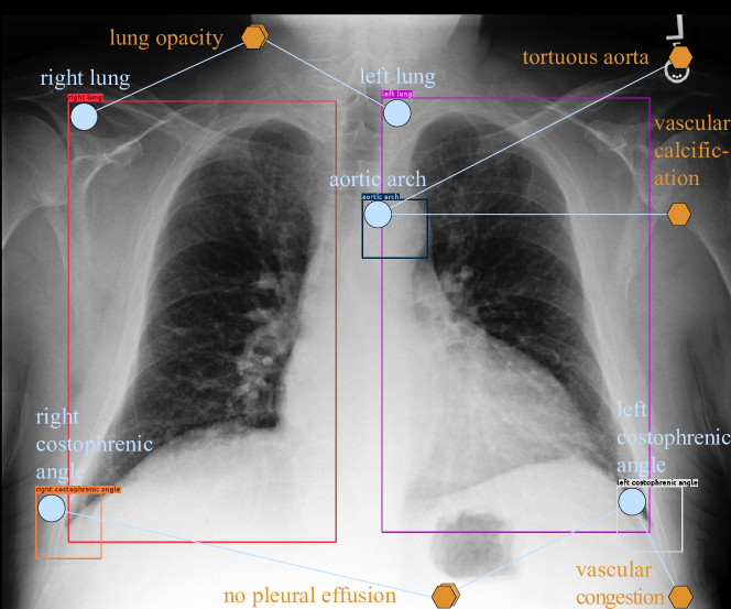
RRG is a challenging task and therefore requires adequate medical knowledge to produce a clinically accurate report. Previous studies have typically incorporated medical knowledge from external sources such as other similar images or reports [16, 17], medical entities [19], or a predefined knowledge graph [14, 38]. However, these approaches often overlook the inherent knowledge contained within each individual sample. To this end, this paper focuses more on exploring and harnessing the latent knowledge present within each sample. Scene graphs establish connections between objects and their associated attributes. As shown in Figure 1, they offer valuable source of rich contextual knowledge and high-level visual patterns. Leveraging such information is vital for writing accurate and comprehensive reports. Particularly, the radiology scene graphs used in this work are automatically generated based on both image and text, which may further introduce useful language inductive bias, thus bridging the gap between these two modalities.
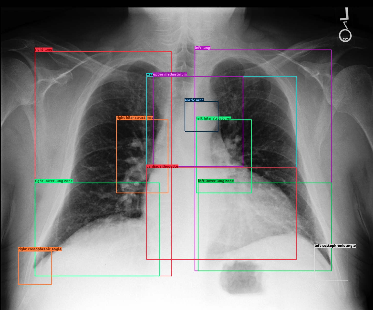
Motivated by this, we propose a novel framework called Scene Graph aided RRG (SGRRG), which leverages the automatically generated scene graph with a transformer model to reveal latent knowledge within each sample, whilst preserving the important original patch-level visual patterns. Specifically, we translate the scene graph via a carefully designed scene graph encoder and introduce a fine-grained token type embedding method to address a severe problem of overlapping anatomical regions in radiology scene graphs, as illustrated in Figure 2. The encoded scene graph, combined with the visual and textual tokens, are then fed into a scene graph-aided decoder with a fine-grained distillation attention mechanism to distill the scene graph knowledge into the model. In addition, integrates key scene-graph generation processes into its generative model, including region-level representation generation, region selection, and attribute prediction. This design renders SGRRG a highly adaptable framework, enabling the easy incorporation of other advanced RRG techniques, such as patch-level representation learning or knowledge enrichment methods. Moreover, we introduce two abnormal information learning modules to facilitate the generation of clinically accurate reports. This work makes four primary contributions:
-
1.
A novel scene graph-aided framework, SGRRG, which effectively leverages the radiology scene graph and a transformer to extract and distill valuable knowledge present in each sample for the RRG task. To the best of our knowledge, this is the first work to explore using a radiology scene graph in this way for RRG.
-
2.
Our approach can better capture the abnormal information through the incorporation of two abnormal representation learning modules, applied to images features and scene graph representations, respectively.
-
3.
Our model benefits from both global and local information, and end-to-end training, owing to its carefully designed architecture.
-
4.
SGRRG shows promising results on the largest RRG benchmark MIMIC-CXR, surpassing multiple state-of-the-art methods and exhibiting superior capabilities in capturing abnormal findings.
2 Related Works
2.1 Radiology Report Generation
Recent RRG methods follow the same encoder-decoder architecture as an image captioning (IC) task, but a significant performance gap can be seen between these two tasks, mainly due to the aforementioned problems. Some research efforts [9, 31] have been made to alleviate the problem of long text generation using the hierarchical LSTM network. Another group of works [27, 1] focus on improving the cross-modal interaction, while the most recent successful studies explore how to utilize medical domain knowledge to aid RRG. For example, Liu et al. [16] presents a model based on prior and posterior knowledge from other similar images/reports. Wang et al. [27] and Yang et al. [32] introduce disease tags to enrich abnormal and cross-modal knowledge. Zhang et al. [38] and Kale et al. [12] employ the predefined knowledge graph with the attention mechanism to generate descriptive reports. These knowledge-based approaches demonstrate improved performance on RRG, while most of them overlook the rich inherent knowledge that already exists within each sample itself. This paper therefore investigates how to leverage a radiology scene graph to extract such inherent knowledge within each sample and better aid the RRG task.
2.2 Scene Graph
Visual scene graphs [13] typically comprise the knowledge of the objects present, their associated attributes and pairwise relationship among different objects, hence encapsulating the high-level semantic contents in an image. Several computer vision tasks, e.g., image generation [11, 39] and visual question answering [22, 25], have successfully employed the scene graph and acheiving improved performance. Some studies explore it in captioning tasks where the earliest works [35, 34, 20] employ a LSTM-GNN architecture to embed the scene graph into a captioning model. To profit from a transformer model [26], one recent work [33] form a homogeneous framework by exploiting the transformer with attention mechanism to encode and translate the scene graph into image captioning. These methods have brought improvements in image captioning, but however are not appropriate to RRG as they require visual sources from a well-trained and accurate region-level feature detector. Recently, radiology scene graphs [30] were automatically established by rule-based natural language processing and a CXR atlas-based bounding box detection pipeline, leading to noisy and highly overlapped bounding box annotations in the training set. Worse still, some radiographs do not predict any anatomical location instances (objects) at the inference phase by a detector trained under these annotations, making these region-only-based scene graph methods unreliable for RRG.
To this end, we propose a new RRG framework named SGRRG which leverages the scene graph to enrich medical knowledge, while benefiting from both the global-level and patch-level image features. SGRRG contains a variety of components, each tailored to RRG for accurate report generation.
3 Methodology
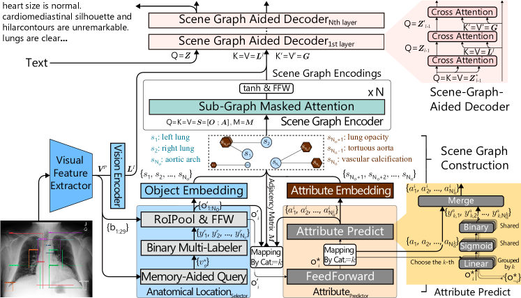
As shown in Figure 3, SGRRG comprises a visual feature extractor, a vision encoder, a scene graph construction module, a scene graph encoder, and a scene graph-aided decoder. Details of each module are given in the following sections.
3.1 Visual Feature Extractor and Vision Encoder
Let a radiology image be denoted as , the purpose of RRG is to generate coherent findings (report) from . refers to the number of words in the report. is first sent to a visual feature extractor, e.g., Swin Transformer [18], to extract the patch-level visual features which are then flattened to a sequence of visual tokens , where denotes the patch feature in the position in , and .
The vision encoder takes the extracted visual tokens as input to further capture the content and context/relationships in the image. Specifically, visual tokens are first projected into a latent space with dimension by a one-layer mapping network. These projected visual tokens are then fed into the vision encoder to perform the context modelling. Let the encoded visual tokens be denoted as .
3.2 Scene Graph Construction
Generally, a visual scene graph contains three kinds of information: objects, attributes and relationships. These nodes are connected by the following rules: (1) an object is connected to an attribute if it has this attribute, and; (2) if two objects and have a relationship, then they are connected via , denoted as . However, unlike a natural scene image, each sentence in the radiology report normally describes exactly one anatomy location (object). Hence, no explicit relationships among different objects are shown in the radiology images. The radiology scene graph therefore only contains two kinds of nodes: objects and their associated attributes. We use the automatically generated scene graph annotation from the training set to enable our proposed scene graph-aided report generation. Nevertheless, given that the scene graph is often not available during the inference phase, we incorporate a scene graph construction process into our model to generate it for the inference phase, thus creating a more adaptable, multi-task framework.
Anatomical Location Selector To generate the bounding box annotations for the inference phase, we train a detector [37] to predict the possible bounding boxes for the predefined anatomical locations defined for a radiology image, using the annotations of the training set. However, within the RRG domain, not every detected location will be described in the reports since radiologists may choose to ignore certain normal regions. Also, there is only one instance for each anatomical location in the RRG domain. To reduce spurious features, we propose to perform a multi-label binary classification task to predict whether an anatomical location should be included in the scene graph. In detail, a linear layer with a Sigmoid function is applied to the average-pooled visual feature :
| (1) |
where is the learnable weight and denotes the total number of anatomical locations (object categories). is a threshold function mapping inputs larger than to , and 0 otherwise. , indicates the inclusion of anatomical location. Only anatomical locations detected by the detector with a are included in the scene graph.
Despite the use of binary classification, filtering out the irrelevant anatomical locations purely based on the image is still difficult. Inspired by [1] in learning the cross-modal patterns, we design a memory-aided region selector by employing a memory matrix and performing a query-response process to distil the prior knowledge into the selector. In particular, we randomly initialize a learnable memory matrix that records the region selection knowledge across images. To distil the prior knowledge into the current image, we perform a query and response process that selects the top relevant memory slots (query) from the memory matrix and fuses them with the visual features (response). Specifically, we first project the global visual feature into the same latent space as memory matrix: . The similarity between each memory slot and is calculated by Equation 2. Then, the top memory slots with the highest similarities are selected to generate the response for the image:
| (2) | ||||
| (3) |
where is the row of ; , and are three learnable weights. denotes the weight of the memory slot. After obtaining the response , we fuse the global visual feature with the response by concatenating them with a lightweight, feed-forward module:
| (4) |
where is the activation. This prior-knowledge-enriched feature is the one finally fed into the Equation 1 to perform the anatomical location selection.
Attribute Predictor With the anatomical locations on hand, the next step is to predict the attributes associated with them, which collaboratively form the final scene graph at the inference phase. Similarly, this is achieved by integrating a multi-label attribute classification task into the model. Since the number of attributes varies between different anatomical locations, each anatomical location is equipped with a separate classification head. We apply this classification to each selected instance of the anatomical location in the image. An instance representation is denoted as (details how it is obtained from the bounding-box annotation is given below), the prediction of its relevant attribute is :
| (5) | ||||
| (6) |
where is fed into a one-layer feed-forward module followed by the classification head to predict the presence () of the attribute in anatomical location (category) . Here, , and denote the weights and the number of attribute categories for the anatomical location , respectively.
3.3 Scene Graph Encoder
This section presents the details of how we translate the radiology scene graph into the RRG model.
Object and Attribute Embedding Given the bounding box and attribute annotations, we aim to generate dense object and attribute embeddings. Specifically, we apply the Region-of-Interest pooling [7] to visual features based on the bounding-box annotations to obtain the initial region-level object embedding . Here, refers to the number of objects described in a radiology image. After this step, a one-layer feed-forward module is employed to improve the object representation by mapping it into the same latent space as the Vision Encoder and Decoder. The procedure to obtain the object embedding can be expressed as:
| (7) | ||||
| (8) |
To obtain the attribute embedding, we map each attribute to a unique index number through a mapping function and employ a trainable embedding layer to embed it into the same latent space as the object embedding. A layer normalization and a dropout layer are used to improve the robustness of the representation learning further:
| (9) | ||||
| (10) |
where and denote the attribute and embedded attribute for object in image respectively, e.g., lung opacity for object right lung. is the number of attributes for the object. Note that differs depending on the type of object.
Scene Graph Encoding We employ an attention mechanism [26] to gauge co-occurrences and learn the contextual knowledge of the embeddings. Akin to [33] who replaces a GNN with homogeneous Transformers, we adopt the Transformer architecture to encode the scene graph after obtaining the original embeddings. Specifically, given the object embeddings and attribute embeddings , we first append attribute embeddings to object embeddings to form a sequence of node tokens. Then, a trainable token-type embedding is added to enable the encoder to recognize the type of tokens:
| (11) | |||||
| (12) |
The final node token set, , comprises both object embeddings and their associated attribute embeddings, where . However, as shown in Figure 2, objects in the radiology image are normally highly overlapped. This hinders the encoder’s ability to discern distinct objects and impedes the learning of contextual knowledge. Possible noisy box annotations further exacerbate this problem. To tackle this, we propose applying a fine-grained token-type embedding, namely anatomy embedding. We add to the object embeddings with a learnable token-type embedding for each anatomical category. Equation 11 then becomes 13 where indexes the anatomical category for the object and denotes the token type embedding for anatomical category .
| (13) |
After obtaining the initial node tokens, the next step is to encode the topology of the graph. We utilize the attention mask to depict the connectivity of nodes. In particular, we mark if node and are connected directly in the original scene graph, otherwise . Note that is a symmetric matrix, i.e., , analogous to an adjacency matrix. The node tokens together with this attention mask are then fed into the scene graph encoder consisting of several transformer blocks to perform the scene graph encoding. Through the attention mask , each position of the higher Transformer layer mask-attend to the visible positions of the lower layer, acting as a graph aggregator, as expressed in Equation 14. In this way, the scene-graph encoder can model the long-range dependency between connected nodes and capture the topology. Thus:
| (14) |
where are the node tokens, denotes node tokens after masked-attention. is the Hadamard product operation. We denote the topology-enriched scene graph embeddings as output by the final layer of the encoder.
Scene Graph Aided Decoder Given the report , the encoded visual tokens and the encoded scene graph , we are able to train a mapping between them with a decoder which performs cross-modal fusion and autoregressively generates the report word by word. Here, we propose a transformer-based scene graph aided decoder to further distill the encoded scene graph into the model with that cross-attend to the interleaved inputs. In particular, an embedding layer is first created through tokenization to produce a sequence of dense representations of the report . Then, in each transformer block222we omit the and after each attention layer for clarity., we perform a self-attention within textual tokens , a cross-attention between textual tokens and visual tokens, and finally a cross-attention between the visual-enriched textual tokens and scene graph representation as expressed below:
| (15) | ||||
| (16) | ||||
| (17) |
where denotes the textual tokens output from the transformer layer and is the initial embedded textual tokens. The textual tokens first interact with all visual tokens to absorb basic visual information, which may contain noisy and unimportant knowledge. Then, we further distill the scene graph encapsulating the essential visual information and context knowledge into the textual tokens. Through this coarse-to-fine scenario, the model benefits from global, local, and context knowledge.
As mentioned above, no explicit relationship is shown among different objects in the automatically generated scene graph. Hence, each scene graph actually consists of several sub-graphs which typically contain one anatomical location instance and its associated attributes, and corresponds to one sentence in the report. This observation inspired us to design a more fine-grained way to distill the scene graph. Intuitively, instead of requiring the model to find the important information from a scene graph representation containing both the object and attribute nodes from different anatomical locations for each textual token, it is relatively easier to learn useful information from a structured and refined representation, especially for RRG scene graph where each anatomical location instance generally has attributes and one scene graph may contain more than node tokens. To achieve this, we propose a sub-graph (sentence) level attention by utilizing max-pooling to encapsulate the core knowledge in each sub-graph and then distilling them into the model:
| (18) | ||||
| (19) |
where , are the object tokens and its attribute token output by the scene graph encoder for anatomical location. Through the sub-graph attention, we explicitly alleviate the possible negative influence from other nodes (sentences) where the number of tokens from other sub-graphs (sentences) could reduce from more than to less than .
3.4 Abnormal Information Learning
Information about abnormalities plays a vital role in generating clinically accurate reports. In this paper, we employ disease recognition and normal-abnormal segregation modules to enrich the abnormal information in the model.
Disease Recognition: As no ground-truth disease labels are available in the commonly used RRG benchmarks, we utilize pseudo-labels generated by an automatic labeller [8] predicting 14 diseases on chest radiographs (shown in the supplementary file) to form a multilabel disease recognition task. In detail, we apply this task to the average-pooled visual features via a simple linear classification head, since the performance of the whole generative model is highly dependent on the quality of the extracted visual feature.
Normal-Abnormal Segregation (NAS): We also expect that our scene graph can better capture the abnormal information. To achieve this, we first leverage the attribute information to generate the abnormality label for each sub-graph. All attributes belong to seven predefined types (listed in the supplementary file) and two of them could indicate the sample abnormality: (1) anatomical finding attribute with template ‘{yes,no}disease’ such as ‘yespneumothorax’; (2) NLP attribute with template ‘{yes,no}{normal, abnormal}’. After obtaining the abnormality label, we use contrastive learning to improve abnormal scene graph representation learning. Note that, instead of classification, we choose contrastive learning as it is relatively soft and more appropriate for RRG given that the automatically generated scene graph may contain noisy and inaccurate supervision. We employ this contrastive learning to the global sub-graph representation and Equation 20 shows the calculation of the contrastive loss for the anatomical location .
| (20) | ||||
where and denote the cosine similarity and normalization functions; and are the global sub-graph representation calculated by Equation 18 from the same anatomical location in one batch; and is the number of sub-graphs from anatomical location in one batch and is the margin and set to . By using this contrastive loss, we improve the scene graph abnormal representation learning by segregating the normal-abnormal information. Note that any contrastive loss can be applied here.
3.5 Objective Function
Given the final textual tokens output by the decoder, a cross entropy loss is used to supervise the report generation task, as shown in Equation 21, where and denotes the the classification head and the ground truth label for word in the report. Our model is jointly optimized by report generation loss , region selection loss , the attribute prediction loss , the disease recognition loss and the normal-abnormal segregation loss . The region selection and attribute prediction losses are implemented by the cross-entropy loss. Equation 22 shows the final loss :
| (21) | ||||
| (22) |
where and are the hyper-parameters to control the contributions of different losses. One may ask why we do not directly use region features or the scene graph as the only visual source and remove the visual feature extractor. We address this question in a discussion in the supplementary files.
| Method | BL-1 | BL-2 | BL-3 | BL-4 | MTOR | RG-L | P | R | F1 |
| 0.308 | 0.196 | 0.137 | 0.102 | 0.131 | 0.272 | 0.285 | 0.195 | 0.193 | |
| 0.378 | 0.247 | 0.175 | 0.132 | - | 0.306 | 0.422 | 0.212 | 0.234 | |
| 0.331 | 0.207 | 0.145 | 0.108 | 0.132 | 0.266 | 0.365 | 0.225 | 0.235 | |
| 0.385 | 0.251 | 0.178 | 0.133 | 0.151 | 0.313 | 0.376 | 0.203 | 0.219 | |
| 0.385 | 0.252 | 0.178 | 0.133 | 0.151 | 0.315 | 0.357 | 0.215 | 0.218 | |
| 0.399 | 0.240 | 0.159 | 0.112 | 0.147 | 0.289 | 0.260 | 0.195 | 0.152 | |
| 0.381 | 0.249 | 0.176 | 0.131 | 0.153 | 0.315 | 0.410 | 0.244 | 0.268 | |
| 0.394 | 0.257 | 0.182 | 0.136 | 0.161 | 0.323 | 0.360 | 0.206 | 0.209 | |
| 0.373 | 0.249 | 0.175 | 0.126 | 0.168 | 0.264 | 0.380 | 0.318 | 0.305 | |
| 0.434 | 0.285 | 0.202 | 0.149 | 0.173 | 0.326 | 0.440 | 0.323 | 0.332 |
4 Experiments
4.1 Dataset and Evaluation Metrics
We verify the effectiveness of our method in the Chest ImaGenome dataset [30] which is derived from the most widely used and largest RRG benchmark, i.e., MIMIC-CXR [10], consisting of chest X-ray images with free-text reports. The Chest ImaGenome dataset provides automatically constructed scene graphs for the MIMIC-CXR frontal radiography where each scene graph contains bounding-box annotations for 29 unique anatomical locations, their associated attributes, and a label indicating if an anatomical location is described in the report. We adopt the official data split and follow previous works [24, 27] to discard reports with empty finding sections, resulting in 113,473 training images, 16498 validation images and 32711 test images.
We use six commonly used natural language processing metrics, i.e., BLEU{1-4} [21], Rouge-L [15] and METEOR [5], to measure the performance of our model. To measure the model’s capability of capturing the abnormalities, we follow previous works to report the clinical efficacy metric where CheXbert [23] is applied to labeling the generated reports and the results are compared with ground truth in 14 disease categories. We use macro-average precision, recall, and F1 score to measure clinical efficacy.
4.2 Implementation details
We adopt the Swin-B [18] pre-trained on ImageNet2K [4] as our visual feature extractor. The vision encoder, scene-graph encoder, and scene-graph-aided decoder are randomly initialized comprising three transformer layers with a hidden size of and an attention head of . The weights , , , to control the loss contributions in Equation 22 are set to , , , . Further implementation details, e.g., data augmentation and learning rates, are given in the supplementary files.
4.3 Comparison to SOTA methods
Here, we compare our method with two representative image captioning models [36] and [3], one recent pretrained vision-language model [6], and recent state-of-the-art RRG studies including [2], [1], [27], [32], [29] and [24]. As shown in Table 1, achieves the best performance in all the NLP metrics, especially for BLEU score where our method surpasses the second-best performing method by a large margin (+ 3.5% in B1 and +1.3% in B4). In addition, also outperforms previous methods in all clinical efficacy metrics, demonstrating that it can better capture abnormal observations and produce clinically accurate reports. The method takes the bounding boxes features as the only visual source, hence showing good performance in clinical efficacy than other previous methods, e.g., , , and which consider the learnable patch-level visual features as input. However, since loses important global information, it fails to produce the same coherent reports as other patch-level feature-based approaches, as indicated by NLP metrics. Nonetheless, obtains promising results on both the NLP and clinical efficacy metrics. We mainly attribute this to the rich context and domain knowledge in the scene graph and its bespoke architecture which takes the best advantage of both the global and local information with abnormal information enrichment. Note that the region-level features in are derived from the patch-level features, hence they are jointly optimised during the training, rather than fixed bounding box features that heavily rely on a specific detector and accurate annotations.
| Method | BL1 | BL4 | MTR | RG | AVG. | P | R | F1 | AVG. |
|---|---|---|---|---|---|---|---|---|---|
| 0.381 | 0.134 | 0.153 | 0.318 | - | 0.388 | 0.241 | 0.257 | - | |
| 0.434 | 0.149 | 0.173 | 0.326 | +% | 0.446 | 0.324 | 0.333 | +% | |
| w/o | 0.386 | 0.135 | 0.153 | 0.317 | +% | 0.420 | 0.244 | 0.262 | +% |
| w/o | 0.427 | 0.142 | 0.170 | 0.319 | +% | 0.406 | 0.327 | 0.330 | +% |
| w/o | 0.412 | 0.140 | 0.166 | 0.322 | +% | 0.418 | 0.321 | 0.328 | +% |
| w/o | 0.427 | 0.142 | 0.170 | 0.318 | +% | 0.439 | 0.318 | 0.336 | +% |
| w/o | 0.418 | 0.141 | 0.167 | 0.323 | +% | 0.410 | 0.314 | 0.320 | +% |
| w/o | 0.421 | 0.141 | 0.169 | 0.323 | +% | 0.422 | 0.282 | 0.301 | +% |
4.4 Ablation Studies
Contribution of each component We conduct an ablation study to investigate the contribution of each proposed core module in SGRRG. Specifically, the model consists of the visual extractor and the transformer as the vision encoder and decoder. We verify the performance improvements brought by six components: (1) SG: The whole scene graph design. (2) SgAtt: The Subgraph-level ATTention (3) DR: The disease recognition; (4) NAS: The Normal-Abnormal Segregation. (5) AE: The fine-grained Anatomy Embedding. (6) MEM: The MEMory mechanism in region selection.
As presented in Table 2, improves remarkably the performance of model on both the NLP and clinical efficacy metrics (+10.2% and +26.3% on average over all NLP and clinical efficacy metrics, respectively). Furthermore, each component of SGRRG can be found to have a positive effect on overall performance. Specifically, a significant performance drop can be seen when we remove the whole scene graph design meaning that current model resorts to . These results verify the effectiveness of our scene-graph-aided design and confirm the theory of leveraging the radiology scene graph as a knowledge source. In addition, removing the , and notably impedes the model performance on NLP metrics, while showing relatively modest influence on the clinical efficacy since these designs focus more on improving the scene graph representation. A more obvious performance drop is reported when the module is removed, indicating the importance of alleviating the overlapping issues in noisy radiology scene graphs. Furthermore, segregating abnormal-normal sub-graphs and enriching visual features with disease information play an essential role in model performance, especially for clinically accurate report generation, as evidenced by comparing the last two rows with .
| Method | BL1 | BL4 | MTR | RG | P | R | F1 |
|---|---|---|---|---|---|---|---|
| 0.421 | 0.144 | 0.169 | 0.325 | 0.440 | 0.324 | 0.323 | |
| 0.434 | 0.149 | 0.173 | 0.326 | 0.446 | 0.324 | 0.333 |
4.4.1 Average Pooling vs Maximum Pooling
: We apply the maximum pooling in our sub-graph level attention and normal-abnormal segregation modules to obtain sentence-level representation. Here, we conduct an ablation study to explore the effect of average pooling and maximum pooling. It can be found from Table 3 that with maximum pooling obtains better performance in both the NLP and clinical efficacy metrics. This is expected as the pooling highlights the salient parts in a sub-graph which is more suitable for fine-grained distillation modules and abnormal information learning, while the average pooling may diminish the contribution for those salient parts. Further ablation studies, e.g., the capacity of the memory matrix and the margin in the NAS module, are shown in the supplementary files.
4.5 Qualitative Results
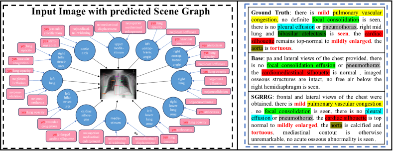
We present qualitative results to further demonstrate the effectiveness of . As illustrated in Figure 4, appears to better capture disease information and generate abnormal descriptions, e.g., “there is mild pulmonary vascular congestion, the cardiac silhouette is top normal to mildly enlarged and the aorta is calcified and tortuous.”, compared to the model. To investigate whether this improvement is truly related to the radiology scene graph, we also visualize the predicted scene graphs with anatomical finding attributes in which the abnormal observations, e.g., “lung opacity", “atelectasis", “vascular congestion" and “tortuous aorta", are present. Clearly, such abnormal medical observations are vital in report generation. Moreover, the average number of words in reports generated by is % longer than the base model, i.e., vs ( in ground truth reports), indicating that could generate more descriptive reports. These results further verify the potential of the radiology scene graph and our proposed framework. Further examples are given in the supplementary files.
4.6 Limitations
Although we incorporate the core scene graph generation modules into the model to generate the scene graphs purely based on the image in the inference phase where reports are unavailable for scene graph mining required by recent automatic tools in radiology domain, our framework still depends on automatic tools to extract the scene graphs from the training set during training. Moreover, to attain enhanced performance, SGRRG necessitates an ancillary phase encompassing the construction and encoding of the scene graphs, and the abnormal information enrichment, which consequently prolongs the training time by % per epoch. While the increment in testing is small (+%), mainly attributed to the elimination of additional gradient computations associated with the losses from graph construction and abnormal information enrichment during the inference phase. Further code optimization may diminish the extra time cost.
5 Conclusion
We propose a novel RRG framework that harnesses the inherent knowledge within each sample by transforming the radiology scene graph into the model. A scene graph encoder is designed to encode the scene graph and alleviates the overlapping problem shown in the radiology domain. We construct a scene graph-aided decoder to distill the encoded scene graph into the model. integrates the scene graph generation into the model and takes advantage of visual patterns at the patch and region levels, forming a more flexible architecture through carefully designed modules. Extensive experiments verify the superior performance of and validate the effectiveness of each proposed module. This work also demonstrates the great potential knowledge that exists within each sample and presents an effective approach to leverage radiology scene graphs as an in-sample knowledge source.
References
- [1] Chen, Z., Shen, Y., Song, Y., Wan, X.: Cross-modal memory networks for radiology report generation. In: Proceedings of the 59th Annual Meeting of the Association for Computational Linguistics and the 11th International Joint Conference on Natural Language Processing (Volume 1: Long Papers). pp. 5904–5914 (2021)
- [2] Chen, Z., Song, Y., Chang, T.H., Wan, X.: Generating radiology reports via memory-driven transformer. In: Proceedings of the 2020 Conference on Empirical Methods in Natural Language Processing (EMNLP). pp. 1439–1449 (2020)
- [3] Cornia, M., Stefanini, M., Baraldi, L., Cucchiara, R.: Meshed-memory transformer for image captioning. In: Proceedings of the IEEE Conference on Computer Vision and Pattern Recognition. pp. 10578–10587 (2020)
- [4] Deng, J., Dong, W., Socher, R., Li, L.J., Li, K., Fei-Fei, L.: Imagenet: A large-scale hierarchical image database. In: 2009 IEEE Conference on Computer Vision and Pattern Recognition. pp. 248–255. Ieee (2009)
- [5] Denkowski, M., Lavie, A.: Meteor 1.3: Automatic metric for reliable optimization and evaluation of machine translation systems. In: Proceedings of the sixth workshop on Statistical Machine Translation. pp. 85–91 (2011)
- [6] Dou, Z.Y., Kamath, A., Gan, Z., Zhang, P., Wang, J., Li, L., Liu, Z., Liu, C., LeCun, Y., Peng, N., et al.: Coarse-to-fine vision-language pre-training with fusion in the backbone. Advances in neural information processing systems 35, 32942–32956 (2022)
- [7] Girshick, R.: Fast r-cnn. In: Proceedings of the IEEE International Conference on Computer Vision. pp. 1440–1448 (2015)
- [8] Irvin, J., Rajpurkar, P., Ko, M., Yu, Y., Ciurea-Ilcus, S., Chute, C., Marklund, H., Haghgoo, B., Ball, R., Shpanskaya, K., et al.: Chexpert: A large chest radiograph dataset with uncertainty labels and expert comparison. In: Proceedings of the AAAI conference on artificial intelligence. vol. 33, pp. 590–597 (2019)
- [9] Jing, B., Xie, P., Xing, E.: On the automatic generation of medical imaging reports. In: Proceedings of the 56th Annual Meeting of the Association for Computational Linguistics (Volume 1: Long Papers). pp. 2577–2586 (2018)
- [10] Johnson, A.E., Pollard, T.J., Greenbaum, N.R., Lungren, M.P., Deng, C.y., Peng, Y., Lu, Z., Mark, R.G., Berkowitz, S.J., Horng, S.: Mimic-cxr-jpg, a large publicly available database of labeled chest radiographs. arXiv preprint arXiv:1901.07042 (2019)
- [11] Johnson, J., Gupta, A., Fei-Fei, L.: Image generation from scene graphs. In: Proceedings of the IEEE conference on Computer Vision and Pattern Recognition. pp. 1219–1228 (2018)
- [12] Kale, K., Bhattacharyya, P., Gune, M., Shetty, A., Lawyer, R.: Kgvl-bart: Knowledge graph augmented visual language bart for radiology report generation. In: Proceedings of the 17th Conference of the European Chapter of the Association for Computational Linguistics. pp. 3393–3403 (2023)
- [13] Krishna, R., Zhu, Y., Groth, O., Johnson, J., Hata, K., Kravitz, J., Chen, S., Kalantidis, Y., Li, L.J., Shamma, D.A., et al.: Visual genome: Connecting language and vision using crowdsourced dense image annotations. International journal of computer vision 123, 32–73 (2017)
- [14] Li, C.Y., Liang, X., Hu, Z., Xing, E.P.: Knowledge-driven encode, retrieve, paraphrase for medical image report generation. In: Proceedings of the AAAI Conference on Artificial Intelligence. vol. 33, pp. 6666–6673 (2019)
- [15] Lin, C.Y.: Rouge: A package for automatic evaluation of summaries. In: Text Summarization Branches Out. pp. 74–81 (2004)
- [16] Liu, F., Wu, X., Ge, S., Fan, W., Zou, Y.: Exploring and distilling posterior and prior knowledge for radiology report generation. In: Proceedings of the IEEE Conference on Computer Vision and Pattern Recognition. pp. 13753–13762 (2021)
- [17] Liu, F., Yin, C., Wu, X., Ge, S., Zhang, P., Sun, X.: Contrastive attention for automatic chest x-ray report generation. In: Findings of the Association for Computational Linguistics: ACL-IJCNLP 2021. pp. 269–280 (2021)
- [18] Liu, Z., Lin, Y., Cao, Y., Hu, H., Wei, Y., Zhang, Z., Lin, S., Guo, B.: Swin transformer: Hierarchical vision transformer using shifted windows. In: Proceedings of the IEEE international Conference on Computer Vision. pp. 10012–10022 (2021)
- [19] Miura, Y., Zhang, Y., Tsai, E., Langlotz, C., Jurafsky, D.: Improving factual completeness and consistency of image-to-text radiology report generation. In: Proceedings of the 2021 Conference of the North American Chapter of the Association for Computational Linguistics: Human Language Technologies. pp. 5288–5304 (2021)
- [20] Nguyen, K., Tripathi, S., Du, B., Guha, T., Nguyen, T.Q.: In defense of scene graphs for image captioning. In: Proceedings of the IEEE International Conference on Computer Vision. pp. 1407–1416 (2021)
- [21] Papineni, K., Roukos, S., Ward, T., Zhu, W.J.: Bleu: a method for automatic evaluation of machine translation. In: Proceedings of the 40th annual meeting of the Association for Computational Linguistics. pp. 311–318 (2002)
- [22] Shi, J., Zhang, H., Li, J.: Explainable and explicit visual reasoning over scene graphs. In: Proceedings of the IEEE conference on Computer Vision and Pattern Recognition. pp. 8376–8384 (2019)
- [23] Smit, A., Jain, S., Rajpurkar, P., Pareek, A., Ng, A.Y., Lungren, M.: Combining automatic labelers and expert annotations for accurate radiology report labeling using bert. In: Proceedings of the 2020 Conference on Empirical Methods in Natural Language Processing (EMNLP). pp. 1500–1519 (2020)
- [24] Tanida, T., Müller, P., Kaissis, G., Rueckert, D.: Interactive and explainable region-guided radiology report generation. In: Proceedings of the IEEE Conference on Computer Vision and Pattern Recognition. pp. 7433–7442 (2023)
- [25] Teney, D., Liu, L., van Den Hengel, A.: Graph-structured representations for visual question answering. In: Proceedings of the IEEE conference on Computer Vision and Pattern Recognition. pp. 1–9 (2017)
- [26] Vaswani, A., Shazeer, N., Parmar, N., Uszkoreit, J., Jones, L., Gomez, A.N., Kaiser, Ł., Polosukhin, I.: Attention is all you need. Advances in Neural Information Processing Systems 30 (2017)
- [27] Wang, J., Bhalerao, A., He, Y.: Cross-modal prototype driven network for radiology report generation. In: Computer Vision–ECCV 2022: 17th European Conference, Tel Aviv, Israel, October 23–27, 2022, Proceedings, Part XXXV. pp. 563–579. Springer (2022)
- [28] Wang, J., Bhalerao, A., Yin, T., See, S., He, Y.: Camanet: Class activation map guided attention network for radiology report generation. arXiv preprint arXiv:2211.01412 (2022)
- [29] Wang, J., Bhalerao, A., Yin, T., See, S., He, Y.: Camanet: class activation map guided attention network for radiology report generation. IEEE Journal of Biomedical and Health Informatics (2024)
- [30] Wu, J., Agu, N., Lourentzou, I., Sharma, A., Paguio, J.A., Yao, J.S., Dee, E.C., Kashyap, S., Giovannini, A., Celi, L.A., et al.: Chest imagenome dataset for clinical reasoning. In: Annual Conference on Neural Information Processing Systems (2021)
- [31] Xue, Y., Huang, X.: Improved disease classification in chest x-rays with transferred features from report generation. In: Information Processing in Medical Imaging: 26th International Conference, IPMI 2019, Hong Kong, China, June 2–7, 2019, Proceedings 26. pp. 125–138. Springer (2019)
- [32] Yang, S., Wu, X., Ge, S., Zheng, Z., Zhou, S.K., Xiao, L.: Radiology report generation with a learned knowledge base and multi-modal alignment. Medical image analysis 86, 102798 (2023)
- [33] Yang, X., Peng, J., Wang, Z., Xu, H., Ye, Q., Li, C., Yan, M., Huang, F., Li, Z., Zhang, Y.: Transforming visual scene graphs to image captions. In: Proceedings of the 61th Annual Meeting of the Association for Computational Linguistics (Volume 1: Long Papers) (2023)
- [34] Yang, X., Zhang, H., Cai, J.: Auto-encoding and distilling scene graphs for image captioning. IEEE Transactions on Pattern Analysis and Machine Intelligence 44(5), 2313–2327 (2020)
- [35] Yao, T., Pan, Y., Li, Y., Mei, T.: Exploring visual relationship for image captioning. In: Proceedings of the European conference on computer vision (ECCV). pp. 684–699 (2018)
- [36] Zeng, P., Zhu, J., Song, J., Gao, L.: Progressive tree-structured prototype network for end-to-end image captioning. In: Proceedings of the 30th ACM International Conference on Multimedia. pp. 5210–5218 (2022)
- [37] Zhang, H., Li, F., Liu, S., Zhang, L., Su, H., Zhu, J., Ni, L., Shum, H.Y.: Dino: Detr with improved denoising anchor boxes for end-to-end object detection. In: The Eleventh International Conference on Learning Representations (2022)
- [38] Zhang, Y., Wang, X., Xu, Z., Yu, Q., Yuille, A., Xu, D.: When radiology report generation meets knowledge graph. In: Proceedings of the AAAI Conference on Artificial Intelligence. vol. 34, pp. 12910–12917 (2020)
- [39] Zhao, B., Meng, L., Yin, W., Sigal, L.: Image generation from layout. In: Proceedings of the IEEE Conference on Computer Vision and Pattern Recognition. pp. 8584–8593 (2019)
See pages 1-4 of ECCV2024_ID459_supp.pdf