A Spectral Element Enrichment Wall-Model

Abstract

We develop an enrichment wall-model within the spectral element method (SEM) framework for large-eddy simulations of wall-bounded flows. The method augments the polynomial solution in the wall-adjacent elements with an analytical law-of-the-wall enrichment function representing the mean velocity near the wall. In the solution representation, this enrichment function captures the large gradients in the boundary layer, which allows the polynomial modes to represent the turbulent fluctuations. The enriched solution is able to resolve the shear stress at the wall without any modification to the no-slip wall boundary conditions. The performance of the SEM enrichment wall-modeling approach is assessed in turbulent channel flow LES for a range of Reynolds numbers. The results show that the proposed method improves solution accuracy on under-resolved near-wall grids as compared to the traditional shear stress wall-models.

1 Introduction

High Reynolds number turbulent flows are a norm, not the exception in engineering systems. Correctly simulating turbulent wall-bounded flows is crucial for applications, such as turbomachinery and internal combustion engines [1]. In such applications, accurately resolving the velocity and thermal boundary layers at the wall is critical to compute the quantities of interest. However, prohibitive costs render computational fluid dynamics (CFD) simulations of these full-scale systems infeasible because they need to resolve smallest turbulent eddies.

For most industry-relevant flow problems, this computational cost issue is addressed by using Reynolds-Averaged Navier-Stokes (RANS) simulations wherein all turbulent length and time scales are modeled and the mean flow solution is computed. For some problems, these methods are sufficient, but for unsteady simulations, simulations with flow separation, and flows with laminar-to-turbulent transition, RANS methods are unreliable. For such problems, the turbulent scales must be resolved throughout the domain in direct numerical simulations (DNS), or in the near-wall regions and modeled elsewhere in wall-resolved large-eddy simulations (WRLES). However, both of these approaches are computationally infeasible because the number of grid points in the near-wall region scales with $Re_{\tau}^{2}$ [2]. Hence, there is a need to develop reliable methods to reduce the cost of such simulations by modeling the smaller turbulent scales in the near-wall regions, but resolving the large-scale transients via wall-modeled large eddy simulations (WMLES).

There have been a number of different WMLES algorithms developed in the literature. Most have been developed for finite-difference (FD) and finite-volume (FV) methods [3], but recently there have been efforts to develop such methods in the context of higher-order methods such as the Spectral Element Method (SEM) [4], Spectral Difference Method (SDM) [5], and the discontinuous Galerkin (DG) method [6] [7] [8]. Most of these methods use the solution outside of the near-wall region to fit an empirical wall function in the boundary layer in order to compute the wall shear stress. Then, this shear stress is applied to the flow as the wall boundary condition. In the context of DG and continuous finite element method (FEM), there have been efforts to develop so-called enriched basis turbulence wall models [8] [9] [10] [11] [12]. These methods augment the solution by considering the empirical wall function as part of the solution representation. Doing so removes spurious oscillations in the near-wall region due to insufficient polynomial resolution of the boundary layer and improves the solution representation by allowing the degrees of freedom to represent the flow fluctuations instead of the mean flow behavior.

In the present work, a first-of-its-kind enriched basis WMLES approach for high-order SEM is developed and its performance is compared against the traditional equilibrium wall-stress modeling framework. The method is designed to improve the accuracy of the WMLES, prevent unphysical oscillations, and be easily implementable in existing SEM solvers. Specifically, this method is implemented in the high-order SEM CFD solver Nek5000 [13]. The method is validated in the context of WMLES calculations for test problems pertaining to turbulent channel flows.

2 Governing Equations

We consider incompressible, Newtonian flows as governed by the Navier-Stokes equations:

$$\frac{\partial\bm{u}}{\partial t} =-\nabla p+\nabla\cdot\left[\nu\left(\nabla\bm{u}+\nabla\bm{u}^{T}\right)\right]-\bm{u}\cdot\nabla\bm{u}$$ (1)

$$\nabla\cdot\bm{u} =0$$ (2)

where $\bm{u}$ is the velocity vector, $t$ corresponds to time, $p$ is the pressure, and $\nu$ is kinematic viscosity of the fluid. The equations are solved over a computational domain $\Omega$ with boundary $\partial\Omega$.

3 Spectral Element Method

The governing equations are discretized using the spectral element method (SEM) in the Nek5000 [13] solver. In the SEM, the governing equations are put into a weighted residual formulation by multiplying Eqs. (1)-(2) by test functions $\bm{v}$ and $q$, respectively, and integrating over the elements, so the goal is to find $(\bm{u},p)\in X_{b}^{P}(\Omega)\times Y^{P}(\Omega)$ such that

$$\frac{d}{dt}(\bm{v},\bm{u}) =-\left(\bm{v},\frac{1}{\rho}\nabla p\right)+(\bm{v},\nabla\cdot\nu(\nabla\bm{u}+\nabla\bm{u}^{T}))-(\bm{v},\bm{u}\cdot\nabla\bm{u}),$$ (3)

$$(\nabla\cdot\bm{u},q) =0,$$ (4)

for all test functions $(\bm{v},q)\in X_{0}^{P}(\Omega)\times Y^{P}(\Omega)$, where the $\mathcal{L}^{2}$ inner product is defined as $(\bm{f},\bm{g})\coloneqq\int_{\Omega}\bm{f}\cdot\bm{g}\,dV$. Here, $X^{P}(\Omega)\subset H^{1}(\Omega)$ is the set of continuous $P$th-order spectral element basis functions. $X^{P}_{b}$ is the subset of $X^{P}$ such that Dirichlet boundary conditions are satisfied on the boundary, $\partial\Omega$. The subset satisfying homogeneous Dirichlet boundary conditions is $X^{P}_{0}$. Similarly, $Y^{P}(\Omega)\subset H^{1}(\Omega)$ is the set of continuous $P$th-order spectral element basis functions [14]. The specifics of these basis functions will be defined later in this section, because the development of the weak form does not depend on the specific basis. From here, Eqs. (3)-(4) are integrated by parts to reduce the derivative on $\bm{u}$ and create a symmetric form. This gives the final weighted residual form:

$$\frac{d}{dt}(\bm{v},\bm{u}) =\left(\nabla\cdot\bm{v},\frac{1}{\rho}p\right)-(\nabla\bm{v},\nu(\nabla\bm{u}+\nabla\bm{u}^{T}))-(\bm{v},\bm{u}\cdot\nabla\bm{u}),$$ (5)

$$(\nabla\cdot\bm{u},q) =0.$$ (6)

The $\mathbb{P}^{P}-\mathbb{P}^{P}$ velocity-pressure spaces are used [14]. The discretization up to this point is equivalent to a continuous finite-element discretization, but what separates SEM is the particular choice of basis and quadrature rule that will be discussed next.

Globally, each component of the velocity is represented on a Lagrange interpolating basis:

$$u(\bm{x})=\sum_{i=1}^{N_{c}}\underline{u}_{i}\phi_{i}(\bm{x}),$$ (7)

where $\underline{u}$ is the vector of basis coefficients, $\underline{u}_{i}$ is the $i$^th basis coefficient, $\phi_{i}(\bm{x})$ are continuous basis functions on $\Omega$, and $N_{c}$ is the total number of coefficients for all basis functions. This form is also used for the pressure.

In practice, the global form of the solution is never used. Instead, the domain, $\Omega$, is partitioned into $N_{e}$ non-overlapping discrete elements such that $\Omega=\cup_{e=1}^{N_{e}}\Omega_{e}$ and the solution is represented with local basis functions such that $\phi_{i}^{e}$ is non-zero in element $e$ and zero everywhere else. In this study, only tensor-product elements are used. Within each element the basis functions are formed by isoparametrically mapping the element to a reference element $\widehat{\Omega}\coloneqq[-1,1]^{d}$ with dimension, $d$, as schematically shown in Fig. 1 [14]. From there, the solution is approximated by a high-order polynomial of order $P$:

$$u=\sum_{i=1}^{N_{b}}\underline{u}^{e}_{i}\phi^{e}_{i}(\bm{x})=\sum_{i=1}^{P+1}\sum_{j=1}^{P+1}\sum_{k=1}^{P+1}\underline{u}^{e}_{ijk}h_{i}(r)h_{j}(s)h_{k}(t),$$ (8)

where $N_{b}=(P+1)^{d}$ is the number of basis functions in an element, $d$ is the dimension of the problem, and $h_{i}$ is the $i$^th 1D basis function used in the tensor product. In general, the 1D basis functions could be any set of polynomial basis functions.

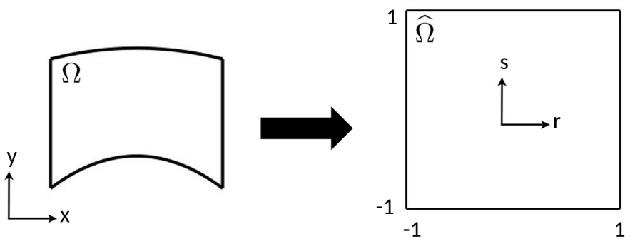
Figure 1: Schematic of mapping a physical element to a reference element.

For SEM, the 1D basis functions are chosen as the Lagrangian polynomial constructed on $P+1$ Gauss-Lobatto-Legendre (GLL) points in the reference space coordinates $r-s-t$. A Lagrangian basis defined by a quadrature rule is chosen so that the solution can be numerically integrated with only nodal evaluations and will not require interpolation [14]. The GLL points were chosen because they are the most accurate quadrature rule for polynomials that contains the end points of the element [15]. Having nodes on the element boundaries allows continuity between elements and boundary conditions to be enforced without interpolation. The basis is constructed with a tensor-product of 1D bases because the tensor-product structure can be exploited when computing derivatives and in other operations, which greatly reduces the number of floating point operations (FLOPS) for such operations [14].

In order to solve for the basis coefficients, Eqs. (5)-(6) are formulated for each individual element by substituting the local solution representation from Eq. (8) for $\bm{u}$ and $p$. This equation is satisfied for each of the local basis functions $\phi^{e}_{i}(\bm{x})$ as the test function $\bm{v}$. By doing this, an element local system of equations is formed:

$$\mathcal{M}^{e}\frac{d\underline{\bm{u}}^{e}}{dt} =\frac{1}{\rho}\mathcal{D}^{e,T}\underline{p}^{e}-\nu\mathcal{K}^{e}\underline{\bm{u}}^{e}-\mathcal{C}^{e}(\bm{u}^{e}),$$ (9)

$$\mathcal{D}^{e}\underline{\bm{u}}^{e} =0,$$ (10)

where $\mathcal{M}^{e}$ is the elemental mass matrix, $\mathcal{D}^{e}$ is the elemental differentiation matrix, $\mathcal{K}^{e}$ is the elemental stiffness matrix, $\mathcal{C}^{e}$ is the elemental non-linear convection operator, and $\underline{\bm{u}}^{e}$ is the elemental vector of coefficients $[\underline{u}_{0},\underline{u}_{1},...,\underline{u}_{N_{b}}]$. The viscosity, $\nu$, is assumed to be constant. The entries of these matrices are defined as

$$\mathcal{M}^{e}_{ij} =\int_{\Omega_{e}}{\phi_{i}^{e}\phi_{j}^{e}}\,d\Omega_{e},\qquad\mathcal{D}^{e}_{ij}=\int_{\Omega_{e}}{\frac{d\phi^{e}_{j}}{dx}\phi^{e}_{i}}\,d\Omega_{e},$$ (11)

$$\mathcal{K}^{e}_{ij} =\int_{\Omega_{e}}{\nabla\phi_{j}^{e}\cdot\nabla\phi_{i}^{e}}\,d\Omega_{e},\qquad\mathcal{C}^{e}_{j}=\int_{\Omega_{e}}{\phi^{e}_{j}\bm{u}^{e}\cdot\nabla\bm{u}^{e}}\,d\Omega_{e}.$$ (12)

Each of the entries in the matrices, as shown in Eqs. (11)-(12), are found by computing an integral over the element. These integrals are approximated using numerical quadrature. As previously mentioned, the numerical quadrature rule used in SEM is the same $P+1$ point GLL rule used to define the 1D basis functions in each direction. This quadrature rule exactly integrates polynomials of order $2P-1$. Hence, this rule is inexact for the mass matrix, because its entries are polynomials of order $2P$ [16]. However, the impact of this inexactness is minimized for higher $P$ because the error from inexact integration is of the same order as the error of the polynomial expansion [17]. The advantage of this choice of quadrature rule and basis is that each basis function is only non-zero at a single quadrature point. As a result, the basis functions have discrete orthogonality and the mass matrix is a diagonal matrix and can be easily solved. Furthermore, evaluating the solution at each quadrature point is equal to the coefficient values at the nodes and no interpolation is needed. Hence, the choice of quadrature rule and basis functions enables efficient evaluations.

One complication during the computation of the matrix terms comes when computing $\mathcal{C}^{e}$ in Eq. (12). This term comes from the non-linear convection term in the Navier-Stokes equations. Because of the non-linearity, if insufficient quadrature is used, high wavenumbers are not captured by the scheme and the energy that is supposed to be contained in those modes is aliased to lower wavenumbers, causing instability and inaccuracies in turbulent flow simulations [18]. This issue can be rectified by using a higher-order quadrature rule when computing $\mathcal{C}^{e}$, which is called overintegration or dealiasing. Because of the order of the polynomials being integrated in the term, an overintegration rule of a $1.5(P+1)$ Gauss-Legendre (GL) points is sufficient to resolve the issue [18].

Once the local system of equations is formed for each element, they are combined to form a global system of equations. SEM requires $C^{0}$ continuity between elements. To enforce this, co-located nodes are equated at each time step. These conditions are combined with the elemental systems of equations and setting nodal values on the boundary and combining equations with a direct stiffness sum to form a global system of equations for all of the local coefficients. This forms a global system of equations:

$$\mathcal{M}\frac{d\underline{\bm{u}}}{dt} =\frac{1}{\rho}\mathcal{D}^{T}\underline{p}-\nu\mathcal{K}\underline{\bm{u}}-\mathcal{C}(\bm{u}),$$ (13)

$$\mathcal{D}\underline{\bm{u}} =0,$$ (14)

where $\underline{\bm{u}}$ is the vector of global coefficients [14].

In summary, the solution procedure is to first compute the integrals in Eqs. (5)-(6) using GLL quadrature to form a local system of equations for each element. Then a direct stiffness summation is used to couple neighboring elements and to create a global system of equations to solve for the solution coefficients [19]. Finally, the equations are discretized in time and the global system of equations is solved for the basis coefficients at each time step.

The time-discretization chosen in this study is a semi-implicit BDF$k$/EXT$k$ scheme where the linear terms are treated implicitly with a $k$th-order backward difference formula and the non-linear terms are treated explicitly with a $k$th-order extrapolation [19]. The resulting discretization in time at step $t^{n}$ is

$$\sum_{j=0}^{k}\frac{\beta_{j}}{\Delta t}\mathcal{M}\underline{\bm{u}}^{n-j} =\frac{1}{\rho}\mathcal{D}^{T}\underline{p}^{n}-\nu\mathcal{K}\underline{\bm{u}}^{n}-\sum_{j=1}^{k}\alpha_{j}\mathcal{C}(\bm{u}^{n-j}),$$ (15)

$$\mathcal{D}\underline{\bm{u}}^{n} =0,$$ (16)

where $\beta_{j}$ and $\alpha_{j}$ are standard BDF$k$/EXT$k$ coefficients [19]. The scheme is accurate to $O(\Delta t^{k})$. Rearranging Eqs. (15) and (16) so that all terms at $t^{n}$ are on the left side gives

$$\frac{\beta_{0}}{\Delta t}\mathcal{M}\underline{\bm{u}}^{n}+\nu\mathcal{K}\underline{\bm{u}}^{n}-\frac{1}{\rho}\mathcal{D}^{T}\underline{p}^{n} =-\sum_{j=1}^{k}(\alpha_{j}\mathcal{C}(\bm{u}^{n-j})+\frac{\beta_{j}}{\Delta t}\mathcal{M}\underline{\bm{u}}^{n-j})$$ (17)

$$\mathcal{D}\underline{\bm{u}}^{n} =0.$$ (18)

Values of $k=1,2,3$ can be used. The implicit part of the scheme extends the stability of the scheme, while treating the non-linear term explicitly avoids having to solve a non-linear system of equations at each time step [20]. In order to reach the final solution time as quickly as possible, the timestep was adapted throughout the simulation to meet a set Courant-Friedrichs-Lewy (CFL) constraint. For notational convenience, the discrete Helmholtz matrix is defined as $\mathcal{H}=\frac{\beta_{0}}{\Delta t}\mathcal{M}+\nu\mathcal{K}$ making the overall system of equations

$$\mathcal{H}\underline{\bm{u}}^{n}-\frac{1}{\rho}\mathcal{D}^{T}\underline{p}^{n} =-\sum_{j=1}^{k}(\alpha_{j}\mathcal{C}(\bm{u}^{n-j})+\frac{\beta_{j}}{\Delta t}\mathcal{M}\underline{\bm{u}}^{n-j})$$ (19)

$$\mathcal{D}\underline{\bm{u}}^{n} =0.$$ (20)

Additionally, to improve the conditioning of the system, the change in the coefficients $\Delta\underline{\bm{u}}^{n}=\underline{\bm{u}}^{n}-\underline{\bm{u}}^{n-1}$ is solved for:

$$\mathcal{H}\Delta\underline{\bm{u}}^{n}-\frac{1}{\rho}\mathcal{D}^{T}\underline{p}^{n} =-\mathcal{H}\Delta\underline{\bm{u}}^{n-1}-\sum_{j=1}^{k}(\alpha_{j}\mathcal{C}(\bm{u}^{n-j})+\frac{\beta_{j}}{\Delta t}\mathcal{M}\underline{\bm{u}}^{n-j})$$ (21)

$$\mathcal{D}\underline{\bm{u}}^{n} =0.$$ (22)

4 Enrichment Method

The most common WMLES methods sample the solution away from the wall in the fully resolved region and apply a modeled shear stress. The modeled shear stress is applied as a slip-wall boundary condition. The solution near the wall is under resolved and serves only to pass the shear stress to the bulk. This section of the domain can contain oscillations and large amounts of slip, resulting in an unphysical section of the domain as shown in Fig. 2. The unphysical section in the domain can cause inaccuracies when computing wall quantities and coupling physics in the near-wall region, such as Lagrangian particles which are very sensitive to the flow and geometry near the wall [21]. To address these issues, we developed a solution enrichment based wall-model. Instead of modifying the boundary conditions at the wall, we modify the solution representation to capture the modeled boundary layer profile without unphysical oscillations due to under-resolution.

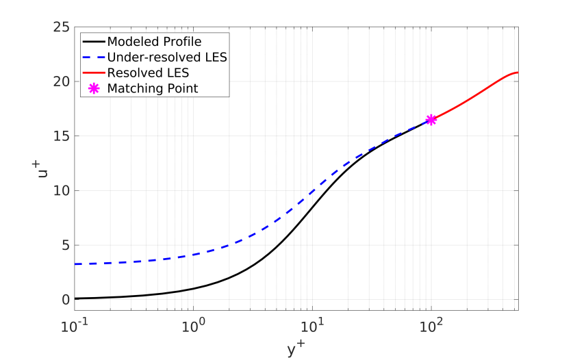
Figure 2: Schematic of the shear stress wall-model showing the under-resolved region near the wall and the resolved region connected by the matching point

The overall idea is that in a subset of the domain, $\Omega_{\psi}$, the polynomial solution is enriched with an enrichment function $\bm{\psi}(\bm{x},t)$. This function represents a feature in the solution that cannot be accurately captured by the polynomial basis. Typically such features are non-polynomial functions with too large of gradients to capture with the polynomial basis without unphysical oscillations. For this application, the enrichment function will capture the mean velocity profile of the turbulent boundary layer and will be discussed in detail in Section 5. The enriched solution representation is:

$$\bm{u}(\bm{x},t)=\bm{u_{p}}(\bm{x},t)+\bm{\psi}(\bm{x},t),$$ (23)

where $\bm{u_{p}}$ is the polynomial component of the solution defined on the standard SEM basis:

$$\bm{u_{p}}=\sum_{i}^{N_{b}}\underline{\bm{u}}_{i}\phi_{i}(\bm{x}).$$ (24)

With this representation, the enrichment function is able to capture the difficult flow feature and the polynomials can capture other features or fluctuations.

To further develop the method, the enriched solution representation is substituted into the weighted residual form in Eqs. 5-6:

$$\frac{\partial}{\partial t}(\bm{v},\bm{u_{p}}+\bm{\psi})= (\nabla\bm{v},p)-(\nabla\bm{v},\left[\nu\left(\nabla(\bm{u_{p}}+\bm{\psi})+\nabla(\bm{u_{p}}+\bm{\psi})^{T}\right)\right])$$ (25)

$$-(\bm{v},(\bm{u_{p}}+\bm{\psi})\cdot\nabla(\bm{u_{p}}+\bm{\psi})),$$

$$(\nabla\cdot(\bm{u_{p}}+\bm{\psi}),q)= \,0.$$ (26)

Then equations are algebraically manipulated to separate the enrichment terms from the polynomial terms:

$$\frac{\partial}{\partial t}(\bm{v},\bm{u_{p}}) =(\nabla\cdot\bm{v},p)-(\nabla\bm{v},\nu(\nabla\bm{u_{p}}+\nabla\bm{u_{p}}^{T}))-(\bm{v},\bm{u_{p}}\cdot\nabla\bm{u_{p}})$$ (27)

$$-(\nabla\bm{v},\nu\left(\nabla\bm{\psi}+\nabla\bm{\psi}^{T}\right))-(\bm{v},\bm{u_{p}}\cdot\nabla\bm{\psi})-(\bm{v},\bm{\psi}\cdot\nabla\bm{u_{p}})$$

$$-(\bm{v},\bm{\psi}\cdot\nabla\bm{\psi})-\frac{d}{dt}(\bm{v},\bm{\psi}),$$

$$(\nabla\cdot\bm{u_{p}},q)+ (\nabla\cdot\bm{\psi},q)=0.$$ (28)

For the application to WMLES, we assume the enrichment function is adapted between timesteps using the wall-parallel velocity component at matching points. Hence, the time derivative of the enrichment function is put to the right hand side of Eq. (27). With the governing equations in this form, the left-hand side and the first three terms on the right-hand side are the same as in the traditional SEM and the last five terms on the right-hand side are additions from the enrichment [22]. This separability shows that the presented enrichment method can be implemented with the addition of associated terms into an existing solver for ease of implementation.

To fully define these terms, the local systems of equations are formed by substituting in the local solution representation and letting the test function be the local basis functions, $\phi_{i}^{e}(\bm{x})$. Through this the local system of equations is formed:

$$\mathcal{M}^{e}\frac{d\underline{\bm{u}}^{e}_{p}}{dt} =\frac{1}{\rho}\mathcal{D}^{e,T}\underline{p}^{e}-\nu\mathcal{K}^{e}\underline{\bm{u}}^{e}_{p}-\mathcal{C}^{e}(\bm{u}^{e}_{p})-\mathcal{V}^{e}_{\psi}-\mathcal{C}^{e}_{\psi}(\bm{u}^{e}_{p})-\frac{d}{dt}(\mathcal{M}^{e}_{\psi}),$$ (29)

$$\mathcal{D}^{e}\underline{\bm{u}}^{e}+\mathcal{D}^{e}_{\psi} =0,$$ (30)

where $\mathcal{V}_{\psi}$ is the viscous enrichment operator, $\mathcal{C}_{\psi}$ is the convective enrichment operator, $\mathcal{D}_{\psi}$ is differentiation enrichment operator, and $\mathcal{M}_{\psi}$ is the enrichment mass operator. The entries of these matrices are defined as

$$\mathcal{V}^{e}_{\psi,j} =\int_{\Omega_{e}}{\nu\nabla\phi_{j}^{e}\cdot(\nabla\bm{\psi}^{e}+\nabla\bm{\psi}^{e,T})}\,d\Omega_{e},\qquad\mathcal{D}^{e}_{\psi,j}=\int_{\Omega_{e}}{\nabla\cdot\bm{\psi}^{e}\phi^{e}_{j}}\,d\Omega_{e},$$ (31)

$$\mathcal{C}^{e}_{\psi,j}(\bm{u}^{e}_{p}) =\int_{\Omega_{e}}{\phi_{j}^{e}(\bm{u}^{e}_{p}\cdot\nabla\bm{\psi}^{e}+\bm{\psi}^{e}\cdot\nabla\bm{u}^{e}_{p}+\bm{\psi}^{e}\cdot\nabla\bm{\psi}^{e})}\,d\Omega_{e},$$ (32)

$$\mathcal{M}^{e}_{\psi,j} =\int_{\Omega_{e}}{\phi_{j}^{e}\bm{\psi}^{e}}\,d\Omega_{e}.$$ (33)

As with the standard SEM matrix entries, these are computed with numerical quadrature over the elements. However, the enrichment function contains a feature that the polynomial basis cannot resolve. Hence, quadrature rules designed for order $P$ polynomials, like the standard $P+1$ point GLL quadrature rule, are likely to be inaccurate when integrating the enrichment function. To address this issue, a quadrature rule designed for the enrichment function is used. If it can be integrated exactly or accurately with a specific quadrature rule, that should be used. If the enrichment function’s structure cannot be exploited, we have found using a higher-order GL or GLL quadrature rule to be sufficient for smooth functions. Numerical accuracy tests are performed to determine a heuristic for a particular enrichment function and basis order.

As before, Eqs. (29)-(30) are discretized in time using the BDF$k$/EXT$k$ scheme where the viscous terms are treated implicitly and the convective terms are treated explicitly:

$$\sum_{j=0}^{k}\frac{\beta_{j}}{\Delta t}\mathcal{M}\underline{\bm{u}}^{n-j}_{p}= \frac{1}{\rho}\mathcal{D}^{T}\underline{p}^{n}-\nu\mathcal{K}\underline{\bm{u}}^{n}_{p}-\sum_{j=1}^{k}\alpha_{j}\mathcal{C}(\bm{u}^{n-j}_{p})$$ (34)

$$-\mathcal{V}_{\psi}^{n}-\sum_{j=1}^{k}\alpha_{j}\mathcal{C}^{n-j}_{\psi}(\bm{u}_{p}^{n-j})-\sum_{j=0}^{k}\frac{\beta_{j}}{\Delta t}\mathcal{M}_{\psi}^{n-j},$$

$$\mathcal{D}\underline{\bm{u}}^{n}+\mathcal{D}_{\psi}= 0.$$ (35)

Rearranging the equations to group the variables being solved for gives:

$$\mathcal{H}\underline{\bm{u}}^{n}_{p}-\frac{1}{\rho}\mathcal{D}^{T}\underline{p}^{n} =-\sum_{j=1}^{k}\left(\alpha_{j}\mathcal{C}(\bm{u}^{n-j}_{p})+\frac{\beta_{j}}{\Delta t}\mathcal{M}\underline{\bm{u}}^{n-j}_{p}\right)$$ (36)

$$-\sum_{j=1}^{k}\left(\alpha_{j}\mathcal{C}_{\psi}^{n-j}(\bm{u}^{n-j}_{p})+\frac{\beta_{j}}{\Delta t}\mathcal{M}_{\psi}^{n-j}\right)-\left(\frac{\beta_{0}}{\Delta t}\mathcal{M}^{n}_{\psi}+\mathcal{V}^{n}_{\psi}\right)$$

$$\mathcal{D}\underline{\bm{u}}^{n}+\mathcal{D}_{\psi}= 0.$$ (37)

In matrix form, as well as variational form, the enrichment terms can be separated from the standard SEM terms. Finally, the equations are modified to solve for the change in the coefficients:

$$\mathcal{H}\Delta\underline{\bm{u}}^{n}_{p}-\frac{1}{\rho}\mathcal{D}^{T}\Delta\underline{p}^{n} =-\mathcal{H}\Delta\underline{\bm{u}}^{n-1}_{p}+\frac{1}{\rho}\mathcal{D}^{T}\Delta\underline{p}^{n-1}$$ (38)

$$-\sum_{j=1}^{k}\left(\alpha_{j}\mathcal{C}(\bm{u}^{n-j}_{p})+\frac{\beta_{j}}{\Delta t}\mathcal{M}\underline{\bm{u}}^{n-j}_{p}\right)$$

$$-\sum_{j=1}^{k}\left(\alpha_{j}\mathcal{C}_{\psi}^{n-j}(\bm{u}^{n-j}_{p})+\frac{\beta_{j}}{\Delta t}\mathcal{M}_{\psi}^{n-j}\right)-\left(\frac{\beta_{0}}{\Delta t}\mathcal{M}^{n}_{\psi}+\mathcal{V}^{n}_{\psi}\right)$$

$$\mathcal{D}\Delta\underline{\bm{u}}^{n}+\mathcal{D}_{\psi}= -\mathcal{D}\underline{\bm{u}}^{n-1}.$$ (39)

Solving for the change in polynomial coefficients at each timestep ensure that the solution remains continuous across elements with different enrichment values.

The solution procedure for the polynomial coefficients is exactly the same as the standard SEM and high-order polynomial portion of the solution representation is maintained. Hence, the addition of the enrichment function improves the method’s ability to capture the targeted flow feature without affecting the high-order accuracy.

5 Enrichment Function

For the presented wall-model, the enrichment function is designed to capture the mean velocity profile in a turbulent boundary layer. The enrichment function models the large gradients of this profile without oscillations or modified boundary conditions. This leaves the polynomial part of the solution to represent the turbulent fluctuations.

In order to fit the enrichment function to the local flow, like in shear stress wall-models, a set of matching points off the wall are selected in the resolved LES region. The wall-parallel velocity at these points is fed to a law-of-the-wall function to form the enrichment function. We take the matching points to be at the far end of the wall-adjacent elements because it is assumed that the entire law-of-the-wall profile is contained in the first element. In other studies, this choice has been shown to prevent log-layer mismatch [6].

The wall-parallel velocity, $u_{\|}$, and the distance from the wall, $h_{w}$, at the matching points are fed to a law-of-the-wall function, $f_{w}(h_{w},u_{\tau})$ and the implicit nonlinear equation is solved for the friction velocity, $u_{\tau}$:

$$u_{\|}=f_{w}(h_{w}(\bm{x}),u_{\tau}).$$ (40)

Any algebraic law-of-the-wall function would fit into the method. In this study, we use the Reichardt law-of-the-wall due to its popularity in WMLES methods, its smoothness, and its ease of computation:

$$f_{w}(h_{w}(\bm{x}),u_{\tau})=u_{\tau}\left(\frac{1}{0.41}\log(1+0.41y^{+})+7.8(1-e^{-\frac{y^{+}}{11}}-\frac{y^{+}}{11}e^{-\frac{y^{+}}{3}})\right),$$ (41)

where $y^{+}=h_{w}u_{\tau}/\nu$ is the non-dimensional plus distance from the wall.

The nodes on the wall are indexed from $1$ to $P+1$ as $i$ and $j$ for the $r$ and $t$ reference space directions, respectively. For each node on the wall, the matching point is defined to be the location of the corresponding node on the opposite side of the element. The value of $u_{\tau}$ for each node $(i,j)$ is computed using Eq. 40 and is notated $u_{\tau,(i,j)}$. Once a value for $u_{\tau,(i,j)}$ is computed for each matching point $(i,j)$, the law-of-the-wall enrichment function is constructed. In order to capture the law-of-the-wall profile in the wall normal direction, at each node, the enrichment function is defined using the same law-of-the-wall function in the wall-normal direction and polynomials:

$$\bm{\psi}^{e}_{(i,j)}(\bm{x})=f_{w}(h_{w}(\bm{x}),u^{e}_{\tau,(i,j)})\hat{\bm{t}}^{e}_{w,(i,j)}(\bm{x}),$$ (42)

where $e$ is the element wherein the enrichment function is defined, $\hat{\bm{t}}_{w,(i,i)}(\bm{x})$ is the unit tangent vector to the wall at node $(i,j)$ [22]. The wall-normal profiles are connected to form a continuous and smooth enrichment function using a standard $P+1$ order nodal basis in the wall-parallel directions. The resulting enrichment function in element $e$ is

$$\bm{\psi}_{w}^{e}(\bm{x})= \sum_{i=1}^{P+1}\sum_{j=1}^{P+1}\bm{\psi}^{e}_{(i,j)}(\bm{x})\phi^{e}_{i}(r)\phi^{e}_{j}(t),$$ (43)

$$= \sum_{i=1}^{P+1}\sum_{j=1}^{P+1}f_{w}(h_{w}(\bm{x}),u^{e}_{\tau,(i,j)})\hat{\bm{t}}^{e}_{w,(i,j)}(\bm{x})\phi^{e}_{i}(r)\phi^{e}_{j}(t),$$ (44)

where $r$ and $t$ are defined as the wall-parallel directions and $\phi_{i}$ is the $i$th 1D nodal GLL basis function. The enriched domain, $\Omega_{\psi}$, is defined as only the wall-adjacent elements because the matching locations are chosen to be at the upper end of the wall-adjacent elements.

The enrichment function is evolved in time to match local flow features at each timestep or at a set frequency. After the polynomial solution is computed at a timestep using Eqs. (36)-(37), a new enrichment function can be computed as described earlier. Then an $L_{2}$ projection is used to compute the new polynomial coefficients. From experimentation, it was seen that time-averaged velocities over a flow-through time tended to be more stable than instantaneous values, so they will be used going forward. This time evolution strategy is consistent with the WMLES literature where the instantaneous and time-averaged matching velocity values have similar errors [3].

In order to accurately compute the integrals in Eqs. (31)-(33) a quadrature must be tailored for the enrichment function. The enrichment wall-model is a continuous and smooth function with no exploitable structure. Hence, simple overintegration is used. From testing, we determined that overintegrating using $1.5(P+1)$ GL quadrature points was sufficient to accurately resolve the integrals for a range of polynomial orders and Reynolds numbers.

The resulting algorithm to compute the enrichment function is detailed in Algorithm 1. This wall-model takes the matching point sufficiently far from the wall to prevent log-layer mismatch while the enrichment formulation ensures that the large gradients are captured in the solution without unphysical oscillations or unphysical boundary conditions.

Algorithm 1 Computing Enrichment Algorithm

for each element on the wall do

     for each node $(i,j)$ on the wall do

         Sample $u_{\|}$ and $h_{w}$ on the opposite end of the element.

         Solve for $u_{\tau}$ with Eq. (40).

         Compute $\bm{\psi}$ with Eq. (44).

     end for

     Project onto solution with new enrichment function

end for

6 Numerical Results

The main test case considered for demonstration studies in the present work is the turbulent channel flow. The case is set up in non-dimensional form by choosing a domain of size $[2\pi h,2h,\pi h]$ where $h$ is the half-height of the channel. The domain size ensures flow decorrelation of the turbulent structures. Periodic boundary conditions are used in the $x$ and $z$ directions. No-slip wall boundary conditions are used in the $y$ direction. In order to ensure that the flow in the channel is maintained, a variable forcing function that ensures a constant mass flow throughout the domain is applied [23]. The mass flow rate and domain are fixed, so only $\nu$ is changed to set $Re_{\tau}$.

In order for the turbulent flow to become fully developed and statistically stationary, the flow is initialized with perturbations to speed the transition to turbulence. The initial conditions used in this work are

$$u= Re_{\tau}\left(\frac{1}{k}\log{(1+ky^{+})}+(C-\frac{1}{k}\log{k})(1-e^{-\frac{y^{+}}{11}}-\frac{y^{+}}{11}e^{-\frac{y^{+}}{3}}\right)$$ (45)

$$+\epsilon\beta\sin(\alpha x)\cos(\beta z),$$

$$v= \epsilon\sin(\alpha x)\cos(\beta z),$$ (46)

$$w= -\epsilon\alpha\cos(\alpha x)\sin(\beta z),$$ (47)

where $Re_{\tau}$ is the target friction Reynolds number, $C=5.17$ and $k=0.41$ are constants from the Reichardt law-of-the-wall, $\epsilon$ is the magnitude of the perturbation, and $\alpha$ and $\beta$ are the frequencies of the perturbations. For this study, values of $\epsilon=10^{-2}$, $\alpha=23$, and $\beta=13$ were used, so that turbulence tripped in the first flow-through time. Additionally, with a channel half-height of $h=1$, a constant mass flow rate of $\dot{m}=1$ was used. The Reynolds numbers targeted in this work are $Re_{\tau}=543,1000,2000,5200$ which have corresponding viscosities of $\nu=10^{-4},5\times 10^{-5},2.5\times 10^{-5},8\times 10^{-6}$ and these conditions match those used by Lee et al. [24].

The simulation is allowed to develop for 8 flow-through times and then statistics are computed for 300 flow-through times. The wall-model is turned on after 8 flow-through times and thereafter the flow is allowed to fully develop. For the enriched wall-model, the wall-parallel velocity used at the matching point is chosen to be the local time-averaged value over the last 50 time units, which corresponds to approximately 8 flow-through times. The Reichardt law-of-the-wall is used as the wall function in the enrichment function. The meshes used are meshes with $N$ uniform elements in each direction to ensure that they remain coarse in the near-wall region.

6.1 Grid Resolution Study

The enriched wall-model was tested on a number of coarse mesh resolutions, polynomial order, and Reynolds numbers. These cases will show the generalizability of the wall-model and test its performance for challenging high Reynolds number conditions with larger gradients captured by the enrichment function.

Figures 3 and 4 show the mean velocity profiles for turbulent channel flows with $Re_{\tau}=543$, $1000$, and $2000$ with $N=10$ and $N=20$ elements respectively. The results are shown for bases of order $P=5$, $6$, and $7$. The mean profiles are shifted up by $4$ for visibility as the Reynolds number is increased. For all of the cases, the mean velocity profile is in good agreement with the DNS data wall the way up to the wall. There is no mismatch in the near-wall region because the no-slip boundary is enforced. The $Re_{\tau}=2000$ with $N=10$ shows some log layer mismatch, but as $N$ is increased to $20$, good agreement is seen. As expected, better agreement with the DNS data is seen for the lower Reynolds number cases and cases with better resolution, but good agreement is seen throughout.

Figures 5 and 6 show the rms quantities for these cases with offsets for visibility. The rms data show similar trends to the DNS data. For the more underresolved cases in terms of polynomial order and Reynolds number, the rms values are underpredicted. However, as $P$ and $N$ are increased, better agreement is seen. In the more under-resolved cases, peaks in the rms data can be seen at the end of the first element. For example, for $Re_{\tau}=2000$, data peaks can be seen at $y^{+}=200$. This location corresponds with the end of the wall-adjacent element, which is the matching point location. This behavior is seen in under-resolved SEM simulations due the discontinuous gradient at this location, because only $C^{0}$ continuity is enforced at element boundaries [25] [26]. It is a sign of an under-resolved mesh [25], which is expected because the large wall-adjacent element motivates the need for the wall model. Despite this inaccuracy in the gradients, good agreement in the mean velocity profile is seen, highlighting the strength of the enrichment wall-model. Additionally, Figures 5 and 6 show that this can be remedied with increased resolution, like increasing $P$.

Table 1 lists the size of the wall-adjacent element and the computed friction velocity for the channel flow tests with $Re_{\tau}=543$, $1000$, and $2000$. The wall-adjacent elements are hundreds of plus units long and extend well into the bulk of the flow. The enrichment wall-model enables the use of these very large elements and still agrees well with the DNS. Additionally, the computed friction Reynolds numbers show good agreement with the DNS data with errors under 1%. Hence, the WMLES results are modeling the correct flow behavior. Additionally, the error in the friction velocity decreases as $N$ and $P$ increase.

For all three $Re_{\tau}$ values, increasing $P$ improves the mean velocity, rms quantities, and the computed $u_{\tau}$. This shows that the model still allows the solution to converge with increasing resolution as it would in the traditional SEM. Table 1 shows that large elements are being used near the wall in all cases. For all three Reynolds numbers, resolutions with the first element around $y_{1}^{+}=200$ show good agreement with the mean but under-predicted rms quantities. However, for $y_{1}^{+}\leq 100$ both the mean and rms quantities show good agreement with the DNS data. While both lead to convergence, changing the size of the elements leads to more improvement, especially for the turbulent fluctuations. Increasing the Reynolds number requires additional refinement of $N$ or $P$ because of the larger gradients in the boundary layer profile.

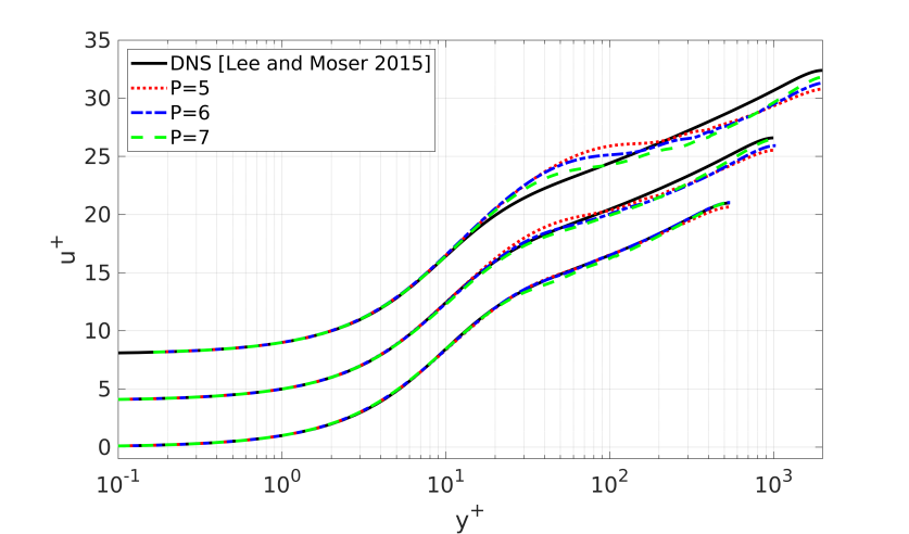
Figure 3: Mean velocity from WMLES of turbulent channel with $P=5,6,7$ order basis polynomials. Results for $Re_{\tau}=543$, $N=10$, $Re_{\tau}=1000$, $N=10$, and $Re_{\tau}=2000$, $N=10$ are shown from bottom to top, shifted up by 4 for visibility. The solutions uses a law-of-the-wall enrichment function in the wall-adjacent elements as the wall-model. The results are compared with the DNS data from [24].

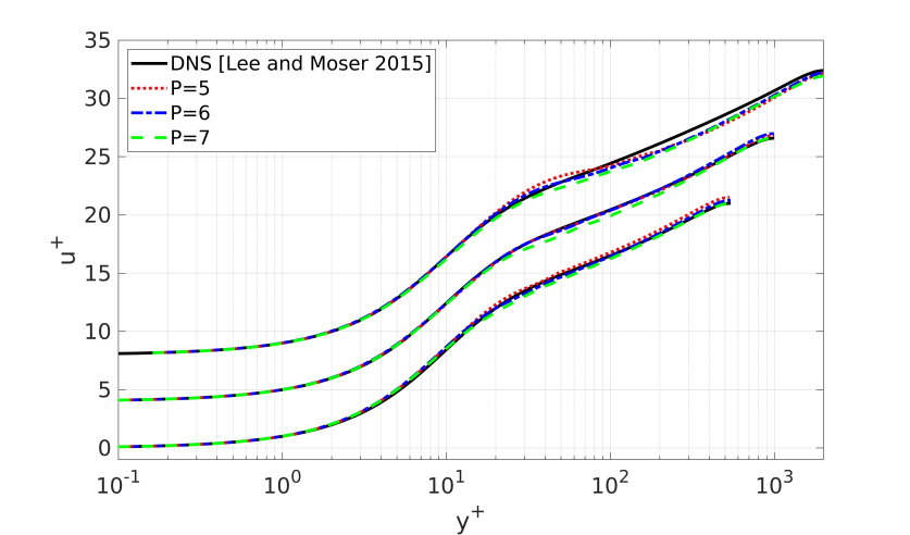
Figure 4: Mean velocity from WMLES of turbulent channel with $P=5,6,7$ order basis polynomials. Results for $Re_{\tau}=543$, $N=20$, $Re_{\tau}=1000$, $N=20$, and $Re_{\tau}=2000$, $N=20$ are shown from bottom to top, shifted up by 4 for visibility. The solutions uses a law-of-the-wall enrichment function in the wall-adjacent elements as the wall-model. The results are compared with the DNS data from [24].

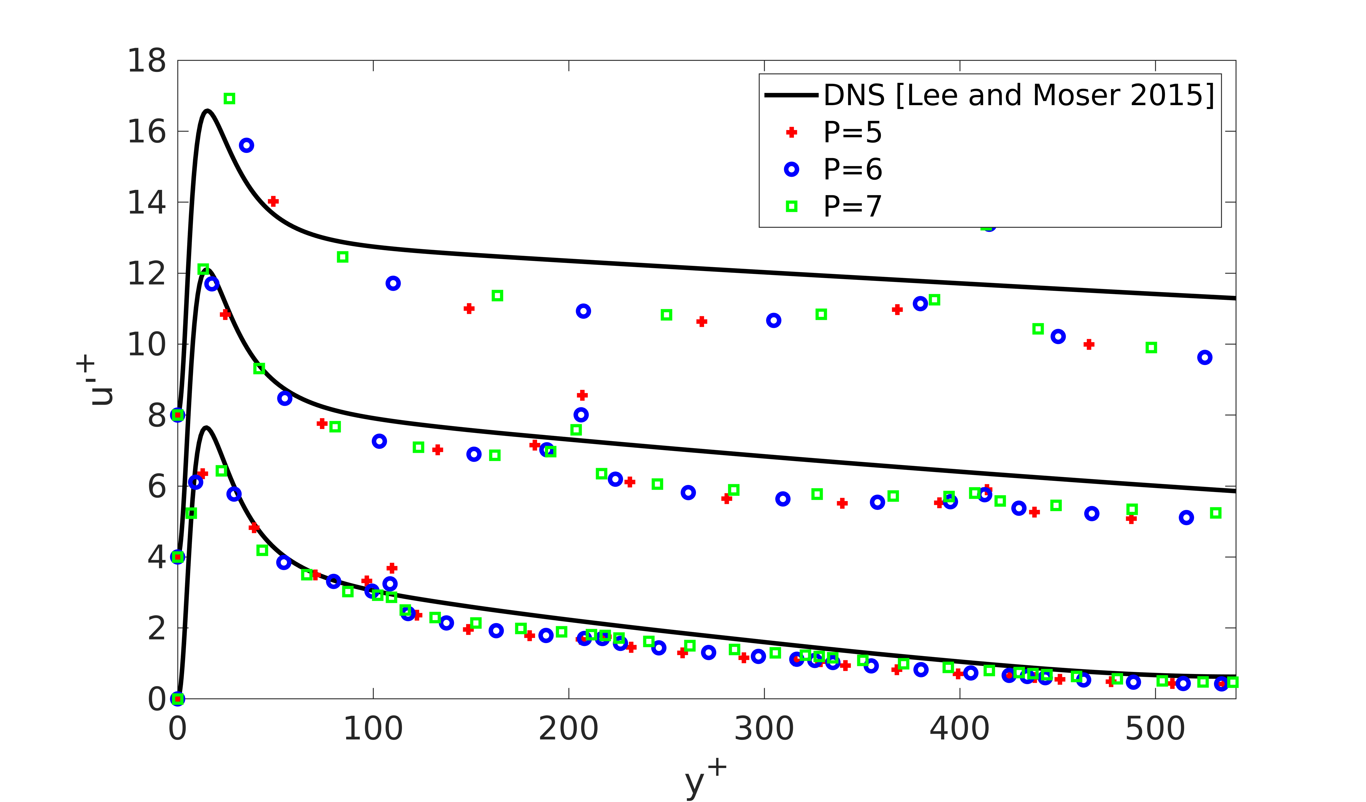
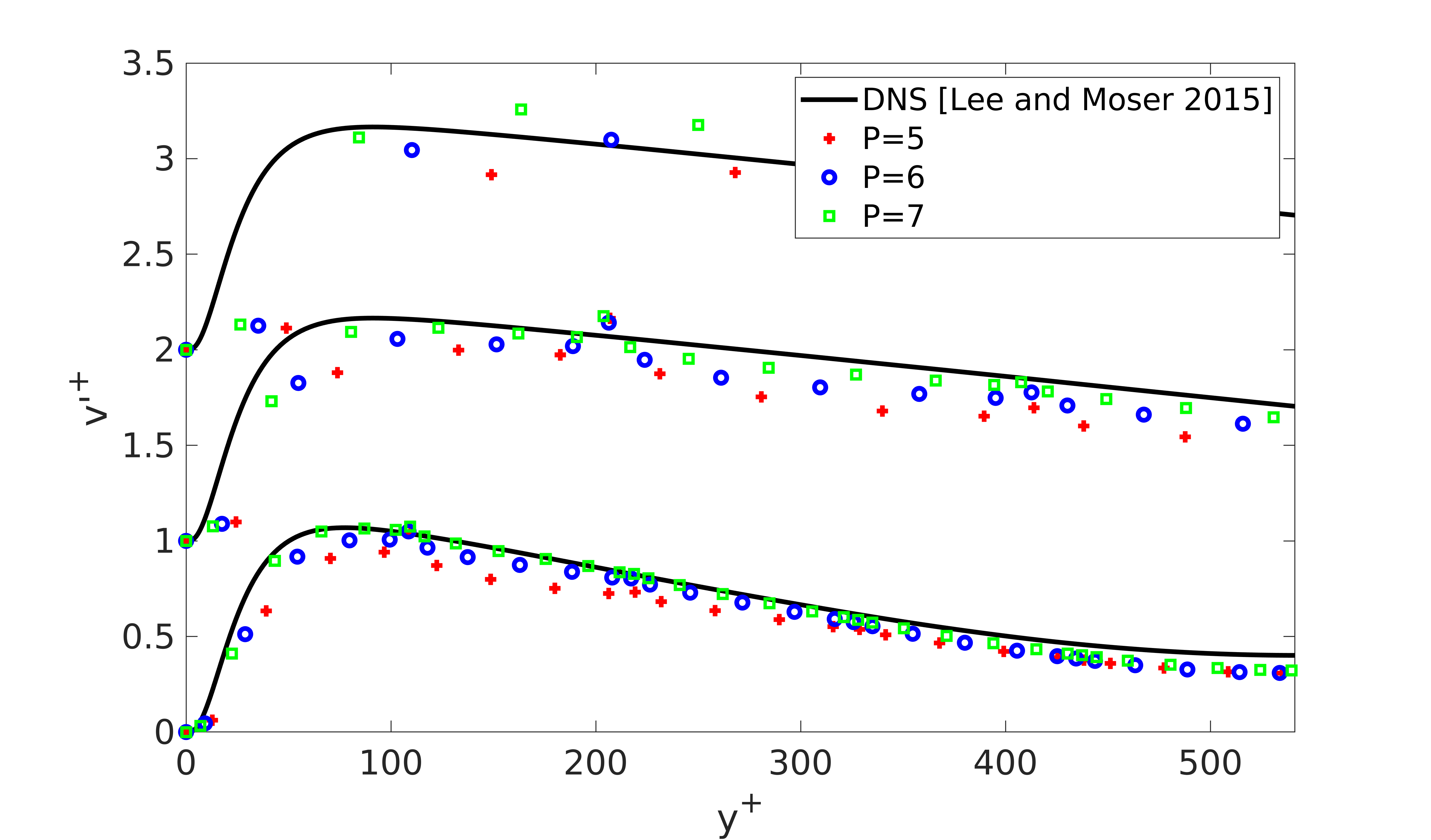
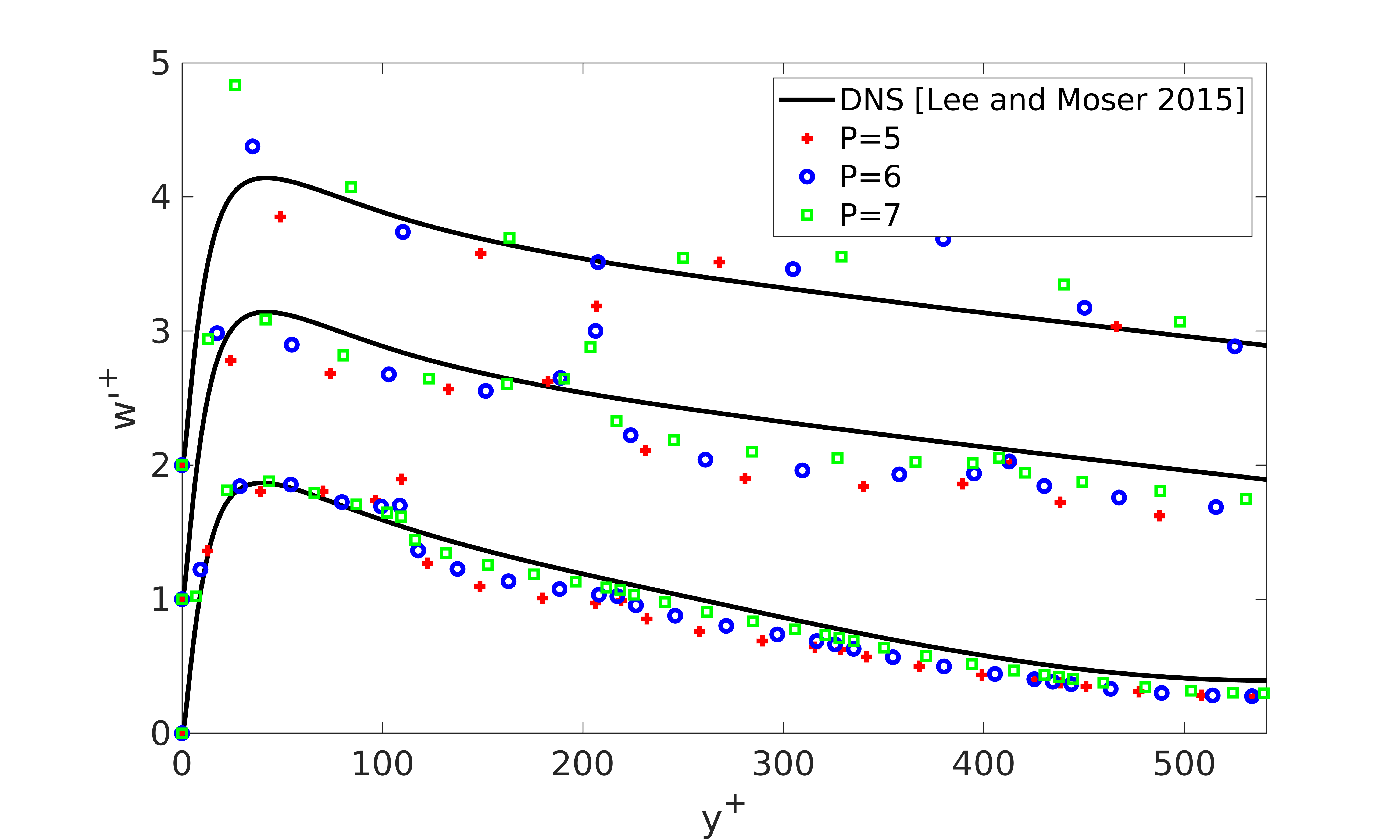
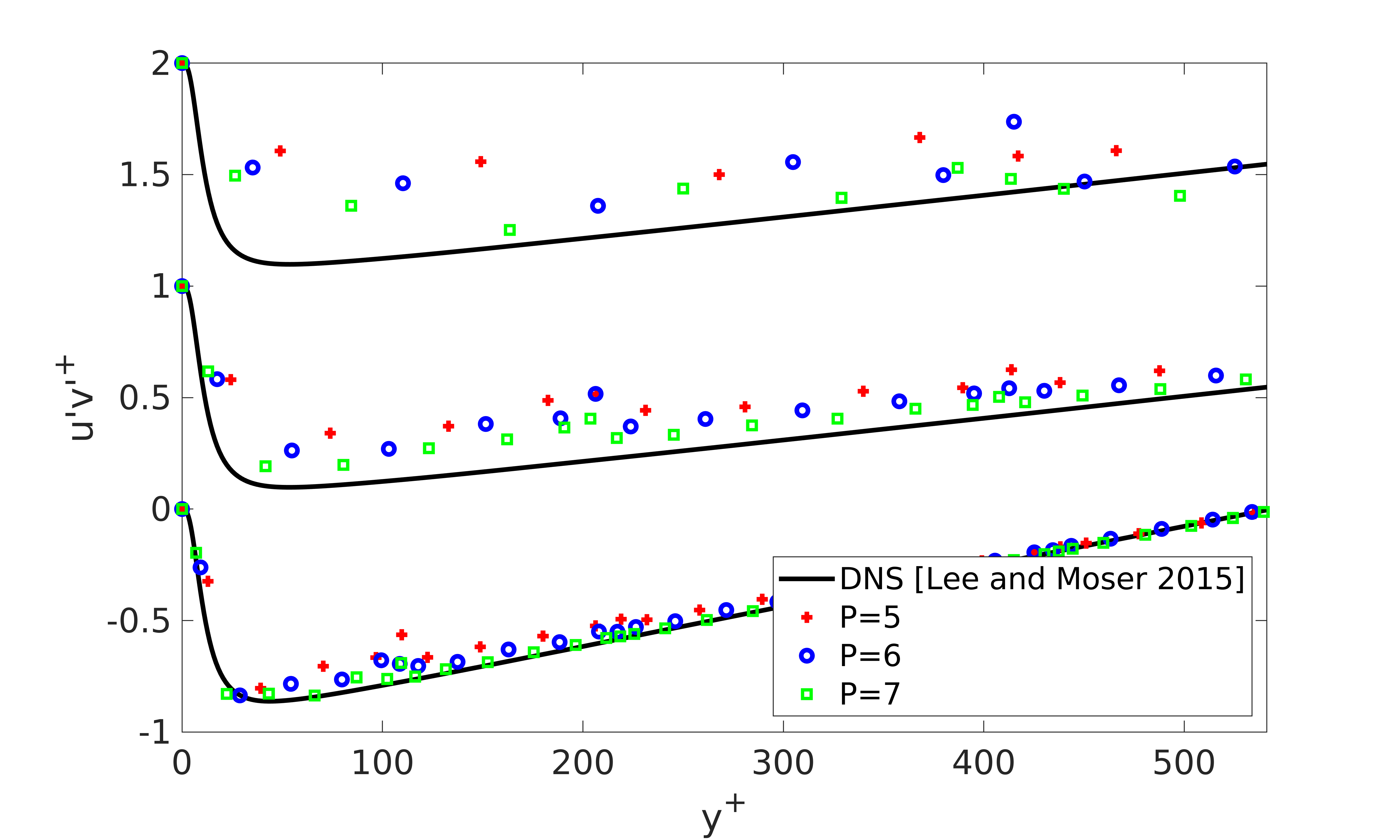
Figure 5: Rms from WMLES of turbulent channel with $P=5,6,7$ order basis polynomials. Results for $Re_{\tau}=543$, $N=10$, $Re_{\tau}=1000$, $N=10$, and $Re_{\tau}=2000$, $N=10$ are shown from bottom to top, shifted up by 4 for $u^{\prime+}$ and 1 for the other quantities for visibility. The solutions uses a law-of-the-wall enrichment function in the wall-adjacent elements as the wall-model. The results are compared with the DNS data from [24]. The results are compared with the DNS data from [24].

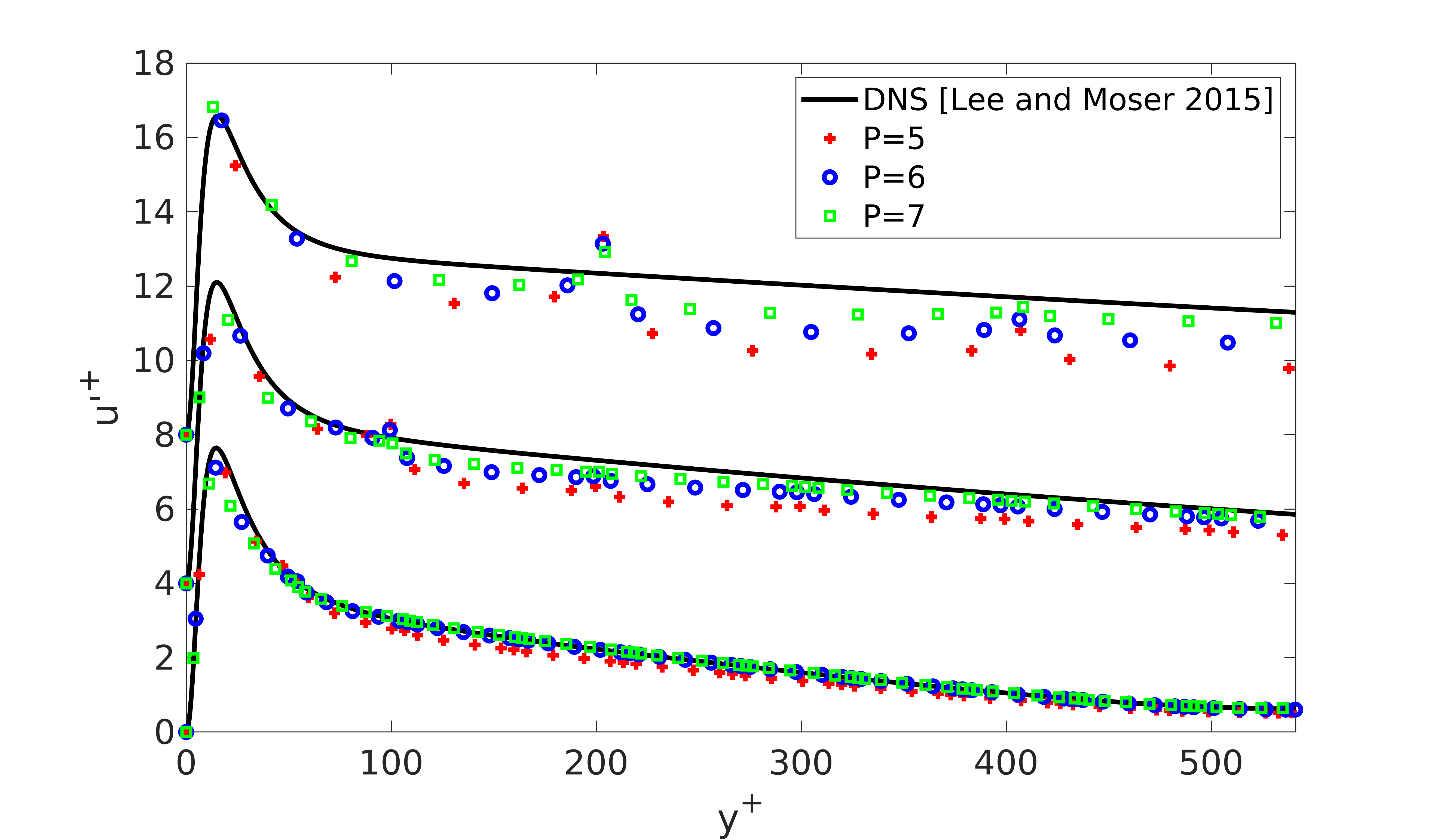
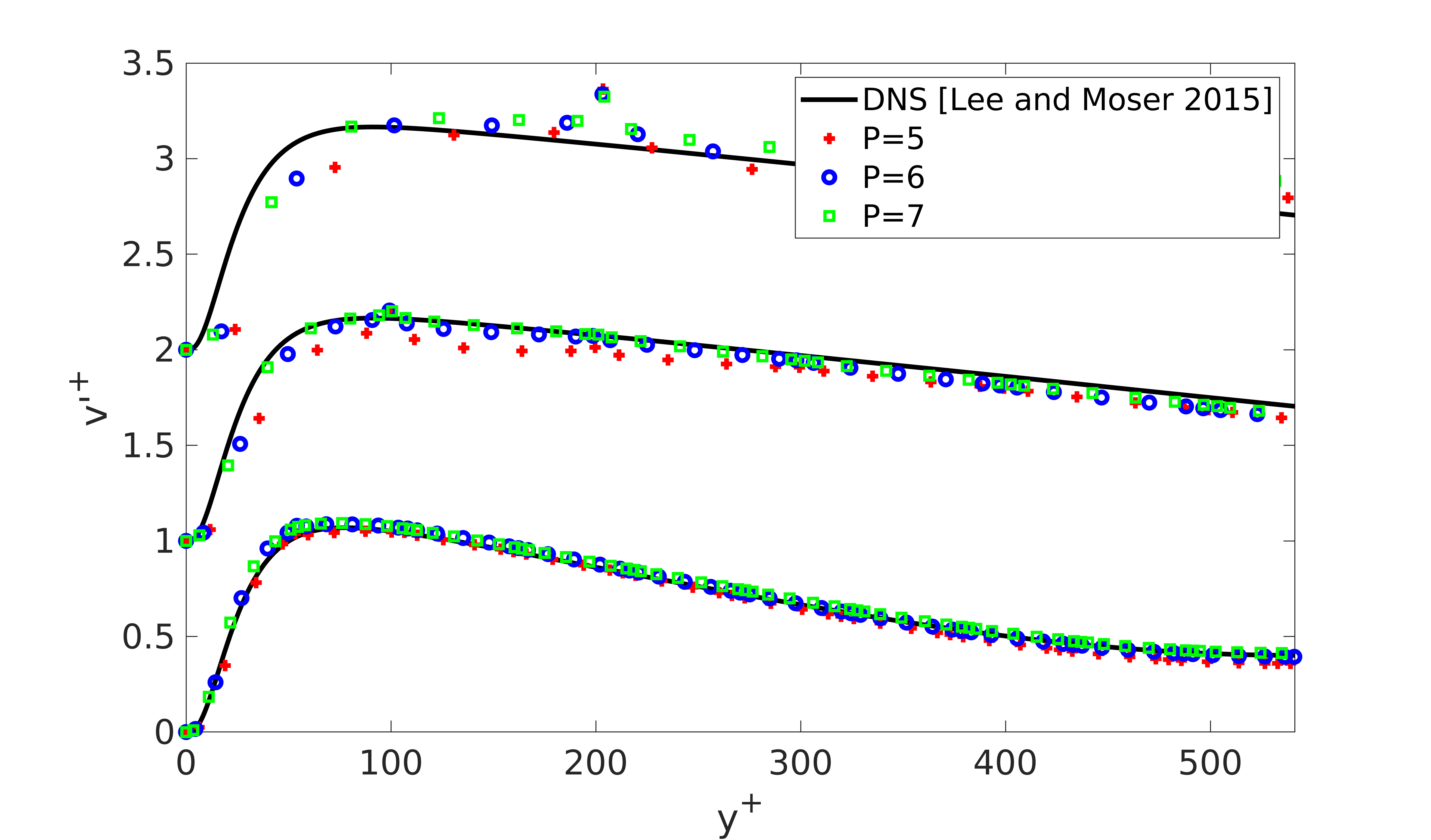
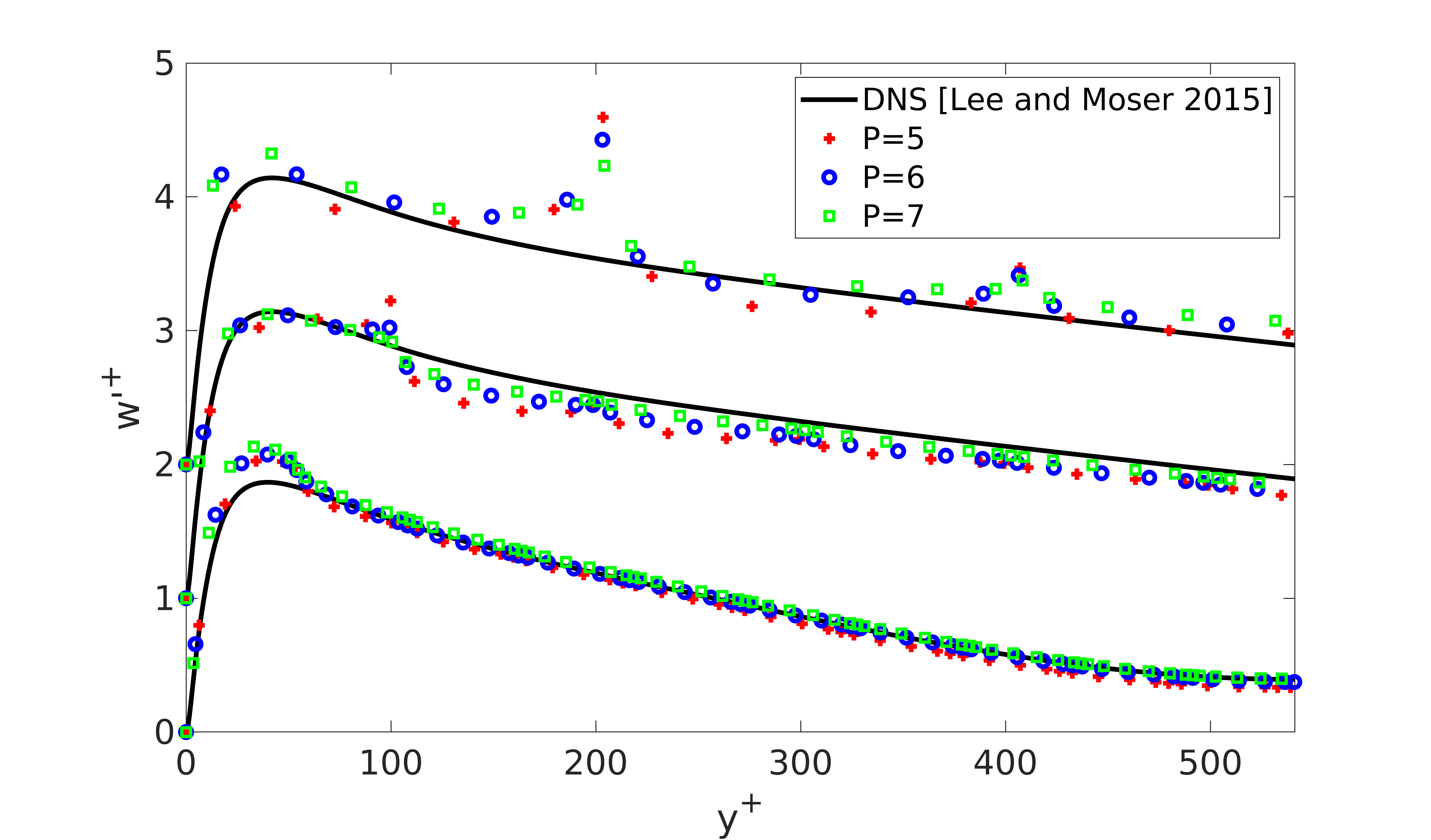
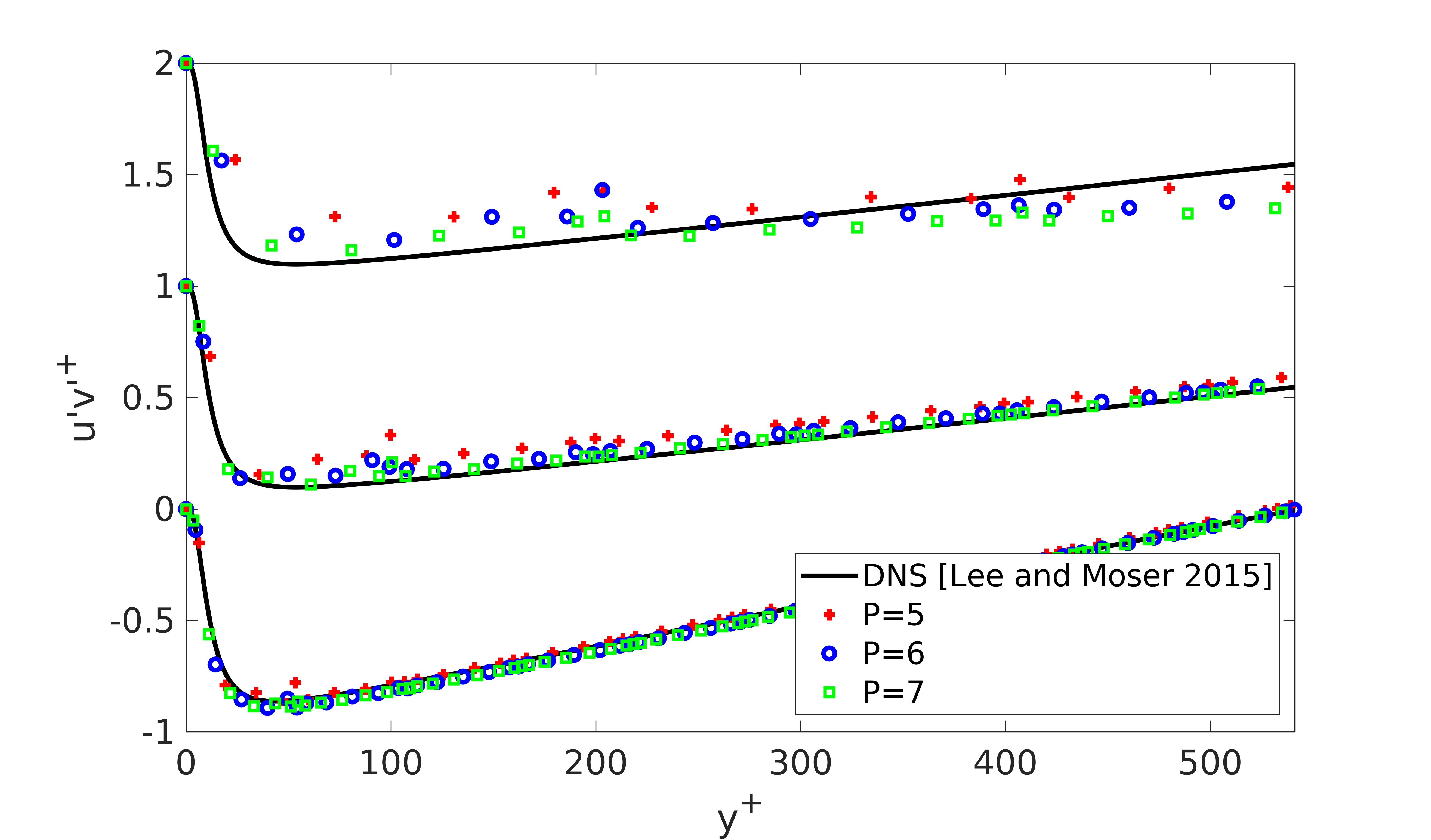
Figure 6: Rms from WMLES of turbulent channel with $P=5,6,7$ order basis polynomials. Results for $Re_{\tau}=543$, $N=20$, $Re_{\tau}=1000$, $N=20$, and $Re_{\tau}=2000$, $N=20$ are shown from bottom to top, shifted up by 4 for $u^{\prime+}$ and 1 for the other quantities for visibility. The solutions uses a law-of-the-wall enrichment function in the wall-adjacent elements as the wall-model. The results are compared with the DNS data from [24]. The results are compared with the DNS data from [24].

	$Re_{\tau}=543$		$Re_{\tau}=1000$		$Re_{\tau}=2000$
Case	$y_{1}^{+}$	$u_{\tau}$	$y_{1}^{+}$	$u_{\tau}$	$y_{1}^{+}$	$u_{\tau}$
DNS [24]	-	0.0543	-	0.0500	-	0.0459
N=10 P=5	109.55	0.0548	206.89	0.0517	417.06	0.0480
N=10 P=6	108.60	0.0543	206.32	0.0516	415.02	0.0477
N=10 P=7	109.33	0.0547	203.77	0.0509	413.46	0.0475
N=20 P=5	54.28	0.0533	99.80	0.0499	203.51	0.0468
N=20 P=6	54.09	0.0541	99.30	0.0496	203.20	0.0467
N=20 P=7	54.60	0.0546	100.63	0.0503	204.09	0.0469

Table 1: Friction velocity, $u_{\tau}$, and wall-adjacent element size, $y_{1}^{+}$, for WMLES with the enrichment wall-model.

6.2 Separation of Mean and Fluctuations

One of the attractive properties of the enrichment wall-model is the separation of the mean and fluctuations in the solution representation. The enrichment function is designed to capture the mean behavior, while the polynomial component captures the turbulent fluctuations. Figure 7 shows the mean velocity from the $Re_{\tau}=543$, $P=5$, $N=10$ and $Re_{\tau}=1000$, $P=5$, $N=20$ cases broken up into the enrichment and polynomial components. The vertical line in the plot corresponds to the edge of the first element because it is where the enrichment component becomes zero. The enrichment function contains the large gradients in the wall-adjacent element as expected. The mean of the polynomial component in the enriched portion of the domain is close to zero, as is expected because it captures the fluctuations around the mean. The mean polynomial solution is not exactly zero, because the enrichment function contains the modeled mean velocity profile near the wall and not the true mean profile. Overall, the enrichment method delivers the desired separation between mean and turbulent fluctuations.

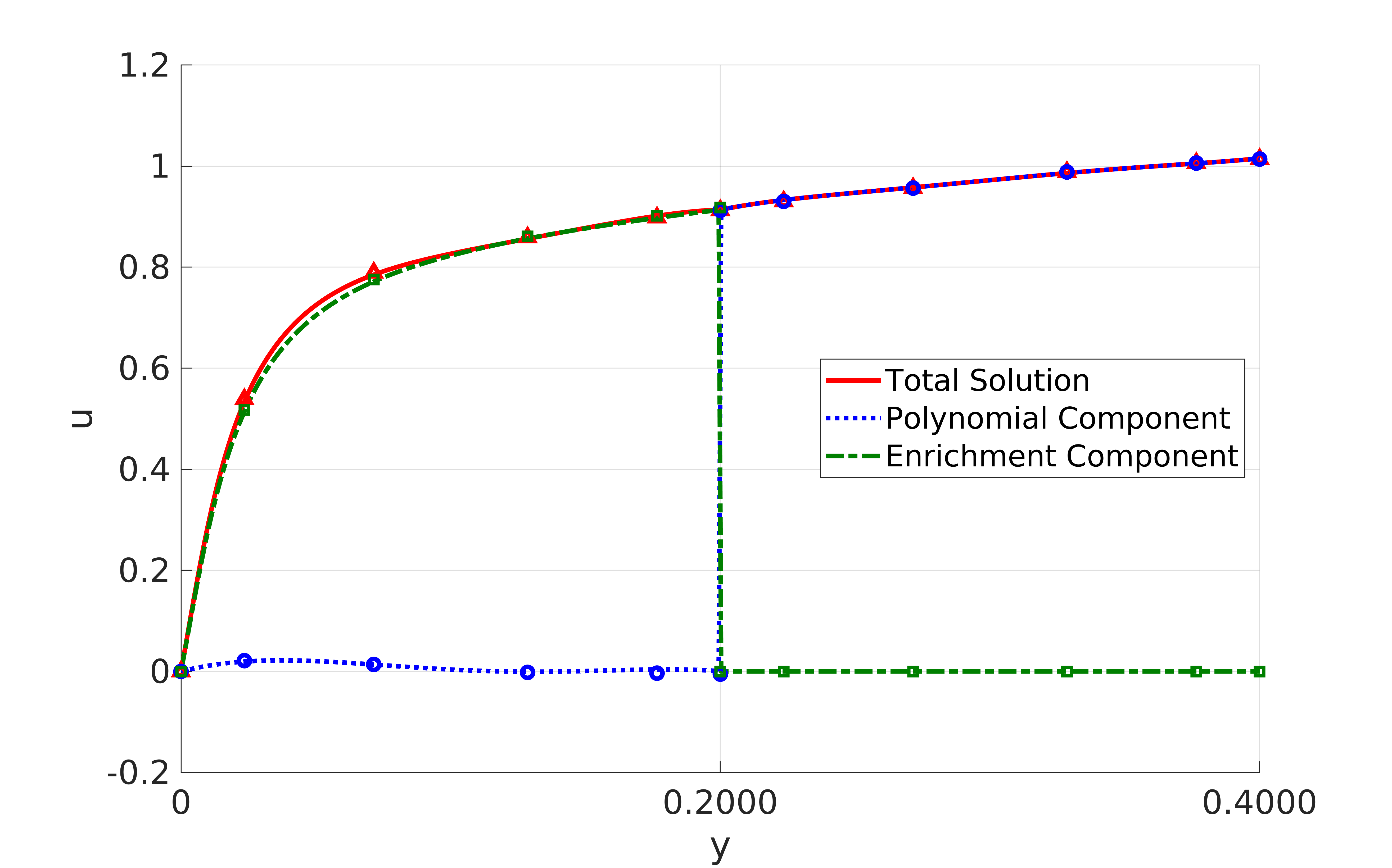
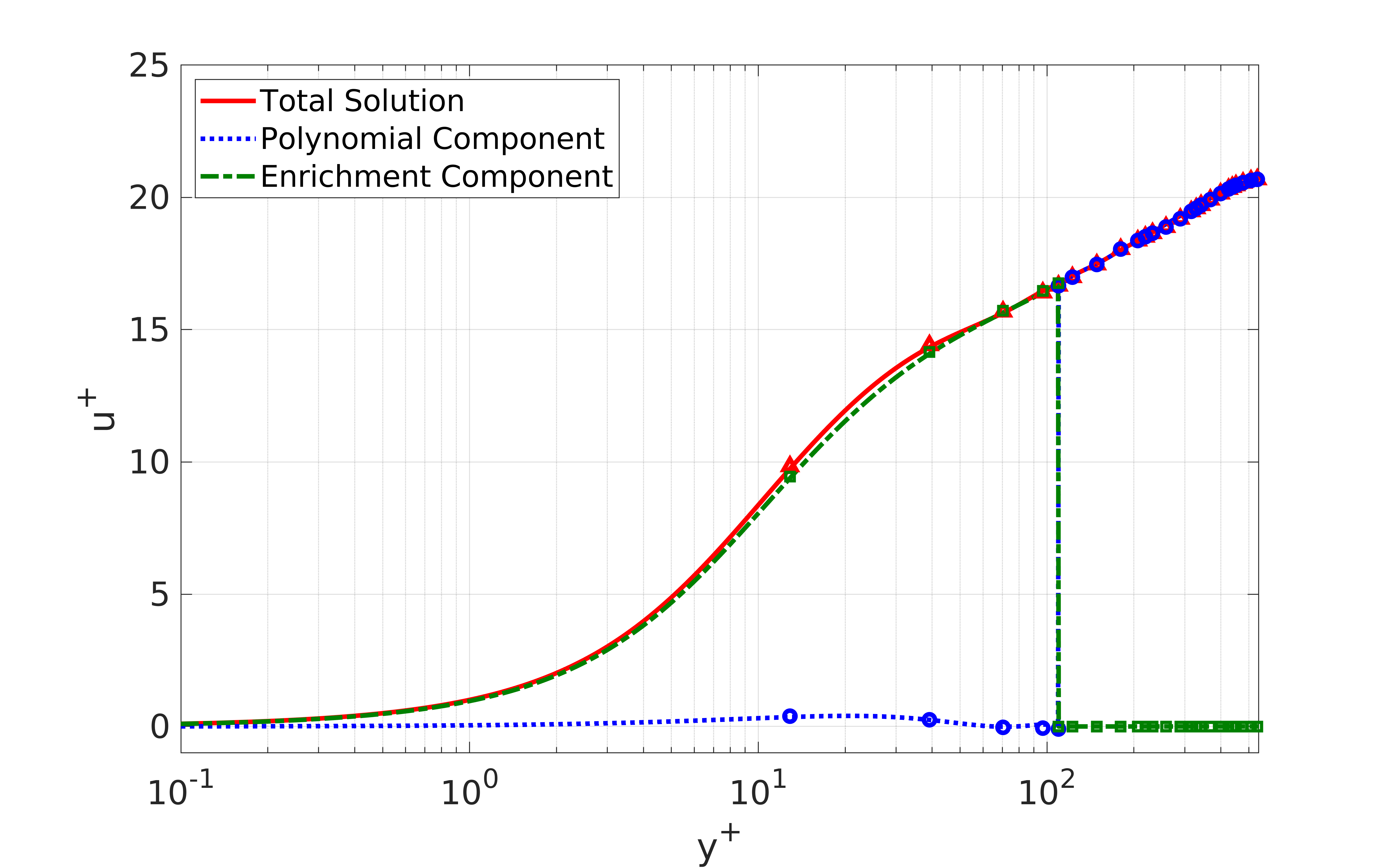
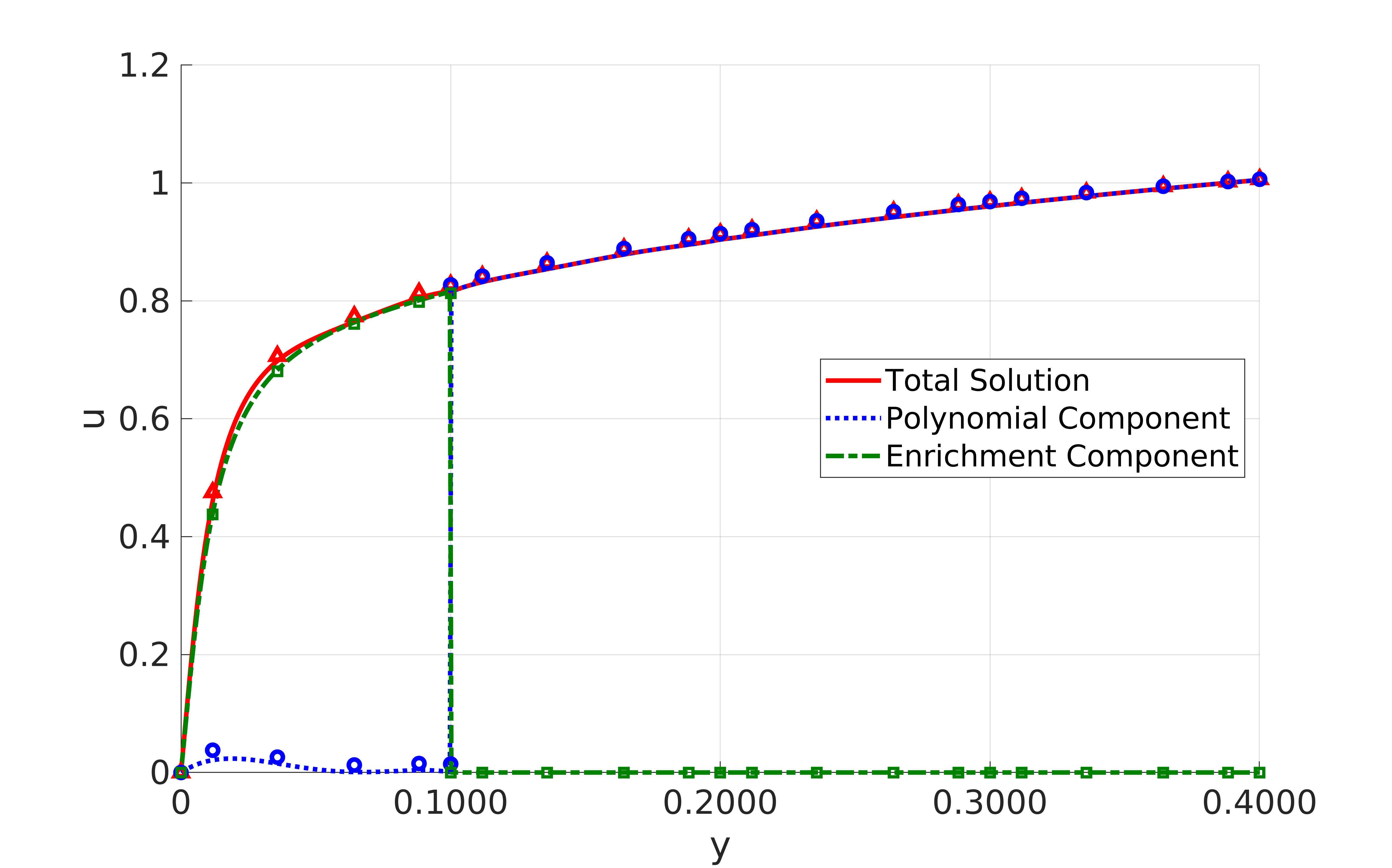
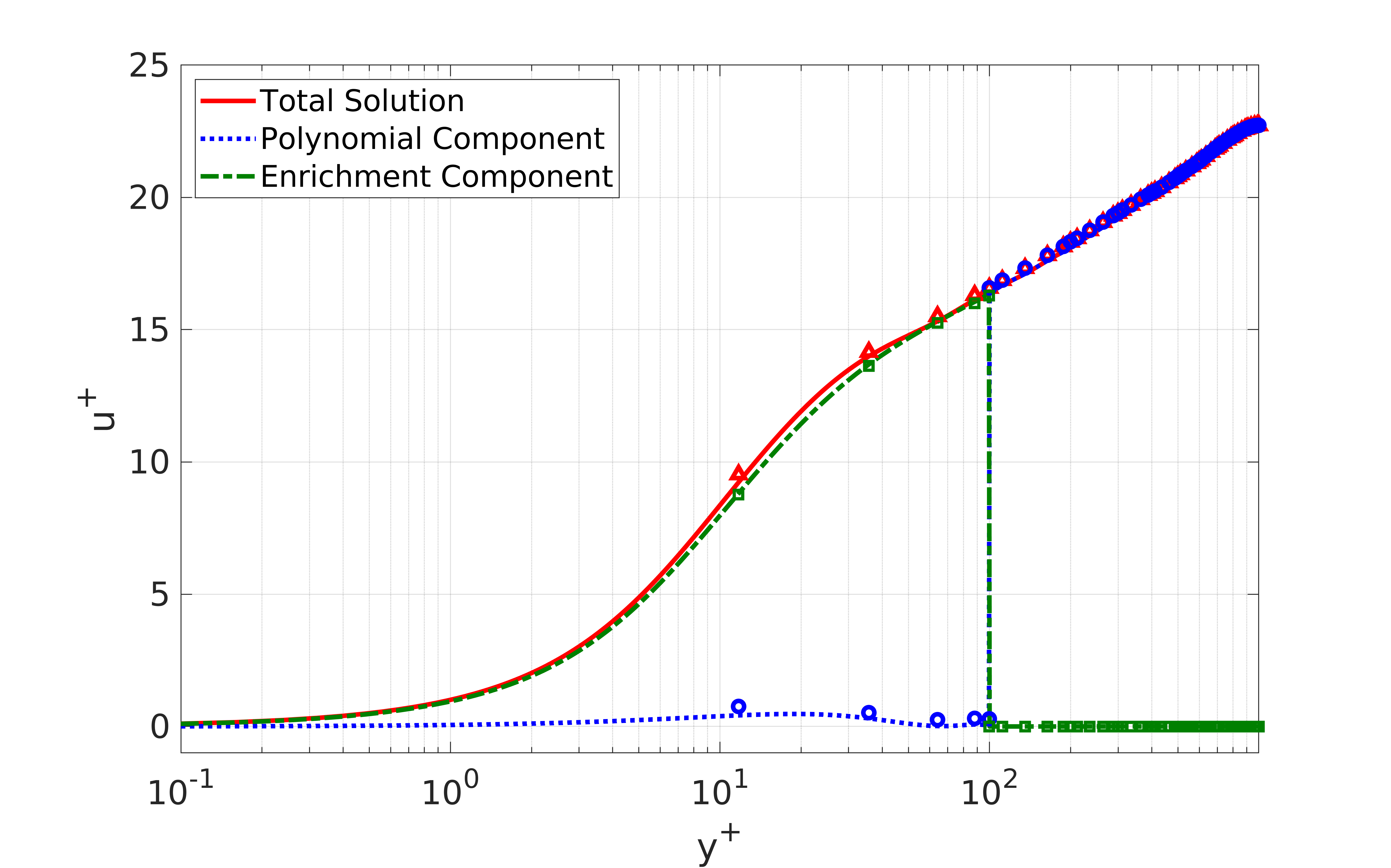
Figure 7: Plots of mean velocity in physical space and plus units broken up into the enrichment and polynomial components. The top plots are for the $Re_{\tau}=543$, $P=5$, $N=10$ case and the bottom plots are for the $Re_{\tau}=1000$, $P=5$, $N=20$ case. In both cases the mean is captured by the enrichment function and the polynomial component has a nearly zero mean from representing the turbulent fluctuations.

6.3 Comparison with Shear Stress Wall-Model

In this section, the enrichment wall-model is compared with purely polynomial standard SEM and a shear stress wall-modeled SEM to show the benefits. All three methods use the same initial conditions and problem specifications from Sec. 6. The standard SEM uses no-slip walls and no added filtering, so the numerics match the enriched case exactly. The shear stress wall-model is implemented as described earlier in [27] [4]. The shear stress wall-model uses no-penetration slip-wall boundary conditions that apply a modeled shear stress at the wall. The matching point is taken as the top of the first wall-adjacent element. The model uses the Reichardt law-of-the-wall as the equilibrium wall-stress model. The initial solution is allowed to develop for $8$ flow-through times before the shear stress wall-model is activated. Additionally, an explicit filter with weight $0.05$ and cutoff ratio $0.65$ are used to add dissipation and greatly decrease the amount of slip at the wall.

Comparisons between the three methods for $Re_{\tau}=2000$, $N=20$, and $P=5,6,7$ are shown in Figures 8-9. The standard SEM struggles to match the DNS mean velocity profile. The $P=5$ case displays oscillations in the first element and over-prediction in the log-layer, while the $P=6$ and $P=7$ cases under-predict the mean velocity. The shear stress wall-model has significant slip at the wall and oscillations in the first element. Then the mean profile is almost entirely missed in the log-layer. On the other hand, the mean velocity profile of the enrichment wall-model is much closer to the DNS data. The rms values show poor performance by the shear stress wall-model as it over-predicts most of the quantities and has oscillatory solutions. For these cases, the enrichment wall-model’s rms data closely resembles the standard SEM. While the enrichment wall-model (ENWM) data improves with refinement in $P$, the method still under-predicts the rms values. In addition, the rms values in the wall-adjacent element are significantly different from the DNS data. For these $Re_{\tau}=2000$ cases, the enrichment wall-model greatly outperforms the other methods. It is able to achieve good agreement with the mean even for low resolutions where the standard SEM and shear stress model struggle. The enrichment model’s no-slip wall is crucial to the accuracy of the mean velocity profile.

Table 2 shows the computed friction velocities for these cases. The enrichment wall-model predicts friction velocities within 2.5% error, while the shear stress wall-model shows errors up to 20% error. As seen in Figs. 8-9, the standard SEM with $N=20$ and $P=6$ shows good agreement with the enrichment method and the DNS. However as $P$ increases, the friction velocity of standard SEM varies largely from the DNS data, showing that this method is not as converged as the enrichment method. The shear stress wall-model only applies the wall stress as a forcing term on the boundary condition and can only use the slip at the wall to prevent oscillations. Hence, for more under-resolved or higher $Re_{\tau}$ cases, the forcing term is not enough to ensure that $u_{\tau}$ is accurately predicted. The strength of the enrichment wall-model for predicting the friction velocity comes from the fact that the modeled wall stress is contained in the physical solution and the enrichment enables it to capture that profile without oscillations.

Comparing the enriched wall-model to the shear stress model and standard SEM demonstrates its strengths as well as some areas where it can be improved. The enrichment method shows significant improvement over the standard SEM in capturing the large gradients in the turbulent boundary layer and improves both the mean velocity profile as well as the rms quantities. Compared to the shear stress wall-model, the enrichment method shows better accuracy in capturing of the mean velocity profile in all regions. Even for the more resolved cases, the shear stress model only captures the log-layer profile and not the near wall region because of the slip at the wall. In the most under-resolved cases, the enrichment wall-model yields better agreement with the rms data than the shear stress model. However, in relatively more resolved cases, the enrichment method under-predicts the rms quantities. Hence, the enrichment wall-model shows improved prediction of the mean velocity, especially in very under-resolved situations, but there is scope for further improvement in capturing the rms quantities of interest which will be pursued in future work. In addition, the extension of the ENWM framework to non-equilibrium boundary layer flows will also be addressed in the future.

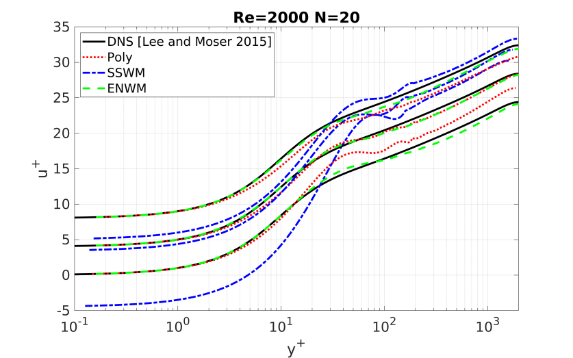
Figure 8: Mean velocity from $Re_{\tau}=2000$ with $N=20$ uniform elements in the channel height and $P=5,6,7$ order basis polynomials with standard SEM (Poly), shear stress wall-model (SSWM), and enrichment wall-model (ENWM). Results with different polynomial orders are shifted up for visibility with $P=5$ on the bottom and $P$ increasing as the results are shifted up by 4. The results are compared with the DNS data from [24].

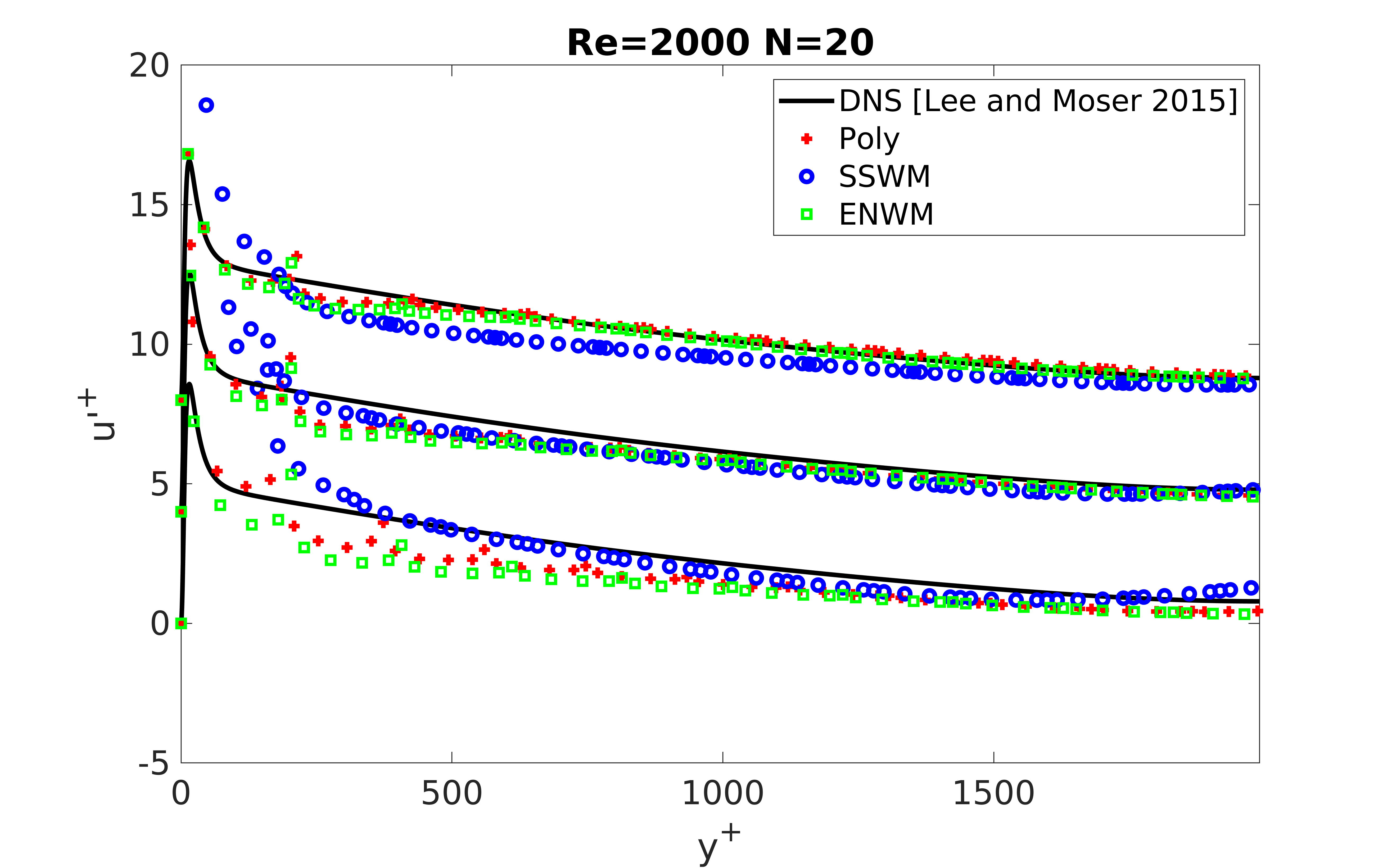
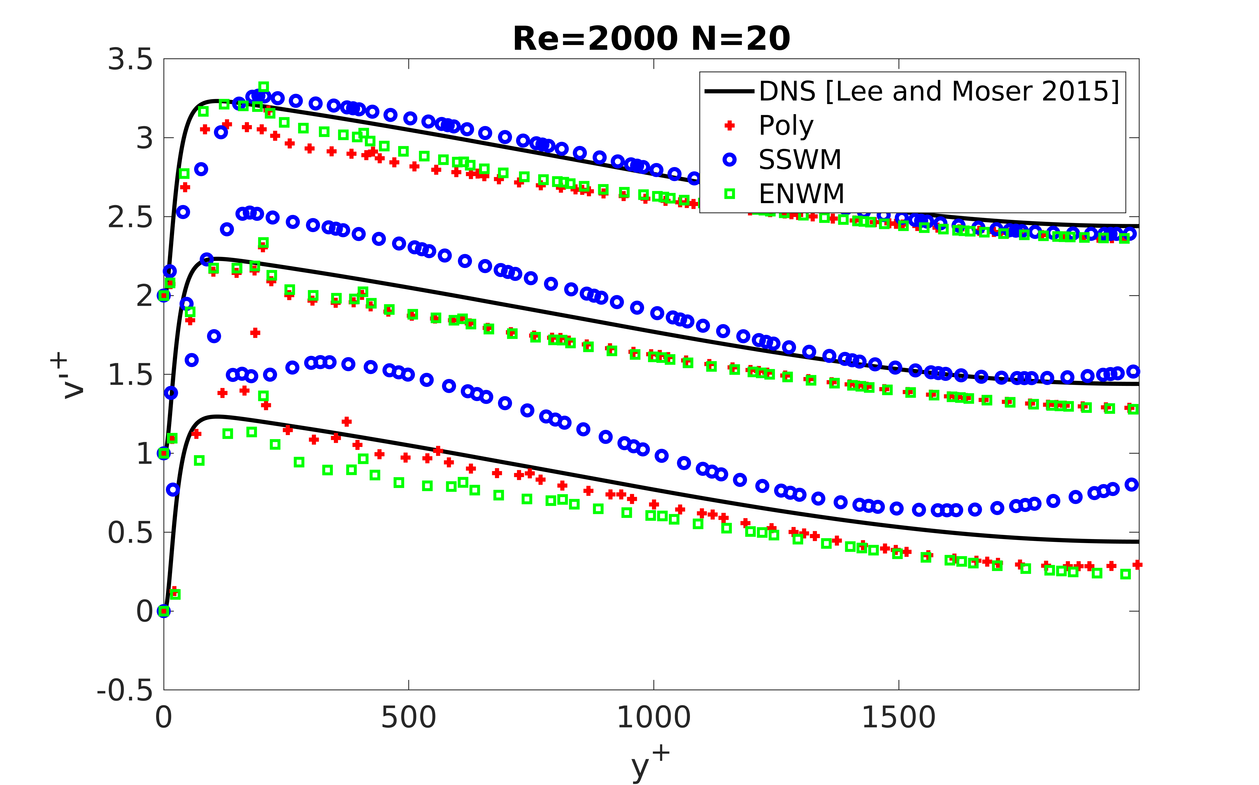
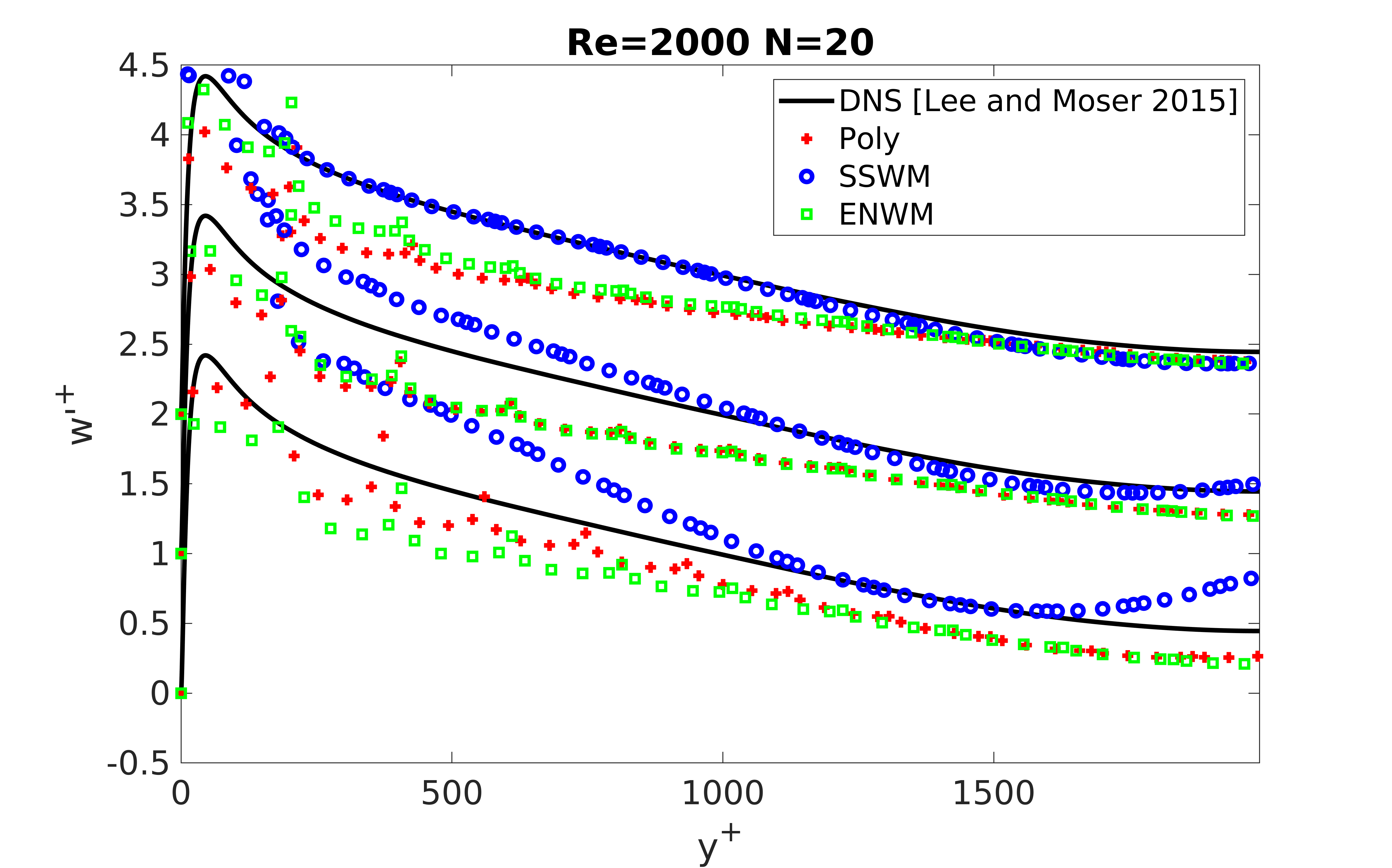
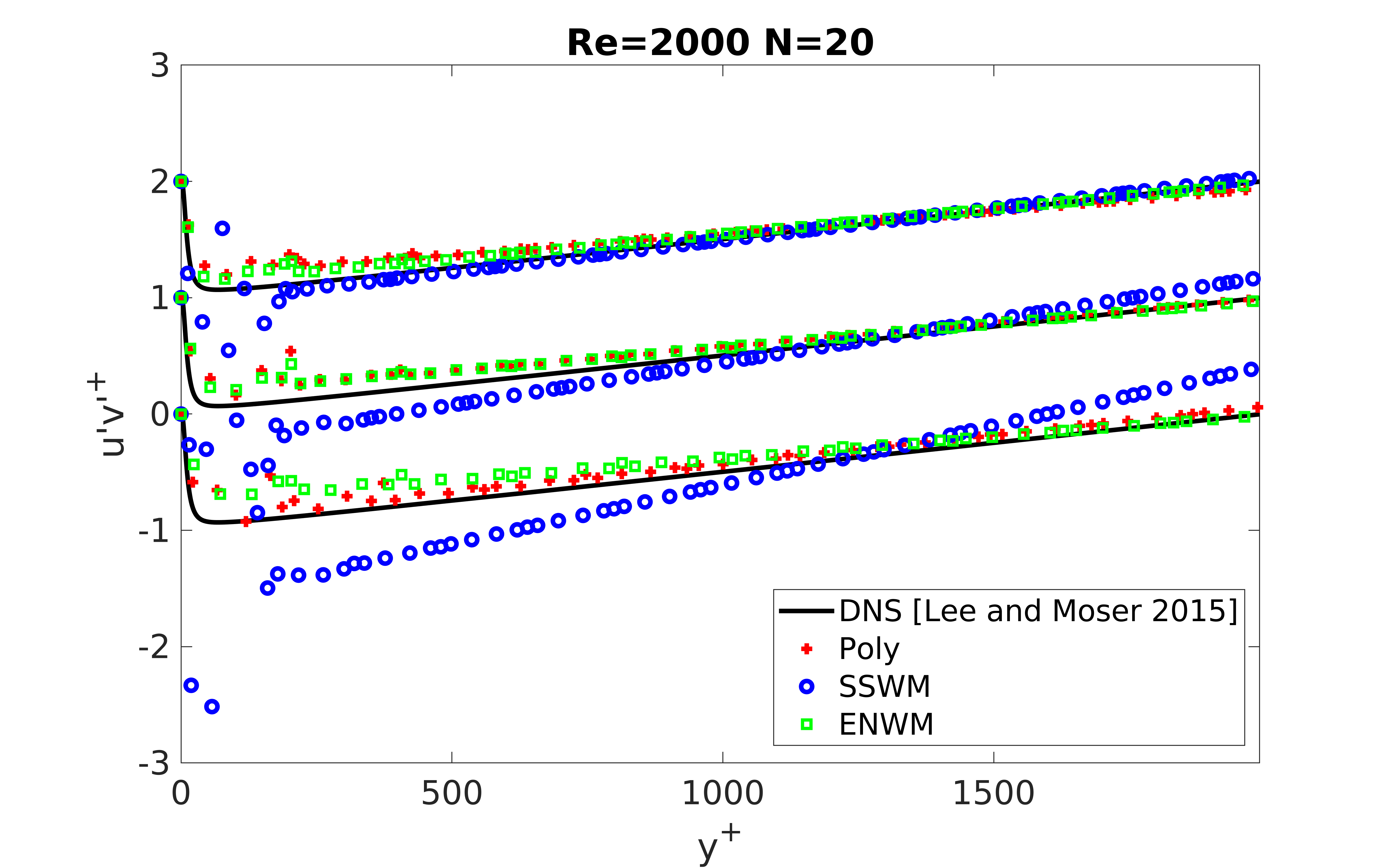
Figure 9: Rms quantities from $Re_{\tau}=2000$ with $N=20$ uniform elements in the channel height and $P=5,6,7$ order basis polynomials with standard SEM (Poly), shear stress wall-model (SSWM), and enrichment wall-model (ENWM). Results with different polynomial orders are shifted up for visibility with $P=5$ on the bottom and $P$ increasing as the results are shifted up by 4 for $u^{\prime+}$ and 1 for the other quantities. The results are compared with the DNS data from [24].

$Re_{\tau}$	$N$	$P$	DNS $u_{\tau}$	Poly $u_{\tau}$	SSWM $u_{\tau}$	ENWM $u_{\tau}$
2000	20	5	0.0459	0.0429	0.0368	0.0468
2000	20	6	0.0459	0.0466	0.0404	0.0467
2000	20	7	0.0459	0.0491	0.0444	0.0469

Table 2: Friction velocity, $u_{\tau}$ for standard SEM (Poly), shear stress wall-model(SSWM), and enrichment wall-model (ENWM) for $Re_{\tau}=2000$. The results are compared with the DNS data from [24].

7 Conclusions

In this work, we proposed an enriched basis wall-modeled LES approach for the spectral element method. The enrichment framework augments the spectral element polynomial basis with a non-polynomial enrichment function. This enrichment function is an analytic law-of-the-wall function for the mean velocity profile in a turbulent boundary layer. Adding this function into the solution representation allows the enrichment to capture the large gradients while the polynomials capture the turbulent fluctuations. Additionally, the augmented solution accurately models the wall shear stresses without modification to the no-slip wall boundary conditions. As a result, the method can simulate high Reynolds number flows with large elements near the wall without unphysical oscillations.

The enrichment wall-model was validated on a range of turbulent channel flow cases. It was shown that the method can accurately capture the mean velocity profile with WMLES of channel flows up to the wall, without an unphysical region that occurs in shear stress wall-models. Compared to SEM with a shear stress wall-model, the enriched model shows a significant improvement in the mean velocity profile for under-resolved cases. There is some underprediction of the rms quantities in the enrichment method, which will be the focus of future work. However, the method shows convergence to the DNS data with increased resolution. The model also demonstrates a separability between the mean flow captured by the enrichment function and the fluctuations captured by the polynomial basis.

8 Acknowledgments

This work was performed under the auspices of the U.S. Department of Energy by Lawrence Livermore National Laboratory under contract DEAC52-07NA27344. This article has been assigned an LLNL document release number LLNL-JRNL-860809-DRAFT. The submitted manuscript has been created by UChicago Argonne, LLC, Operator of Argonne National Laboratory (Argonne). Argonne, a U.S. Department of Energy Office of Science laboratory, is operated under Contract No. DEAC02-06CH11357. The U.S. Government retains for itself, and others acting on its behalf, a paid-up nonexclusive, irrevocable worldwide license in said article to reproduce, prepare derivative works, distribute copies to the public, and perform publicly and display publicly, by or on behalf of the Government. The research work was funded by the DOE project DE-EE0008875. Lastly, the authors would like to acknowledge the computing core hours available through the Bebop cluster provided by the Laboratory Computing Resource Center (LCRC) at Argonne National Laboratory for this research.

References

- Tucker [2013] PG Tucker. Trends in turbomachinery turbulence treatments. Progress in Aerospace Sciences, 63:1–32, 2013.
- Choi and Moin [2012] Haecheon Choi and Parviz Moin. Grid-point requirements for large eddy simulation: Chapman’s estimates revisited. Physics of Fluids, 24(1):011702, 2012.
- Larsson et al. [2016] Johan Larsson, Soshi Kawai, Julien Bodart, and Ivan Bermejo-Moreno. Large eddy simulation with modeled wall-stress: recent progress and future directions. Mechanical Engineering Reviews, 3(1):15–00418, 2016.
- Pal et al. [2021] Pinaki Pal, Muhsin M Ameen, and Chao Xu. Development of wall modeling framework in a high-order spectral element CFD solver Nek5000. In AIAA Scitech 2021 Forum, 2021.
- Lodato et al. [2014] Guido Lodato, Patrice Castonguay, and Antony Jameson. Structural wall-modeled LES using a high-order spectral difference scheme for unstructured meshes. Flow, turbulence and combustion, 92(1-2):579–606, 2014.
- Frère et al. [2017] Ariane Frère, Corentin Carton de Wiart, Koen Hillewaert, Philippe Chatelain, and Grégoire Winckelmans. Application of wall-models to discontinuous Galerkin LES. Physics of Fluids, 29(8):085111, 2017.
- Carton de Wiart and Murman [2017] Corentin Carton de Wiart and Scott M Murman. Assessment of wall-modeled LES strategies within a discontinuous-galerkin spectral-element framework. In 55th AIAA Aerospace Sciences Meeting. AIAA 2017-1223, 2017.
- Lv et al. [2021] Yu Lv, Xiang IA Yang, George I Park, and Matthias Ihme. A discontinuous Galerkin method for wall-modeled large-eddy simulations. Computers & Fluids, 222:104933, 2021.
- Brill and Ihme [2020] Steven Brill and Matthias Ihme. An enriched basis discontinuous Galerkin method for shocks and high-gradient features in fluid mechanics. In AIAA Scitech 2020 Forum. AIAA 2020-1752, 2020.
- Krank and Wall [2016] Benjamin Krank and Wolfgang A Wall. A new approach to wall modeling in LES of incompressible flow via function enrichment. Journal of Computational Physics, 316:94–116, 2016.
- Krank et al. [2018] Benjamin Krank, Martin Kronbichler, and Wolfgang A Wall. Wall modeling via function enrichment within a high-order DG method for RANS simulations of incompressible flow. International Journal for Numerical Methods in Fluids, 86(1):107–129, 2018.
- Krank et al. [2019] Benjamin Krank, Martin Kronbichler, and Wolfgang A Wall. A multiscale approach to hybrid RANS/LES wall modeling within a high-order discontinuous galerkin scheme using function enrichment. International Journal for Numerical Methods in Fluids, 90(2):81–113, 2019.
- Lottes and Kerkemeier [2008] Paul F. Fischer James W. Lottes and Stefan G. Kerkemeier. nek5000 Web page, 2008. http://nek5000.mcs.anl.gov.
- Deville et al. [2002] Michel O Deville, Paul F Fischer, Paul F Fischer, EH Mund, et al. High-order methods for incompressible fluid flow. Cambridge University Press, 2002.
- Ascher and Greif [2011] Uri M Ascher and Chen Greif. A first course on numerical methods. SIAM, 2011.
- Maday and Rønquist [1990] Yvon Maday and Einar M Rønquist. Optimal error analysis of spectral methods with emphasis on non-constant coefficients and deformed geometries. Computer Methods in Applied Mechanics and Engineering, 80(1-3):91–115, 1990.
- Karniadakis and Sherwin [2005] George Karniadakis and Spencer Sherwin. Spectral/hp Element Methods for Computational Fluid Dynamics. Oxford University Press, 06 2005.
- Kirby and Karniadakis [2003] Robert M Kirby and George Em Karniadakis. De-aliasing on non-uniform grids: algorithms and applications. Journal of Computational Physics, 191(1):249–264, 2003.
- Fischer et al. [2017] Paul Fischer, Martin Schmitt, and Ananias Tomboulides. Recent developments in spectral element simulations of moving-domain problems. In Recent Progress and Modern Challenges in Applied Mathematics, Modeling and Computational Science, pages 213–244. Springer, 2017.
- Patera [1984] Anthony T Patera. A spectral element method for fluid dynamics: laminar flow in a channel expansion. Journal of Computational Physics, 54(3):468–488, 1984.
- Ching et al. [2020] Eric J. Ching, Steven R. Brill, Michael Barnhardt, and Matthias Ihme. A two-way coupled Euler-Lagrange method for simulating multiphase flows with discontinuous Galerkin schemes on arbitrary curved elements. Journal of Computational Physics, 405:109096, 2020. ISSN 0021-9991.
- Brill et al. [2022] Steven Brill, Pinaki Pal, Muhsin Ameen, Chao Xu, and Matthias Ihme. An enrichment wall model for the spectral element method. In AIAA Scitech 2022 Forum, 2022.
- Scalo et al. [2015] Carlo Scalo, Julien Bodart, and Sanjiva K Lele. Compressible turbulent channel flow with impedance boundary conditions. Physics of Fluids, 27(3):035107, 2015.
- Lee and Moser [2015] Myoungkyu Lee and Robert D. Moser. Direct numerical simulation of turbulent channel flow up to . Journal of Fluid Mechanics, 774:395–415, 2015. doi: 10.1017/jfm.2015.268.
- Fang et al. [2011] Jiannong Fang, Marc Diebold, Chad Higgins, and Marc B Parlange. Towards oscillation-free implementation of the immersed boundary method with spectral-like methods. Journal of Computational Physics, 230(22):8179–8191, 2011.
- Gillyns et al. [2022] Emmanuel Gillyns, Sophia Buckingham, and Grégoire Winckelmans. Implementation and validation of an algebraic wall model for LES in Nek5000. Flow, Turbulence and Combustion, pages 1–21, 2022.
- Pal et al. [2022] Pinaki Pal, Muhsin Ameen, and Chao Xu. Near-wall modeling of turbulent flow and heat transfer using a spectral element CFD solver. In AIAA Scitech 2022 Forum, 2022.