Prepared for the Worst: A Learning-Based Adversarial Attack for Resilience Analysis of the ICP Algorithm

Abstract

This paper presents a novel method to assess the resilience of the Iterative Closest Point (ICP) algorithm via deep-learning-based attacks on lidar point clouds. For safety-critical applications such as autonomous navigation, ensuring the resilience of algorithms prior to deployments is of utmost importance. The ICP algorithm has become the standard for lidar-based localization. However, the pose estimate it produces can be greatly affected by corruption in the measurements. Corruption can arise from a variety of scenarios such as occlusions, adverse weather, or mechanical issues in the sensor. Unfortunately, the complex and iterative nature of ICP makes assessing its resilience to corruption challenging. While there have been efforts to create challenging datasets and develop simulations to evaluate the resilience of ICP empirically, our method focuses on finding the maximum possible ICP pose error using perturbation-based adversarial attacks. The proposed attack induces significant pose errors on ICP and outperforms baselines more than 88% of the time across a wide range of scenarios. As an example application, we demonstrate that our attack can be used to identify areas on a map where ICP is particularly vulnerable to corruption in the measurements.

I Introduction

The Iterative Closest Point (ICP) algorithm has become a fundamental localization algorithm in mobile robotics [1] [2]. ICP computes a robot’s current pose by determining the transformation that optimally aligns the scan point cloud (robot’s current view) with a map point cloud. At the same time, lidar sensors have emerged as the predominant choice for robot localization and mapping [3]. However, despite its popularity, lidar-based ICP is prone to failures in challenging scenarios, such as those with adverse weather or significant occlusions [4] [5]. Figure 1 illustrates how landmarks needed for localization can be occluded in typical autonomous driving conditions. With fewer landmarks to rely on, ICP can become more susceptible to other corruption in the measurements, leading to high estimate errors. Moreover, when an obstacle occludes landmarks in its proximity, ICP may wrongly identify it as part of the map. In such cases, ICP attempts to align the obstacle’s points in the scan to the map, leading to an error in the pose estimate. Similar errors can arise in adverse weather conditions. For instance, when the wind carries snow into the proximity of landmarks, it becomes difficult for ICP to distinguish and filter the snow from the landmarks.

This calls for reliable ICP evaluation methods to ensure the safe deployment of autonomous robots into the real world. These methods need to accurately inform us about the types of errors that can be expected during deployment, considering the possibility of adverse weather or occlusions.

To this end, adverse weather datasets such as Boreas [6] and CADC [7] have been collected, and prior works [4] [8] have evaluated lidar-based localization on these datasets. Additionally, [5] simulated occlusion cases in cities and used them to evaluate the performance of lidar-based localization algorithms under occlusion. Although datasets and simulations can give us valuable insights into ICP’s resilience, neither can inform us of lidar-based ICP’s worst-case performance, which is particularly crucial in safety-critical applications such as autonomous navigation.

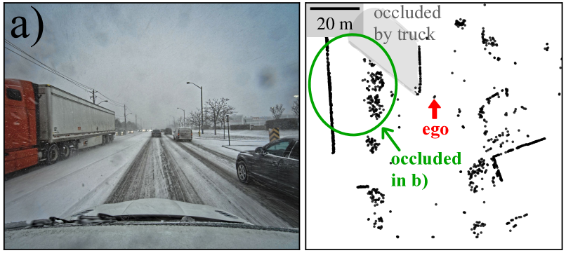
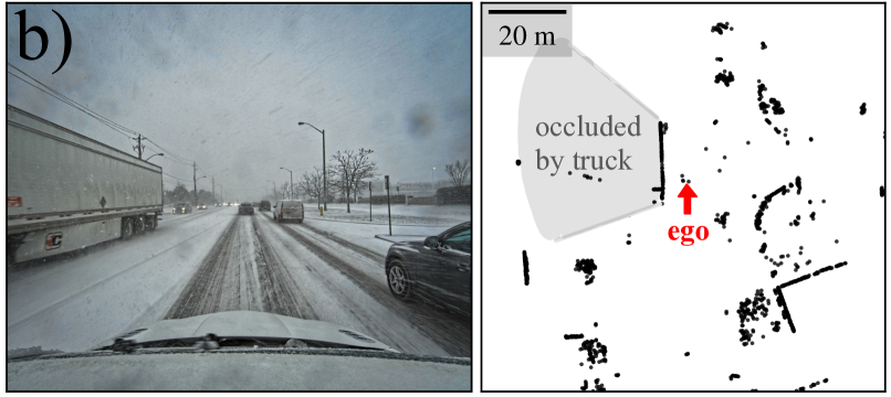
Figure 1: Illustrative occlusion scenarios from the Boreas dataset [6] where the ego vehicle encounters occlusion caused by a truck. Camera images for two scenarios are shown on the left, with corresponding lidar scans captured at the same time on the right. Scenario a) precedes b) by 0.3 seconds. The ground planes in the lidar scans are removed for clarity. The pose of the ego vehicle and the region occluded by the truck are annotated with a red arrow and a gray sector, respectively. When the truck occludes the green-circled landmarks in b), the ICP algorithm may mistake the truck for the circled landmarks in its calculations, resulting in a significant error in the pose estimate.

While [9] previously presented an analytic approach to bridge this gap, we propose a learning-based approach with the advantage of requiring fewer assumptions and approximations. In this paper, we propose to investigate the worst-case performance of ICP via a generative network that deliberately perturbs measured scans to maximize the pose error of ICP, while keeping the perturbations within a specified bound. Once trained, our network can estimate the maximum pose error arising from perturbations in a new scan. We evaluate our approach by attacking point-to-plane ICP on the ShapeNetCore [10] and Boreas [6] datasets. Our approach consistently outperforms baselines and learns non-trivial perturbations.

Our contributions are two-fold:

• To the best of our knowledge, we propose the first learning-based adversarial attack against lidar-based ICP.

• We present a novel way to quantitatively assess the resilience and worst-case performance of the ICP algorithm. We show, through extensive experiments on the Boreas dataset, the worst-case ICP pose errors that our model can induce in urban autonomous driving environments. As part of this, we identify locations susceptible to unusually high pose errors in the presence of measurement corruption.

II Related Work

II-A Analysis on ICP in Challenging Environments

When robots are deployed in the real world, they must operate robustly in challenging situations. Environments particularly challenging to ICP include those with geometric degeneracy, occlusions, and adverse weather conditions.

Geometrically under-constrained environments refer to environments with very limited or degenerate geometric constraints for registration such as tunnels and narrow corridors. Under-constrained environments have long been established as a major source of ICP error [11]. Numerous studies, such as [12] [13] [14] [15], have investigated ICP’s performance in such environments and proposed solutions. In comparison, ICP’s robustness under occlusions and adverse weather is less studied and is the focus of this paper.

It was suspected that lidar-based localization would suffer in adverse weather conditions (e.g., rain, snow, and fog) as works such as [16] showed that lidar sensor performance degrades in adverse weather. Putting lidar-based localization to the test, [8] conducted an extensive evaluation of a lidar-based localization system on the all-weather Boreas dataset [6]. They found that lidar-based localization is surprisingly robust to moderate precipitation. Later, [4] evaluated lidar-based ICP over the Canadian Adverse Driving Conditions (CADC) dataset [7] and also discovered that lidar-based ICP is robust to a high level of precipitation. However, they observed that extreme, abrupt cases such as snow gusts led to significant ICP localization errors. Due to an insufficient amount of data on these extreme cases, they could not quantitatively evaluate the impact of these extreme events on ICP.

[4] identified view obstruction (occlusion) as another event that led to large pose errors. [5] presented a comprehensive evaluation of lidar-based localization under occlusions through simulation. Unsurprisingly, they found that, on average, localization error increases with the percentage of the scene being occluded and significant localization errors can arise when half or more of the scene is occluded.

Knowing that occlusions and adverse weather can cause substantial localization errors, being able to predict the maximum possible ICP pose error becomes a matter of great interest. [9] previously proposed an analytic, closed-form method for estimating the maximum expected ICP error that can arise from corrupted measurements. This paper differs from [9] in two main ways. First, [9] corrupted only a sector of the scan, whereas we can corrupt the entire point cloud. This enables us to model more diverse scenarios (e.g., occlusions in multiple sectors or precipitation that tends to corrupt all sectors) and makes our approach more suitable for worst-case analysis. Secondly, our data association is re-calculated at every ICP iteration, whereas in [9] a known data association is assumed.

II-B Adversarial Attacks Against Autonomous Driving Systems

Adversarial attacks that deliberately craft examples to undermine the target algorithm’s performance are very suitable for our purpose of worst-case analysis. Many point cloud adversarial attacks have been proposed against different components of the autonomy stack. [17] introduced novel frameworks for attacking algorithms processing 3D point clouds. These attacks work via point addition, point removal, and gradient-based point perturbation. [18] proposed the first generative attack against point cloud classification algorithms via point perturbation. They showed that generative approaches are much faster than gradient-based approaches while upholding good attack performance. For this reason, and the resemblance of our task to theirs, our architecture draws inspiration from theirs.

In the object detection domain, [19] discovered that detection models tend to ignore occlusion patterns in the point clouds and introduced a black-box attack exploiting this vulnerability. [20] proposed an attack that perturbs vehicle trajectories to maximize the errors of trajectory prediction algorithms. They also leveraged the attack to assess how worst-case predictions would affect downstream tasks. They successfully increased the prediction errors by more than 150% and showed that worst-case predictions have critical safety concerns. Their work supports our proposal of using adversarial attacks for worst-case performance analysis. While we draw inspiration from these works, they are not attacking localization algorithms.

For attacks against localization algorithms, [21] presented how to use infrared light to mislead camera-based SLAM. On lidar-based SLAM specifically, [22] demonstrated the feasibility of introducing false loop-closure detection by increasing the similarity between two distinct locations using physical objects. Our work differs from these works in that we are not merely introducing errors in the target algorithm but rather maximizing its error. Moreover, their target algorithms and attack mechanisms significantly differ from ours.

Most similar to our work, [23] proposed a method for misleading lidar-based ICP to a specific wrong pose via adversarial point perturbation. However, their method is iterative and gradient-based, while ours is learning-based. As shown in [18], learning-based approaches are much faster. [23] is also limited to 2D lidar scans and tampers only with the distance, not the angle, of points. Our work operates on both 2D and 3D lidar scans and can perturb both the distance and the angle. To the best of our knowledge, we propose the first learning-based adversarial attack against lidar-based ICP.

III Theory

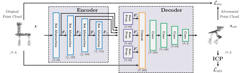
Figure 2: Overview of the proposed attack pipeline. Given an input point cloud $\bm{X}$, the encoder extracts hierarchical features from it using set-abstraction modules from the PointNet++ [24] architecture. The decoder interpolates the extracted features and uses them along with the original point cloud to produce an adversarial point cloud $\bm{X}_{\text{adv}}$ to attack ICP. The encoder and decoder together form the generator $\bm{G}$, which is trained using reconstruction loss and adversarial loss.

This section is an overview of our proposed attack. Our overall pipeline is visualized in Figure 2. We propose a generative network that learns how to perturb a point cloud to maximize the pose error of ICP while keeping the perturbations within a specified bound.

III-A Attack Target: ICP

Our model can attack any lidar-based ICP algorithm. However, we need differentiable versions of ICP to train. We train using dICP [25], which supports differentiable ICP and the use of trim distance and robust cost functions. Note that we attack the single-frame ICP algorithm on its own, rather than a full localization pipeline (e.g., with odometry), which we leave for future work.

Given a reference point cloud (also known as the map) $\bm{Q}\in\mathbb{R}^{M\times 3}$ and a measured point cloud (also known as the scan) $\bm{P}\in\mathbb{R}^{N\times 3}$, ICP estimates a transform from the scan to the map ${\bm{{\hat{T}}_{QP}}}\in SE(3)$. $M,N\in\mathbb{N}$ denote the number of points in the map and scan, respectively. The ICP pose error vector $\bm{\xi}\in\mathbb{R}^{6}$ can be calculated using the ground truth transform $\bm{T_{QP}}\in SE(3)$ via

$$\bm{\xi}=\begin{bmatrix}\bm{\rho}\\ \bm{\phi}\end{bmatrix}=\log\left(\bm{{\hat{T}}_{QP}}\bm{{T_{QP}}}^{-1}\right)^{\vee},$$ (1)

where $\bm{\rho}\in\mathbb{R}^{3}$ is the translation component of the error and $\bm{\phi}\in\mathbb{R}^{3}$ is the rotation component of the error. Here, $\log(\cdot)$ maps an $SE(3)$ element to its lie algebra $\mathfrak{se}(3)$ and $(\cdot)^{\vee}$ maps an $\mathfrak{se}(3)$ element to $\mathbb{R}^{6}$ [26].

III-B Attack model

Our model is a generator $\bm{G}$ consisting of an encoder and a decoder. The encoder is based on PointNet++ [24] and learns to extract hierarchical features from an input point cloud $\bm{X}\in\mathbb{R}^{N\times 3}$. Using the extracted features, the decoder learns how to perturb $\bm{X}$ to get $\bm{X}_{\text{adv}}\in\mathbb{R}^{N\times 3}$. This architecture is inspired by LG-GAN [18], which successfully attacked 3D point cloud classification algorithms via perturbation.

III-B1 Encoder

Hierarchical features provide rich representations of the point cloud, encompassing global and local aspects. To extract hierarchical features, we design the encoder with four cascaded PointNet++ [24] set-abstraction modules, as shown in Figure 2. A set-abstraction module takes a set of points and samples a smaller set using farthest-point sampling. Every sampled point embeds local patterns around it by learning to effectively aggregate features of its neighboring points in the original set. Subsequently, this subset of points along with newly learned features are fed into the next set-abstraction module. By stacking set-abstraction modules one on top of another, a hierarchy of features of various scales can be extracted. Precisely, the encoder extracts features of four scales: $\bm{F}_{1}\in\mathbb{R}^{N\times 64}$, $\bm{F}_{2}\in\mathbb{R}^{\frac{N}{a}\times 128}$, $\bm{F}_{3}\in\mathbb{R}^{\frac{N}{b}\times 256}$, and $\bm{F}_{4}\in\mathbb{R}^{\frac{N}{c}\times 512}$ where $a,b,c\in\mathbb{R}$ are manually selected hyperparameters.

III-B2 Decoder

When decoding, we want to leverage information at all scales. However, higher-level features are sparser and not available for every point in the original point cloud $\bm{X}$. Therefore, $\bm{F}_{2}$, $\bm{F}_{3}$, and $\bm{F}_{4}$ are interpolated. The procedure for interpolation is as follows. For every point in $\bm{X}$, higher-level features of $k$-nearest neighbors are weighted inverse-proportionally to their distances and summed. These weighted sums are then concatenated with features in $\bm{F}_{1}$. The concatenated features are passed through neural network layers, which turn the features into more compact sizes of $N\times 64$. Finally, interpolated $\bm{F}_{2}^{\prime},\bm{F}_{3}^{\prime},\bm{F}_{4}^{\prime}\in\mathbb{R}^{N\times 64}$ and $\bm{X}$ are concatenated together and passed through four 1D convolution layers to generate the adversarial point cloud ${\bm{X}}_{\text{adv}}$.

III-C Loss function

The loss function is a weighted sum of two component losses: adversarial loss $\mathcal{L}_{\text{adv}}$ and reconstruction loss $\mathcal{L}_{\text{rec}}$. That is

$$\mathcal{L}=\alpha\mathcal{L}_{\text{adv}}+\beta\mathcal{L}_{\text{rec}},$$ (2)

where $\alpha,\beta\in\mathbb{R}$ are manually selected hyperparameters. The adversarial loss guides the generator G to generate $\bm{X}_{adv}$, which when used as a scan in ICP will maximize ICP pose error. Therefore, $\mathcal{L}_{\text{adv}}$ is defined as

$$\begin{split}\mathcal{L}_{\text{adv}}=&-{\left\lVert\begin{bmatrix}w_{1}\\ w_{2}\\ w_{3}\\ \end{bmatrix}^{\top}\bm{\rho}\right\rVert_{2}}-\left\lVert\begin{bmatrix}w_{4}\\ w_{5}\\ w_{6}\\ \end{bmatrix}^{\top}\bm{\phi}\right\rVert_{2},\end{split}$$ (3)

where $w_{i}\in\mathbb{R}$ for $i=\text{1, ..., 6}$ specify the weight of each pose error element. The ICP error is split into the translation component $\bm{\rho}\in\mathbb{R}^{3}$ and the rotation component $\bm{\phi}\in\mathbb{R}^{3}$.

On the other hand, $\mathcal{L}_{\text{rec}}$ is in place to bind the perturbations G is allowed to introduce. Perturbations that are too extreme are unlikely to happen in reality and will make our worst-case analysis too pessimistic to be useful. For ICP algorithms with trimming, the trim distance already prevents points from being moved excessively far away. However, a point can be moved beyond the trim distance from its original association but still fall within the trim distance of other points in the map. It will then become re-associated with one of those points. Therefore, relying solely on the trim distance may lead to perturbations that are unrealistically or undesirably large. To address this issue, $\mathcal{L}_{\text{rec}}$ is proposed as

$$\mathcal{L}_{\text{rec}}=\frac{1}{N}{\sum_{i=1}^{N}S(\|\bm{x}_{i}-(\bm{x_{\text{Adv}}})_{i})\|_{2})^{2}},$$ (4)

where $\bm{x}_{i}$ is a point in $\bm{X}$ and $(\bm{x_{\text{adv}}})_{i}$ is the corresponding point in $\bm{X}_{\text{adv}}$. $S(\cdot)$ is the SoftShrinkage function defined as

$$S(z)=\begin{cases}z-\lambda,&\text{if }z>\lambda\\ z+\lambda,&\text{if }z<-\lambda\\ 0,&\text{otherwise.}\end{cases}$$ (5)

The manually selected parameter $\lambda\geq 0$ represents the perturbation bound.

IV Experiments

This section details the experiment setup and results. We present qualitative and quantitative results on both the ShapeNetCore [10] and Boreas [6] datasets.

IV-A Datasets

We evaluate our attack on two datasets — ShapeNetCore [10] and Boreas [6]. The ShapeNetCore dataset is a subset of the ShapeNet dataset that consists of 3D point clouds of simple objects. Due to its simplicity, we use the ShapeNetCore dataset to examine the inner workings of our model and qualitatively compare our model with the baselines. Despite the 3D nature of the ShapeNetCore dataset, we cast them to 2D for better interpretation. Furthermore, we normalize the point clouds to fit within a unit circle at the origin. We use the full point clouds as maps and randomly sample 2048 points from the maps to create scans. We add normally distributed noise with a zero mean and 0.025 standard deviation to the scans to prevent perfect alignment. Finally, a small, random transformation is applied to each scan. The transformation consists of uniformly distributed translations from -0.08 to 0.08 along the $x$-axis and the $y$-axis as well as a uniformly distributed rotation from -10 to 10 degrees around the $z$-axis. This transformation serves as the ground truth pose. The transformations are kept small such that the ICP algorithm can use no motion for its initial guesses.

To assess our attack’s effectiveness for autonomous navigation applications, we further evaluate our attack on the Boreas dataset [6], an all-weather autonomous driving dataset collected by driving a repeated route over one year. The Boreas dataset is chosen for its abundant data with occlusions and adverse weather. We use the Teach and Repeat [27] framework to establish localization pairs on the Boreas dataset, following the procedure described in [8]. Teach and Repeat first conducts a teach pass along a route to construct a map, to which the subsequent repeat passes along the same route can be localized. The sequence of lidar point clouds gathered during the teach pass is processed into submaps. The sequences of lidar point clouds captured during the repeat passes, the “live scans”, are localized against the spatially closest submaps. Once localization pairs are generated, we preprocess them to use for training our network. First, we align the live scans with the corresponding submaps using the ground truth poses. Then we apply a small, random transformation to each live scan to generate the final scan we task ICP to localize. The transformations involve random translations, uniformly distributed from -0.3 to 0.3 meters, along the $x$-axis, $y$-axis, and $z$-axis, as well as random rotations, uniformly distributed from -10 to 10 degrees, around the $x$-axis, $y$-axis, and $z$-axis.

IV-B Baselines

Given the absence of established baselines in both ICP worst-case analysis and adversarial attacks against ICP, we compare our approach with straightforward yet effective heuristic baselines. A brief comparison to [9] is provided in Section IV-D4.

IV-B1 Uniform Translation Baseline

The first baseline we adopt uniformly translates the entire scan by the maximum allowed perturbation, $\lambda$, at random angles in the $x-y$ plane. The perturbations are restricted to the $x-y$ plane because we focus on the lateral and longitudinal localization errors a model can induce. These errors are more significant than vertical pose errors in autonomous navigation applications.

IV-B2 Normal Translation Baseline

Another baseline we compare to moves points in the scan by $\lambda$ in the direction of their normal vectors projected onto the $x-y$ plane. We hypothesize that this will be more effective than the uniform translation baseline in attacking point-to-plane ICP that aims to minimize the normal distance from each point in the scan to the tangent plane of the corresponding point in the map. Moreover, [9] shows that shifting measured points along the normal vectors of their associated map points is an effective attack on point-to-plane ICP.

As the normal vectors are bidirectional, we need to unify their directions. When the $x$-component of the normal vector is zero, the vector is flipped such that its $y$-component is positive. When the $x$-component is non-zero, the vector is flipped such that its $x$-component is positive.

Figure 3: A qualitative comparison between the original point clouds and the adversarial point clouds produced by our model and the baselines. Columns 2 through 6 showcase the adversarial point clouds resulting from applying our models and the baselines to the original point clouds in column 1. The adversarial point clouds are coloured according to the angle of the displacement vectors, $\bm{X}_{\text{adv}}-\bm{X}$. The heading pose error and the norm of the lateral and longitudinal pose errors of ICP induced by each point cloud are indicated at the upper and lower right corners, respectively. The lateral and longitudinal pose errors are unitless as the original point clouds are normalized to fit within a unit circle centered at the origin. Minor ICP pose errors are observed even when localizing the original, uncorrupted point clouds in column 1. This is due to the intentional addition of noise to the scans, aimed at preventing perfect alignment between the scans and the maps.

IV-C ShapeNetCore Results

IV-C1 Implementation Details

We train our models on approximately 8900 ShapeNetCore samples using a batch size of 32. We determine empirically that the optimal values for hyperparameters $a,b,c$ are $2,4,8$, respectively, conditioned on the rest of our settings. For $\mathcal{L}_{\text{Adv}}$, we set $\alpha=1$ and $\beta=10$. It takes around 22 epochs to converge. We use the AdamW [28] optimizer with a StepLR scheduler that reduces the initial learning rate of $10^{-4}$ by 30% every 7 epochs.

Before training, we pretrain the generator G for 50 epochs on the training dataset with $\alpha=0$ and $\beta=1$, essentially asking it to reconstruct the original scans. Without pretraining, G generates scans that are too different from the maps to extract meaningful gradients from ICP.

The ICP algorithm under attack is of type point-to-plane. We limit its maximum number of iterations to 25 to expedite training. For testing, we set the maximum number of iterations to 150, which we verify to be more than enough for ICP to converge with an error tolerance of $10^{-4}$ in most cases. Samples where ICP does not converge are dropped. The ICP algorithm is also equipped with a Cauchy robust cost function with the Cauchy parameter set to 0.15 and a trim filter with the trim distance set to 0.3. These parameters are chosen according to common practices.

IV-C2 Case Study on Weights in the Adversarial Loss

This section explores how weights in the adversarial loss (3) affect the kind of perturbations our model learns. We train our model on the ShapeNetCore dataset in three settings. In the $\theta-only$ setting, we set $w_{6}=1$ and all other weights $w_{1}=w_{2}=w_{3}=w_{4}=w_{5}=0$. The $x-only$ setting uses only the $x$-axis translation error in $\mathcal{L}_{\text{Adv}}$ by setting $w_{1}=1$ and all other weights to 0. Finally, the $x-y$ setting uses both $x$-axis and $y$-axis translation errors in $\mathcal{L}_{\text{Adv}}$ (i.e., $w_{1}=w_{2}=1$ and $w_{3}=w_{4}=w_{5}=w_{6}=0$).

We then use models trained in these three settings to attack three types of objects — tables, airplanes, and lamps. Examples of the resulting adversarial point clouds are shown in Figure 3. Our model trained under the $\theta-only$ setting introduces perturbations that can be largely characterized as rotations. Moreover, adversarial point clouds generated under this setting induce much higher rotational pose errors compared to other settings, which aligns with our expectations. When trained under the $x-only$ setting, our model, instead of rotating, shifts the original point clouds to the left, inducing pose errors in the $x$ direction. When we introduce $y$-axis pose errors into the adversarial loss in the $x-y$ setting, our model, in addition to shifting the original point clouds to the left, shifts the point clouds upward as well. There are additional subtleties to the perturbations learned by our model, which we will examine in the next section.

IV-C3 Comparison with Baselines

In this section, we compare the perturbations introduced by the baselines with those learned by our model in the $x-y$ setting. The baselines and our model in the $x-y$ setting are subject to the same $\lambda$ to enable comparison. The uniform translation baseline translates the entire point cloud at random angles (down and right in Figure 3). On the other hand, the normal translation baseline moves every point along its normal vector, which results in different geometric features being translated in different directions.

2-114	$\lambda=1m$		$\lambda=2m$		$\lambda=3m$		$\lambda=4m$		$\lambda=5m$
1-14 Method	Trans Pose Error [m]	% Ours is Larger	Trans Pose Error [m]	% Ours is Larger	Trans Pose Error [m]	% Ours is Larger	Trans Pose Error [m]	% Ours is Larger	Trans Pose Error [m]	% Ours is Larger
Original	$0.07\pm 0.21$	99.72%	$0.07\pm 0.21$	99.85%	$0.07\pm 0.21$	99.91%	$0.07\pm 0.21$	99.94%	$0.07\pm 0.21$	99.96%
Uniform	$1.16\pm 0.16$	99.13%	$2.17\pm 0.14$	98.98%	$3.14\pm 0.18$	98.48%	$4.12\pm 0.29$	97.43%	$5.07\pm 0.48$	96.98%
Normal	$1.31\pm 0.20$	98.17%	$2.50\pm 0.32$	96.65%	$3.57\pm 0.56$	94.58%	$4.49\pm 0.91$	90.07%	$5.21\pm 1.29$	88.28%
Ours	1.86 $\pm$ 0.48	-	3.21 $\pm$ 0.63	-	4.47 $\pm$ 0.79	-	5.49 $\pm$ 0.89	-	6.48 $\pm$ 1.00	-

TABLE I: Translation pose errors (higher is better) induced by our method and baselines when trained under different perturbation bounds. “Uniform” and “Normal” refer to the uniform translation baseline and the normal translation baseline, respectively. The “% Ours is Larger” column lists the percentage of time our model induces a larger translation pose error than the models in comparison. Translation pose errors are listed in mean $\pm$ standard deviation. Only longitudinal and lateral pose errors are considered. The results are based on four Boreas repeat passes along the same route under varying weather conditions, including piled snow, snowing, and rain.

Our method’s perturbation appears largely similar to the perturbation introduced by the uniform translation baseline. However, as indicated by the colour, our method does not translate all points in the same direction as the uniform translation baseline does. In the airplane example, the uniform translation baseline shifts the entire airplane uniformly downward and rightward. In contrast, ours translates the two ends of the plane to the left while shifting the center of the plane upward and to the left. In the table example, our model shifts the sides of the table leftward while moving the horizontal edges upward and leftward. Moreover, points in the horizontal edges are shifted in slightly different directions and possibly by different amounts, evident from the warping of the edges.

These subtle differences set our model apart from simple heuristics and enable it to outperform them. Figure 3 indicates that our method induces higher pose errors than both baselines when allowed the same amount of perturbation. We will further show that our method consistently outperforms the baselines through a more extensive quantitative analysis in Section IV-D.

IV-D Boreas Results

IV-D1 Implementation Details

We train our models using 20,000 samples drawn from two Boreas repeat sequences associated with the same teach sequence. We test on four Boreas repeat sequences, approximately 32km of driving data, associated with the same teach sequence. The training batch size is 6. The Boreas live scans are much denser than point clouds in ShapeNetCore. Input point clouds to G have sizes of $10,000\times 3$. The point clouds are kept in 3D. For these denser point clouds, we find the optimal values of $a,b,c$ change to $3,12,48$, respectively. We again use $\alpha=1$ and $\beta=10$ where $\alpha$ and $\beta$ represent the weights of the adversarial and reconstruction losses, respectively, in the loss function. We find that using a small value for $\beta$ significantly increases the magnitudes of the pose errors our model can induce. We train for 8 to 10 epochs with an AdamW optimizer. The learning rate is set to $10^{-4}$ initially and reduced by 30% every 5 epochs. Pretraining of G for 3 epochs is also done before the actual training. For experiments in Section IV-D on the Boreas dataset, all of our models are trained under the $x-y$ setting.

The ICP algorithm under attack is of type point-to-plane, with the maximum number of ICP iterations capped at 25 to expedite training. For testing, we set the maximum number of iterations to 100, which is sufficient for ICP to converge in the majority of cases with a tolerance of $10^{-4}$. Test samples where ICP does not converge are dropped and excluded from the evaluation. The ICP algorithm is also equipped with a Cauchy robust cost function (Cauchy parameter set to 1 meter) and a trim filter that removes all points in the scan that are more than 5 meters away from any point in the map. These parameters are chosen according to common practices.

IV-D2 Quantitative Comparison with Baselines

We test our attack and the baselines on four Boreas repeat sequences. We repeat this across five perturbation bounds and document the results in Table IV-C3. Pose errors from ICP localizing original scans (i.e., scans without adversarial perturbations applied) are also included for reference.

It is evident that our model induces significant pose errors in ICP through adversarial perturbation. The original scans in the Boreas dataset contain numerous instances of occlusions and adverse weather, which are challenging environments for ICP. Nonetheless, perturbing each point by merely around 1 meter, our method induces pose errors that surpass those caused by the original scans in 99.7% of cases. Our approach surpasses the original even more frequently when bigger perturbations are allowed.

As the perturbation bound $\lambda$ is not a hard constraint for our model, some perturbed points can overshoot this bound. To ensure a fair comparison with the baselines for which $\lambda$ is a hard constraint, we give the baselines additional perturbation allowances. These allowances, ranging from 0.16 to 0.18 meters (i.e., 3.2% to 16% of $\lambda$), are empirically chosen for each sequence and perturbation bound pair. We verify that the additional allowances are larger or equal to our model’s overshoots 99.7% of the time. It is not 100% of the time due to the rare instances when our model’s perturbations significantly overshoot $\lambda$. The same thing is done for the experiments in Section IV-C3. Often, the additional allowances we give to the baselines are much larger than our model’s overshoots. Therefore, the results in Table IV-C3 are overcompensating for the baselines. Despite this, we can see that our method consistently outperforms the baselines by a big margin across different perturbation bounds. Allowed the same amount of perturbation as the baselines, our method learns non-trivial perturbations that lead to higher pose errors at least 88% of the time. This demonstrates the efficacy of our method as an attack and a tool for worst-case analysis.

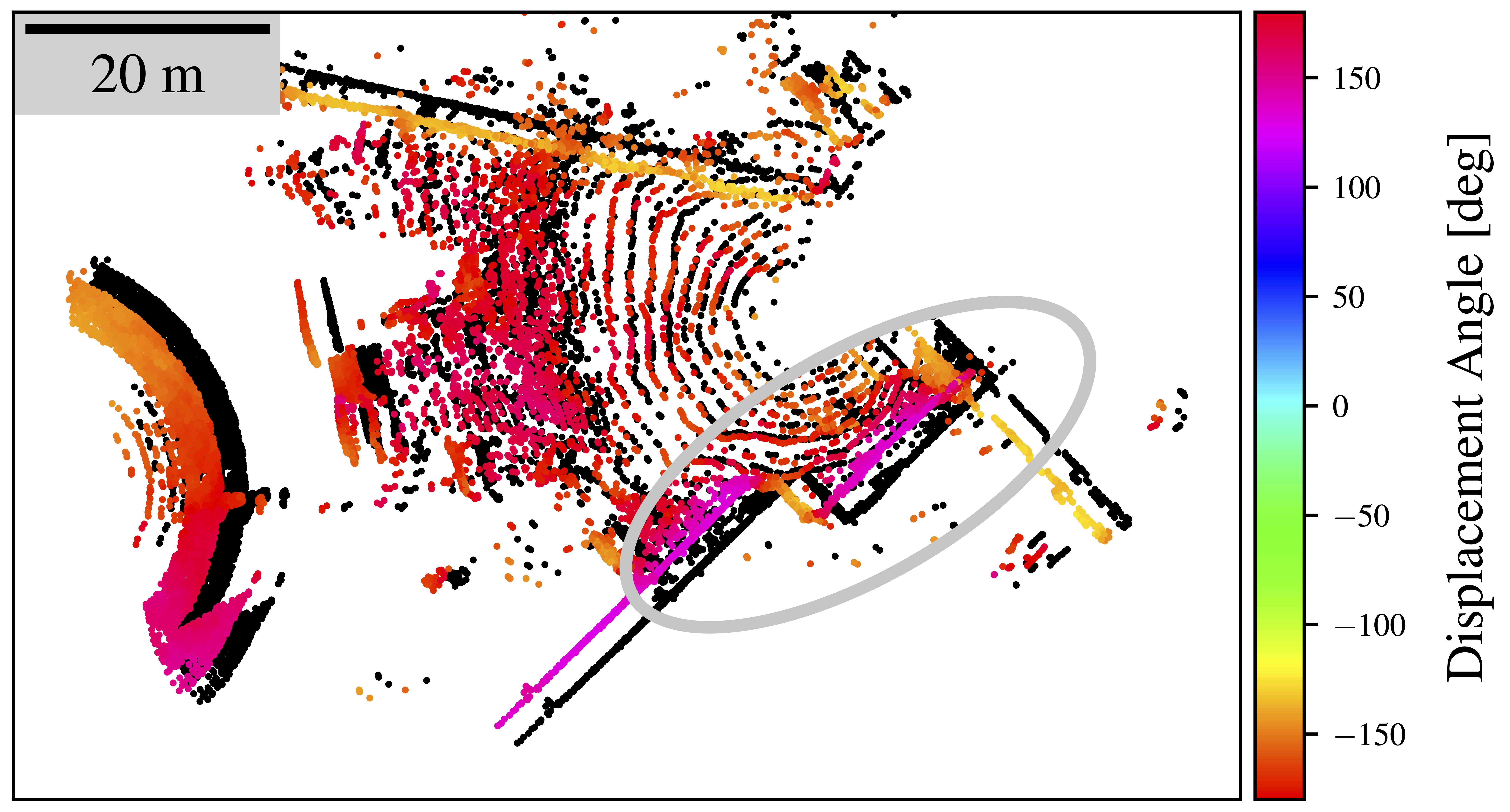
Figure 4: An example of the adversarial perturbations our model learns on the Boreas dataset. The adversarial point cloud generated by our model (coloured according to the angle of the displacement vector) is overlaid on top of the original point cloud (in black) for contrast. The linear features circled in grey are shifted in such a way that the features stay connected.

Examining the percentage of time ours is better than the baselines, we observe a decreasing trend as the perturbation bound increases. However, at the same time, the margin by which our method surpasses the baselines in mean pose error widens with bigger perturbation bounds.

IV-D3 Qualitative Example

Figure 4 provides a visual example of the kind of perturbation our model learns on the Boreas dataset. Our model shifts the point cloud in different directions and by different amounts. We observe that the rings at the center of the point cloud are not perturbed to the same extent as other geometric features. Regarding directions, most geometric features, such as the arc and the linear features, are translated largely in the direction of their normal vectors. Unlike the normal translation baseline that strictly moves points in the normal direction, our model exhibits a nuanced behavior. Specifically, for the linear features circled in grey, our model shifts them in directions slightly different from their normal vectors such that the features stay connected after perturbation.

IV-D4 Worst Pose Errors Over a Route

In this section, we study how the worst ICP pose errors estimated by our model vary over a route. We apply our model trained with $\lambda=2m$ to corrupt live scans collected over three Boreas repeat sequences that are over the same route but under different weather conditions. We plot the average induced translation pose errors at each location in Figure 5. Again, only longitudinal and lateral pose errors are considered. We notice that there are specific locations significantly more prone to attacks than others. At most locations, our model can induce less than 4 meters of pose errors in ICP. At locations coloured in red, our model can induce as much as 6 to 10 meters of pose errors. This is likely because some locations have very few landmarks upon which localization can rely. Prior work [9] pinpoints very similar dangerous spots in this trajectory and shows that these spots correspond to locations particularly vulnerable to corrupted measurements. Locations $a,b,d$, and $e$ in Figure 5 are examples of dangerous spots. All four locations are in the vicinity of parking lots, which provide very few landmarks for localization. Specifically, locations $a$ and $b$ are intersections in residential areas with small houses and a parking lot. Locations $d$ and $e$ have large parking lots on both sides of the road. In contrast, location $c$ that demonstrates high resilience to corruption in the measurements has a number of trees on both sides.

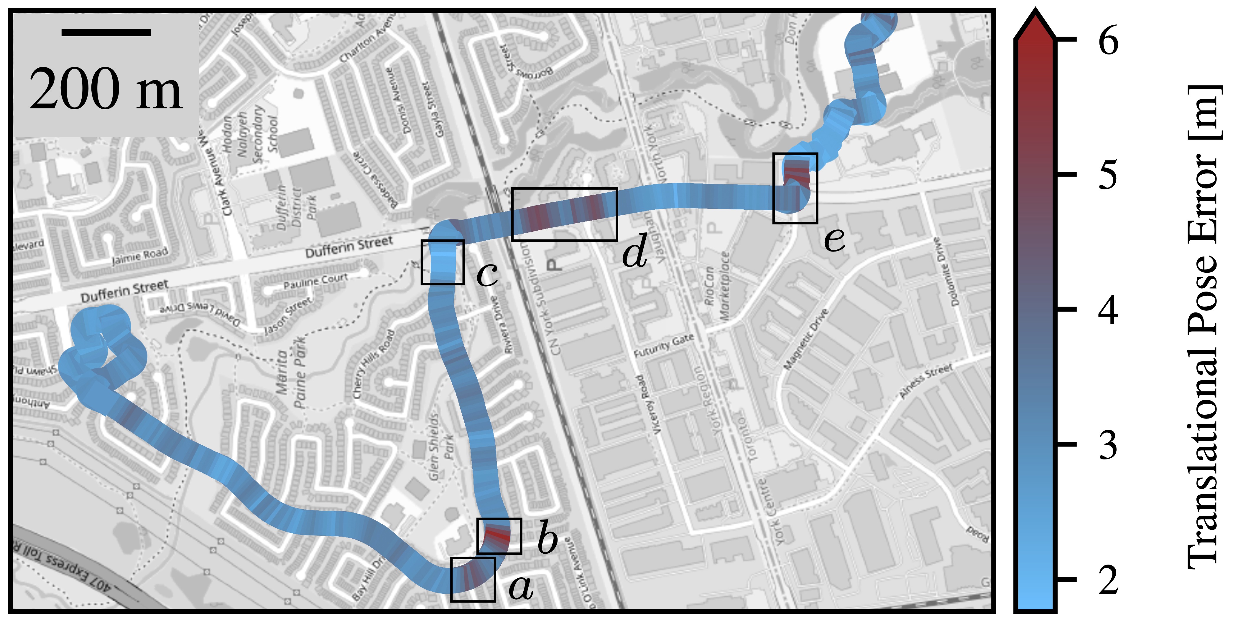
Figure 5: Worst-case translation pose errors over a route estimated by our model when allowed up to $\lambda=2m$ of perturbation. Locations are coloured based on the magnitude of their worst-case translation pose error. Errors are capped at 6 meters for better visualization. Some locations, such as $a,b,d,$ and $e$, are much more prone to attacks than others such as $c$.

V Conclusion

In this paper, we propose the first learning-based attack against the widely used lidar-based ICP algorithm. Our attack learns how to perturb a point cloud to maximize the pose error when using ICP to localize it against a map. Our attack successfully induces significant pose errors in ICP and consistently outperforms baselines across different perturbation bounds in more than 88% of cases. We also demonstrate the feasibility of using our attack to analyze the resilience of ICP and estimate the worst-case pose errors ICP may encounter during deployment, where challenging situations such as occlusions and adverse weather can cause unusually high pose errors. As an example application of our framework, we can identify certain locations along a route that have significantly higher worst-case pose errors than others, highlighting vulnerabilities of ICP.

For future work, we would like to explore other types of corruption such as point addition and removal to cover a wider range of possible scenarios a robot can encounter during deployment.

References

- [1] P.J. Besl and Neil D. McKay “A method for registration of 3-D shapes” In IEEE Transactions on Pattern Analysis and Machine Intelligence 14.2, 1992, pp. 239–256 DOI: 10.1109/34.121791
- [2] François Pomerleau, Francis Colas and Roland Siegwart “A Review of Point Cloud Registration Algorithms for Mobile Robotics”, 2015 DOI: 10.1561/2300000035
- [3] Huan Yin et al. “A Survey on Global LiDAR Localization: Challenges, Advances and Open Problems” In arXiv preprint arXiv:2302.07433, 2023
- [4] Clément Courcelle, Dominic Baril, François Pomerleau and Johann Laconte “On the Importance of Quantifying Visibility for Autonomous Vehicles under Extreme Precipitation” In Towards Human-Vehicle Harmonization 3, Intelligent Vehicles and Transportation, 2023, pp. 239–250 DOI: doi:10.1515/9783110981223-018
- [5] Yuki Endo, Ehsan Javanmardi and Shunsuke Kamijo “Analysis of Occlusion Effects for Map-Based Self-Localization in Urban Areas” In Sensors 21.15, 2021 DOI: 10.3390/s21155196
- [6] Keenan Burnett et al. “Boreas: A multi-season autonomous driving dataset” In The International Journal of Robotics Research 42.1-2, 2023, pp. 33–42 DOI: 10.1177/02783649231160195
- [7] Matthew Pitropov et al. “Canadian Adverse Driving Conditions dataset” In The International Journal of Robotics Research 40.4-5, 2020, pp. 681–690 DOI: 10.1177/0278364920979368
- [8] Keenan Burnett et al. “Are We Ready for Radar to Replace Lidar in All-Weather Mapping and Localization?” In IEEE Robotics and Automation Letters 7.4, 2022, pp. 10328–10335 DOI: 10.1109/LRA.2022.3192885
- [9] Johann Laconte, Daniil Lisus and Timothy D. Barfoot “Toward Certifying Maps for Safe Registration-Based Localization Under Adverse Conditions” In IEEE Robotics and Automation Letters 9.2, 2024, pp. 1572–1579 DOI: 10.1109/LRA.2023.3346751
- [10] Angel X. Chang et al. “ShapeNet: An Information-Rich 3D Model Repository” In arXiv preprint arXiv:1512.03012, 2015
- [11] Andrea Censi “An accurate closed-form estimate of ICP’s covariance” In Proceedings 2007 IEEE International Conference on Robotics and Automation, 2007, pp. 3167–3172 DOI: 10.1109/ROBOT.2007.363961
- [12] Turcan Tuna et al. “X-ICP: Localizability-Aware LiDAR Registration for Robust Localization in Extreme Environments” In IEEE Transactions on Robotics 40, 2024, pp. 452–471 DOI: 10.1109/TRO.2023.3335691
- [13] Ji Zhang, Michael Kaess and Sanjiv Singh “On degeneracy of optimization-based state estimation problems” In 2016 IEEE International Conference on Robotics and Automation (ICRA), 2016, pp. 809–816 DOI: 10.1109/ICRA.2016.7487211
- [14] Weikun Zhen and Sebastian Scherer “Estimating the Localizability in Tunnel-like Environments using LiDAR and UWB” In 2019 International Conference on Robotics and Automation (ICRA), 2019, pp. 4903–4908 DOI: 10.1109/ICRA.2019.8794167
- [15] Akshay Hinduja, Bing-Jui Ho and Michael Kaess “Degeneracy-Aware Factors with Applications to Underwater SLAM” In 2019 IEEE/RSJ International Conference on Intelligent Robots and Systems (IROS), 2019, pp. 1293–1299 DOI: 10.1109/IROS40897.2019.8968577
- [16] Maria Jokela, Matti Kutila and Pasi Pyykönen “Testing and Validation of Automotive Point-Cloud Sensors in Adverse Weather Conditions” In Applied Sciences 9, 2019, pp. 2341 DOI: 10.3390/app9112341
- [17] Jiancheng Yang et al. “Adversarial Attack and Defense on Point Sets” In arXiv preprint arXiv:1902.10899, 2019
- [18] Hang Zhou et al. “LG-GAN: Label Guided Adversarial Network for Flexible Targeted Attack of Point Cloud-based Deep Networks” In Proceedings of the IEEE/CVF Conference on Computer Vision and Pattern Recognition, 2020, pp. 10356–10365
- [19] Jiachen Sun, Yulong Cao, Qi Alfred Chen and Z. Morley Mao “Towards Robust LiDAR-based Perception in Autonomous Driving: General Black-box Adversarial Sensor Attack and Countermeasures” In Proceedings of the 29th USENIX Conference on Security Symposium, SEC’20 USA: USENIX Association, 2020
- [20] Q. Zhang et al. “On Adversarial Robustness of Trajectory Prediction for Autonomous Vehicles” In 2022 IEEE/CVF Conference on Computer Vision and Pattern Recognition (CVPR) Los Alamitos, CA, USA: IEEE Computer Society, 2022, pp. 15138–15147 DOI: 10.1109/CVPR52688.2022.01473
- [21] Wei Wang et al. “I Can See the Light: Attacks on Autonomous Vehicles Using Invisible Lights” In Proceedings of the 2021 ACM SIGSAC Conference on Computer and Communications Security, CCS ’21 New York, NY, USA: Association for Computing Machinery, 2021, pp. 1930–1944 DOI: 10.1145/3460120.3484766
- [22] Yuan Xu et al. “SoK: Rethinking Sensor Spoofing Attacks against Robotic Vehicles from a Systematic View” In 2023 IEEE 8th European Symposium on Security and Privacy (EuroS&P), 2023, pp. 1082–1100 DOI: 10.1109/EuroSP57164.2023.00067
- [23] Kota Yoshida, Masaya Hojo and Takeshi Fujino “Adversarial Scan Attack against Scan Matching Algorithm for Pose Estimation in LiDAR-Based SLAM” In IEICE Transactions on Fundamentals of Electronics, Communications and Computer Sciences E105.A.3, 2022, pp. 326–335 DOI: 10.1587/transfun.2021CIP0017
- [24] Charles R. Qi, Li Yi, Hao Su and Leonidas J. Guibas “PointNet++: Deep Hierarchical Feature Learning on Point Sets in a Metric Space” In Proceedings of the 31st International Conference on Neural Information Processing Systems, NIPS’17 Long Beach, California, USA: Curran Associates Inc., 2017, pp. 5105–5114
- [25] Daniil Lisus, Johann Laconte, Keenan Burnett and Timothy D. Barfoot “Pointing the Way: Refining Radar-Lidar Localization Using Learned ICP Weights” In arXiv preprint arXiv:2309.08731, 2023
- [26] Timothy D. Barfoot “State Estimation for Robotics”, 2023
- [27] Paul T Furgale and Timothy D. Barfoot “Visual Teach and Repeat for Long-Range Rover Autonomy” In Journal of Field Robotics, special issue on “Visual mapping and navigation outdoors”, 2010
- [28] Ilya Loshchilov and Frank Hutter “Decoupled Weight Decay Regularization” In 7th International Conference on Learning Representations, ICLR 2019, New Orleans, LA, USA, 2019 URL: https://openreview.net/forum?id=Bkg6RiCqY7