Dynamic clustering for heterophilic stochastic block models with time-varying node memberships

Abstract

We consider a time-ordered sequence of networks stemming from stochastic block models where nodes gradually change memberships over time and no network at any single time point contains sufficient signal strength to recover its community structure. To estimate the time-varying community structure, we develop KD-SoS (kernel debiased sum-of-square), a method performing spectral clustering after a debiased sum-of-squared aggregation of adjacency matrices. Our theory demonstrates via a novel bias-variance decomposition that KD-SoS achieves consistent community detection of each network even when heterophilic networks do not require smoothness in the time-varying dynamics of between-community connectivities. We also prove the identifiability of aligning community structures across time based on how rapidly nodes change communities, and develop a data-adaptive bandwidth tuning procedure for KD-SoS. We demonstrate the utility and advantages of KD-SoS through simulations and a novel analysis of the time-varying dynamics in gene coordination in the human developing brain system.

section Introduction

Longitudinal analyses of a network reveal insights into how communities of nodes are lost or created over time. Due to the complexity of most networks, statistical methods are necessary to uncover these broad dynamics. Simply put, suppose we observe a time-ordered sequence of networks among the same $n$ nodes represented as symmetric binary matrices $A^{(0)},\ldots,A^{(1)}\in\{0,1\}^{n\times n}$, where for time $t\in[0,1]$, the $(i,j)$-entry of $A^{(t)}$ denotes the presence or absence of interaction between two nodes at time $t$. Due to the non-Euclidean nature of the data, it is often difficult to assess if the larger-scale community structures changed over time and, if so, which specific nodes were changing communities at what rate. Sarkar & Moore (2006) developed one of the first methods to investigate these time-varying dynamics. However, research on the statistical properties of such estimators is recent by comparison (Han et al., 2015). See Kim et al. (2018); Pensky & Zhang (2019) for a comprehensive overview. Our goal in this paper is to provide a theoretically justifiable new method that is computationally efficient and can handle a wide range of network dynamics.

In this work, we focus on understanding the dynamics of gene coordination over human brain development, but our methods are applicable more broadly to investigate any time-ordered sequence of networks. Consider the single-cell RNA-seq (scRNA-seq) dataset initially published in Trevino et al. (2021), where the authors delineated a specific set of 18,160 cells representing how cycling progenitors (orange) develop into numerous types of maturing glutamatergics (shades of teal). The authors annotated these cells and discovered a set of 993 genes associated with their development. This data can be visualized through a UMAP (McInnes et al., 2018), a non-linear dimension-reduction method (Figure figureA). Using typical tools in the single-cell analysis toolbox such as Slingshot (Street et al., 2018), we can order the cells in this lineage from the youngest to oldest cells (Figure figureB) and visualize how the gene expression evolves across this lineage (Figure figureC). However, while this simple analysis shows apparent dynamics of the mean gene expression across pseudotime, the evolution of the gene coordination patterns is unknown. Do the genes tightly coordinated at the beginning of development remain tightly coordinated at the end of development, and are there tightly coordinated genes that are not highly expressed?

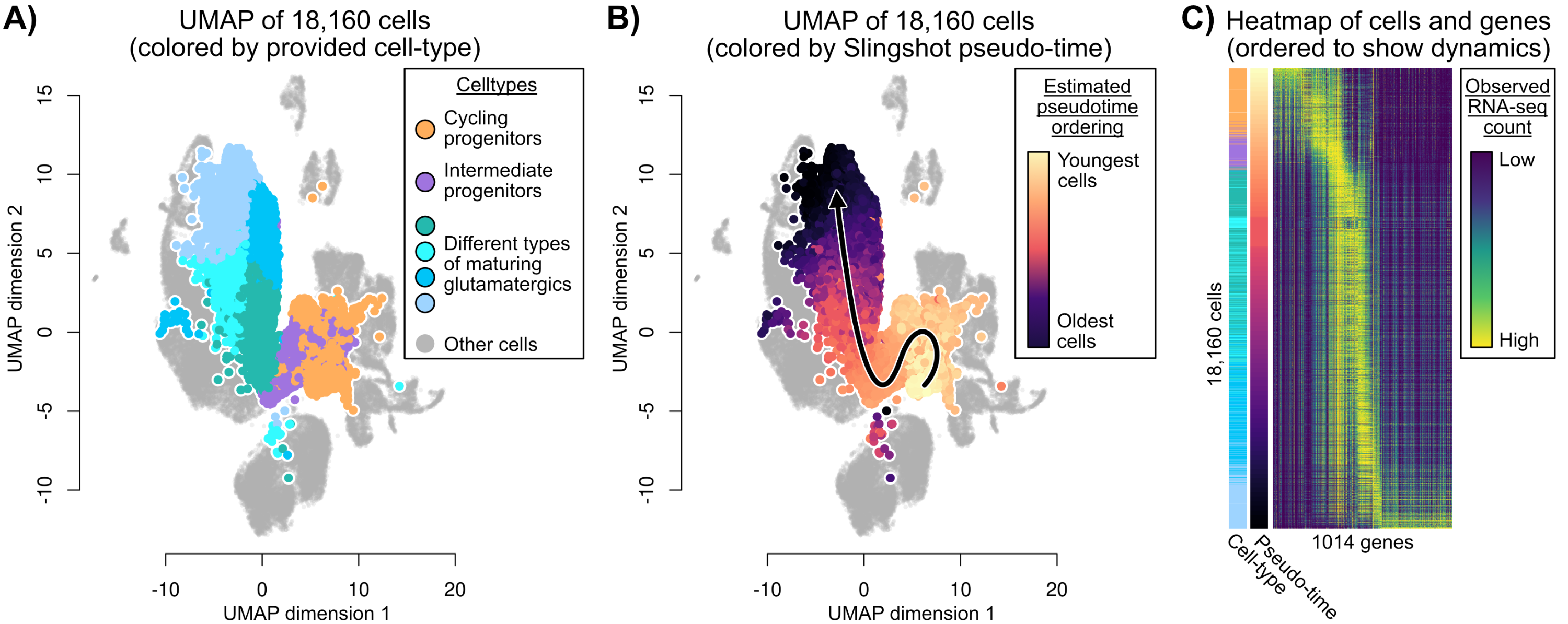
Figure figure: A) UMAP of the cells among the human developing brain, highlighting the 18,160 cells relevant to our analysis. These denotes cell types such as cycling progenitors (orange) and maturing glutamatergics (shades of teal). B) The 18,160 cells colored based on their estimated pseudotime using Slingshot (Street et al., 2018), colored from youngest (bright yellow) to oldest (dark purple). C) Heatmap ordering the cells based on their estimated pseudotime, and ordering the 993 relevant genes for this development. The gene expression for each cell is colored based on their expression (high as yellow, low as dark blue).

As reviewed in Kim et al. (2018), many statistical models exist for time-varying networks. This work focuses on time-varying stochastic block models (SBMs). SBMs (Holland et al., 1983) are a class of prototypical networks that reveal insightful theory while being flexible enough to model many networks in practice. Broadly speaking, an SBM represents each node as part of $K$ (unobserved) communities, and the presence of an edge between two nodes is determined solely by the nodes’ community label. Previous work has proven that there is a fundamental limit on how sparse the SBM can be before recovering the communities is impossible (Abbe, 2017). However, this fundamental limit could become even sparser when there is a collection of SBMs. This has led to many different lines of work. For example, one line of work studies the fixed community structure, where $T$ SBMs are observed with all the same community structure (Lei et al., 2020; Bhattacharyya & Chatterjee, 2020; Paul & Chen, 2020; Arroyo et al., 2021; Lei & Lin, 2022). A variant is that no temporal structure is imposed across the $T$ networks, but instead, each network slightly deviates from a common community structure at random (Chen et al., 2020). Another line of work is when $T$ time-ordered SBMs are observed, but there is a changepoint – all the networks before or all the networks after the changepoint share the same community structure (Liu et al., 2018; Wang et al., 2021).

Despite the abundance of aforementioned SBM models equipped with rigorous theory, they only partially apply to our intended analysis of the human developing brain. To provide the reader with a scope of the analysis, we plot the correlation network among the 993 genes for three different time points in Figure figure. These networks were constructed from 12 non-overlapping partitioning of cells across the estimated time, and we observe potentially gradual changes in community structure over time. See the Appendix for more details on the preprocessing. Hence, we turn towards time-varying SBM models, where the community structure changes slowly over time. To date, Pensky & Zhang (2019) and Keriven & Vaiter (2022) are among the only works that study this setting. This difficulty is induced by the simple observation that changes in community structure are discrete, which prevents typical non-parametric techniques from being easily applied. However, as discussed later, we take a different theoretical approach to analyze this problem and prove consistent estimation of each network’s community under broader assumptions. We briefly note that beyond time-varying SBMs, there are works on time-varying latent-position graphs (Gallagher et al., 2021; Athreya et al., 2022). Latent-position graphs are more general than SBMs, as they do not impose a community structure. In this work, we focus on SBMs as they are more applicable to understanding the gene coordination dynamics in the developing brain.

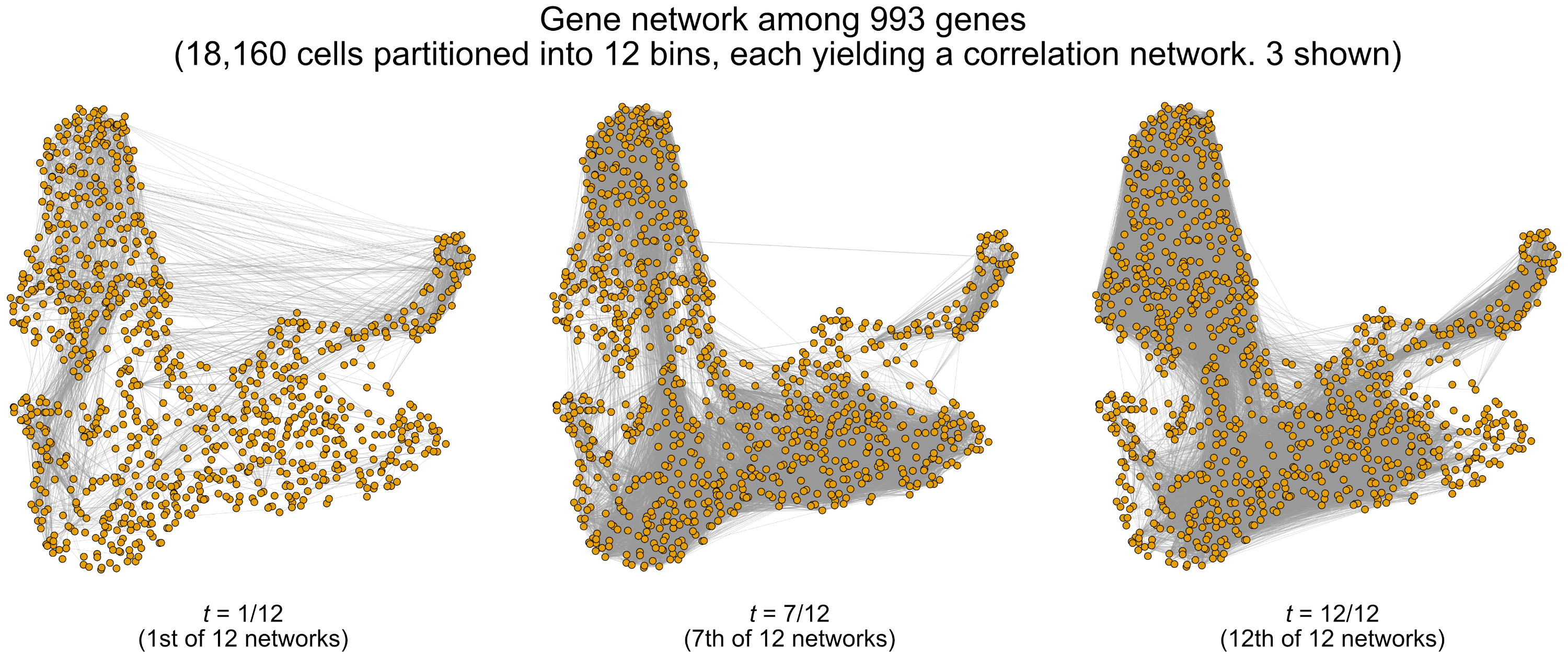
Figure figure: Three of twelve networks, for $t=1/12$ (i.e., gene network among the youngest cells), $t=7/12$ and $t=12/12$ (i.e., gene network among the oldest cells). These are constructed based on thresholding the correlation matrix among the 993 genes. The visual position of each gene is fixed for each network, but the edges among the gene varies.

The main contribution of this paper is a novel and computationally efficient method equipped with theoretical guarantees regarding community estimation in temporal SBMs with a time-varying community structure. Our method is inspired by Lei & Lin (2022), where a debiased sum-of-squared estimator was proven to estimate communities for fixed-community multi-layer networks consistently, allowing for both homophilic and heterophilic networks. We adapt this to the time-varying setting by introducing a kernel smoother and prove through a novel bias-variance decomposition that it can consistently estimate the time-varying communities, holding all other assumptions the same. In particular, while the nodes are gradually changing communities, we impose almost no conditions on the connectivity patterns except the positivity of the locally averaged squared connectivity matrix. We also formalize the information-theoretic relation between the number of networks and the rate nodes change communities as an identifiability condition.

Our second contribution is a tuning procedure for an appropriate kernel bandwidth that also does not impose restrictions on how the community relations change across networks. Leave-one-out tuning procedures designed in other matrix applications (Yang & Peng, 2020) where network $t$ is predicted using other temporally surrounding networks are inappropriate since these procedures require community relations to change smoothly over time. This also precludes Lepskii-based procedures (Pensky & Zhang, 2019). In contrast, our procedure is designed based on the cosine distance between eigenspaces – for network $t$, the cosine distance is computed between the eigenspaces of kernel-weighted networks for a time less than $t$ and of kernel-weighted networks for a time greater than $t$ respectively. The bandwidth that minimizes this distance averaged over all $t$ is deemed the most appropriate. We show through simulation studies and a thorough investigation of the scRNA-seq data that this procedure selects a desirable bandwidth.

section Dynamic stochastic block model

Let $n$ denote the number of nodes, and $m^{(0)}\in\{1,\ldots,K\}^{n}$ denote the initial membership vector, where $K$ is a fixed number of communities. That is, $m^{(0)}_{i}=k$ for $k\in\{1,\ldots,K\}$ if node $i$ starts in community $k$. We posit that each of the $n$ nodes changes communities according to a $\operatorname{{Poisson}}(\gamma)$ process with $\gamma>0$, independent of all other nodes. This means node $i\in\{1,\ldots,n\}$ changes communities at random times $0<x_{i,1}<x_{i,2}<\ldots<1$ where the expected difference between consecutive times is $1/\gamma$, and the node changes to one of the $K-1$ other communities with arbitrary probability. This process generates membership vectors $m^{(t)}$ for $t\in[0,1]$.

Although each node can potentially change communities multiple times throughout $t\in[0,1]$, we assume that only $T$ graphs at fixed time points are observed for

$$\mathcal{T}=\Big{\{}\frac{1}{T},\;\frac{2}{T},\;\ldots,\;1\Big{\}}.$$

The generative model for a specific graph $A^{(t)}\in\{0,1\}^{n\times n}$ for a time $t\in\mathcal{T}$ is as follows. Let $B^{(t)}\in[0,1]^{K\times K}$ be a symmetric matrix that denotes the connectivity matrix among the $K$ communities for a fixed positive integer $K$, and let $m^{(t)}$ be the random membership vector based on the above $\operatorname{{Poisson}}(\gamma)$ process. Each membership vector $m^{(t)}$ can be encoded as one-hot membership matrix $M^{(t)}\in\{0,1\}^{n\times K}$ where $M_{ik}^{(t)}=1$ if and only if node $i$ is in community $k$, and 0 otherwise. Then, the probability matrix $Q^{(t)}\in[0,1]^{n\times n}$ is defined as

$$Q^{(t)}=\rho_{n}\cdot M^{(t)}B^{(t)}\big{(}M^{(t)}\big{)}^{\top},$$ (equation)

for a network density parameter $\rho_{n}\in(0,1)$, and $P^{(t)}=Q^{(t)}-\operatorname{{diag}}(Q^{(t)})$. The observed graph $A^{(t)}$ for time $t\in\mathcal{T}$ is then sampled according to

$$A^{(t)}_{ij}=\begin{cases}\operatorname{{Bernoulli}}\big{(}P_{ij}^{(t)}\big{)},&\quad\text{if }i>j,\\ 0&\quad\text{if }i=j,\\ A^{(t)}_{ji}&\quad\text{otherwise}.\end{cases}$$ (equation)

This implies the following relation:

$$\mathbb{E}\big{[}A^{(t)}\big{]}=P^{(t)}=Q^{(t)}-\operatorname{{diag}}\big{(}Q^{(t)}\big{)}.$$

For two membership matrices $M$, $M^{\prime}$, define their confusion matrix $C(M,M^{\prime})$ as

$$C_{k\ell}(M,M^{\prime})=\Big{|}\big{\{}i\in\{1,\ldots,n\}:M_{ik}=1\text{ and }M^{\prime}_{i\ell}=1\big{\}}\Big{|}.$$ (equation)

Since the outputs of most clustering algorithms do not distinguish label permutations, to match the label permutation between $M$ and $M^{\prime}$, we solve the following assignment problem,

$$R(M,M^{\prime})=\arg\max_{R\in\mathbb{Q}_{K}}\big{\|}\operatorname{{diag}}(C(M,M^{\prime})R)\big{\|}_{1},$$ (equation)

where $\mathbb{Q}_{K}$ is the set of $K\times K$ permutation matrices. Equipped with $C(M,M^{\prime})$ and $R(M,M^{\prime})$, we define $L(M,M^{\prime})$ to be the relative Hamming distance between the two membership matrices $M$ and $M^{\prime}$,

$$L(M,M^{\prime})=1-\frac{1}{n}\big{\|}\operatorname{{diag}}(C(M,M^{\prime})R(M,M^{\prime})\|_{1}\,,$$ (equation)

or, in other words, the total proportion of mis-clustered nodes after optimal alignment. Furthermore, we define a square matrix $X\in\mathbb{R}^{K\times K}$ to be diagonally dominant if $X_{kk}\geq\sum_{\ell:\ell\neq k}|X_{k\ell}|$ for each $k\in\{1,\ldots,K\}$. If $C(M,M^{\prime})R(M,M^{\prime})$ and $C(M^{\prime},M)R(M^{\prime},M)$ are both diagonally dominant, we say that the two membership matrices $M,M^{\prime}$ as alignable. This means there is an unambiguous mapping of the $K$ communities in $M$ to those in $M^{\prime}$.

Our theoretical goal is to show the interplay between the number of nodes $n$, the number of observed networks $T$, community switching rate $\gamma$, and the network-sparsity parameter $\rho_{n}$ needed to estimate the $T$ membership matrices across time consistently. The existing theory of single-layer SBMs has already shown that if $\rho_{n}\gtrsim\log(n)$ for a single network, spectral clustering can asymptotically recover the community structure. At the same time, no method can achieve exact recovery if $\rho_{n}\lesssim\log(n)$ (Bickel & Chen, 2009; Lei & Rinaldo, 2015; Abbe, 2017). We are interested primarily in the latter setting, hoping the temporal structure can boost the signal for estimation. Some previous methods and theoretical analyses for this setting require strict assumptions on connectivity matrices $\{B^{(t)}\}$ (Pensky & Zhang, 2019; Keriven & Vaiter, 2022) – these matrices are required to vary across time smoothly and have strictly positive eigenvalues, i.e., cannot display patterns of heterophily where edges between communities are more frequent than edges within communities. We seek to develop a method that does not require these assumptions, extending the line of work in Lei et al. (2020); Lei & Lin (2022) to temporal SBMs with varying communities.

section Debiasing and kernel smoothing

section.subsection Estimator

Our estimator, the kernel debiased sum-of-squared (KD-SoS) spectral clustering, is motivated by Lei & Lin (2022), where we adopt using the de-biased sum of squared adjacency matrices to handle heterophilic networks. We describe our method using the box kernel for simplicity, but the method and theory can be extended to any kernels that are bounded, continuous, symmetric, non-negative and integrate to 1. The estimation procedure consists of two phases: individual time point smoothing and temporal aligning.

Provided a bandwidth $r\in[0,1]$ and a number of communities $K$, our estimator applies the following procedure for any $t\in\mathcal{T}$. First, compute the de-biased sum of squared adjacency matrices, where the summation is over all networks within a bandwidth $r$,

$$Z^{(t;r)}=\sum_{s\in\mathcal{S}(t;r)}\left[(A^{(s)})^{2}-D^{(s)}\right],\quad\text{where}\quad\mathcal{S}(t;r)=\mathcal{T}\cap[t-r,t+r],$$ (equation)

and $D^{(t)}\in\mathbb{R}^{n\times n}$ is the (random) diagonal matrix encoding the degrees of the $n$ nodes, i.e.,

$$\big{[}D^{(t)}\big{]}_{ii}=\sum_{j=1}^{n}A^{(t)}_{ij},\quad\text{for all }i\in\{1,\ldots,n\}.$$

Second, compute eigendecomposition of $\widehat{Z}^{(t;r)}$,

$$\widehat{Z}^{(t;r)}=\widehat{U}^{(t;r)}\widehat{\Lambda}^{(t;r)}(\widehat{U}^{(t;r)})^{\top},$$ (equation)

where the diagonal entries of $\widehat{\Lambda}^{(t;r)}$ are in descending order, and lastly, apply K-means clustering row-wise on the first $K$ columns of $\widehat{U}^{(t;r)}$. This yields the estimated memberships $\widetilde{m}^{(t)}\in\{1,\ldots,K\}^{n}$. This debiased sum-of-squared estimator is proven in Lei & Lin (2022) to consistently estimate communities under the fixed-community setting, where the squaring of adjacency matrices enable the population connectivity matrices $\{B^{(t)}\}$ to be semidefinite, and the debiasing corrects for the additive noise incurred by this squaring. This completes the estimation for each individual time point.

After estimating the communities for all $T$ time points, we align the estimated communities across time. Specifically, initialize $\widehat{M}^{(1/T)}$ as the one-hot membership matrix of $\widetilde{m}^{(1/T)}$. Let $\delta=1/T$. Then, suppose the aligned membership $\widehat{M}^{(t)}$ has been obtained, and we want to align the membership for $\widetilde{M}^{(t+\delta)}$, the one-hot membership matrix for $\widetilde{m}^{(t+\delta)}$. Define the confusion matrix

$$\widetilde{C}^{(t,t+\delta)}=C(\widehat{M}^{(t)},\widetilde{M}^{(t+\delta)})\,,$$ (equation)

according to the definition in (equation), and solve the following assignment problem,

$$\widehat{R}^{(t,t+\delta)}=R(\widehat{M}^{(t)},\widetilde{M}^{(t+\delta)})\,,$$ (equation)

according to (equation). This can be formulated as an Hungarian assignment problem, which can be solved via linear programming. Then, we align $\widetilde{M}^{(t+\delta)}$ with $\widehat{M}^{(t)}$ by using

$$\widehat{M}^{(t+\delta)}=\widetilde{M}^{(t+\delta)}\widehat{R}^{(t,t+\delta)}\,.$$

Let the estimated memberships for time $t$ to be $\widehat{m}^{(t)}$ where $\widehat{m}^{(t)}=k$ if and only if $\widetilde{m}^{(t)}=\ell$ and $\widehat{R}^{(t,t+\delta)}_{\ell k}=1$. Finally, we return the final estimated memberships $\widehat{m}^{(t)}$ for $t\in\mathcal{T}$.

Optionally, we can compute if $\widetilde{C}^{(t,t+\delta)}\widehat{R}^{(t,t+\delta)}$ and $(\widetilde{C}^{(t,t+\delta)}\widehat{R}^{(t,t+\delta)})^{\top}$ are both diagonally dominant for all $t\in\mathcal{T}\backslash\{1\}$. If so, we say that the entire sequence of communities in $\mathcal{T}$ is alignable, which means we can track the evolution of specific nodes and communities across time.

section.subsection Bias-variance tradeoff for spectral clustering

We first describe the bias-variance decomposition foundational to our work. Let $n_{1}^{(t)},\ldots,n_{K}^{(t)}$ denote the number of nodes in each community at time $t$, and $n_{\min}^{(t)}=\min\{n^{(t)}_{1},\ldots,n_{K}^{(t)}\}$. Let $\Delta^{(t)}\in\mathbb{R}^{K\times K}$ denote the diagonal matrix where

$$\operatorname{{diag}}\big{(}\Delta^{(t)}\big{)}=\big{\{}n_{1}^{(t)},\ldots,n_{K}^{(t)}\big{\}}.$$

Let $\Pi^{(t)}=M^{(t)}(\Delta^{(t)})^{-1}M^{(t)})^{\top}$ be the projection matrix of the column subspace of $M^{(t)}$. Additionally, define the noise matrix $X^{(t)}=P^{(t)}-A^{(t)}$. Observe the following bias-variance decomposition.

Lemma section.theorem.

Given the model in Section section, the following deterministic equality holds,

$$\sum_{s\in\mathcal{S}(t;r)}(A^{(s)})^{2}-D^{(s)}=\underbrace{\Big{[}\sum_{s\in\mathcal{S}(t;r)}(Q^{(s)})^{2}-\Pi^{(t)}(Q^{(s)})^{2}\Pi^{(t)}\Big{]}}_{I}$$ (equation)

$$\qquad+\underbrace{\Big{[}\sum_{s\in\mathcal{S}(t;r)}\big{[}\operatorname{{diag}}(Q^{(t)})\big{]}^{2}-Q^{(t)}\operatorname{{diag}}(Q^{(t)})-\operatorname{{diag}}(Q^{(t)})Q^{(t)}\Big{]}}_{II}$$

$$\qquad+\underbrace{\Big{[}\sum_{s\in\mathcal{S}(t;r)}X^{(s)}P^{(s)}+P^{(s)}X^{(s)}\Big{]}}_{III}+\underbrace{\Big{[}\sum_{s\in\mathcal{S}(t;r)}(X^{(s)})^{2}-D^{(s)}\Big{]}}_{IV}$$

$$\qquad+\underbrace{\Big{[}\sum_{s\in\mathcal{S}(t;r)}\Pi^{(t)}(Q^{(s)})^{2}\Pi^{(t)}\Big{]}}_{V}.$$

We deem this decomposition as the bias-variance decomposition for dynamic SBMs since term $I$ represents the deterministic bias dictated by nodes changing communities, term $II$ represents the deterministic diagonal bias, term $III$ represents a random error term centered around 0, term $IV$ represents the random variance term, and term $V$ represents the deterministic signal matrix containing the community information. We note that this decomposition differs from those used in Pensky & Zhang (2019) and Keriven & Vaiter (2022), which instead yield a decomposition that requires smoothness assumptions in $\{B^{(t)}\}$ to derive community-consistency.

section.subsection Consistency of time-varying communities

In the following, we discuss the assumptions and theoretical guarantees for KD-SoS. We define the following notation. For two sequences $a_{n}$ and $b_{n}$, we define $a_{n}=O(b_{n})$, $a_{n}=o(b_{n})$, and $a_{n}=\omega(b_{n})$ to denote $a_{n}$ is asymptotically bounded above by $b_{n}$ by a constant, $\lim a_{n}/b_{n}=0$, or $\lim a_{n}/b_{n}=\infty$ respectively. For a symmetric matrix $X$, let $\lambda_{\min}(X)$ denote its smallest eigenvalue in absolute value.

[Asymptotic regime] Assume a sequence where $n$ and $T$ are increasing, $n,T\geq 3$, and $T\log(T)/n=o(1)$. Additionally, $\rho_{n}$ and $\gamma$ can vary with $n$ and $T$, but there exists a constant $c_{1}$ such that $n\rho_{n}\leq c_{1}$. Furthermore, assume $K$ is fixed.

We codify the membership dynamics described in Section section with the following assumption. [Independent Poisson community changing rate] Assume for a given community switching rate $\gamma\geq 0$, each node changes memberships at random times between $t\in[0,1]$ according to a $\operatorname{{Poisson}}(\gamma)$ process, independent of all other nodes.

[Stable community sizes] Assume that across all $t\in[0,1]$ and all communities $k\in\{1,\ldots,K\}$, there exists a constant $c_{2}$ independent of $n,T,\gamma,\rho_{n}$ satisfying $1\leq c_{2}$ such that

$$\mathbb{P}\left\{n_{k}^{(t)}\in\Big{[}\frac{1}{c_{2}K}\cdot n,\;\frac{c_{2}}{K}\cdot n\Big{]},\quad\text{for all }k\in\{1,\ldots,K\},\;t\in\mathcal{T}\right\}\geq 1-\epsilon_{c_{2},n}.$$

for some $\epsilon_{c_{2},n}\rightarrow 0$.

[Minimum eigenvalue of aggregated connectivity matrix] Assume that the sequence $\{B^{(t)}\}$ from $t\in[0,1]$ is fixed and is an integrable process across each $(i,j)\in\{1,\ldots,K\}^{2}$ coordinate. Additionally, for a chosen $\delta>0$, we define

$$c_{\delta}=\min_{\begin{subarray}{c}t_{1},t_{2}\in[0,1],\\ t_{2}-t_{1}\geq 2\delta\end{subarray}}\lambda_{\min}\Big{(}\frac{1}{t_{2}-t_{1}}\int_{s=t_{1}}^{t_{2}}(B^{(s)})^{2}ds\Big{)}\geq 0.$$

[Alignability] Assume that along the sequence of $\gamma$ and $T$,

$$\gamma/T=o(1).$$ (equation)

Remark section.theorem (Additional remark for Assumption section.subsection).

Assumption section.subsection extends the balanced community size condition from a single time point to a uniform version across all time points. It serves two purposes: First, this condition is needed to control the error bound in each single time point. Second, when combined with Assumption section.subsection, it guarantees alignability of estimated communities across time. The exact relationship between $c_{2}$ and $\epsilon_{c_{2},n}$ depends on the switching rate $\gamma$, as well as the transition probabilities between communities when a node changes membership. This assumption precludes the scenario where some communities vanish as nodes are more likely to move out than move in. Under certain common conditions of the transition probabilities, such as mixing, Assumption section.subsection can hold using concentration inequalities and union bound. We provide a concrete example in Section section.subsection below.

Remark section.theorem (Additional remark for Assumption section.subsection).

Assumption section.subsection states that column space of the matrices $\{(B^{(t)})^{2}\}$ should span enough of $\mathbb{R}^{K}$ in an average sense among all $t\in[t_{1},t_{2}]$. That is, $B^{(t)}$ can be rank deficient for any particular $t\in[t_{1},t_{2}]$, but as long as $\delta$ is large enough, the average of $\{(B^{(t)})^{2}\}$ is full rank. As we will discuss later, $c_{\delta}$ has a nuanced relation with our bandwidth $r$ and the consistency of our estimator – estimating the community structure consistently for each time $t$ will be difficult if we choose a bandwidth $r=\delta$ where $c_{\delta}\approx 0$.

Remark section.theorem (Additional remark for Assumption section.subsection).

As we will show later in Section section.subsection, Assumption section.subsection is a label permutation identifiability assumption. Without it, KD-SoS can still estimate each network’s community structure. However, it would be difficult to align the communities across time, where “alignablility” will be defined later as the main focus of Section section.subsection. Recall that since each node changes memberships independently of one another according to the Poisson($\lambda$) process, the expected number of nodes to change memberships within a time interval of $1/T$ (i.e., the time elapsed between two consecutively observed networks) is roughly $n\gamma/T$ if $\gamma/T\lesssim 1$. Combined with Assumption section.subsection, a more explicit equivalent statement of (equation) is

$$n\gamma/T=o(n/K).$$

This demonstrates the intuition that the networks’ communities are alignable across time if the number of changes between consecutive networks is less than the smallest community size.

Provided these assumptions, KD-SoS’s estimated communities have the following pointwise relative Hamming estimation error for the network at time $t\in\mathcal{T}$. Let the function $(x)_{+}$ denote $\min\{0,x\}$.

Theorem section.theorem.

Given Assumptions section.subsection, section.subsection, section.subsection, and section.subsection for the model in Section section, or a bandwidth $r\in[0,1]$ satisfying $(rT+1)^{1/2}n\rho_{n}\geq c_{3}\log^{1/2}(rT+n+1)$ for some constant $c_{3}>1$, then at any particular $t\in\mathcal{T}$,

$$L\big{(}G^{(t)},\widehat{G}^{(t)}\big{)}\leq c\cdot\frac{1}{(1-(\gamma r+\log(n)/n)^{1/2})^{2}_{+}}\cdot\Big{(}\gamma r+\frac{\log(n)}{n}+\frac{1}{n^{2}}+\frac{\log(rT+n)}{rTn^{2}\rho_{n}^{2}}\Big{)},$$ (equation)

with probability at least $1-O((rT+n)^{-1})-\epsilon_{c_{2},n}$ for some constant $c>0$ that depends on $c_{1}$, $c_{2}$, $c_{3}$, $c_{\delta}$, and $K$.

Observe that if $\gamma r$ is close to 1 or larger, then our bound in Theorem section.theorem is vacuously true since $L(G^{(t)},\widehat{G}^{(t)})$ has to be less than 1, see (equation). Notably, Assumption section.subsection is not needed to estimate the community structure of a particular network consistently, but we discuss its importance in the next section.

Remark section.theorem (Explicit relation between $r$ and minimal eigenvalue in Assumption section.subsection).

We expand upon Remark section.theorem. In Theorem section.theorem, we had stated the bandwidth $r$ distinctly from the bandwidth $\delta$ used to define the minimum eigenvalue $c_{\delta}$ stated in Assumption section.subsection for simplicity of exposition. We can derive a similar theorem where both bandwidths are the same, i.e., $r=\delta$. This is because the minimum eigenvalue $c_{\delta}$ only appears in the denominator when applying Davis-Kahan. Hence, we can rewrite RHS of (equation) to explicitly include the dependency on $c_{\delta}$, which would result in an upper bound proportional to

$$\frac{1}{c_{\delta}^{2}\cdot(1-(\gamma r+\log(n)/n)^{1/2})^{2}_{+}}\cdot\Big{(}\gamma r+\frac{\log(n)}{n}+\frac{1}{n^{2}}+\frac{\log(rT+n)}{rTn^{2}\rho_{n}^{2}}\Big{)}.$$

If $c_{\delta}=0$, the above equation would equal infinity, yielding a vacuously true upper bound.

We now derive an upper bound for the relative Hamming error when we use the near-optimal bandwidth $r$.

Corollary section.theorem (Near-optimal bandwidth).

Consider the setting in Theorem section.theorem with the bandwidth

$$r^{*}=\min\Big{\{}c\cdot\frac{1}{(\gamma T)^{1/2}n\rho_{n}},1\Big{\}},$$

for some constant $c>0$ that depends on $c_{1}$, $c_{2}$, $c_{3}$, $c_{\delta}$, and $K$. If the asymptotic setting satisfies

$$\gamma r^{*}=\sqrt{\frac{\gamma}{T}}\cdot\frac{1}{n\rho_{n}}\ll 1,$$

then the bandwidth $r^{*}$ minimizes the rate in Theorem section.theorem up to logarithmic factors.

Observe that $r^{*}$ in Corollary section.theorem captures an intuitive behavior. If the number of nodes $n$ or network density $\rho_{n}$ increases, then there is more signal in each network, reducing the bandwidth $r^{*}$. If the community switching rate $\gamma$ increases, there is less incentive to aggregate across networks, reducing $r^{*}$. Loosely speaking, observe that box kernel roughly averages over $O(r^{*}T)$ networks, meaning that the number of networks relevant for computing the community structure of network $t$ is approximately $O(\sqrt{T})$ networks if $\gamma$ and $n\rho_{n}$ (the expected number of edges per node) are held constant. This means the bandwidth grows slower than the total number of networks $T$, which is reasonable. Next, we state the resulting relative Hamming error stemming from this choice of bandwidth $r^{*}$. In particular, we are interested in two regimes based on whether $r^{*}\rightarrow 1$ (i.e., averaging across all $T$ networks asymptotically) or $r^{*}\rightarrow 0$ (i.e., averaging across a smaller and smaller proportion of the $T$ networks asymptotically).

Corollary section.theorem (Slow community-changing regime).

Given Assumptions section.subsection, section.subsection, section.subsection, and section.subsection for the model in Section section, and bandwidth $r^{*}$ defined in Corollary section.theorem, consider an asymptotic sequence of $\{n,T,\gamma,\rho_{n}\}$ where

$$\gamma\rightarrow 0,\quad\text{and}\quad T^{1/2}n\rho_{n}=\omega\big{(}\log^{1/2}(T+n)\big{)}.$$ (equation)

In this setting, $r^{*}\rightarrow 1$ and KD-SoS has a relative Hamming error of

$$L\Big{(}G^{(t)},\widehat{G}^{(t)}\Big{)}=O\Big{(}\gamma+\frac{\log(n)}{n}+\frac{1}{n^{2}}+\frac{\log(T+n)}{T(n\rho_{n})^{2}}\Big{)}\rightarrow 0,$$

with probability $1-O((T+n)^{-1})$ for any particular $t\in\mathcal{T}$.

Corollary section.theorem (Fast community-changing regime).

Given Assumptions section.subsection, section.subsection, section.subsection, and section.subsection, for the model in Section section, and bandwidth $r^{*}$ defined in Corollary section.theorem, consider an asymptotic sequence of $\{n,T,\gamma,\rho_{n}\}$ where

$$\gamma=\omega(1)\,,\quad\text{and}\quad\gamma=o\Big{(}\frac{T(n\rho_{n})^{2}}{\log(T+n)}\Big{)}.$$ (equation)

In this setting, $r^{*}\rightarrow 0$ and KD-SoS has a relative Hamming error of

$$L\Big{(}G^{(t)},\widehat{G}^{(t)}\Big{)}=O\Big{(}\frac{\gamma^{1/2}}{T^{1/2}n\rho_{n}}+\frac{\log(n)}{n}+\frac{1}{n^{2}}+\frac{\gamma^{1/2}\log\big{(}T^{1/2}/(\gamma^{1/2}n\rho_{n})+n\big{)}}{T^{1/2}n\rho_{n}}\Big{)}\rightarrow 0,$$

with probability $1-O((T+n)^{-1})$ for any particular $t\in\mathcal{T}$.

Observe that the two conditions (equation) and (equation) dichotomize the settings in a “slow community switching regime” and a “fast community switching regime” respectively. In the former setting, the nodes become less likely to change communities along the asymptotic sequence of $\{n,T,\gamma,\rho_{n}\}$, eventually resulting in KD-SoS averaging over all $T$ networks. In this regime Corollary section.theorem concurs with the recent results in static multi-layer SBM (Lei et al., 2020; Lei & Lin, 2022; Lei et al., 2023), which imply that $T^{1/2}n\rho_{n}\gg\log^{1/2}(T+n)$ is nearly necessary, up to logarithm factors, for consistent community estimation. In the latter setting, the bandwidth converges to 0 due to the nodes changing communities too quickly relative to the other parameters $T$, $n$, and $\rho_{n}$. Observe that if $n\rho_{n}=\log^{1/2}(T+n)$, then (equation) is equivalent to $\gamma/T=o(1)$, which is the requirement posed in Assumption section.subsection. This further upper-bounds how often nodes can change communities relative to the total number of networks $T$. As we will show in the next section, though, this requirement is not just for consistent estimation of a network’s community structure but also for ensuring the alignability of the communities across the $T$ networks.

section.subsection Identifiability bound for aligning communities across time

While Theorem section.theorem proves consistent estimation of the community structure at each time $t$, we now turn our attention towards proving that estimated community structure at each time $t$ can be aligned to those at the previous time $s=t-1/T$. This is an important but separate concern from the consistency proven in Theorem section.theorem since we strive to track how individual communities evolve over time. Our estimator uses the Hungarian assignment (equation) to align communities across time since the K-mean clusterings return unordered memberships. For this section, we will work under the pretense that for a sequence of membership matrices $M^{(1/T)},M^{(2/T)},\ldots,M^{(1)}$, we have already applied Hungarian assignment to each consecutive pair of membership matrices to optimally permute the column order. Our discussion of alignability here will show that even after this column permutation, there could still be detrimental ambiguity on how to track individual communities over time. As alluded to in Section section.subsection, we prove how alignability of communities across time is related to Assumption section.subsection. We define it formally below.

Definition section.theorem (Alignability of memberships across time).

Let $M^{(1/T)}$, $M^{(2/T)}$, $\ldots,~{}M^{(1)}$ denote $T$ membership matrices. We say the sequence of memberships are alignable if

$$C(M^{(t)},M^{(t+1/T)})\quad\text{and}\quad\big{(}C(M^{(t+1/T)},M^{(t)})\big{)}\quad\text{are both diagonally dominant}$$

for all $t\in\{1/T,2/T,\ldots,(T-1)/T\}$, where the confusion matrices $C(M^{(t)},M^{(t+1/T)})$ are defined in (equation).

We view $M^{(1/T)},M^{(2/T)},\ldots,M^{(1)}$ as the “true” membership matrices that encode the time-varying community structure that we wish to estimate, even though these are technically random matrices. From the data-generative point of view, alignability implies that $R^{(t,t+1/T)}=I_{K}$ defined in (equation) for all $t$. Indeed, for times $t$ and $t+1/T$, if the optimal assignment between the unobserved communities $M^{(t)}$ and $M^{(t+1/T)}$ is not the identity, then there is no hope of recovering the alignment of the estimated communities consistently. Hence, intuitively, alignability requires that nodes do not switch memberships too quickly, relative to the amount of time between consecutive networks, $1/T$.

Below, we first prove that when $\gamma$ is in a regime that violates Assumption section.subsection, there always exists a non-vanishing probability that $T$ networks can not be aligned. Later, we prove that when $\gamma$ is in a regime that satisfies Assumption section.subsection for specifically a two-community model, then all $T$ networks are alignability with high probability. Since tracking the community sizes over time under Assumption section.subsection involves specifying the transition probabilities and the number of times such transition occurs in a single time interval, to simplify the discussion in this subsection, we will consider an alternative discrete approximation of Assumption section.subsection.

[Discrete approximation of Assumption section.subsection] For each $t\in\mathcal{T}\backslash\{1\}$, each node changes its community membership from time $t$ to $t+1/T$ independently with probability $\gamma/T$.

Proposition section.theorem (Lack of alignability).

Given Assumptions section.subsection and section.theorem for the model in Section section, if

$$\gamma\geq T\cdot\log\bigg{[}\bigg{(}1-\frac{1}{2}\cdot\Big{(}\frac{(2n)^{1/2}}{T-1}\Big{)}^{1/n}\bigg{)}^{-1}\bigg{]},$$

then the probability that the set of random membership matrices $M^{(1/T)},M^{(2/T)},\ldots,M^{(1)}$ is not alignable is strictly bounded away from 0.

Observe that as $n$ and $T$ tend to infinity, the relation in Proposition section.theorem simplifies to

$$\gamma\geq T\cdot\log(2)\approx T\cdot 0.693,$$

and when $\gamma/T=0.693$, each node has roughly a 50% probability of switching communities between each consecutive pair of observed networks.

The proof of the lack of alignability first revolves around the observation that if more than $n/2$ nodes change memberships between consecutive times $t$ and $t+1/T$, i.e.,

$$\big{\|}M^{(t)}-M^{(t+1/T)}\big{\|}_{0}>n,$$ (equation)

where $\|x\|_{0}$ denotes the number of non-zero elements in $x$, then, deterministically, the Hungarian assignment between the unobserved membership matrices $M^{(t)}$ and $M^{(t+1/T)}$ will not be the identity matrix. This means the two membership matrices are not alignable. The proof shows that the event (equation) occurs with non-vanishing probability.

In contrast, to show that $\gamma/T=o(1)$ ensures alignability, our proof strategy is more delicate, as we need to ensure alignability between time $t$ and $t+1/T$ for each $t\in\mathcal{T}\backslash\{1\}$. First, we discuss a deterministic condition that ensures alignability among all the community structures.

Proposition section.theorem (Deterministic condition for alignability).

Assume any fixed sequence of membership matrices $M^{(1/T)},M^{(2/T)},\ldots,M^{(1)}$. For this sequence, if the number of nodes that change memberships between time $t$ and $t+1/T$ is less than half of the smallest community size at time $t$ for each pair of consecutive time points, meaning

$$\big{\|}M^{(t)}-M^{(t+1/T)}\big{\|}_{0}<\min_{k\in\{1,\ldots,K\}}\sum_{i=1}^{n}M^{(t)}_{ik},\quad\text{for some time }t\in\mathcal{T}\backslash\{1\},$$

then deterministically this sequence of matrices $M^{(1/T)},M^{(2/T)},\ldots,M^{(1)}$ is alignable.

Proposition section.theorem highlights that alignability is guaranteed if not many nodes change communities relative to the smallest community size. Next, the following proposition ensures that if $\gamma/T=o(1)$, this event occurs with high probability, where we focus specifically on a two-community model (i.e., $K=2$), where each community starts with equal sizes.

Proposition section.theorem (Alignability in a two-community model).

Given Assumptions section.subsection, section.subsection, and section.theorem for the model in Section section for a two-community model (i.e., $K=2$) initialized at $t=0$ to have equal community sizes, if $\gamma/T=o(1)$, then with probability at least $1-2/T$, the set of random membership matrices $M^{(1/T)},M^{(2/T)},\ldots,M^{(1)}$ is alignable.

This proof involves a novel recursive martingale argument since we need to ensure that alignability holds for the entire sequence of membership matrices across each pair of consecutive time points. We expect the argument to work for more general settings under mild conditions with more careful bookkeeping.

section Numerical experiments

In this section, we describe the tuning procedure to choose $r$ in a data-adaptive manner since the optimal bandwidth in Corollary section.theorem involves nuisance parameters. Our simulations demonstrate that 1) the tuning procedure reflects the oracle bandwidth, and 2) KD-SoS and the tuning procedure combined outperform other estimators for time-varying SBMs.

section.subsection Tuning procedure

We design the following procedure to tune the bandwidth $r$ in practice. Observe that typical tuning procedures for time-varying scalar or matrix-valued data often rely on the observed data’s local smoothness across time. For example, this may be predicting the network $A^{(t)}$ using all other networks $\{A^{(s)}\}$ for $s\in\mathcal{S}(t;r)\backslash\{t\}$ for $\mathcal{S}(t;r)$ defined in (equation), but such a procedure would necessarily require additional smoothness assumptions on the connectivity matrices $\{B^{(t)}\}$ on top of our weaker integrability assumption in Assumption section.subsection. Since our estimation theory in Theorem section.theorem does not require these additional assumptions, we seek to design a tuning procedure that also does not.

Recall that while Theorem section.theorem does not require smoothness across $\{B^{(t)}\}$, we assume that the community structure is gradually changing via a Poisson($\gamma$) process where $\gamma/T=o(1)$ (Assumption section.subsection). Our theory also demonstrates that changes to the community structure are reflected in the eigenspaces of the probability matrices $\{P^{(t)}\}$. This inspires our method – for a particular time $t\in\mathcal{T}$ and choice of bandwidth $r$, we kernel-average the networks earlier than $t$ (i.e., $\{A^{(s)}\}$ for $s<t$) and compute its leading eigenspace. We then compute the $\sin\theta$ distance (defined below) of this eigenspace from the kernel-average the networks later than $t$ (i.e., $\{A^{(s)}\}$ for $s>t$). A small $\sin\Theta$ distance for an appropriate choice of the bandwidth $\widehat{r}$ would be indicative of two aspects, relative to other choices of $r$: 1) the community structure among the networks in $\mathcal{S}(t;\widehat{r})\backslash[0,t)$ are not too dissimilar to those in networks in $\mathcal{S}(t;\widehat{r})\backslash(t,1]$, and 2) $\widehat{r}$ is large enough to produce stably estimated eigenspaces among the networks in $\mathcal{S}(t;\widehat{r})\backslash[0,t)$ or $\mathcal{S}(t;\widehat{r})\backslash(t,1]$. Reflecting on our bias-variance decomposition in (equation), the first regards the bias caused by community dynamics, and the second regards the variance due to sparsely observed networks.

Recall that for two orthonormal matrices $U,V\in[-1,1]^{n\times K}$, the $\sin\Theta$ distance (measured via Frobenius norm) is defined as,

$$\big{\|}\sin\Theta(U,V)\big{\|}_{F}=\sqrt{K-\big{\|}U^{\top}V\big{\|}^{2}_{F}}.$$ (equation)

(See references such as Stewart & Sun (1990) and Cai et al. (2018).) Formally, our procedure is as follows. Suppose a grid possible bandwidths $r_{1},\ldots,r_{m}$ are provided, in addition to the observed networks $\{A^{(t)}\}$.

1. For each bandwidth $r\in\{r_{1},\ldots,r_{m}\}$, compute the score of the bandwidth $\theta(r)$ in the following way.

   1. For each time $t\in\mathcal{T}$, compute the leading eigenspaces of $\sum_{s\in\mathcal{S}}(A^{(s)})^{2}-D^{(s)}$, where $\mathcal{S}$ is either $\mathcal{S}(t;c\cdot r)\backslash[0,t)$ or $\mathcal{S}(t;c\cdot r)\backslash(t,1]$ for $\mathcal{S}(t;c\cdot r)$ defined in (equation). Then, compute the $\sin\Theta$ distance between these two eigenspaces via (equation), denoted as $\theta(t;r)$.

   2. Average $\theta(t;r)$ over $t$. That is, $\theta(r)=\sum_{t}\theta(t;r)/T$.

2. Choose the optimal bandwidth with the smallest score, i.e., $\widehat{r}=\operatorname*{arg\,min}_{r\in\{r_{1},\ldots,r_{m}\}}\theta(r)$.

Observe the presence of a small adjustment factor $c>0$ when deploying the above tuning strategy. This is to account for the fact the size of the sets $\mathcal{S}(t;c\cdot r)\backslash[0,t)$ and $\mathcal{S}(t;c\cdot r)\backslash(t,1]$ are both roughly $c\cdot rT$, while the usage of $\widehat{r}$ in KD-SoS would use $\mathcal{S}(t;\widehat{r})$, a set of size roughly $2\cdot\widehat{r}T+1$. Hence, the adjustment factor $c$ scales the bandwidths when tuning to reflect its performance when used by KD-SoS. We have found $c=2$ to be a reasonable choice in practice.

section.subsection Simulation

We provide numerical experiments that demonstrate that our estimator described in Section section.subsection is equipped with a tuning procedure which: 1) selects the bandwidth based on data that mimics the oracle that minimizes the Hamming error, and 2) improves upon other methods designed to estimate the community structure for the model (equation). We describe our simulation setup. Consider $T=50$ networks, each consisting of a network among $n=500$ nodes partitioned into $K=3$ communities. The first layer set 200 nodes to the first community, 50 nodes to the second community, and 250 nodes to the third community. Then, for each consecutive layer, the nodes switch communities according to the following Markov transition matrix,

$$\begin{bmatrix}1-\gamma&0&\gamma\\ 0&1-\gamma&\gamma\\ \frac{4\gamma}{5}&\frac{\gamma}{5}&1-\gamma\end{bmatrix}.$$ (equation)

Observe that $100\cdot(1-\gamma)$ percent of the nodes change communities between any two consecutive layers in expectation, and for the given initial community partition, this transition matrix ensures that the community sizes are stationary in expectation. The connectivity matrix is set to alternate between two possible matrices,

$$B^{(t)}=\begin{cases}B^{(\text{odd})}&\quad\text{if }t\cdot T\bmod 2=1,\\ B^{(\text{even})}&\quad\text{otherwise}\end{cases}\quad\text{ for }t\in\mathcal{T},$$

where

$$B^{(\text{odd})}=\begin{bmatrix}0.62&0.22&0.46\\ 0.22&0.62&0.46\\ 0.46&0.46&0.85\end{bmatrix},\quad\text{and}\quad B^{(\text{even})}=\begin{bmatrix}0.22&0.62&0.46\\ 0.62&0.22&0.46\\ 0.46&0.46&0.85\end{bmatrix}.$$ (equation)

Then, the observed data is generated according to the model (equation), for the desired network density $\rho_{n}$ (varying between sparse networks with $\rho_{n}=0.05$ to dense networks with $\rho_{n}=1$) and the nodes’ community switching transition matrix (equation) for a given rate $\gamma$ (varying between stable communities with $\gamma=0$ to rapidly-changing communities with $\gamma=0.1$). By considering connectivity matrices $B^{(t)}$ of the form (equation), the graphs alternate between being either homophilic or heterophilic.

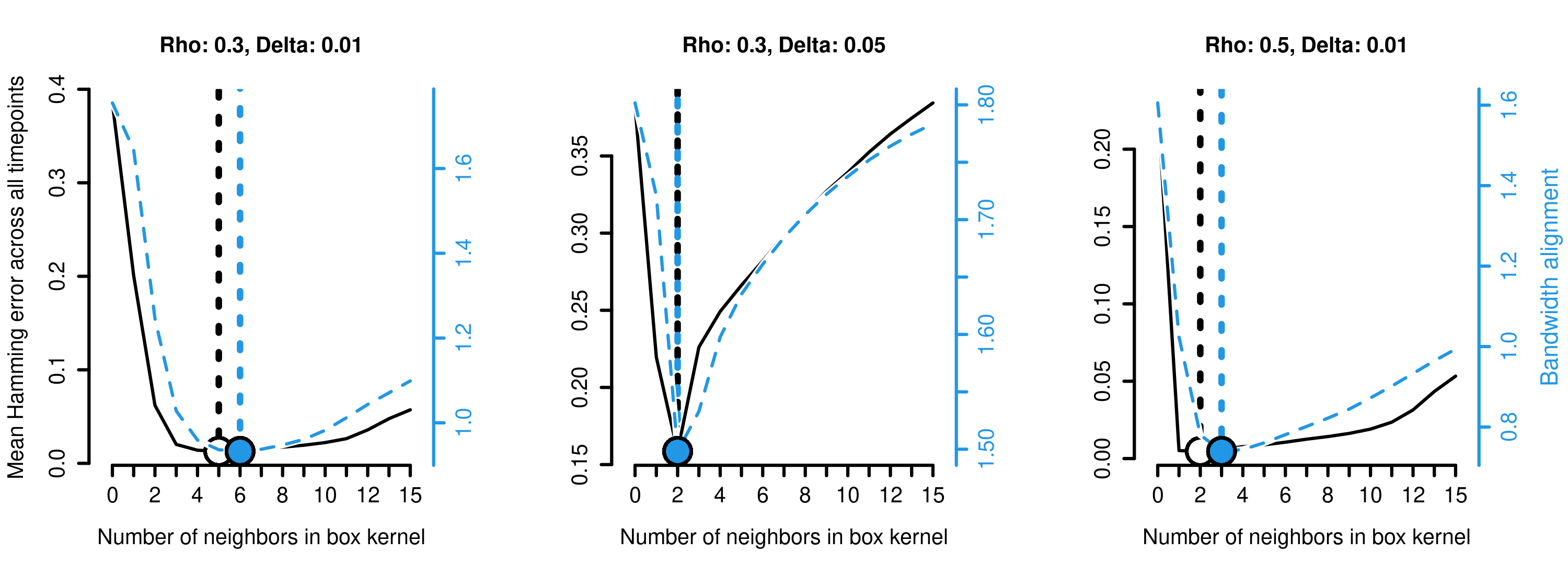
Figure figure: Simulation across three different settings of the community switching rate $\gamma$ and network density $\rho_{n}$ demonstrating KD-SoS’s performance for different bandwidth $r$’s. The Hamming error (equation) or the bandwidth score measured via $\sin\Theta$ (equation) are averaged across 25 trials for each $r$ (black and blue respectively), and the the vertical dotted lines denote the oracle minimizer of the Hamming error (black) and the chosen bandwidth $\widehat{r}$ using the tuning procedure (blue).

We first show our tuning procedure selects an appropriate bandwidth $r$ of the box kernel, as demonstrated in Figure figure. In the left panel, we fix $\rho_{n}=0.3$ and $\gamma=0.01$ and plot the mean Hamming error across all networks as a function of applying our estimator with the bandwidth $r$ (black line) and the bandwidth alignment used to tune $r$ (blue line), both averaged across 25 trials. A dot of their respective color marks the minimum of both curves. We make two observations. First, the Hamming error follows a classical U-shape as a function of $r$. This demonstrates that although a single network does not contain information to accurately estimate the communities (i.e., $r=0$), pooling information across too many networks is not ideal either since the community structures vary too much among the networks (i.e., $r=15$). Second, while a bandwidth of $r=5$ achieves the minimum Hamming error, our tuning procedure would select $r=6$ on average, and the degradation of the Hamming error is not substantial. We also vary $\rho_{n}$ and $\gamma$. When we set $\gamma$ to be 0.05 instead of $0.1$, we see that minimizing bandwidth becomes smaller, reflecting that fewer neighboring networks are relevant for estimating a particular network’s community structure. Alternatively, when we set $\rho_{n}$ to be 0.5 instead of 0.3, we see that minimizing bandwidth becomes smaller. However, as implied by the mean Hamming error on the y-axis, this is because more information is contained within each denser network, lessening the need to pool information across networks.

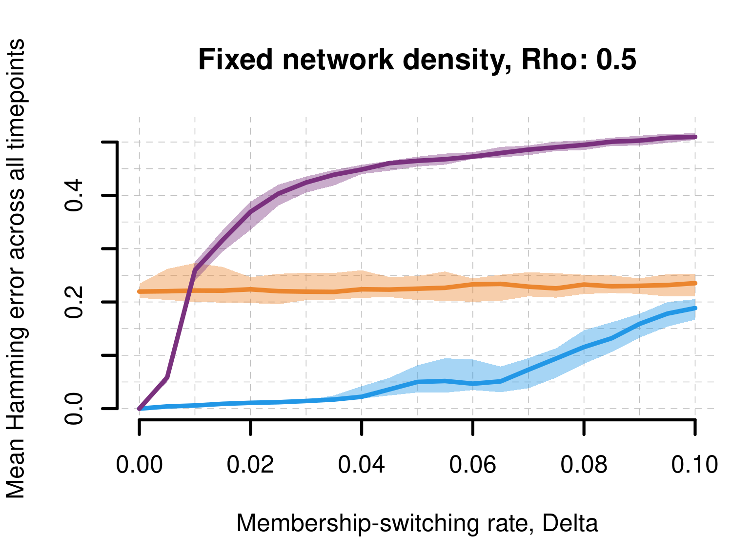
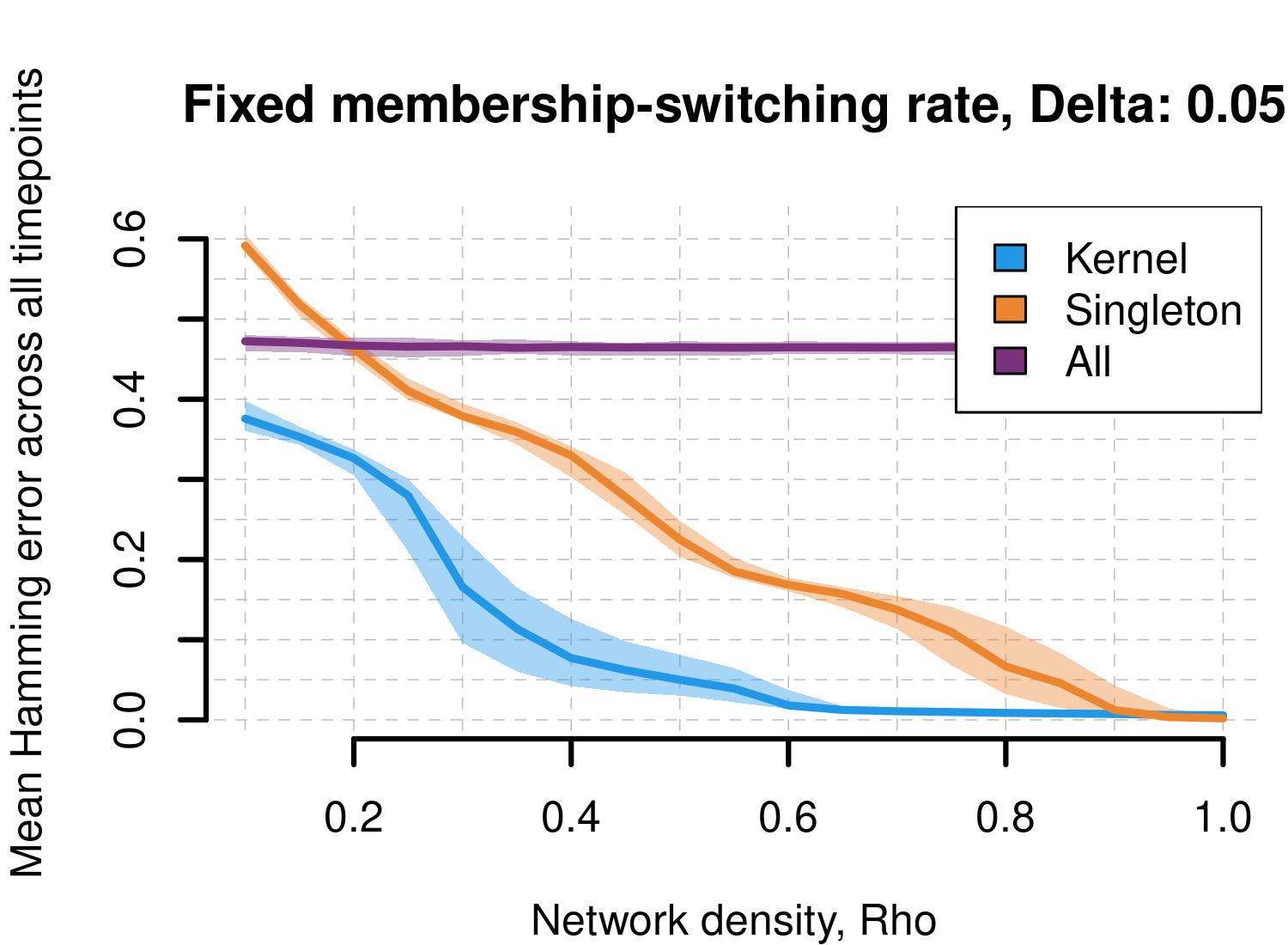
Figure figure: Simulation suite across three different settings of the community switching rate $\gamma$ and network density $\rho_{n}$ demonstrating KD-SoS with the bandwidth tuning procedure’s performance (“Kernel,” blue) compared to applying spectral clusterings to only one network at a time (“Singleton,” orange) or aggregating across all networks, akin to Lei & Lin (2022) (“All,” purple).

We now compare our method against other methods designed to estimate communities for the model (equation). Two natural candidates are our debiasing-and-smoothing method where the bandwidth is set to be $r=0$ (i.e., “Singleton,” where each network’s community is estimated using only that network) and $r=1$ (i.e., “All,” where each network’s community is estimated by equally weighting all the networks). We measure the performance of each of the three methods by computing the relative Hamming distance between $\widehat{M}^{(t)}$ and $M^{(t)}$, averaged across all time $t\in\mathcal{T}$ (i.e., a smaller metric implies better performance). Our results are shown in Figure figure. In the first simulation suite, we hold network density $\rho_{n}=0.5$ but vary the community switching rate $\gamma$ from $0$ to $0.1$ (i.e., stable communities to rapidly changing communities). Across the 50 trials for each value of $\gamma$, we see that KD-SoS (blue) can retain a small Hamming error below 0.2 across a wide range of $\gamma$. In contrast, observe that “Singleton” (orange) has a relatively stable performance, which is intuitive as the time-varying structure does not affect this method. Meanwhile, “All” (purple) degrades in performance quite rapidly as $\gamma$ increases due to aggregating among all the networks despite large differences in community structure. In the second simulation suite, we hold community switching rate $\gamma=0.05$ but vary the network density $\rho_{n}$ from $0.2$ to $1$ (i.e., sparse networks to dense networks). Across the 50 trials for each value of $\rho_{n}$, we see that KD-SoS (blue) performs better as $\rho_{n}$ increases, which is uniformly better than the “Singleton” (orange). This is sensible, as KD-SoS aggregates information across networks with an appropriately chosen bandwidth $r$. Meanwhile, “All” (purple) does not change in performance as $\rho_{n}$ increases because the time-varying community structure obstructs good performance regardless of network sparsity.

section.subsection Application to gene co-expression networks along developmental trajectories

We now return to the analysis of the developing brain introduced in Section section. We first enumerate descriptive summary statistics of these twelve networks, each of the same 993 genes. The median of the median degree across all twelve networks is 30.5 (range of 1 to 86, increasing with time), while the mean of the mean degree across all twelve networks is 52.8 (range of 4.6 to 121.9, also increasing with time). The median overall network sparsity, defined as the number of observed edges divided by the number of total possible edges, across all twelve networks is 5% (range of 0.4% to 12%, increasing with time). Lastly, if each network is analyzed separately, the median number of connected components is 97.5 (range of 34 to 452). However, if all the edges across all twelve networks are aggregated, there are two connected components (one with 981 genes, another with 12 genes).

We now describe the results when applying KD-SoS to the dataset. Due to the presence of only twelve networks with very different degrees, we use a Gaussian kernel normalized by each network’s leading singular value, i.e.,

$$Z^{(t;r)}=\sum_{s\in\mathcal{T}}\frac{w(s,t;r)}{\|A^{(s)}\|_{\operatorname{{op}}}}\cdot\Big{[}(A^{(s)})^{2}-D^{(s)}\Big{]},\quad\text{where }w(s,t;r)=\exp\Big{(}\frac{-(t-s)^{2}}{r^{2}}\Big{)}$$

instead of the aggregation used in (equation). While our theoretical developments in Theorem section.theorem do not use this estimator, our techniques would apply similarly to such estimators. Based on a scree plot among $\{A^{(t)}\}$, we chose $K=10$ as the dimensionality and number of communities. The bandwidth is chosen using our procedure in Section section.subsection, among the range of bandwidths $r$ that yielded alignable membership matrices as defined by Definition section.theorem. The membership results for three of the twelve networks are shown in Figure figure, where nodes of different colors are in different communities. Already, we can see gradual shifts in communities within these three networks. For example, both the purple and red communities grow in size as time progresses. Meanwhile, genes starting in the olive community eventually become part of the pink or white community.

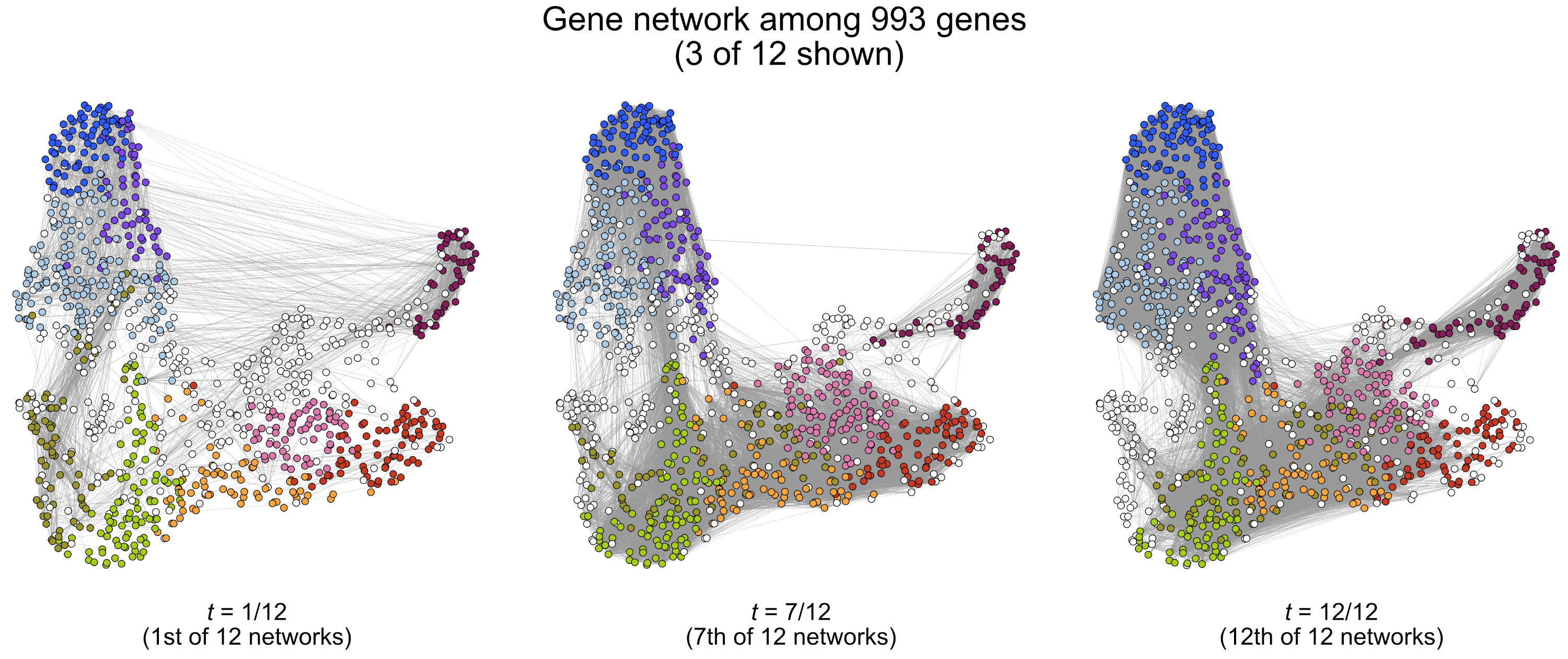
Figure figure: Three networks, as displayed in Figure figure, but with genes colored by the $K=10$ different communities via $K$ different colors as estimated by KD-SoS and the bandwidth tuning procedure.

It is hard to discern the broad summary of how communities are related across time from Figure figure. Hence, we plot the percentage of genes that exit from one community to join a different community between the first three networks in Figure figure. Our tuning bandwidth procedure chooses an $r$ that yields relatively stable communities across time. Meanwhile, Figure figure also visualizes the latent 10-dimensional embedding among all 993 genes for the first three networks. We observe that: 1) the SBM model is appropriate for modeling the dataset at hand since the heatmaps demonstrate strong block structure, and 2) a choice of $K=10$ seems visually appropriate, as none of the 10 communities seem to represent sub-communities based on the 10 latent dimensions.

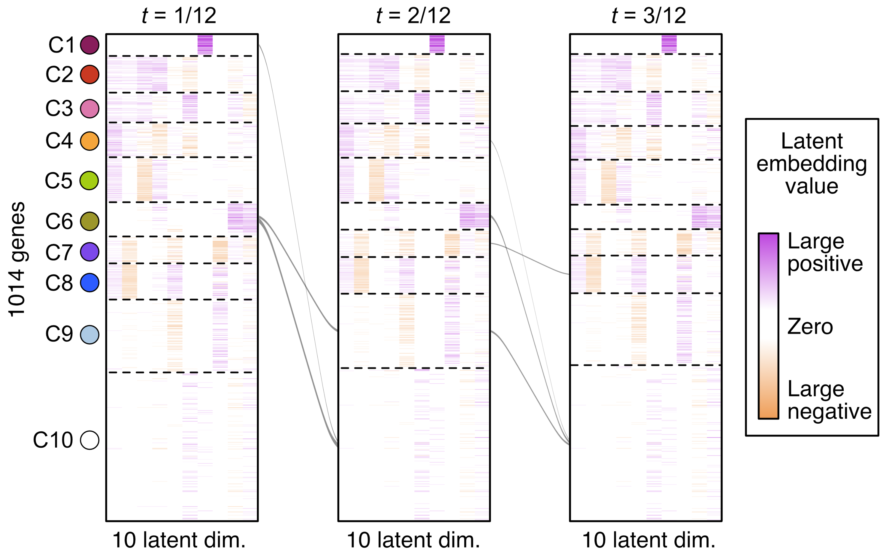
Figure figure: The heatmap of the first three network’s leading $K=10$ eigenvectors, where the 993 genes are ordered based on their assigned communities, with their colors (left) corresponding to those in Figure figure. Let $s,t\in[0,1]$ denote two consecutive two times where $s<t$. The size of the arrow connecting two different communities, one at $s$ and another at $t$, denotes the percentage of genes that leave the community at time $s$ to a different community at time $t$, ranging from 1% of the genes in the community (thin arrow) to 10% (thick arrow).

Now that we have investigated the appropriateness of the time-varying SBM model, we now address the motivating biological questions asked in Section section – what new insights about the glutamatergic development that we could investigate based on the dynamic network structure that we couldn’t have inferred based on only analyzing the mean? We focus specifically on the fifth and twelfth networks here. Starting with the fifth network (Figure figureA), we show the enriched gene ontology (GO) terms for the selected communities in Table section.subsection to inquire about the functionality of each set of genes. For example, community 2 (red) is highly enriched for coordinated genes related to neurogenesis despite these genes not yet having high mean expression. In contrast, community 6 (olive) contains genes related to nervous system development with high gene expression but are not as coordinated. Meanwhile, community 8 (blue) is highly enriched for coordinated and highly expressed genes related to cellular component biogenesis. Likewise, in the twelfth network (Figure figureA and Table section.subsection), community 1 (burgundy) is highly enriched for coordinated genes related to cell cycle, despite these genes not yet having high mean expression. In contrast, community 2 (red) is still highly enriched for genes related to neurogenesis (the same as the fifth network), but now these genes are highly expressed but not coordinated. Lastly, community 7 (purple) is highly enriched for coordinated and highly expressed genes related to the metabolic process. Altogether, these results demonstrate that investigating the dynamics of gene coordination can give an alternative perspective on brain development.

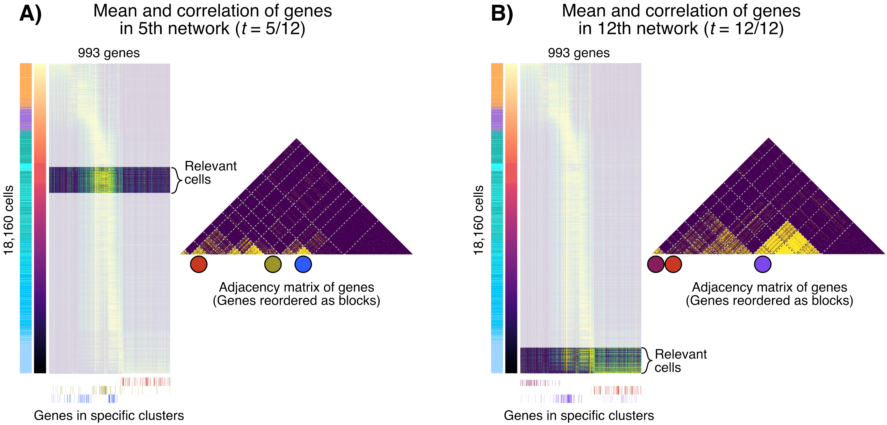
Figure figure: Correlation networks for the second (A) or twelfth (B) timepoints, where the cells corresponding to the respective bin of pseudotimes are highlighted via the cell-gene heatmap (left) and the corresponding adjacency matrix among 993 genes where the genes are organized based on their estimated memberships for the respective timepoint (right). The cell-gene heatmaps are the same as in Figure figure. Below the heatmaps marks the genes (i.e., columns) that are part of specifically highlighted communities, corresponding to the marked entries of the adjacency matrices.

Description of select gene communities for network $t=5/12$ Summary stat. Gene set enrichment # genes Mean value (std.) Connectivity GO term % of community FDR p-value Community 2 (Red) 76 0.06 (0.08) 0.72 GO:0022008 (Neurogenesis) 29% $2.91\times 10^{-6}$ Community 6 (Olive) 65 0.51 (0.36) 0.23 GO:0007399 (Nervous system development) 32% $7.66\times 10^{-3}$ Community 8 (Blue) 74 0.54 (0.27) 0.88 GO:0044085 (Cellular component biogenesis) 36% $2.74\times 10^{-4}$ Select gene communities for network $t=5/12$, depicting (from left to right) the number of genes in the community, the mean gene expression value and standard deviation among all the cells in this partition (after each gene is standardized across all 18,160 cells), the percent of edges among the genes in the community, an enriched GO term among these genes, the percentage of genes in this community that are in this GO term, and the GO term’s FDR value.

Description of select gene communities for network $t=12/12$ Summary stat. Gene set enrichment # genes Mean value (std.) Connectivity GO term % of community FDR p-value Community 1 (burgundy) 57 0.01 (0.03) 0.66 GO:0007049 (Cell cycle) 68% $4.42\times 10^{-32}$ Community 2 (Red) 71 0.52 (0.32) 0.13 GO:0022008 (Neurogenesis) 24% $1.43\times 10^{-3}$ Community 7 (Purple) 89 0.43 (0.35) 0.77 GO: 0008152 (Metabolic process) 63% $9.57\times 10^{-3}$ Select gene communities for network $t=12/12$, displayed in the same layout as Table 1.

Additional plots corresponding to networks not shown in Figures figure through figure as well as additional visualizations of the time-varying dynamics are included in the Appendix.

section Discussion

We establish a bridge between time-varying network analysis and non-parametric analysis in this paper, demonstrating that smoothness across the connectivity matrices $\{B^{(t)}\}$ is not required for consistent community detection. We achieve this through a novel bias-variance decomposition, whereby we project networks close to time $t$ onto the leading eigenspace of the network at time $t$. While our paper has demonstrated how to relate the discrete changes in nodes’ communities to the typically continuous non-parametric theory, there are two major theoretical directions we hope our work can aid for future research. The first is refining this relation between time-varying networks and non-parametric analyses. While previous work for time-varying networks such as Pensky & Zhang (2019) and Keriven & Vaiter (2022) derived rates reliant on the smoothness across $\{B^{(t)}\}$, it is unclear from a minimax perspective how the community estimation rates improve as $\{B^{(t)}\}$ evolve according to a smoother process. Additionally, there have been major historical developments in non-parametric analysis through local polynomials and trend filtering. These address the so-called boundary bias typical in non-parametric regression and construct estimators that inherently adapt to the data’s smoothness. We wonder if there are analogies for these estimators for the time-varying SBM setting. Secondly, as with any non-parametric estimator, there are unanswered questions about how to best tune estimators such as KD-SoS. As we described in Section section.subsection, tuning procedures reliant on prediction, such as cross-validation, are unlikely to be fruitful for the setting we study. However, recent ideas using leave-one-out analysis or sharp $\ell_{2\rightarrow\infty}$ estimation bounds for the leading eigenspaces have successfully derived cross-validation-like approaches in other network settings. We believe those ideas can be used similarly in our setting where $\{B^{(t)}\}$ is not assumed to be positive definite or smoothly varying.

Data and code reproducibility

The human brain development dataset (Trevino et al., 2021) was downloaded from https://www.ncbi.nlm.nih.gov/geo/query/acc.cgi?acc=GSE162170, specifically the GSE162170_rna_counts.tsv.gz and GSE162170_rna_cell_metadata.txt files. (Alternatively, the data can also be accessed via https://github.com/GreenleafLab/brainchromatin.) We use the author’s clustering information derived from the Supplementary Information of Trevino et al. (2021), Table S1 (file: 1-s2.0-S0092867421009429-mmc1.xlsx, Sheet F), and genes from Table S1 and Table S3 (files: 1-s2.0-S0092867421009429-mmc1.xlsx, Sheet G and 1-s2.0-S0092867421009429-mmc3.xlsx, Sheet A). The code for the KD-SoS as well as all simulations and analyses (including the details on how we preprocessed the single-cell RNA-seq data) is in https://github.com/linnykos/dynamicGraphRoot.

Supplementary material

In the supplementary materials, we include the proofs of Lemma section.theorem, Theorem section.theorem, Corollary section.theorem, Corollary section.theorem, Corollary section.theorem, Proposition section.theorem, Proposition section.theorem, and Proposition section.theorem. We also include preprocessing details and more supplemental results in the scRNA-seq analysis from Section section.subsection.

Proofs

Proof for bias-variance tradeoff

Proof of Lemma section.theorem.

Proof .theorem.

The proof is straightforward after observing for any $t\in\mathcal{T}$,

$$(A^{(t)})^{2}=(P^{(t)}+X^{(t)})^{2}=(P^{(t)})^{2}+P^{(t)}X^{(t)}+X^{(t)}P^{(t)}+(X^{(t)})^{2}.$$

and furthermore,

$$(P^{(t)})^{2}=(Q^{(t)})^{2}+\big{[}\operatorname{{diag}}(Q^{(t)})\big{]}^{2}-Q^{(t)}\operatorname{{diag}}(Q^{(t)})-\operatorname{{diag}}(Q^{(t)})Q^{(t)}.$$

Proof of Theorem section.theorem.

Proof .theorem.

Let $c$ be a constant that can vary from term to term, depending only on the constants $c_{1}$, $c_{2}$, $c_{3}$, $c_{\delta}$, and $K$. Consider the decomposition in Lemma section.theorem, where we focus on the time $t\in\mathcal{T}$. We start with the membership bias term (i.e., term $I$). Let $\|\cdot\|_{\operatorname{{op}}}$ denote the operator norm (i.e., largest singular value). For $h=c\cdot(\gamma r+\log(n)/n)$ for a bandwidth of length $r$, consider the event that

$$\mathcal{E} =\underbrace{\Big{\{}\max_{s\in\mathcal{S}(t;r)}L\big{(}M^{(s)},M^{(t)}\big{)}\leq h\Big{\}}}_{\mathcal{E}_{1}}\bigcap\underbrace{\Big{\{}n_{k}^{(t)}\in\Big{[}\frac{1}{cK}\cdot n,\frac{c}{K}\cdot n\Big{]},\quad\text{for all }k\in\{1,\ldots,K\},\;t\in\mathcal{T}\Big{\}}}_{\mathcal{E}_{2}}.$$ (equation)

Lemma .theorem shows that the event $\mathcal{E}_{1}$ happens with probability at least $1-1/n$, and the event $\mathcal{E}_{2}$ is controlled by Assumption section.subsection. Hence, by union bound, this means event $\mathcal{E}$ happens with probability at least $1-1/n-\epsilon_{c_{2},n}$.

The remainder of our analysis will be done in the intersection with event $\mathcal{E}$. We start by analyzing the minimum eigenvalue of the target term (i.e., term $V$ in (equation)). We define $\widetilde{M}^{(t)}=M^{(t)}\big{(}\Delta^{(t)}\big{)}^{-1/2}$ as well as

$$\widetilde{B}^{(t)}=\big{(}\Delta^{(t)}\big{)}^{1/2}B^{(t)}\big{(}\Delta^{(t)}\big{)}^{1/2},$$ (equation)

so that $Q^{(t)}=\rho_{n}\cdot M^{(t)}B^{(t)}(M^{(t)})^{\top}=\rho_{n}\cdot\widetilde{M}^{(t)}\widetilde{B}^{(t)}(\widetilde{M}^{(t)})^{\top}$. Also recall that the definition of the projection matrix $\Pi^{(t)}=\widetilde{M}^{(t)}(\widetilde{M})^{\top}$. We start with the observation that

$$\Big{\|}\sum_{s\in\mathcal{S}(t;r)}\Pi^{(t)}(Q^{(s)})^{2}\Pi^{(t)}\Big{\|}_{\operatorname{{op}}}=\Big{\|}\sum_{s\in\mathcal{S}(t;r)}\widetilde{M}^{(t)}(\widetilde{M}^{(t)})^{\top}(Q^{(s)})^{2}\widetilde{M}^{(t)}(\widetilde{M}^{(t)})^{\top}\Big{\|}_{\operatorname{{op}}}$$

$$=\rho_{n}^{2}\cdot\Big{\|}\sum_{s\in\mathcal{S}(t;r)}\underbrace{(\widetilde{M}^{(t)})^{\top}\widetilde{M}^{(s)}}_{=U^{(t;s)}}(\widetilde{B}^{(s)})^{2}(\widetilde{M}^{(s)})^{\top}\widetilde{M}^{(t)}\Big{\|}_{\operatorname{{op}}}$$

$$\overset{(i)}{\geq}\rho_{n}^{2}\cdot\Big{\|}\sum_{s\in\mathcal{S}(t;r)}\sigma_{\min}^{2}(U^{(t;s)})\cdot(\widetilde{B}^{(s)})^{2}\Big{\|}_{\operatorname{{op}}}\geq\rho_{n}^{2}\cdot\Big{\|}\Big{[}\min_{s\in\mathcal{S}(t;r)}\Big{\{}\sigma^{2}_{\min}\big{(}U^{(t;s)}\big{)}\Big{\}}\Big{]}\sum_{s\in\mathcal{S}(t;r)}(\widetilde{B}^{(s)})^{2}\Big{\|}_{\operatorname{{op}}}$$

$$\overset{(ii)}{\geq}(1-ch^{1/2})\cdot\rho_{n}^{2}\cdot\Big{\|}\sum_{s\in\mathcal{S}(t;r)}(\widetilde{B}^{(s)})^{2}\Big{\|}_{\operatorname{{op}}}\overset{(iii)}{\geq}c\cdot(1-ch^{1/2})\cdot\widetilde{T}\rho_{n}^{2}n^{2},$$ (equation)

where $\widetilde{T}=|\mathcal{S}(t;r)|=\min\{2rT+1,T\}$ denotes the number of networks with non-zero weights via the box kernel of bandwidth $r$. Here, $(i)$ holds by the variational characterization of eigenvalues (i.e., Rayleigh-Ritz theorem), $(ii)$ holds using Lemma .theorem, the definition of $h$ under the event $\mathcal{E}$ in (equation), as well as $(1-x)^{2}=1-2x+x^{2}\geq 1-2x$ for $x<1$, and $(iii)$ holds via Assumptions section.subsection and section.subsection and the definition of $\widetilde{B}$ in (equation).

We now move to upper-bound relevant terms in (equation). Recall that $\sigma_{\min}(A)$ denote the smallest singular value of a matrix $A$. For term $I$, observe that

$$\Big{\|}(Q^{(s)})^{2}-\Pi^{(t)}(Q^{(s)})^{2}\Pi^{(t)}\Big{\|}_{\operatorname{{op}}}=\Big{\|}\Pi^{(s)}(Q^{(s)})^{2}\Pi^{(s)}-\Pi^{(t)}(Q^{(s)})^{2}\Pi^{(t)}\Big{\|}_{\operatorname{{op}}}$$

$$\overset{(i)}{\leq}\underbrace{\Big{(}\Big{\|}\widetilde{M}^{(s)}(\widetilde{M}^{(s)})^{\top}\Big{\|}_{\operatorname{{op}}}+\Big{\|}\widetilde{M}^{(t)}(\widetilde{M}^{(t)})^{\top}\Big{\|}_{\operatorname{{op}}}\Big{)}}_{=2}\Big{\|}(Q^{(s)})^{2}\Big{\|}_{\operatorname{{op}}}\Big{\|}\widetilde{M}^{(s)}(\widetilde{M}^{(s)})^{\top}-\widetilde{M}^{(t)}(\widetilde{M}^{(t)})^{\top}\Big{\|}_{\operatorname{{op}}}$$

$$\overset{(ii)}{\leq}c\rho_{n}^{2}n^{2}h^{1/2}$$ (equation)

where in $(i)$, we used $ADA^{\top}-BDB^{\top}=ADA^{\top}\pm ADB^{\top}-BDB^{\top}=AD(A-B)^{\top}+(A-B)DB^{\top}$, and $(ii)$ holds using Lemma .theorem and Lemma .theorem for some constant $c$ that depends polynomially on $c_{2}$ and $K$ (recalling the asymptotics in Assumption section.subsection).

For the remaining terms (i.e., terms $II$, $III$ and $IV$), since we are considering the regime where $\widetilde{T}^{1/2}n\rho_{n}\geq c_{3}\log^{1/2}(\widetilde{T}+n)$, we invoke the techniques in Theorem 1 of Lei & Lin (2022),

$$\Big{\|}\sum_{s\in\mathcal{S}(t;r)}\big{[}\operatorname{{diag}}(Q^{(t)})\big{]}^{2}-Q^{(t)}\operatorname{{diag}}(Q^{(t)})-\operatorname{{diag}}(Q^{(t)})Q^{(t)}\Big{\|}_{\operatorname{{op}}}\leq\widetilde{T}n\rho_{n}^{2},$$ (equation)

$$\Big{\|}\sum_{s\in\mathcal{S}(t;r)}X^{(s)}P^{(s)}+P^{(s)}X^{(s)}\Big{\|}_{\operatorname{{op}}}\leq c\cdot\widetilde{T}^{1/2}n^{3/2}\rho_{n}^{3/2}\log^{1/2}(\widetilde{T}+n),$$ (equation)

$$\Big{\|}\sum_{s\in\mathcal{S}(t;r)}(X^{(s)})^{2}-D^{(s)}\Big{\|}_{\operatorname{{op}}}\leq\widetilde{T}n\rho_{n}^{2}+c\cdot\widetilde{T}^{1/2}n\rho_{n}\log^{1/2}(\widetilde{T}+n),$$ (equation)

the second and third which hold with probability at least $1-O((\widetilde{T}+n)^{-1})$.

Consider the eigen-decomposition,

$$\Big{[}\sum_{s\in\mathcal{S}(t;r)}\Pi^{(t)}(Q^{(s)})^{2}\Pi^{(t)}\Big{]}=U^{(t;r)}\Lambda^{(t;r)}\big{(}U^{(t;r)}\big{)}^{\top},$$

and observe that the eigen-basis of $Q^{(t)}$ is also $U^{(t;r)}$ (i.e., there is a $K\times K$ orthonormal matrix $\Theta$ such that the eigen-basis of $Q^{(t)}$ is equal to $U^{(t;r)}\Theta$, see Lemma 2.1 of Lei & Rinaldo (2015). Recall that $\widehat{U}^{(t;r)}$ is the eigen-basis estimated by KD-SoS. Putting everything together and recalling that the product of two orthonormal matrices yields an orthonormal matrix, we see that with an application of Davis-Kahan (see Theorem 2 of Yu et al. (2014)), there exists a unitary matrix $\widehat{O}\in\mathbb{R}^{K\times K}$ such that

$$\big{\|}\widehat{U}^{(t;r)}\widehat{O}-U^{(t;r)}\big{\|}_{F}\leq\frac{2^{3/2}K^{1/2}\big{\|}\big{[}\sum_{s\in\mathcal{S}(t;r)}(A^{(s)})^{2}-D^{(s)}\big{]}-\big{[}\sum_{s\in\mathcal{S}(t;r)}\Pi^{(t)}(Q^{(s)})^{2}\Pi^{(t)}\big{]}\big{\|}_{\operatorname{{op}}}}{\lambda_{\min}\big{(}\sum_{s\in\mathcal{S}(t;r)}\Pi^{(t)}(Q^{(s)})^{2}\Pi^{(t)}\big{)}}$$

$$\overset{(i)}{\leq}c\cdot\frac{h^{1/2}\widetilde{T}n^{2}\rho_{n}^{2}+\widetilde{T}n\rho_{n}^{2}+\widetilde{T}^{1/2}n^{3/2}\rho_{n}^{3/2}\log^{1/2}(\widetilde{T}+n)+\widetilde{T}n\rho_{n}^{2}+\widetilde{T}^{1/2}n\rho_{n}\log^{1/2}(\widetilde{T}+n)}{(1-ch^{1/2})_{+}\cdot\widetilde{T}n^{2}\rho_{n}^{2}}$$

$$\overset{(ii)}{\leq}\frac{ch^{1/2}}{(1-ch^{1/2})_{+}}+\frac{2c}{(1-ch^{1/2})_{+}\cdot n}+\frac{c\log^{1/2}(\widetilde{T}+n)}{(1-ch^{1/2})_{+}\cdot\widetilde{T}^{1/2}n\rho_{n}},$$

where $(i)$ holds with an application of Lemma section.theorem as well as Equations (equation), (equation), (equation), and (equation), and $(ii)$ holds since $n\rho_{n}\leq c_{1}$ (due to Assumption section.subsection).

Lastly, we wish to convert a Frobenius norm bound between the true and estimated orthonormal matrices into a misclustering error rate. To do this, from Lemma 2.1 of Lei & Rinaldo (2015), we know the minimum Euclidean distance between distinct rows of $U^{(t;r)}$ is at least $c/\sqrt{n}$. Hence, by invoking Lemma D.1 of Lei & Lin (2022) (i.e., a simplification of Lemma 5.3 of Lei & Rinaldo (2015)), the number of misclustered nodes by spectral clustering is no larger than

$$c\cdot\Big{(}\frac{hn}{(1-ch^{1/2})_{+}^{2}}+\frac{1}{(1-ch^{1/2})_{+}^{2}\cdot n}+\frac{\log(\widetilde{T}+n)}{(1-ch^{1/2})_{+}^{2}\cdot\widetilde{T}n\rho_{n}^{2}}\Big{)}.$$

We divide the above term by $n$ to obtain the percentage of misclustered nodes.

Proof for Corollary section.theorem.

Proof .theorem.

Let $c$ be a constant that can vary from term to term, depending only on the constants $c_{1}$, $c_{2}$, $c_{3}$, $c_{\delta}$, and $K$. We seek to derive a the near-optimal bandwidth $r^{*}$. Consider the rate in Theorem section.theorem. We will only consider the regime where

$$\gamma r\ll 1,$$

which would mean the leading term in the rate in Theorem section.theorem is upper-bounded by a constant, i.e.,

$$\frac{1}{(1-(\gamma r+\log(n)/n)^{1/2})^{2}_{+}}\ll c.$$

This allows us to ignore this leading term when deriving the functional form of $r^{*}$.

Next, observe that if we only want to derive the optimal bandwidth $r^{*}$ up to logarithmic factors, we can define

$$r^{*}=\min_{r\in[0,1]}\underbrace{c\cdot\gamma r}_{=A(r)}+\underbrace{\frac{\log(T+n)}{rTn^{2}\rho_{n}^{2}}}_{=B(r)}.$$

Setting the derivative of $A(r)+B(r)$ to be 0 yields,

$$0=c\cdot\gamma-\frac{1}{(r^{*})^{2}Tn^{2}\rho_{n}^{2}}\quad\Longrightarrow\quad r^{*}=c\cdot\frac{1}{(\gamma T)^{1/2}n\rho_{n}},$$

for some constant $c$ that depends on $c_{1}$, $c_{2}$, $c_{3}$, $c_{\delta}$, and $K$.

Proof for Corollary section.theorem and Corollary section.theorem.

Proof .theorem.

The upper-bound of the relative Hamming distance depends on if $r^{*}\rightarrow 1$ or $r^{*}\rightarrow 0$ based on the asymptotic sequence of $n$, $T$, $\gamma$ and $\rho_{n}$. Recall that by assumptions in Theorem section.theorem, we require

$$(rT+1)^{1/2}n\rho_{n}=\omega\Big{(}\log^{1/2}(rT+n+1)\Big{)}.$$ (equation)

• Based on Corollary section.theorem, the scenario $r^{*}\rightarrow 1$ occurs if

  $$\frac{1}{(\gamma T)^{1/2}n\rho_{n}}\rightarrow\infty\quad\iff\quad(\gamma T)^{1/2}n\rho_{n}\rightarrow 0.$$

  We also require that $\gamma r^{*}\rightarrow 0$ as a necessary condition for the relative Hamming distance in Theorem section.theorem to converge to 0. To ensure this, we will require asymptotically

  $$\gamma\rightarrow 0.$$ (equation)

  Furthremore, the requirement (equation) is satisfied if

  $$T^{1/2}n\rho_{n}=\omega\big{(}\log^{1/2}(T+n)\big{)}.$$ (equation)

  To upper-bound the relative Hamming error, since $\gamma r^{*}\rightarrow 0$, for any constant $c$, this means somewhere along this asymptotic sequence of $\{n,T,\gamma,\rho_{n}\}$, we are guaranteed $\gamma r+\log(n)/n\leq c$ for the remainder of the asymptotic sequence. Then,

  $$L\big{(}G^{(t)},\widehat{G}^{(t)}\big{)}=O\Big{(}\gamma+\frac{\log(n)}{n}+\frac{1}{n^{2}}+\frac{\log(T+n)}{Tn^{2}\rho^{2}_{n}}\Big{)},$$

  By (equation) and (equation), we are ensured that $L\big{(}G^{(t)},\widehat{G}^{(t)}\big{)}$ converges to 0.

• Based on Corollary section.theorem, the scenario $r^{*}\rightarrow 0$ occurs if

  $$\frac{1}{(\gamma T)^{1/2}n\rho_{n}}\rightarrow 0\quad\iff\quad(\gamma T)^{1/2}n\rho_{n}\rightarrow\infty.$$ (equation)

  We also require that $\gamma r^{*}\rightarrow 0$ as a necessary condition for the relative Hamming distance in Theorem section.theorem to converge to 0. To ensure this, using the rate of $r^{*}$ derived in Corollary section.theorem, we require asymptotically

  $$\quad\gamma r^{*}=\frac{\gamma^{1/2}}{T^{1/2}n\rho_{n}}\rightarrow 0\quad\iff\quad\gamma=o\big{(}T(n\rho_{n})^{2}\big{)},$$ (equation)

  which upper-bounds the maximum $\gamma$ before KD-SoS is no longer consistent. Furthermore, the requirement (equation) is satisfied based on the bandwidth $r^{*}$ in Corollary section.theorem if

  $$\Big{(}\frac{T}{\gamma}\Big{)}^{1/2}n\rho_{n}=\omega\big{(}\log^{1/2}(T+n)\big{)}.$$ (equation)

  An asymptotic regime that would satisfy (equation), (equation), and (equation) is

  $$\gamma\text{ is increasing and }\gamma=o\Big{(}\frac{T(n\rho_{n})^{2}}{\log(T+n)}\Big{)}.$$ (equation)

  To upper-bound the relative Hamming error, since $\gamma r^{*}\rightarrow 0$, for any constant $c$, this means somewhere along this asymptotic sequence of $\{n,T,\gamma,\rho_{n}\}$, we are guaranteed $\gamma r+\log(n)/n\leq c$ for the remainder of the asymptotic sequence. Then,

  $$L\big{(}G^{(t)},\widehat{G}^{(t)}\big{)}=O\Big{(}\frac{\gamma^{1/2}}{T^{1/2}n\rho_{n}}+\frac{\log(n)}{n}+\frac{1}{n^{2}}+\frac{\gamma^{1/2}\log(T^{1/2}/(\gamma^{1/2}n\rho_{n})+n)}{T^{1/2}n\rho_{n}}\Big{)}.$$

  By (equation), we are ensured that $L\big{(}G^{(t)},\widehat{G}^{(t)}\big{)}$ converges to 0.

Hence, we are done.

Proof of Proposition section.theorem.

Proof .theorem.

We split the proof into two parts.

Deterministic component. Here, we prove if more than $n/2$ nodes change memberships between $M^{(t)}$ and $M^{(t+1/T)}$ for a particular $t\in\mathcal{T}\backslash\{1\}$, then $M^{(t)}$ and $M^{(t+1/T)}$ are not alignable. Then, by definition, the entire sequence of memberships is not alignable.

Consider the confusion matrix $C\in\{0,\ldots,n\}^{K\times K}$ formed from $M^{(t)}$ and $M^{(t+1/T)}$. Since more than $n/2$ nodes change memberships, then by definition, the sum of the off-diagonal entries in $C$ must be larger than $n/2$, and the sum of the diagonal entries in $C$ must be smaller than $n/2$. Hence, there must exist a diagonal entry in $C$ whereby it is smaller than its respective column-sum or row-sum. Hence, it must be the case that either $C$ or $C^{\top}$ is not diagonally dominant, and hence, $M^{(t)}$ and $M^{(t+1/T)}$ is not alignable.

Probabilistic component. Here, we prove that if $\gamma$ is large relative to $T$, then there is a non-vanishing probability that more than $n/2$ nodes change memberships between $M^{(t)}$ and $M^{(t+1/T)}$ for some time $t\in\mathcal{T}\backslash\{1\}$.

Towards this end, let $X^{(t)}$ denote the total number of instances when nodes change communities between time $t$ and $t+1/T$ based on Assumption section.subsection. (Note, this random variable is not a Poisson, since the Poisson process denotes the number of instances a node changes membership, not the number of unique nodes change membership.) We are interested in when the probability $X^{(t)}\geq n/2$ for some $t\in\{1/T,\ldots,(T-1)/T\}$ is bounded away from 0. That is,

$$\mathbb{P}\Big{(}X^{(t)}\geq n/2,\text{ for some }t\in\{1/T,\ldots,(T-1)/T\}\Big{)}$$

$$=1-\mathbb{P}\Big{(}X^{(t)}\leq n/2,\text{ for all }t\in\{1/T,\ldots,(T-1)/T\}\Big{)}$$

$$=1-\mathbb{P}\Big{(}X^{(1/T)}\leq n/2\Big{)}^{T-1}=1-\Big{[}1-\mathbb{P}\Big{(}X^{(1/T)}\geq n/2\Big{)}\Big{]}^{T-1}$$ (equation)

To lower-bound the RHS of (equation), consider a probability $p$ that a node changes membership in a time interval of length $1/T$. Since each node changes memberships independently of one another, the total number of nodes that change memberships is modeled as $X^{(1/T)}=\text{Binomial}(n,p)$ for a $p$ to be determined, and we are interested the probability that $X^{(1/T)}\geq n/2$. Certainly, if $p=1/2$, then the probability of $X^{(1/T)}\geq n/2$ is strictly bounded away from 0. Hence, we are interested in a $p$ less than $1/2$.

Towards this end, invoking a lower-bound of the upper-tail of a Binomial (see Chernoff-Hoeffding bounds in references such as Pelekis (2016)), observe that

$$\mathbb{P}\big{(}X^{(1/T)}\geq n/2\big{)}\geq\frac{1}{\sqrt{2n}}\exp\Big{(}-nD\big{(}\frac{1}{2}\;||\;p\big{)}\Big{)},$$ (equation)

where

$$D\big{(}\frac{1}{2}\;||\;p\big{)} =\frac{1}{2}\cdot\log\Big{(}\frac{1/2}{p}\Big{)}+\frac{1}{2}\cdot\log\Big{(}\frac{1/2}{1-p}\Big{)}$$

$$=\frac{-1}{2}\cdot\log\big{(}2\cdot p\big{)}+\frac{-1}{2}\cdot\log\big{(}2\cdot(1-p)\big{)}$$

$$=\log\Big{[}\big{(}4\cdot p\cdot(1-p)\big{)}^{-1/2}\Big{]}.$$ (equation)

For reasons we will shortly discuss, we are interested when (equation) is lower-bounded by $1/(T-1)$. Hence, combining (equation) with (equation), we are interested in $x$ such that

$$\mathbb{P}\big{(}X^{(0)}\geq n/2\big{)}\geq\frac{1}{\sqrt{2n}}\cdot\Big{(}\big{(}4\cdot p\cdot(1-p)\big{)}^{n/2}\Big{)}\geq\frac{1}{T-1},$$ (equation)

which is equivalent to

$$p\cdot(1-p)\geq\frac{1}{4}\cdot\Big{(}\frac{(2n)^{1/2}}{T-1}\Big{)}^{2/n}.$$ (equation)

Observe that if we assume that $p\leq 1/2$, then a value of $p$ that satisfies

$$p^{2}\geq\frac{1}{4}\cdot\Big{(}\frac{(2n)^{1/2}}{T-1}\Big{)}^{2/n}\quad\iff\quad p\geq\frac{1}{2}\cdot\Big{(}\frac{(2n)^{1/2}}{T-1}\Big{)}^{1/n}$$ (equation)

is ensured to satisfy (equation).

This means if $1/2\cdot((2n)^{1/2}/(T-1))^{1/n}\leq p\leq 1/2$, then there is at least probability $1/(T-1)$ that $X^{(1/T)}\geq n/2$. Therefore, using this value of $p$, we infer from (equation) that

$$\Big{[}1-\mathbb{P}\Big{(}X^{(1/T)}\geq n/2\Big{)}\Big{]}^{T-1}\leq\big{(}1-\frac{1}{T-1}\big{)}^{T-1}\overset{(i)}{\leq}1/e\approx 0.37,$$ (equation)

where $(i)$ uses $\lim_{x\rightarrow\infty}(1-1/x)^{x}=1/e$ from below. Plugging (equation) back into (equation) shows for probability $p$ that a node changes membership within any time interval of length $1/T$, then for any $T\geq 2$,

$$\mathbb{P}\Big{(}X^{(t)}\geq n/2,\text{ for some }t\in\{1/T,\ldots,(T-1)/T\}\Big{)}\geq 1-1/e\approx 0.63.$$

Lastly, we are now interested in the relation between $\gamma$ and $T$ such that there is at least a probability $p$ of a node changing memberships in a time interval of length $1/T$. By the Poisson process in Assumption section.subsection, the probability a node changes membership in such an interval is

$$1-\exp(-\gamma/T) \geq p=\frac{1}{2}\cdot\Big{(}\frac{(2n)^{1/2}}{T-1}\Big{)}^{1/n}$$

$$\Longrightarrow\quad\gamma \geq T\cdot\log\bigg{[}\bigg{(}1-\frac{1}{2}\cdot\Big{(}\frac{(2n)^{1/2}}{T-1}\Big{)}^{1/n}\bigg{)}^{-1}\bigg{]}$$

Hence, we are done.

Proof of Proposition section.theorem.

Proof .theorem.

Consider a particular time $t\in\mathcal{T}\backslash\{1\}$. For any time $t$ and $t+1/T$, consider the confusion matrix $C^{(t,t+1/T)}$ formed between membership matrices $M^{(t)}$ and $M^{(t+1/T)}$. Let $C=C^{(t,t+1/T)}$ for notational simplicity. Let $m_{\min}$ denote the size of the smallest community at time $t$,

$$m_{\min}=\min_{k\in\{1,\ldots,K\}}\sum_{i=1}^{n}M_{ik}^{(t)}=\min_{k\in\{1,\ldots,K\}}\sum_{\ell=1}^{K}C_{k\ell}.$$

Consider any community $k\in\{1,\ldots,K\}$. We first compare $C_{kk}$ to the sum of all the other elements in the row (i.e., the number of nodes that leave community $k$ between time $t$ and $t+1/T$). Let $z=\sum_{\ell:k\neq\ell}C_{k\ell}$. Since $C_{kk}+z$ equals the number of nodes in community $k$ at time $t$, and that the number of nodes that change is at most $m_{\min}/2$, we know

$$m_{\min}\leq C_{kk}+z\quad\text{and}\quad z\leq m_{\min}/2\quad\Rightarrow\quad C_{kk}\geq z.$$

Next, we compare $C_{kk}$ to the sum of all the other elements in the column (i.e., the number of nodes that enter community $k$ between time $t$ and $t+1/T$). Let $y=\sum_{\ell:k\neq\ell}C_{\ell k}$. Since $C_{kk}+z$ equals the number of nodes in community $k$ at time $t$, and the number of nodes that change total is less than $m_{\min}/2$, we know

$$m_{\min}\leq C_{kk}+z\quad\text{and}\quad z+y\leq m_{\min}/2\quad\Rightarrow\quad C_{kk}\geq m_{\min}/2+y\geq y,$$

which completes the proof.

Note that the above proof works for any number of communities, not necessarily only when $K=2$.

Proof of Proposition section.theorem.

Proof .theorem.

Let $x^{(t)}=\|M^{(t)}-M^{(t+1/T)}\|_{0}$ and $y^{(t)}=\min_{k\in\{1,\ldots,K\}}\sum_{i=1}^{n}M^{(t)}_{ik}$. Observe that we have the following relation in events,

$$\Big{\{}x^{(t)}\geq y^{(t)},\;\;\text{for some time }t\in\mathcal{T}\Big{\}}\Longrightarrow\underbrace{\Big{\{}x^{(t)}\geq\Delta,\;\;\text{for some time }t\in\mathcal{T}\Big{\}}}_{\mathcal{E}_{1}}\cup\underbrace{\Big{\{}\Delta\geq y^{(t)},\;\;\text{for some time }t\in\mathcal{T}\Big{\}}}_{\mathcal{E}_{2}}.$$

for any constant $\Delta>0$. Hence, we wish to upper-bound the following undesirable event via a union bound,

$$\mathbb{P}\Big{(}x^{(t)}\geq y^{(t)},\;\;\text{for some time }t\in\mathcal{T}\Big{)}\leq\mathbb{P}\big{(}\mathcal{E}_{1}\big{)}+\mathbb{P}\big{(}\mathcal{E}_{2}\big{)}.$$ (equation)

We invoke Lemma .theorem to first upper-bound $\mathbb{P}(\mathcal{E}_{2})$ by $1/T$ via a recursive decomposition and to pick the appropriate threshold $\Delta$, specifically,

$$\Delta=\frac{n}{2}-c\cdot\max\big{\{}\sqrt{n\gamma\log(T)},\log(T)\big{\}}$$

for some universal constant $c$. (By Assumption section.subsection and $\gamma/T=o(1)$, we are assured that $\max\{\sqrt{n\gamma\log(T)},\log(T)\}\ll n$.) Using this threshold $\Delta$, we then invoke Lemma .theorem which shows that

$$\mathbb{P}\Big{(}x^{(t)}>\frac{5n\gamma}{T}+4\log(T)\Big{)}\leq 1/T^{2},\quad\text{for a particular time }t\in\mathcal{T}.$$

Since Assumption section.subsection and $\gamma/T=o(1)$ ensure that $5n\gamma/T+4\log(T)\ll\Delta$, we have upper-bound shown $\mathbb{P}(\mathcal{E}_{1})<1/T$ via a union bound. Therefore, altogether, we obtain the desired upper-bound when plugging these bounds into (equation),

$$\mathbb{P}\Big{(}\big{\|}M^{(t)}-M^{(t+1/T)}\big{\|}_{0}\geq\min_{k\in\{1,\ldots,K\}}\sum_{i=1}^{n}M_{ik}^{(t)},\text{ for some time }t\in\mathcal{T}\Big{)}\leq\frac{2}{T},$$

or equivalently,

$$\mathbb{P}\Big{(}\big{\|}M^{(t)}-M^{(t+1/T)}\big{\|}_{0}<\min_{k\in\{1,\ldots,K\}}\sum_{i=1}^{n}M_{ik}^{(t)},\text{ for all time }t\in\mathcal{T}\Big{)}\geq 1-\frac{2}{T},$$

and complete the proof.

Helper lemmata

We aim to probabilistically bound the relative Hamming distance between two membership matrices given the dynamics stated in Section section.

Lemma .theorem.

Given the model in Section section, consider a particular $t,r\in[0,1]$. Letting $\delta=\min\{t+r,1\}-\max\{t-r,0\}$, then

$$\mathbb{P}\Big{(}\max_{s\in\mathcal{S}(t;r)}L\big{(}M^{(s)},M^{(t)}\big{)}\geq 4\gamma\delta+\frac{3\log(n)}{n}\Big{)}\leq\frac{1}{n}$$ (equation)

for some universal constant $c$.

Proof .theorem.

Let $t_{-}=\min\mathcal{S}(t;r)$, $t_{+}=\max\mathcal{S}(t;r)$ and choose any $t^{\prime},t^{\prime\prime}\in\mathcal{S}(t;r)$ where $0\leq t_{-}\leq t^{\prime}\leq t^{\prime\prime}\leq t_{+}\leq 1$. For an $\tau>0$ to be determined, consider the four events,

$$\mathcal{E}_{1} =\Big{\{}n\cdot L(M^{(t^{\prime})},M^{(t^{\prime\prime})})\geq n\gamma\delta+\tau\Big{\}},$$

$$\mathcal{E}_{2} =\Big{\{}\big{(}\text{\# of nodes that changed communities anytime between }t^{\prime}\text{ and }t^{\prime\prime}\big{)}\geq n\gamma\delta+\tau\Big{\}},$$

$$\mathcal{E}_{3} =\Big{\{}\big{(}\text{\# of nodes that changed communities anytime between }t_{-}\text{ and }t_{+}\big{)}\geq n\gamma\delta+\tau\Big{\}},$$

$$\mathcal{E}_{4} =\Big{\{}\sum_{s=t_{-}}^{t_{+}}n\cdot L(M^{(s)},M^{(s+1/T)})\geq n\gamma\delta+\tau\Big{\}}.$$

Observe that for simultaneously over such choice of $t^{\prime}$ and $t^{\prime\prime}$, $\mathcal{E}_{1}\Rightarrow\mathcal{E}_{2}\Rightarrow\mathcal{E}_{3}\Rightarrow\mathcal{E}_{4}$, where the last event models the number of nodes that change communities between any two consecutive timepoints in $\mathcal{S}(t;r)$. Hence $\mathbb{P}(\mathcal{E}_{1})\leq\mathbb{P}(\mathcal{E}_{4})$, which implies that

$$\mathbb{P}\Big{(}\max_{s\in\mathcal{S}(t;r)}L\big{(}M^{(s)},M^{(t)}\big{)}\geq\gamma\delta+\tau/n\Big{)}\leq\mathbb{P}\big{(}\mathcal{E}_{4}\big{)}.$$ (equation)

Hence, we focus on the upper-bounding the RHS.

Let $\widetilde{T}=|\mathcal{S}(t;r)|=\delta\cdot T$, i.e., the number of summands in the summation on the LHS of $\mathcal{E}_{4}$. This is also the number of non-overlapping intervals of length $1/T$ (plus one) that fit between $t_{-}$ and $t_{+}$. Observe that since the nodes change communities according to a Poisson($\gamma$) process independently of one another, the probability a node changes communities in a time interval of $1/T$ is $1-\exp(-\gamma/T)$. Consider two Binomial random variables $X$ and $Y$ defined as

$$X \sim\text{Bernoulli}\big{(}n\cdot\widetilde{T},\;1-\exp(-\gamma/T)\big{)}$$

$$Y \sim\text{Bernoulli}\big{(}n\cdot\widetilde{T},\;\max\big{\{}\gamma/T,1\big{\}}\big{)},$$

which represents the number of success among $n\cdot\widetilde{T}$ trials each with a probability $1-\exp(-\gamma/T)$ or $\{\gamma/T,1\}$ of success respectively. (Here, a “success” represents a node changing communities within a time interval of length $1/T$.) Recalling that $\exp(-x)\geq 1-x$ and that $\delta=\widetilde{T}/T$ by definition, observe,

$$\mathbb{P}\big{(}\mathcal{E}_{4}\big{)}=\mathbb{P}\big{(}X\geq n\gamma\delta+\tau\big{)}\leq\mathbb{P}\big{(}Y\geq n\gamma\delta+\tau\big{)}.$$ (equation)

Continuing, keeping in mind that $\mathbb{E}[X]\leq\mathbb{E}[Y]\leq n\gamma\delta$, we derive

$$\mathbb{P}\big{(}Y\geq n\gamma\delta+\tau\big{)} \overset{(i)}{\leq}\exp\Big{(}\frac{-\frac{1}{2}\tau^{2}}{\frac{\gamma}{T}\cdot(1-\frac{\gamma}{T})\cdot n\cdot\widetilde{T}+\frac{1}{3}\tau}\Big{)}$$

$$\leq\exp\Big{(}\frac{-\frac{1}{2}\tau^{2}}{n\gamma\delta+\frac{1}{3}\tau}\Big{)}$$ (equation)

where $(i)$ holds via Bernstein’s inequality (for example, Lemma 4.1.9 from De la Pena & Giné (2012)).

Consider $\tau=3n\gamma\delta+3\log(n)$. If $\log(n)>n\gamma\delta$, then we have from (equation) that

$$\mathbb{P}\big{(}Y\geq n\gamma\delta+\tau\big{)}\leq\exp\Big{(}\frac{-9/2\cdot\log^{2}(n)}{3\log(n)}\Big{)}\leq 1/n.$$

Otherwise, if $n\gamma\delta>\log(n)$, then we have from (equation) that

$$\mathbb{P}\big{(}Y\geq n\gamma\delta+\tau\big{)}\leq\exp\Big{(}\frac{-9/2\cdot(n\gamma\delta)^{2}}{3n\gamma\delta}\Big{)}\leq\exp(-n\gamma\delta)\leq 1/n.$$

Hence, we are done.

Next, we aim to bound $\sigma_{\min}((\widetilde{M}^{(s)})^{\top}\widetilde{M}^{(t)})$.

Lemma .theorem.

Given Assumption section.subsection, consider particular time indices $s,t\in[0,1]$. Define $h=L(M^{(s)},M^{(t)})$. Then, for any two community matrices $M^{(s)}$ and $M^{(t)}$ and their column-normalized versions $\widetilde{M}^{(s)}$ and $\widetilde{M}^{(t)}$,

$$\sigma_{\min}\big{(}(\widetilde{M}^{(s)})^{\top}\widetilde{M}^{(t)}\big{)}\geq 1-ch^{1/2},$$

where $c=(2c_{2}K)^{1/2}+c_{2}^{3/2}K/2$.

Proof .theorem.

Observe that for any permutation matrix $R\in\mathbb{Q}_{K}$,

$$\sigma_{\min}\big{(}(\widetilde{M}^{(s)})^{\top}\widetilde{M}^{(t)}\big{)}=\sigma_{\min}\big{(}(\widetilde{M}^{(s)})^{\top}\widetilde{M}^{(t)}R\big{)}.$$

Hence, for notational convenience, let $M_{0}=M^{(s)}$, $\Delta_{0}=\Delta^{(s)}$ denote a diagonal matrix where the diagonal entries denote the column sum of $M_{0}$. Additionally, let

$$M_{1}=M^{(t)}R^{\prime},\quad\text{such that }R^{\prime}=\min_{R\in\mathbb{Q}_{K}}\|M^{(s)}-M^{(t)}R\|_{0},$$

and $\Delta_{1}$ denote the diagonal matrix where the diagonal entries denote the column sum of $M_{1}$. Hence, $\widetilde{M}_{0}=M_{0}(\Delta_{0})^{-1/2}$ and $\widetilde{M}_{1}=M_{1}(\Delta_{1})^{-1/2}$. Then,

$$\sigma_{\min}\big{(}(\widetilde{M}^{(s)})^{\top}\widetilde{M}^{(t)}\big{)} =\sigma_{\min}\big{(}(\widetilde{M}_{0})^{\top}\widetilde{M}_{1}\big{)}=\sigma_{\min}\big{(}(\widetilde{M}_{0})^{\top}\widetilde{M}_{0}+(\widetilde{M}_{0})^{\top}(\widetilde{M}_{1}-\widetilde{M}_{0})\big{)}$$

$$\overset{(i)}{\geq}1-\sigma_{\max}\big{(}(\widetilde{M}_{0})^{\top}(\widetilde{M}_{1}-\widetilde{M}_{0})\big{)}\overset{(ii)}{\geq}1-\big{\|}\widetilde{M}_{1}-\widetilde{M}_{0}\big{\|}_{\operatorname{{op}}},$$ (equation)

where $(i)$ holds since the spectral radius of $I+A$ for an identity matrix $I$ and arbitrary $A$ is contained within $1\pm\|A\|_{\operatorname{{op}}}$ and $(ii)$ holds by submultiplicativity of the spectral norm. Since $\widetilde{M}_{0}=M_{0}\Delta_{0}^{-1/2}$ and $\widetilde{M}_{1}=M_{1}\Delta_{1}^{-1/2}$, we additionally observe

$$\big{\|}\widetilde{M}_{1}-\widetilde{M}_{0}\big{\|}_{\operatorname{{op}}} =\big{\|}M_{1}\Delta_{1}^{-1/2}-M_{0}\Delta_{0}^{-1/2}\pm M_{0}\Delta_{1}^{-1/2}\big{\|}_{\operatorname{{op}}}$$

$$\leq\big{\|}(M_{1}-M_{0})\Delta_{1}^{-1/2}\big{\|}_{\operatorname{{op}}}+\big{\|}M_{0}(\Delta_{1}^{-1/2}-\Delta_{0}^{-1/2})\big{\|}_{\operatorname{{op}}}$$

$$\leq\big{\|}M_{1}-M_{0}\big{\|}_{\operatorname{{op}}}\|\Delta_{1}^{-1/2}\|_{\operatorname{{op}}}+\|M_{0}\|_{\operatorname{{op}}}\big{\|}\Delta_{1}^{-1/2}-\Delta_{0}^{-1/2}\big{\|}_{\operatorname{{op}}}$$ (equation)

To bound $\big{\|}M_{1}-M_{0}\big{\|}_{\operatorname{{op}}}$, observe that $\|M_{1}-M_{0}\|_{0}=2nh$ thanks to our permutation of columns above via $R^{\prime}$. Rearrange the rows of $M_{1}-M_{0}$ such that the first $nh$ rows of $M_{1}-M_{0}$ have one 1 and one -1 in each row (and all remaining values are 0) and the remaining rows of $M_{1}-M_{0}$ are all 0’s. Then, consider the matrix $(M_{1}-M_{0})(M_{1}-M_{0})^{\top}$, where the top-left $nh\times nh$ submatrix has values $\{0,1,2\}$ in absolute value. Let this submatrix be called $E$. Then,

$$\lambda_{\max}\big{(}(M_{1}-M_{0})(M_{1}-M_{0})^{\top}\big{)}=\lambda_{\max}(E)\overset{(i)}{\leq}2nh,$$

where $(i)$ is an upper-bound relying on the maximum value of $E$. Therefore, we have shown that $\|M_{1}-M_{0}\|_{\operatorname{{op}}}\leq(2nh)^{1/2}$.

Let $n_{\min}=n/(c_{2}K)$ be defined as the smallest allowable community size, as specified by Assumption section.subsection. To bound $\|\Delta_{1}^{-1/2}-\Delta_{0}^{-1/2}\|_{\operatorname{{op}}}$, consider a particular community $k\in\{1,\ldots K\}$. Observe that

$$n_{1,k}^{-1/2}-n_{0,k}^{-1/2} =\frac{1}{\sqrt{n_{1,k}}}-\frac{1}{\sqrt{n_{0,k}}}=\frac{\sqrt{n_{1,k}}-\sqrt{n_{0,k}}}{\sqrt{n_{1,k}n_{0,k}}}=\frac{n_{1,k}-n_{0,k}}{\sqrt{n_{1,k}n_{0,k}}(\sqrt{n_{1,k}}+\sqrt{n_{0,k}})}\leq\frac{nh}{2n_{\min}^{3/2}}.$$

This means that $\|\Delta_{1}^{-1/2}-\Delta_{0}^{-1/2}\|_{\operatorname{{op}}}\leq nh/(2n_{\min}^{3/2})$.

Plugging our results into (equation), we have

$$\big{\|}\widetilde{M}_{1}-\widetilde{M}_{0}\big{\|}_{\operatorname{{op}}}\leq(2nh)^{1/2}\cdot\frac{1}{n_{\min}^{1/2}}+n_{\max}^{1/2}\cdot\frac{nh}{2n_{\min}^{3/2}}\overset{(i)}{\leq}\Big{(}(2c_{2}K)^{1/2}+\frac{c_{2}^{3/2}K}{2}\Big{)}\cdot h^{1/2}$$

where $(i)$ holds from Assumption section.subsection and recalling that $h\leq 1$. Plugging this into (equation), we are done.

Next, we aim to bound the spectral difference between $\widetilde{M}^{(s)}(\widetilde{M}^{(s)})^{\top}$ and $\widetilde{M}^{(t)}(\widetilde{M}^{(t)})^{\top}$

Lemma .theorem.

For any two membership matrices $M^{(s)}$ and $M^{(t)}$,

$$\Big{\|}\widetilde{M}^{(s)}(\widetilde{M}^{(s)})^{\top}-\widetilde{M}^{(t)}(\widetilde{M}^{(t)})^{\top}\Big{\|}_{\operatorname{{op}}}\leq 2ch^{1/2},$$

where $c$ and $h$ are defined in Lemma .theorem.

Proof .theorem.

For notational convenience, let $M_{0}=M^{(s)}$ and $M_{1}=M^{(t)}$. We will invoke properties about the distance between two orthonormal matrices (see Lemma 1 from Cai et al. (2018) for example). Specifically,

$$\Big{\|}\widetilde{M}_{1}(\widetilde{M}_{1})^{\top}-\widetilde{M}_{0}(\widetilde{M}_{0})^{\top}\Big{\|}_{\operatorname{{op}}}\leq 2\cdot\Big{(}1-\sigma^{2}_{\min}(\widetilde{M}_{1}^{\top}\widetilde{M}_{0})\Big{)}^{1/2}.$$

Hence, we can invoke Lemma .theorem to finish the proof,

$$\Big{\|}\widetilde{M}_{1}(\widetilde{M}_{1})^{\top}-\widetilde{M}_{0}(\widetilde{M}_{0})^{\top}\Big{\|}_{\operatorname{{op}}} \leq 2\cdot\big{(}1-(1-ch^{1/2})^{2}\big{)}^{1/2}\overset{(i)}{\leq}2\cdot\big{(}1-(1-c^{2}h)\big{)}^{1/2}=2ch^{1/2},$$

where $(i)$ holds since if $a,b>0$, then $(a-b)^{2}\leq|(a-b)(a+b)|=|a^{2}-b^{2}|$.

Lemma .theorem.

Given Assumption section.subsection, for any membership matrix $M^{(t)}$, connectivity matrix $B^{(t)}$ and sparsity $\rho_{n}$,

$$\big{\|}Q^{(t)}\big{\|}_{\operatorname{{op}}}\leq c\rho_{n}n.$$

for some constant $c$ that depends on $c_{2}$ and $K$.

Proof .theorem.

Let $c$ be a constant that can vary from term to term, depending only on the constants $c_{2}$ and $K$. Defining $n_{\max}=cn$ as defined in Assumption section.subsection as the maximum cluster size, we have that

$$\big{\|}Q^{(t)}\big{\|}_{\operatorname{{op}}}=\big{\|}\rho_{n}M^{(t)}B^{(t)}(M^{(t)})^{\top}\big{\|}_{\operatorname{{op}}}\leq c\rho_{n}n,$$

via the submultiplicativity of the spectral norm and the fact that $\|B^{(t)}\|_{\operatorname{{op}}}\leq K$ since $B^{(t)}\in[0,1]^{K\times K}$.

Below, we upper-bound the probability that each community size stays within a certain size for a two-community model where each community is initialized to be the same size.

Lemma .theorem.

Assume a two-community model (i.e., $K=2$) following the model described in Section section.subsection (using Assumption section.theorem instead of Assumption section.subsection), where each community is initialized to have equal community sizes. Then, with probability at least $1-1/T$, each community’s size will stay within

$$\Big{[}\frac{n}{2}-c\cdot\max\{\sqrt{n\gamma\log(T)},\log(T)\},\frac{n}{2}+c\cdot\max\{\sqrt{n\gamma\log(T)},\log(T)\}\Big{]},$$

for some universal constant $c$, for all $t\in\mathcal{T}$.

As a note, observe that since each node changes memberships with probability $\gamma/T$ for each discrete non-overlapping time interval of length $1/T$, each node will have $\gamma$ events between $t=0$ and $t=1$ on average. Hence, $n\gamma$ is the mean number of total membership changes across all nodes and all time..

Proof .theorem.

We wish to bound the community size uniformly across all time $t\in\mathcal{T}\backslash\{1\}$. Let $N_{t}$ denote the number of nodes in Community 1 at time $t$. For $t\in\mathcal{T}$ where $t>1/T$, let $t^{\prime}=t-1/T$ and $\mathcal{F}_{t^{\prime}}$ denote the filtration of the last time prior to $t$ where $F_{0}=\emptyset$. Observe for $t\in\mathcal{T}$, due to the two-community setup,

$$\mathbb{E}\big{[}N_{t}|\mathcal{F}_{t^{\prime}}\big{]}=N_{t^{\prime}}\cdot\big{(}1-\frac{\gamma}{T}\big{)}+\big{(}n-N_{t^{\prime}}\big{)}\cdot\frac{\gamma}{T},$$ (equation)

where $N_{0}=n/2$. Let $Z_{t}=N_{t}-n/2$ denote the size of Community 1 deviates from parity. Certainly, $Z_{t}$ is a symmetric random variable around 0 since both communities are initialized with equal sizes. Our goal is show that $Z_{t}$ is concentrated near 0 for all $t\in\mathcal{T}$ with high probability under the provided assumptions.

Towards this end, let $\alpha=1-2\gamma/T$ and $\beta=\gamma/T$. Observe that from (equation) and the definition of $Z_{t}$,

$$\mathbb{E}\big{[}Z_{t}|\mathcal{F}_{t^{\prime}}\big{]}=\big{(}1-\frac{2\gamma}{T}\big{)}\cdot Z_{t^{\prime}}=\alpha\cdot Z_{t^{\prime}}.$$ (equation)

where for $Z_{0}=0$. We can think of $\alpha$ as a factor that shrinks $Z_{t^{\prime}}$ towards 0 (i.e., equal community sizes). Define

$$M_{t}=Z_{t}-\mathbb{E}[Z_{t}|\mathcal{F}_{t^{\prime}}]=Z_{t}-\alpha Z_{t^{\prime}},\quad\text{for}\quad t\in\mathcal{T}.$$ (equation)

as the deviation of the expected size of Community 1 from its expectation at time $t$. Recalling the functional form of centered Bernoulli’s, observe that from (equation) and (equation),

$$M_{t}|\mathcal{F}_{t^{\prime}}\overset{d}{=}\sum_{i=1}^{n}\xi_{i,t}$$ (equation)

where

$$\text{if }i\in\{1,\ldots,N_{t^{\prime}}\},\quad\text{then }\xi_{i,t}=\begin{cases}\beta&\quad\text{with probability }1-\beta\\ -(1-\beta)&\quad\text{with probability }\beta\end{cases},$$

and

$$\text{if }i\in\{N_{t^{\prime}}+1,\ldots,n\},\quad\text{then }\xi_{i,t}=\begin{cases}1-\beta&\quad\text{with probability }\beta\\ -\beta&\quad\text{with probability }1-\beta\end{cases}.$$

Without loss of generality, let $t_{1}=t^{\prime}=t-1/T$, $t_{2}=t-2/T,\ldots,t_{S}=1/T$ for $S=t(T-1)-1$. Hence, $t_{1}>t_{2}>\ldots>t_{S}$, meaning $t_{S}$ is the earliest time, and $t_{1}$ is the latest time. Then, building upon a recursive decomposition for (equation),

$$Z_{t}=M_{t}+\alpha M_{t_{1}}+\alpha^{2}M_{t_{2}}+\ldots+\alpha^{S}M_{t_{S}},$$ (equation)

recalling that $M_{t_{S}}=M_{1/T}=0$ by our definitions.

We seek a Chernoff-like argument. Observe that for any $c>0$,

$$\mathbb{E}\big{[}e^{cZ_{t}}\big{]} =\mathbb{E}\big{[}e^{c(M_{t}+\alpha M_{t_{1}}+\alpha^{2}M_{t_{2}}+\ldots+\alpha^{S}M_{t_{S}})}\big{]}$$

$$=\mathbb{E}\Big{\{}\mathbb{E}\big{[}e^{c(M_{t}+\alpha M_{t_{1}}+\alpha^{2}M_{t_{2}}+\ldots+\alpha^{S}M_{t_{S}})}|\mathcal{F}_{t_{1}}\big{]}\Big{\}}$$

$$=\mathbb{E}\Big{\{}\mathbb{E}\big{[}e^{cM_{t}}|\mathcal{F}_{t_{1}}\big{]}e^{\alpha M_{t_{1}}+\alpha^{2}M_{t_{2}}+\ldots+\alpha^{S}M_{t_{S}}}\Big{\}}.$$ (equation)

Analyzing the first term on the RHS of (equation), provided that $c<1$,

$$\mathbb{E}\big{[}e^{cM_{t}}|\mathcal{F}_{t_{1}}\big{]} \overset{(i)}{=}\prod_{i=1}^{n}\mathbb{E}e^{c\xi_{i,t}}$$

$$=\prod_{i=1}^{n}\Big{(}1+c\mathbb{E}\big{[}\xi_{i,t}\big{]}+\sum_{k=2}^{\infty}\mathbb{E}\big{[}\frac{1}{k!}c^{k}\xi^{k}_{i,t}\big{]}\Big{)}$$

$$\overset{(ii)}{=}\prod_{i=1}^{n}\Big{(}1+\sum_{k=2}^{\infty}c^{k}\beta\Big{)}=\prod_{i=1}^{n}\Big{(}1+\frac{\beta c^{2}}{1-c}\Big{)}\overset{(iii)}{\leq}\exp\big{(}\frac{n\beta c^{2}}{1-c}\big{)}.$$ (equation)

where $(i)$ holds from (equation), $(ii)$ holds since $\mathbb{E}[\xi_{i,t}]=0$ and $\mathbb{E}[|\xi_{i,t}|^{k}]\leq\beta=\gamma/T$, and $(iii)$ holds since $\exp(x)\geq 1+x$. Combining (equation) with (equation), we obtain

$$\mathbb{E}\big{[}e^{cZ_{t}}\big{]} \leq e^{\frac{n\beta c^{2}}{1-c}}\cdot\mathbb{E}\big{[}e^{c(\alpha M_{t_{1}}+\alpha^{2}M_{t_{2}}+\ldots+\alpha^{S}M_{t_{S}})}\big{]}$$

$$\overset{(iv)}{=}e^{\frac{n\beta c^{2}}{1-c}}\cdot\mathbb{E}\Big{\{}\mathbb{E}\big{[}e^{c\alpha M_{t_{1}}}|\mathcal{F}_{t_{2}}\big{]}e^{c(\alpha^{2}M_{t_{2}}+\ldots+\alpha^{S}M_{t_{S}})}\Big{\}}$$

$$\overset{(v)}{\leq}e^{\frac{n\beta c^{2}}{1-c}}\cdot\mathbb{E}\Big{\{}\mathbb{E}\big{[}e^{cM_{t_{1}}}|\mathcal{F}_{t_{2}}\big{]}^{\alpha}e^{c(\alpha^{2}M_{t_{2}}+\ldots+\alpha^{S}M_{t_{S}})}\Big{\}}$$

$$\overset{(vi)}{\leq}e^{\frac{n\beta c^{2}}{1-c}}\cdot\mathbb{E}\Big{\{}\big{(}e^{\frac{n\beta c^{2}}{1-c}}\big{)}^{\alpha}e^{c(\alpha^{2}M_{t_{2}}+\ldots+\alpha^{S}M_{t_{S}})}\Big{\}}$$

$$\leq e^{\frac{(1+\alpha)n\beta c^{2}}{1-c}}\cdot\mathbb{E}\Big{\{}e^{c(\alpha^{2}M_{t_{2}}+\ldots+\alpha^{S}M_{t_{S}})}\Big{\}},$$ (equation)

where $(iv)$ holds by an argument analogous to (equation), $(v)$ holds by Jensen’s inequality since $f(x)=x^{\alpha}$ is concave for $\alpha\in(0,1)$, $(vi)$ holds by an argument analogous to (equation). Repeating the argument for (equation) a total for $S$ times (recalling that $\alpha\in(0,1)$) yields our desired inequality

$$\mathbb{E}\big{[}e^{cZ_{t}}\big{]}\leq e^{\frac{(1+\alpha+\alpha^{2}+\ldots+\alpha^{S})n\beta c^{2}}{1-c}}\leq e^{\frac{Tn\beta c^{2}}{(1-c)}}$$ (equation)

Returning to our original goal of constructing a tail bound for $Z_{t}$, we then use Markov’s inequality alongside (equation) to yield the inequalities that for any $\tau>0$,

$$\mathbb{P}\big{(}Z_{t}\geq\tau\big{)}\leq\mathbb{P}\big{(}e^{cZ_{t}}\geq e^{c\tau}\big{)}\leq\mathbb{E}\big{[}e^{cZ_{t}}\big{]}/e^{c\tau}\overset{(viii)}{\leq}\exp\Big{(}\frac{Tn\beta c^{2}}{1-c}-c\tau\Big{)}$$

where $(viii)$ holds from (equation). Setting $c=\tau/(2Tn\beta+\tau)$ yields,

$$\mathbb{P}\big{(}Z_{t}\geq\tau\big{)}\leq\exp\Big{(}\frac{-\tau^{2}}{4Tn\beta+2\tau}\Big{)}.$$

By symmetry of $Z_{t}$ around 0, we equally obtain an equivalent upper-bound for $\mathbb{P}(-Z_{t}\geq\tau)$. This combines to form our desired bound,

$$\mathbb{P}\big{(}|Z_{t}|\geq\tau\big{)}\leq 2\exp\Big{(}\frac{-\tau^{2}}{4Tn\beta+2\tau}\Big{)}.$$

Hence, by setting $\tau=c^{\prime}\cdot\max\{\sqrt{Tn\beta\log(T)},\log(T)\}$ for a universal $c^{\prime}$, we have

$$\mathbb{P}\big{(}|Z_{t}|\geq\tau\big{)}\leq\frac{1}{T^{2}}.$$

Therefore, using a union bound, we are ensured with probability at least $1-1/T$, all $\{Z_{t}\}$’s are bounded by

$$c^{\prime}\cdot\max\{\sqrt{Tn\beta\log(T)},\log(T)\}=c^{\prime}\cdot\max\{\sqrt{n\gamma\log(T)},\log(T)\}$$

in magnitude simultaneously for all $t\in\mathcal{T}$.

Below, we upper-bound the probability the number of nodes that change membership across between any two consecutive timepoints is less than a particular threshold. The following lemma is different from Lemma .theorem for two main reasons: 1) Lemma .theorem handles the maximal difference between two membership matrices within a time interval, whereas the following lemma focuses on only two consecutive timepoints. 2) The following lemma will make an assumption about node’s behavior within a time interval of $1/T$ that will simplify the proof.

Lemma .theorem.

Assume a two-community model (i.e., $K=2$) following the model described in Section section (using Assumption section.theorem instead of Assumption section.subsection). Then, the probability that more than

$$\frac{5n\gamma}{T}+4\log(T)$$

nodes change membership between any two (fixed) consecutive timepoints $s,t\in\mathcal{T}$ (i.e., $t-s=1/T$) is at most $1/T^{2}$.

Proof .theorem.

Consider the two events,

$$\mathcal{E}_{1} =\Big{\{}n\cdot L(M^{(s)},M^{(t)})\geq n\cdot\frac{\gamma}{T}+\tau\Big{\}}$$

$$\mathcal{E}_{2} =\Big{\{}(\#\text{ of nodes that change communities anytime between $s$ and $t$})\geq n\cdot\frac{\gamma}{T}+\tau\Big{\}},$$

where, recall, $n\cdot L(M^{(s)},M^{(t)})$ is the number of nodes that change communities when comparing time $s$ to time $t$. We are interested in bounding $(\mathcal{E}_{1})$ for an appropriately chosen $\tau$. However, observe that $\mathcal{E}_{1}\Rightarrow\mathcal{E}_{2}$, hence $\mathbb{P}(\mathcal{E}_{1})\leq\mathbb{P}(\mathcal{E}_{2})$. Therefore, we are interested in bounding $\mathbb{P}(\mathcal{E}_{2})$.

By Assumption section.theorem, each node changes memberships within a time interval of length $1/T$ independently of one another at rate $\gamma/T$. Hence,

$$\mathbb{P}(\mathcal{E}_{2})=\mathbb{P}\Big{(}X\geq n\cdot\frac{\gamma}{T}+\tau\Big{)}.$$ (equation)

Since there are only two communities and we assume that if nodes that change memberships deterministically do not return to the original membership within a time interval of $1/T$, the $\text{Bernoulli}(\gamma/T)$ process of node membership changes in Assumption section.theorem allows us to model $X$ as a Bernoulli random variable with mean $n\gamma/T$.

Therefore, to upper-bound the RHS of (equation), we use Bernstein’s inequality (for example, Lemma 4.1.9 from De la Pena & Giné (2012)):

$$\mathbb{P}\Big{(}X\geq n\cdot\frac{\gamma}{T}+\tau\Big{)}\leq\exp\Big{(}\frac{-\frac{1}{2}\tau^{2}}{n\gamma/T+\frac{1}{3}\tau}\Big{)}.$$ (equation)

Consider $\tau=4n\gamma/T+4\log(T)$. If $\log(T)>n\gamma/T$, then we have from (equation) that

$$\mathbb{P}\Big{(}X\geq n\cdot\frac{\gamma}{T}+\tau\Big{)}\leq\exp\Big{(}\frac{-16\log^{2}(T)}{9\cdot 1/3\cdot\log(T)}\Big{)}\leq 1/T^{2}.$$

Otherwise, if $n\gamma/T>\log(T)$, then we have from (equation) that

$$\mathbb{P}\Big{(}X\geq n\cdot\frac{\gamma}{T}+\tau\Big{)}\leq\exp\Big{(}\frac{-16(n\gamma/T)^{2}}{(1+8/3)\cdot n\gamma/T}\Big{)}\leq\exp\big{(}-2n\gamma/T\big{)}\leq\exp\big{(}-2\log(n)\big{)}\leq 1/T^{2}.$$

Putting everything together, we have shown that

$$\mathbb{P}\Big{(}n\cdot L(M^{(s)},M^{(t)})\geq 5n\cdot\frac{\gamma}{T}+4\log(T)\Big{)}\leq 1/T^{2},$$

and hence we are done.

Appendix A Additional details and plots of networks

In this section, we provide preprocessing details and additional plots to display the results across all twelve networks.

A.subsection Preprocessing of networks

The preprocessing consists of different steps: 1) preprocessing the scRNA-seq data via SAVER, 2) ordering the cells via pseudotime, and 3) constructing the twelve networks.

• Preprocessing the scRNA-seq data via SAVER: Using the data from Trevino et al. (2021), we first extract the cells labeled In Glun trajectory as well as in cell types c8, c14, c2, c9, c5, and c7, as labeled by the authors. Additionally, we select genes that are marker genes for our selected cell types, as well as the differentially expressed genes between glutamatergic neurons between 16 postconceptional weeks and 20-24 postconceptional weeks, both sets also labeled by the authors.

  Using these selected cells and genes, we apply SAVER (Huang et al., 2018) to denoise the data using the default settings. We use this method over other existing denoising methods for scRNA-seq data since SAVER has been shown to experimentally validate and meaningfully retain correlations among genes.

• Ordering the cells via pseudotime: To construct the pseudotime, we analyze the data based on the leading 10 principal components (after applying Seurat::NormalizeData, Seurat::FindVariableFeatures, Seurat::ScaleData, and Seurat::RunPCA). We then apply Slingshot (Street et al., 2018) to the cells in this PCA embedding, based on ordering the cell types: c8, followed by c14, followed by c2, followed by c9 and c5, and finally followed by c7. (The authors provided this order.) This provides the appropriate ordering of the 18,160 cells.

• Constructing the twelve networks: We now have the SAVER-denoised scRNA-seq data and the appropriate ordering of cells. Based on this ordering, we partition the 18,160 cells into 12 equally-sized bins. For each bin, we compute the correlation matrix among all the genes and convert this matrix into an adjacency matrix based on whether or not the correlation is above 0.75 in magnitude. Finally, once we have completed this for all twelve networks, we remove any genes whose median degree (across all twelve networks) is 0 or 1. This results in the twelve networks we analyze among the 993 genes.

A.subsection Additional plots of results for developing brain

In the following, we provide additional plots across all twelve networks regarding the communities within each network and how the gene memberships in one network relate to other networks.

In Figure figure, we plot the gene memberships for each network, where the graphical layout is held fixed. We can visually observe that specific genes change memberships over time, but most genes do not often change memberships.

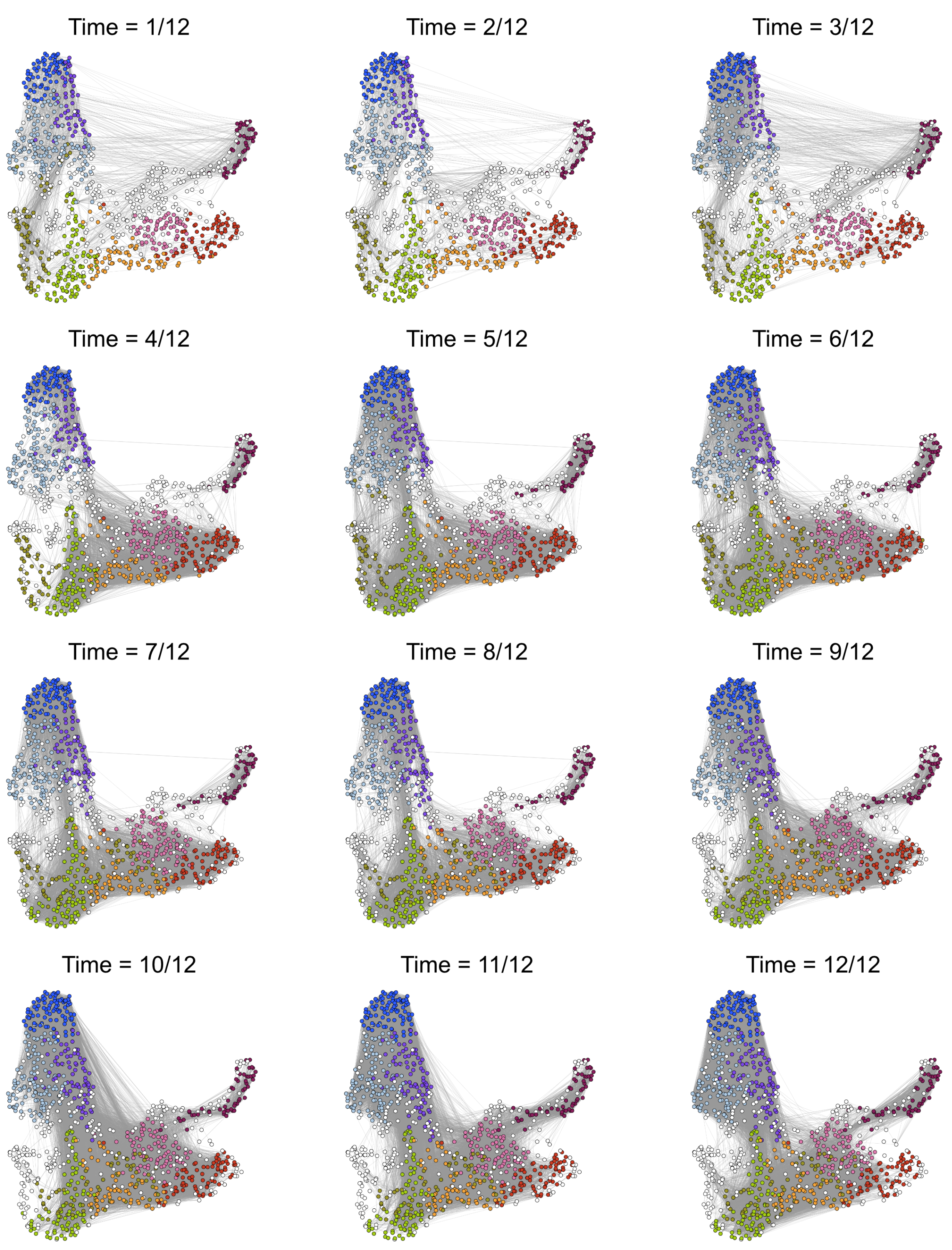
Figure figure: Gene memberships across all twelve networks, where the graphical layout is fixed, and the gray lines denote edges between two correlated genes. Each gene is colored one of ten different colors (community 1 as burgundy, community 2 as red, community 3 as salmon, community 4 as orange, community 5 as lime, community 6 as olive, community 7 as purple, community 8 as purple, community 9 as blue, and community 10 as white).

In Figure figure, we plot each of the twelve networks as adjacency matrices (i.e., heatmaps), where the genes are reshuffled from in rows/columns from one plot to the next so that genes in each community are grouped together. We can see an obvious membership structure within each network and slightly varying community sizes across time.

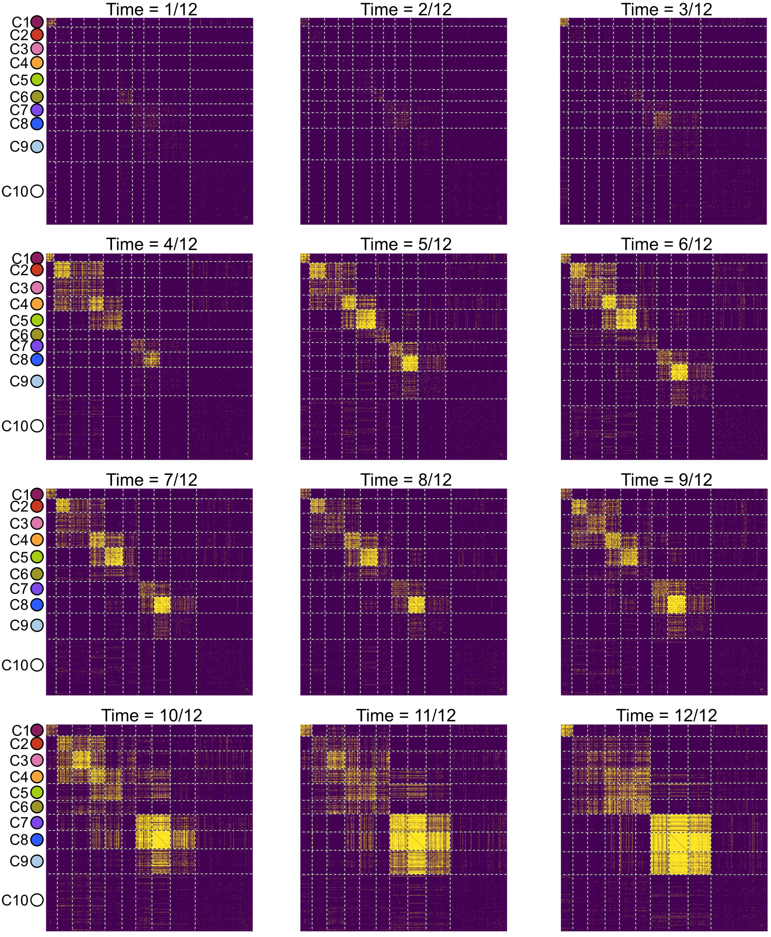
Figure figure: Adjacency matrices for each of the twelve networks, where the genes are reshuffled in rows/columns from one plot to the next so that genes in each community are grouped together. The yellow color denotes an edge between two genes, while dark blue denotes the absence of an edge. The communities are separated visually by a white dotted line. The colors for each community are the same as in figure.

In Figure figure, we plot the connectivity within and across communities, which better summarizes the adjacency matrices shown in Figure figure. Based on Sylvester’s criterion, we can see that some of the twelve networks are indefinite (i.e., contain negative eigenvalues) based on 2-by-2 submatrices along the diagonal that have negative eigenvalues.

Figure figure: Connectivity matrices as heatmaps for each of the twelve networks. The shown numbers denote the percentage of edges within or across communities (among all possible edges), and the colors range from white (i.e., connectivity of 0) to bright red (i.e., connectivity of 1). The colors for each community are the same as in figure.

Lastly, in Figure figure, we plot the alluvial plots demonstrating how the membership structure changes from one network to the next and how the 10-dimensional embedding is appropriate to reveal the community structure within each network. This is an extended version of Figure figure in the main text.

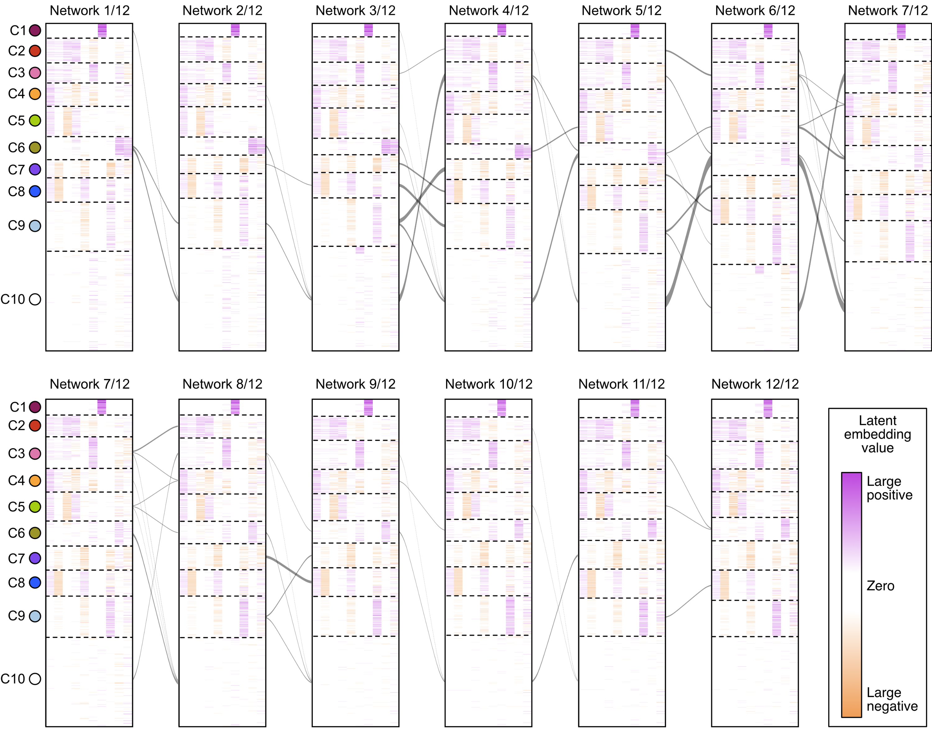
Figure figure: Alluvial plots across all twelve networks. This is an extension of the main text’s Figure figure. The colors for each community are the same as in figure.

References

- Abbe (2017) Abbe, E. (2017). Community detection and stochastic block models: Recent developments. The Journal of Machine Learning Research 18, 6446–6531.
- Arroyo et al. (2021) Arroyo, J., Athreya, A., Cape, J., Chen, G., Priebe, C. E. & Vogelstein, J. T. (2021). Inference for multiple heterogeneous networks with a common invariant subspace. Journal of Machine Learning Research 22, 1–49.
- Athreya et al. (2022) Athreya, A., Lubberts, Z., Park, Y. & Priebe, C. E. (2022). Discovering underlying dynamics in time series of networks. arXiv preprint arXiv:2205.06877 .
- Bhattacharyya & Chatterjee (2020) Bhattacharyya, S. & Chatterjee, S. (2020). General community detection with optimal recovery conditions for multi-relational sparse networks with dependent layers. arXiv preprint arXiv:2004.03480 .
- Bickel & Chen (2009) Bickel, P. J. & Chen, A. (2009). A nonparametric view of network models and newman–girvan and other modularities. Proceedings of the National Academy of Sciences 106, 21068–21073.
- Cai et al. (2018) Cai, T. T., Zhang, A. et al. (2018). Rate-optimal perturbation bounds for singular subspaces with applications to high-dimensional statistics. The Annals of Statistics 46, 60–89.
- Chen et al. (2020) Chen, S., Liu, S. & Ma, Z. (2020). Global and individualized community detection in inhomogeneous multilayer networks. arXiv preprint arXiv:2012.00933 .
- De la Pena & Giné (2012) De la Pena, V. & Giné, E. (2012). Decoupling: from dependence to independence. Springer Science & Business Media.
- Gallagher et al. (2021) Gallagher, I., Jones, A. & Rubin-Delanchy, P. (2021). Spectral embedding for dynamic networks with stability guarantees. arXiv preprint arXiv:2106.01282 .
- Han et al. (2015) Han, Q., Xu, K. & Airoldi, E. (2015). Consistent estimation of dynamic and multi-layer block models. In International Conference on Machine Learning. PMLR.
- Holland et al. (1983) Holland, P. W., Laskey, K. B. & Leinhardt, S. (1983). Stochastic blockmodels: First steps. Social networks 5, 109–137.
- Huang et al. (2018) Huang, M., Wang, J., Torre, E., Dueck, H., Shaffer, S., Bonasio, R., Murray, J. I., Raj, A., Li, M. & Zhang, N. R. (2018). SAVER: Gene expression recovery for single-cell RNA sequencing. Nature Methods 15, 539–542.
- Keriven & Vaiter (2022) Keriven, N. & Vaiter, S. (2022). Sparse and smooth: Improved guarantees for spectral clustering in the dynamic stochastic block model. Electronic Journal of Statistics 16, 1330–1366.
- Kim et al. (2018) Kim, B., Lee, K. H., Xue, L. & Niu, X. (2018). A review of dynamic network models with latent variables. Statistics surveys 12, 105.
- Lei et al. (2020) Lei, J., Chen, K. & Lynch, B. (2020). Consistent community detection in multi-layer network data. Biometrika 107, 61–73.
- Lei & Lin (2022) Lei, J. & Lin, K. Z. (2022). Bias-adjusted spectral clustering in multi-layer stochastic block models. Journal of the American Statistical Association , 1–13.
- Lei & Rinaldo (2015) Lei, J. & Rinaldo, A. (2015). Consistency of spectral clustering in stochastic block models. The Annals of Statistics 43, 215–237.
- Lei et al. (2023) Lei, J., Zhang, A. R. & Zhu, Z. (2023). Computational and statistical thresholds in multi-layer stochastic block models. arXiv preprint arXiv:2311.07773 .
- Liu et al. (2018) Liu, F., Choi, D., Xie, L. & Roeder, K. (2018). Global spectral clustering in dynamic networks. Proceedings of the National Academy of Sciences 115, 927–932.
- McInnes et al. (2018) McInnes, L., Healy, J. & Melville, J. (2018). UMAP: Uniform manifold approximation and projection for dimension reduction. arXiv preprint arXiv:1802.03426 .
- Paul & Chen (2020) Paul, S. & Chen, Y. (2020). Spectral and matrix factorization methods for consistent community detection in multi-layer networks. The Annals of Statistics 48, 230–250.
- Pelekis (2016) Pelekis, C. (2016). Lower bounds on binomial and poisson tails: an approach via tail conditional expectations. arXiv preprint arXiv:1609.06651 .
- Pensky & Zhang (2019) Pensky, M. & Zhang, T. (2019). Spectral clustering in the dynamic stochastic block model. Electronic Journal of Statistics 13, 678–709.
- Sarkar & Moore (2006) Sarkar, P. & Moore, A. W. (2006). Dynamic social network analysis using latent space models. Advances in neural information processing systems 18, 1145.
- Stewart & Sun (1990) Stewart, G. & Sun, J. (1990). Matrix perturbation theory, acad. Press, Boston MA .
- Street et al. (2018) Street, K., Risso, D., Fletcher, R. B., Das, D., Ngai, J., Yosef, N., Purdom, E. & Dudoit, S. (2018). Slingshot: Cell lineage and pseudotime inference for single-cell transcriptomics. BMC Genomics 19, 477.
- Trevino et al. (2021) Trevino, A. E., Müller, F., Andersen, J., Sundaram, L., Kathiria, A., Shcherbina, A., Farh, K., Chang, H. Y., Pașca, A. M., Kundaje, A., Pasca, S. P. & Greenleaf, W. J. (2021). Chromatin and gene-regulatory dynamics of the developing human cerebral cortex at single-cell resolution. Cell .
- Wang et al. (2021) Wang, D., Yu, Y. & Rinaldo, A. (2021). Optimal change point detection and localization in sparse dynamic networks. The Annals of Statistics 49, 203–232.
- Yang & Peng (2020) Yang, J. & Peng, J. (2020). Estimating time-varying graphical models. Journal of Computational and Graphical Statistics 29, 191–202.
- Yu et al. (2014) Yu, Y., Wang, T. & Samworth, R. J. (2014). A useful variant of the Davis–Kahan theorem for statisticians. Biometrika 102, 315–323.
Acknowledgement
We thank David Choi, Bernie Devlin, and Kathryn Roeder for useful comments when developing this method. Jing Lei’s research is partially supported by NSF grants DMS-2015492 and DMS-2310764.