TSSS: A Novel Triangulated Spherical Spline Smoothing

for Surface-based Data

Zhiling Gu^a, Shan Yu^b, Guannan Wang^c, Ming-Jun Lai^d and Li Wang^e

^aIowa State University, ^bUniversity of Virginia, ^cCollege of William & Mary,

^dUniversity of Georgia and ^eGeorge Mason University

Abstract: Surface-based data is commonly observed in diverse practical applications spanning various fields. In this paper, we introduce a novel nonparametric method to discover the underlying signals from data distributed on complex surface-based domains. Our approach involves a penalized spline estimator defined on a triangulation of surface patches, which enables effective signal extraction and recovery. The proposed method offers several advantages over existing methods, including superior handling of “leakage” or “boundary effects” over complex domains, enhanced computational efficiency, and potential applications in analyzing sparse and irregularly distributed data on complex objects. We provide rigorous theoretical guarantees for the proposed method, including convergence rates of the estimator in both the $L_{2}$ and supremum norms, as well as the asymptotic normality of the estimator. We also demonstrate that the convergence rates achieved by our estimation method are optimal within the framework of nonparametric estimation. Furthermore, we introduce a bootstrap method to quantify the uncertainty associated with the proposed estimators accurately. The superior performance of the proposed method is demonstrated through simulation experiments and data applications on cortical surface functional magnetic resonance imaging data and oceanic near-surface atmospheric data.

Key words and phrases: Complex domain; Nonparametric smoothing; Sphere-like surface; Spherical splines; Triangulation.

1 Introduction

Surface-based data is widely observed in various fields, and extracting useful information from data distributed on surfaces is of great significance. For example, in planetary science, scientists are interested in the movement of tectonic plates (Chang et al., 2000; Marzio et al., 2019) observed on the surfaces of celestial bodies. In cosmology, completing the missing data and correcting the noisy observations for the cosmic microwave background radiation are problems of interest (Abrial et al., 2008). In meteorology, hourly surface-based data is the most used and requested type of climatology data, and efforts have been made to integrate data from different stations across various repositories (Smith et al., 2011). Additional examples include the recovery of high-resolution time series of aerosol optical depth (Zhang et al., 2022b) and total electron content (Sun et al., 2022) from surface-based measurements.

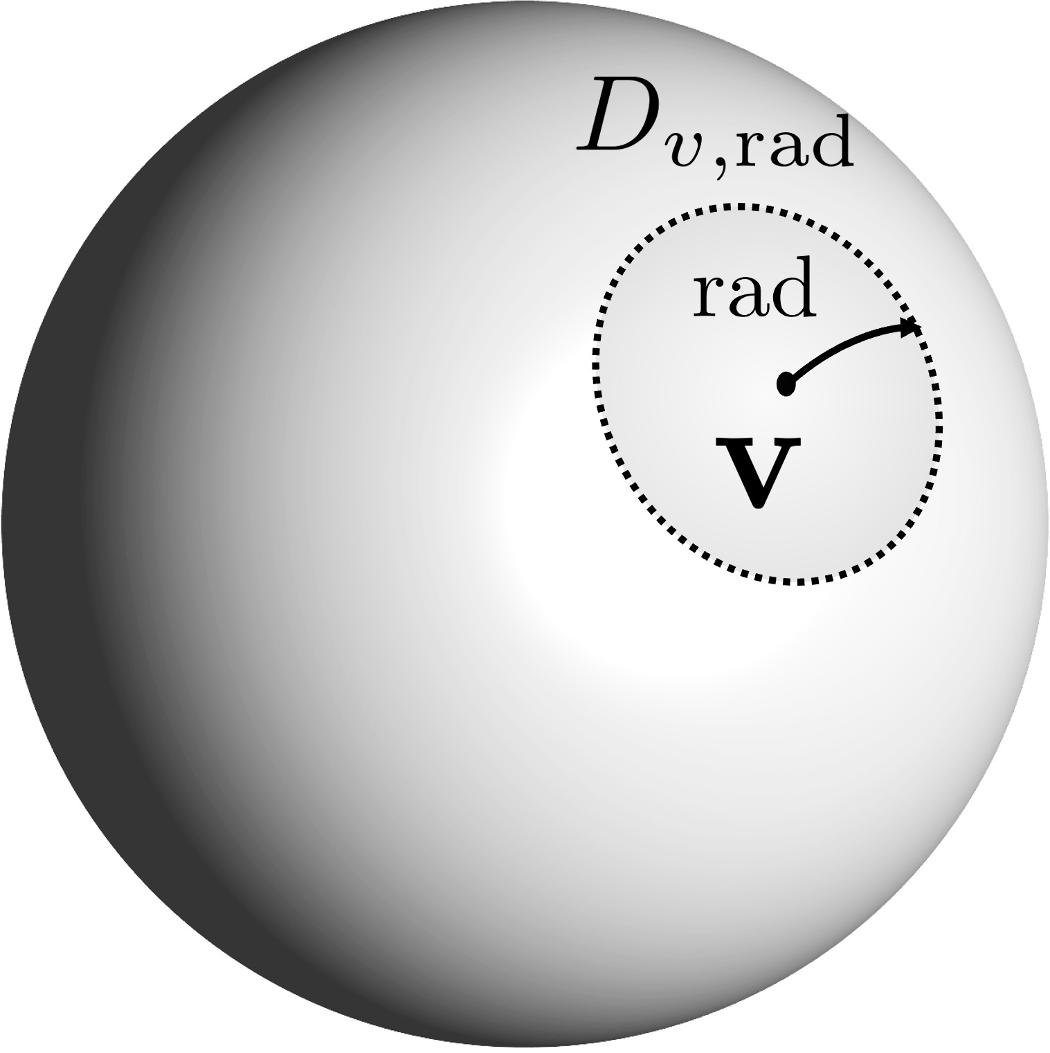
Furthermore, in biomedical research, efforts have been made to explore the functional properties of proteins using molecular surface data (Kinoshita and Nakamura, 2003). Another active area of investigation is cortical and cortical surface functional magnetic resonance imaging (fMRI) in neuroimaging. This technique offers the advantage of recovering anatomical structures with higher precision compared to volumetric fMRI methods (Brodoehl et al., 2020; Mejia et al., 2020; Lila and Aston, 2020; Cole et al., 2021; Zhang et al., 2022c). To analyze data distributed on general surfaces, it is common to employ mappings that project the data onto a unit sphere (Gu et al., 2004; Fischl et al., 1999), as depicted in Figure 1.

To model and denoise the spherical data, spherical harmonics (SH) (Seeley, 1966; Abrial et al., 2008) are widely used as global basis methods to interpolate functions on the whole sphere. Later, thin plate splines on the sphere (TPSOS) (Wahba, 1981) were proposed as a special case of SH while accounting for the smoothness of functions. However, in some instances, they may lack the desired flexibility needed to capture the complexity of the underlying signal accurately. SH relies on a fixed set of basis functions that span the entire sphere. While it has the ability to represent a wide range of functions, it may encounter challenges when dealing with highly localized or rapidly changing functions. A high number of basis functions is often required to achieve a good approximation power in such situations. This increased complexity can pose computational challenges and limit the practicality of using spherical harmonics. Similarly, TPSOS incorporates the concept of function smoothness but may still face difficulties when fitting complex functions. The flexibility of TPSOS is limited by its basis functions, which are constructed based on polynomial functions of trigonometric functions of longitudes and co-latitudes.

Another popular method is the kernel-based approach (Cao et al., 2013); however, it becomes computationally intensive for large datasets primarily due to the computation and storage requirements of kernel matrices and the need for solving optimization problems involving these matrices. The size of the kernel matrix is proportional to the number of data points, which makes the computation and storage requirements overgrow with the dataset size. The limitations of existing methods motivate the need for alternative methods that can offer enhanced flexibility in capturing the complexity of the underlying signal for spherical data.

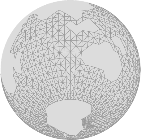
In addition, it is common for data to be collected over complex patches/regions of surfaces with irregular boundaries or holes, such as the domain of the oceans shown in Figure 2(e). It is well known that all aforementioned conventional tools for analyzing spherical data suffer from the problem of “leakage” across irregular-shaped domains due to inappropriately linking parts of the domain, as discussed in literature (Ramsay, 2002; Wood et al., 2008). Motivated by recent works, such as Lai and Wang (2013) and Wang et al. (2020a), Bernstein-Bézier polynomials defined on triangles are useful tools over planar domains with irregular shapes. Given the similarity and common properties between classical polynomial splines over planar triangulation and the spherical setting, spherical Bernstein-Bézier splines (Alfeld et al., 1996a, c) could be well suited for spherical data interpolation and approximation problems for complex sphere-like surfaces. The researchers in Baramidze and Lai (2005), Baramidze et al. (2006), Lai et al. (2008), and Baramidze and Lai (2011) have employed spherical Bernstein-Bézier splines for data interpolation and fitting, particularly in the context of geo-potential reconstruction, demonstrating their efficacy in modeling the geo-potential function. In this paper, we introduce a novel application of spherical splines specifically tailored to analyze data distributed on complex surface-based domains such as surface patches with complex boundaries. This innovative approach, referred to as triangulated spherical spline smoothing (TSSS), enables the extraction of underlying signals from intricate data structures on surface patches in the presence of noise. Our TSSS approach provides a robust and computationally efficient method for accurately estimating and modeling complex surface patterns.

Figure 1: Workflow of the TSSS estimation method for brain surface data.

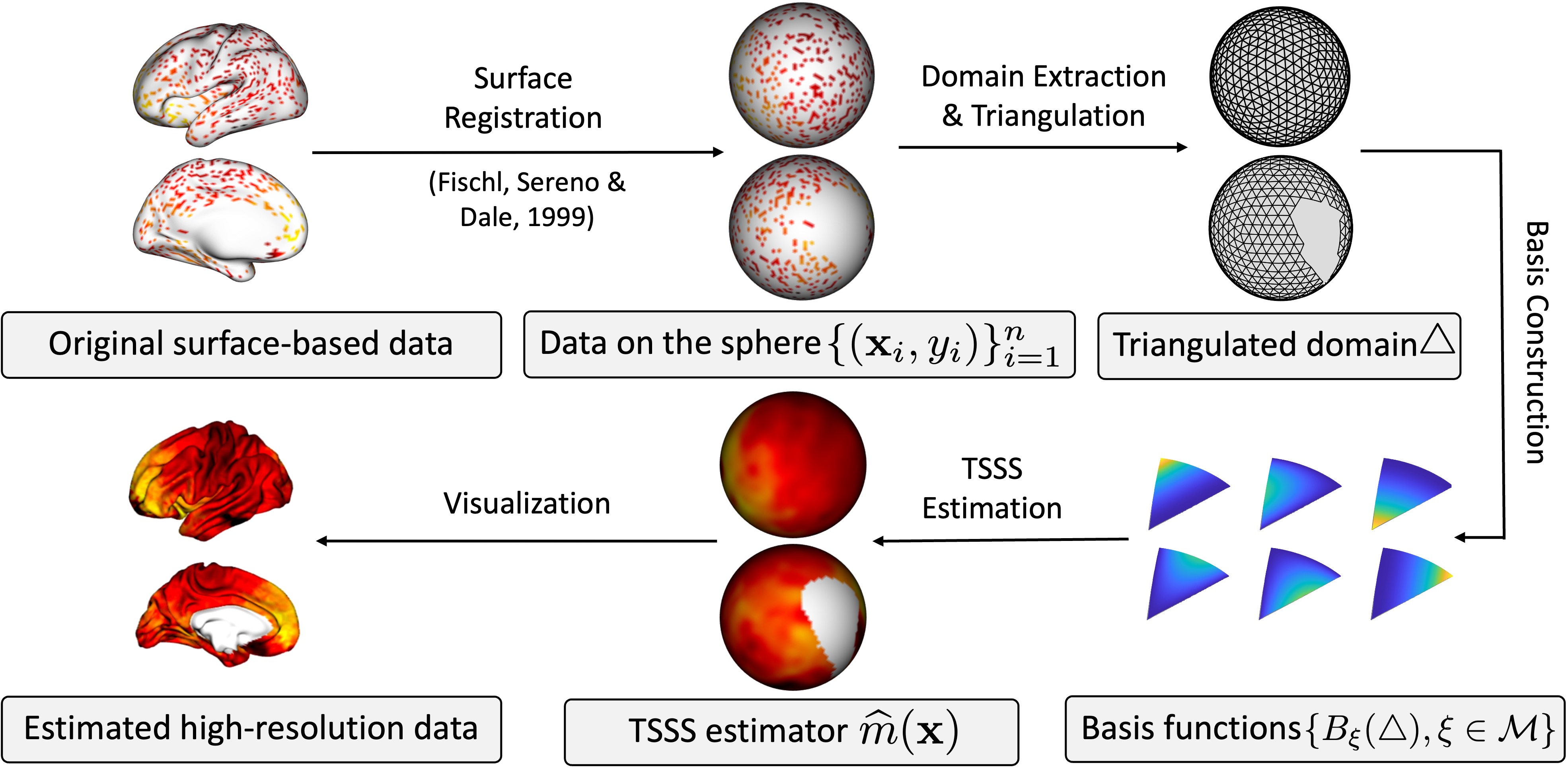
The proposed TSSS method overcomes the limitations of existing methods and offers several advantages. Firstly, it effectively addresses the problem of “leakage” across complex domains by utilizing information from neighboring triangles to accurately denoise or deblur data while preserving geometric features and spatial structures. This makes it ideal for analyzing data on complex patches or regions of surfaces with irregular boundaries or holes. Secondly, TSSS employs compactly supported basis functions and a sparse or roughness penalty, similar to P-splines (Eilers and Marx, 2021) and bivariate penalized splines on triangulation (BST; Lai and Wang, 2013; Yu et al., 2020a; Wang et al., 2023). This enables the model to capture intricate patterns in the data without becoming overly complex, mitigate boundary effects, and facilitate robust smoothing of unevenly distributed data, such as sparse and irregular data on surface-based complex domains. In addition, TSSS offers computational efficiency as a global estimation method with an explicit model expression. Its efficiency stems from the need to solve only a single linear system, which reduces the computational complexity and makes it suitable for handling large datasets.

Furthermore, we investigate the statistical properties of the proposed TSSS method. Specifically, we establish the convergence rate of the TSSS estimator, which is governed by the fineness of the triangle mesh, the spherical spline degree and smoothness, the penalty parameter, and the smoothness of the mean function. We further provide the conditions to achieve the optimal nonparametric convergence rate (Stone, 1982). We also derive the asymptotic normality for the TSSS estimator. However, due to the complexity of the spline basis functions, obtaining the exact form of the standard error can be challenging. Therefore, we propose a wild-bootstrap-based method to estimate the standard error.

The rest of this paper is organized as follows. Section 2 introduces the triangulation of a sphere and the spline space defined on the triangulation. In Section 3, we present the asymptotic properties of the proposed TSSS estimator, including convergence rates and asymptotic normality. Additionally, we introduce a bootstrap method to effectively quantify the uncertainty associated with the TSSS estimators. Section 4 outlines the implementation details of the TSSS method, including the selection of triangulation, spline basis, and penalty parameters. In Section 5, we present simulation studies to evaluate the finite sample performance of the TSSS estimator for functions observed on the grid of the whole sphere and functions observed on a complex spherical domain, and the uncertainty quantification of the TSSS estimators. In Section 6, TSSS is applied to cortical surface fMRI data and near-surface ocean-atmospheric data. Section 7 summarizes the main contributions of this paper and concludes with some remarks. Technical details are provided in the Supplementary Materials.

2 Penalized Spline Estimators on Triangulated Spheres

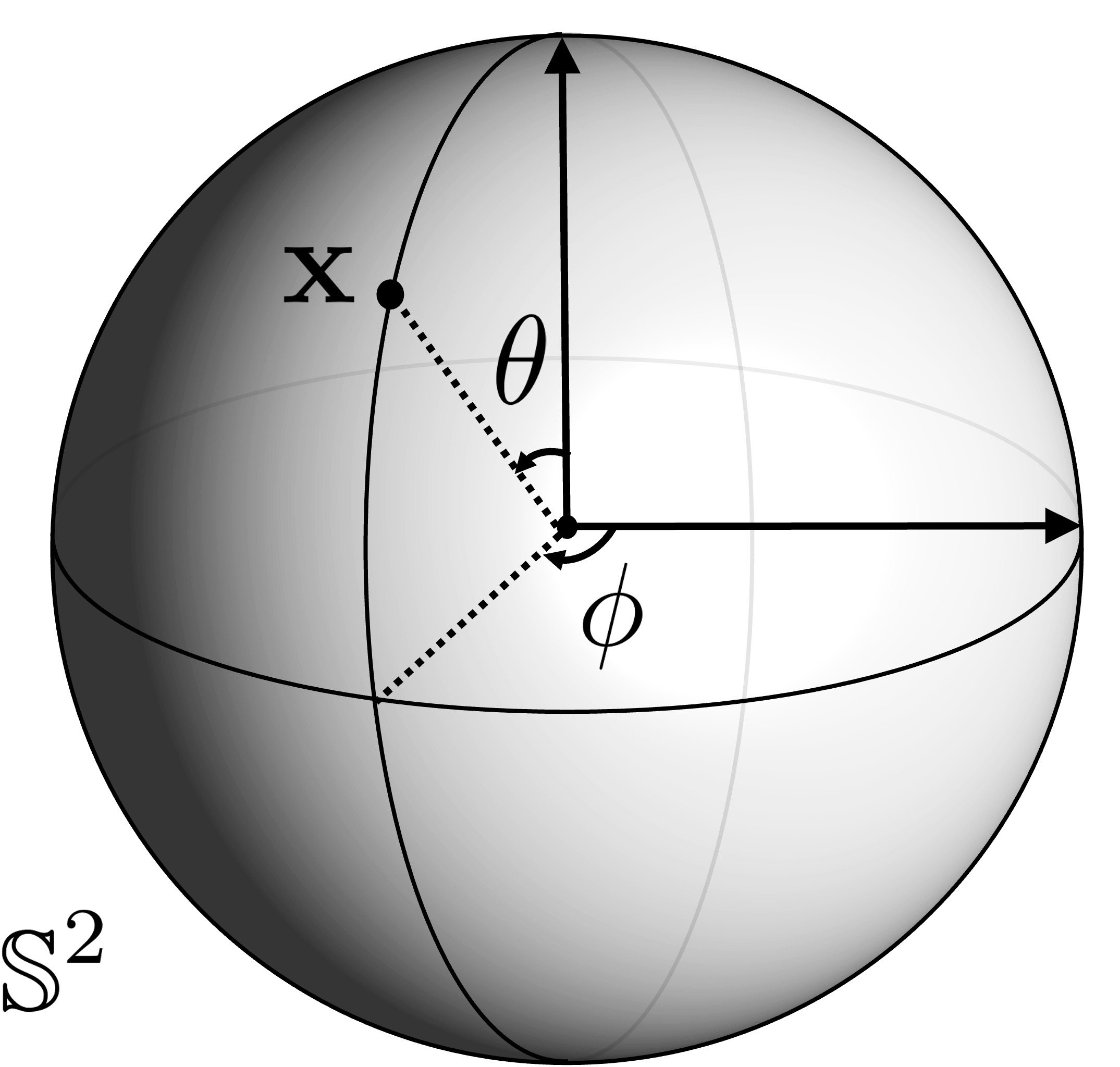
Consider a set of observations $\{(\theta_{i},\phi_{i},Y_{i})\}_{i=1}^{n}$, where $Y_{i}\in{\mathbb{R}}$ represents the response variable, $\theta_{i}\in[0,\pi]$ and $\phi_{i}\in[0,2\pi)$ denote the corresponding colatitude and longitude as illustrated in Figure 2(a). It is worth pointing out that a sphere $\mathbb{S}^{2}$ is a 2-dimensional (2D) object, which, for the convenience of analysis, is embedded in a 3-dimensional (3D) Euclidean space ${\mathbb{R}}^{3}$. Consequently, it is equivalent to consider any point on $\mathbb{S}^{2}$ in the following form $\mathbf{X}_{i}=(X_{i1},X_{i2},X_{i3})^{\top}\in{\mathbb{R}}^{3}$, where $\|\mathbf{X}_{i}\|_{2}^{2}=X_{i1}^{2}+X_{i2}^{2}+X_{i3}^{2}=1$. Suppose $\{(\mathbf{X}_{i},Y_{i}),\mathbf{X}_{i}\in\Omega\}_{i=1}^{n}$ is a i.i.d sample of size $n$ observed on a domain $\Omega$. Here, $\Omega$ can be either the entire unit spherical domain $\mathbb{S}^{2}$ or a specific spherical patch or region within $\mathbb{S}^{2}$. We assume the sample is drawn from the distribution of $(\mathbf{X},Y)$, $\mathbf{X}\in\Omega$, through

$$Y_{i}=m(\mathbf{X}_{i})+\sigma(\mathbf{X}_{i})\epsilon_{i},~{}i=1,2,\ldots,n,$$ (1)

where $m(\cdot)$ and $\sigma(\cdot)$ are the conditional mean and standard deviation functions, $\epsilon_{i}$’s are i.i.d random errors with mean ${\mathrm{E}}(\epsilon_{i})=0$, and variance $\mathrm{Var}(\epsilon_{i})=1$. In addition, we assume $\epsilon_{i}$ and $\mathbf{X}_{i}$ are independent for all $i$. The problem of interest is to estimate the unknown mean function $m(\mathbf{x})$ given observations $\{(\mathbf{X}_{i},Y_{i}),\mathbf{X}_{i}\in\Omega\}_{i=1}^{n}$.

2.1 Triangulation and Spherical Bernstein-Bézier polynomials

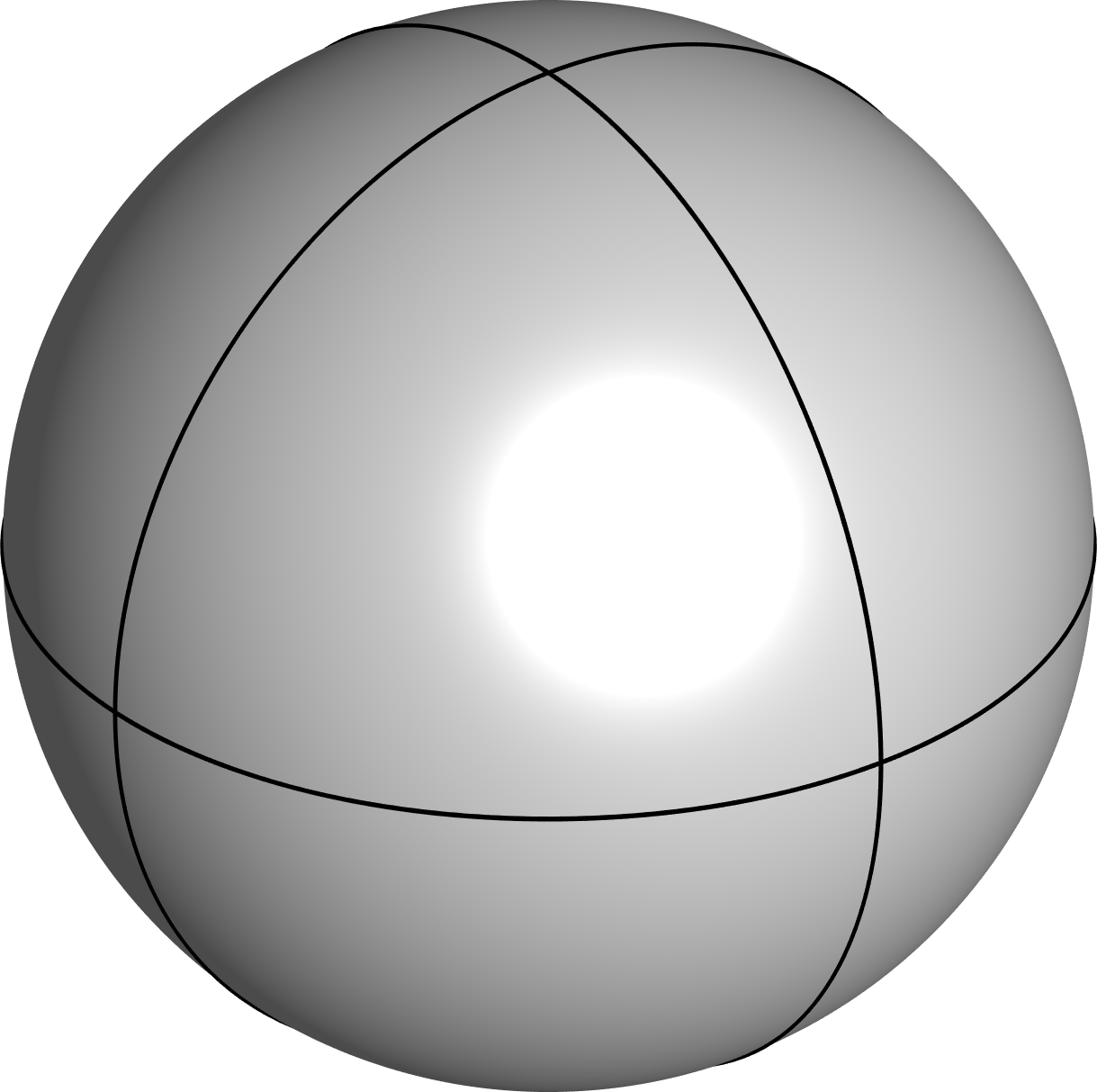
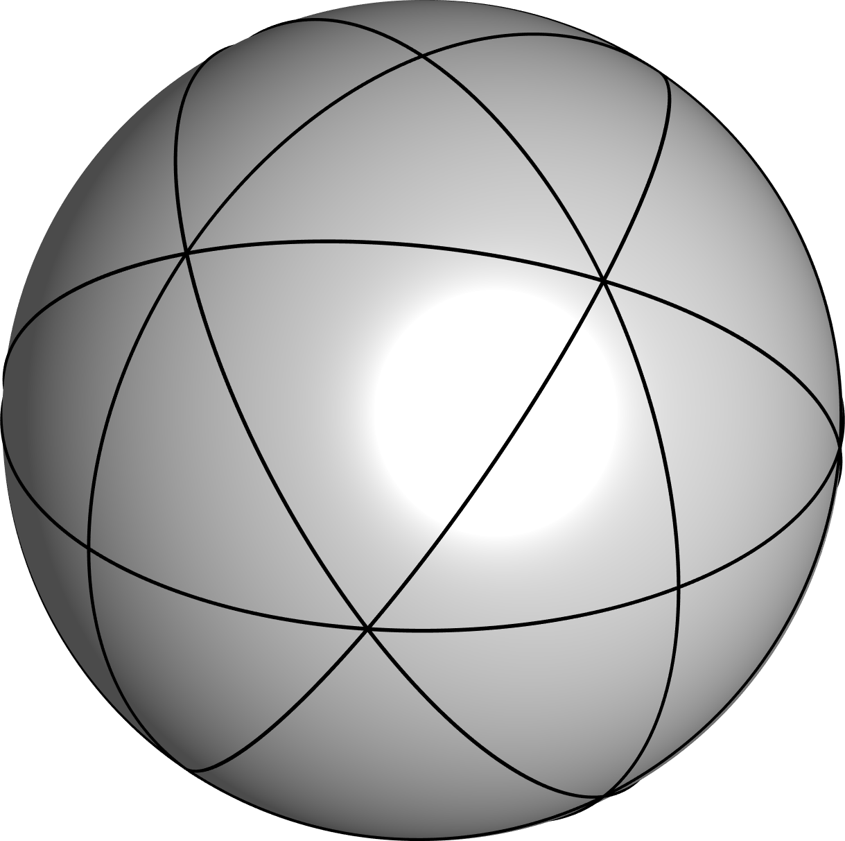
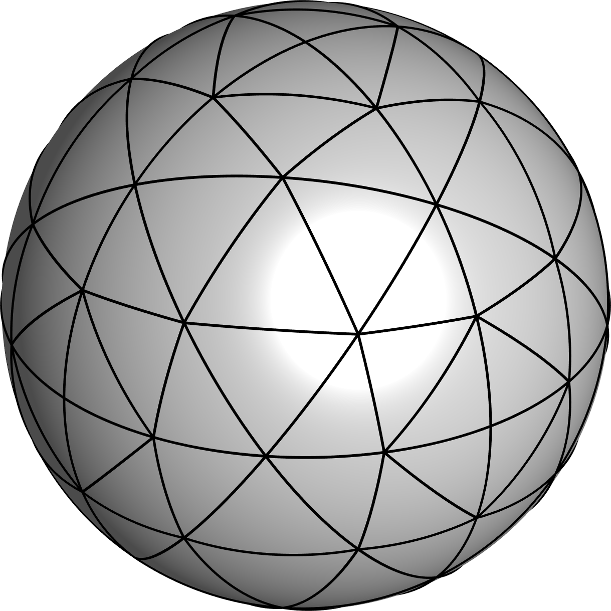
Triangulation has been widely used for irregular planar, spherical, and 3D domains due to its ability to effectively approximate complex geometries and simplify computational tasks (de Berg et al., 2008; Lai and Schumaker, 2007; De Loera et al., 2010). For domain $\Omega\subseteq\mathbb{S}^{2}$, a triangulation $\triangle$ is defined as a collection of $N$ spherical triangles $\triangle=\{\tau_{1},\ldots,\tau_{N}\}$, such that $\Omega=\cup_{i=1}^{N}\tau_{i}$ (Lai and Schumaker, 2007). Each spherical triangle $\tau:=\langle\mathbf{v}_{1},\mathbf{v}_{2},\mathbf{v}_{3}\rangle$ comprises the set of points in $\Omega$ that lie within the region bounded by three circular arcs $\langle\mathbf{v}_{i},\mathbf{v}_{i+1}\rangle,i=1,2,3$. Here $\mathbf{v}_{1},\mathbf{v}_{2},\mathbf{v}_{3}$ are the three vertices of $\tau$, and $\mathbf{v}_{4}$ is identified as $\mathbf{v}_{1}$. These spherical triangles either share an edge (circular arc), share a vertex, or do not intersect each other. Figure 2 provides an illustration of spherical triangulations.

(a)	(b)	(c)	(d)	(e)

Figure 2: Illustrations of (a) colatitude $\theta$ and longitude $\phi$, (b)-(d) spherical triangulations with varying levels of refinements, and (e) triangulation of the ocean surface. Refinement of the triangulation is achieved by connecting the center of each edge with the spherical edge with the shortest geodesic length.

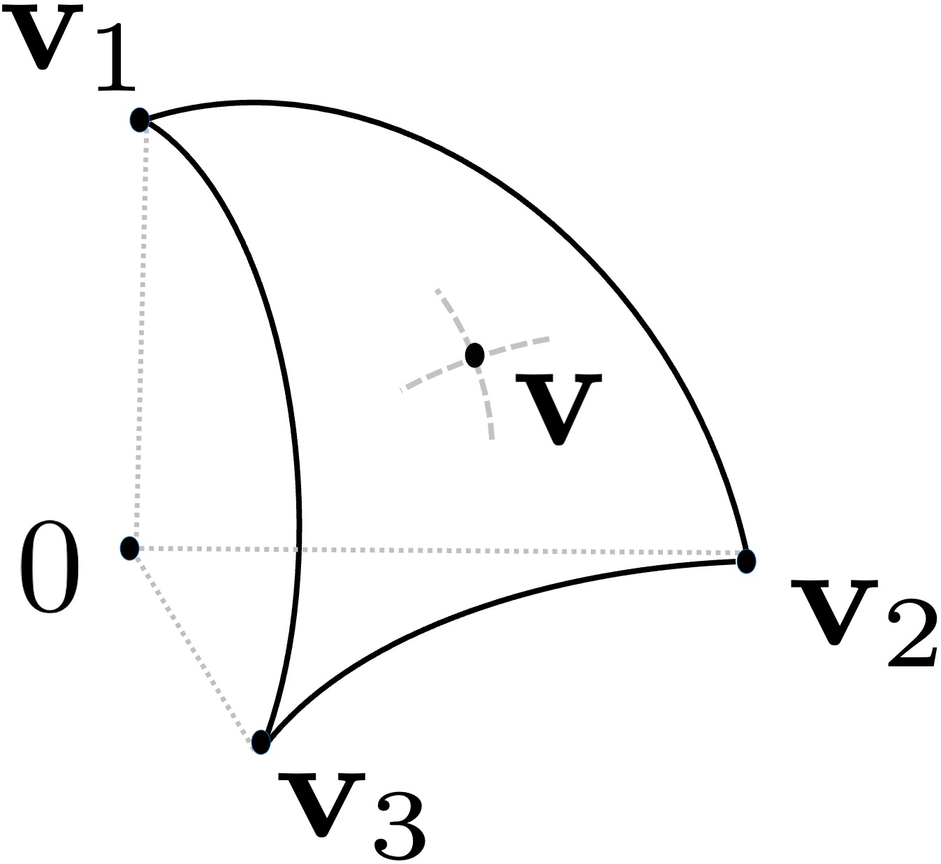
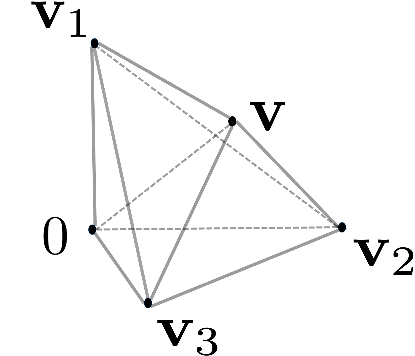
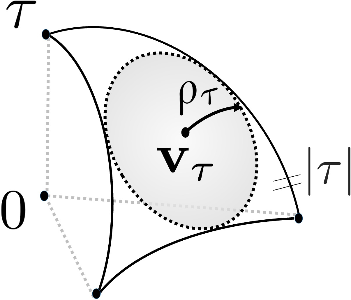
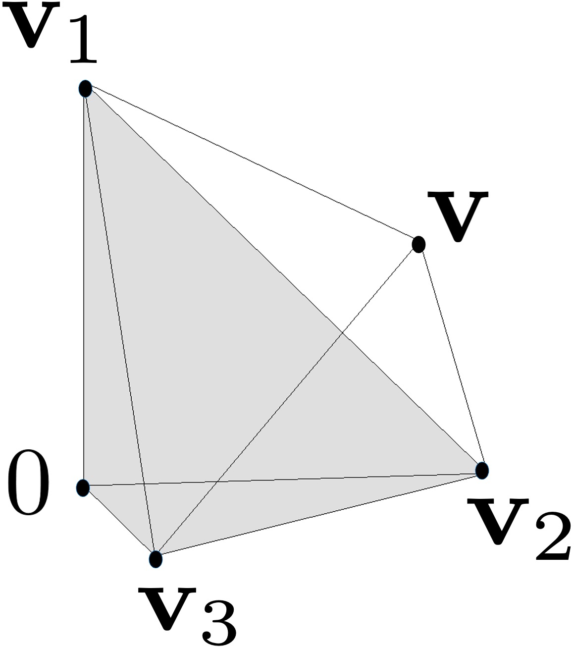
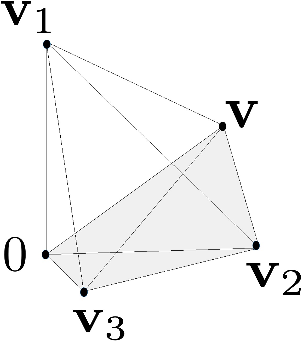
Further, we define the spherical barycentric coordinates $b_{1}(\mathbf{v}),b_{2}(\mathbf{v}),b_{3}(\mathbf{v})$ for any point $\mathbf{v}\in\mathbb{S}^{2}$ relative to a nondegenerate spherical triangle $\tau=\langle\mathbf{v}_{1},\mathbf{v}_{2},\mathbf{v}_{3}\rangle$, such that $\mathbf{v}=b_{1}(\mathbf{v})\mathbf{v}_{1}+b_{2}(\mathbf{v})\mathbf{v}_{2}+b_{3}(\mathbf{v})\mathbf{v}_{3}$. Note that $b_{\kappa}(\mathbf{v})=\mathrm{vol}(\uptau_{\kappa})/\mathrm{vol}(\uptau)$ is unique, where $\uptau_{\kappa}$ is tetrahedron $\langle\mathbf{0},\mathbf{v},\mathbf{v}_{\kappa+1},\mathbf{v}_{\kappa+2}\rangle$, and $\uptau$ is tetrahedron $\langle\mathbf{0},\mathbf{v}_{1},\mathbf{v}_{2},\mathbf{v}_{3}\rangle$. Here, $\mathbf{0}$ represents the center of a sphere; see Figure 3. This holds for $\kappa=1,2,3$, where $\mathbf{v}_{2}=\mathbf{v}_{5}$.

(a)	(b)	(c)	(d)

Figure 3: Illustrations of (a) a spherical triangle $\tau$, (b) tetrahedrons related to $\mathbf{v}$, (c) a spherical cap $D_{v,\mathrm{rad}}$, and (d) an inscribed cap of spherical triangle $\tau$.

For integers $d>r>0$, let $C^{r}(\Omega)$ denote the space of $r$-th continuously differentiable functions, and $\mathcal{H}_{d}$ represent the space of homogeneous trivariate polynomials of degree $d$ (Alfeld et al., 1996b). Following Baramidze et al. (2006) and Lai et al. (2008), we define the space of homogeneous spherical splines as $\mathcal{S}_{d}^{r}(\triangle)=\{s\in C^{r}(\Omega),s|_{\tau}\in\mathcal{H}_{d},\tau\in\triangle\}$, where $s|_{\tau}$ refers to the polynomial piece of spline $s$ restricted on triangle $\tau$. Using spherical barycentric coordinates, we can construct a basis for $\mathcal{H}_{d}$, called spherical Bernstein-Bézier (SBB) polynomials: $B_{ijk}^{\tau}(\mathbf{x})=\frac{d!}{i!j!k!}b_{1}(\mathbf{x})^{i}b_{2}(\mathbf{x})^{j}b_{3}(\mathbf{x})^{k}$, $i+j+k=d$, $\tau\in\triangle$. Consequently, any $s\in\mathcal{H}_{d}$ can be expressed as $s(\mathbf{x})=\sum_{\tau\in\triangle}\sum_{i+j+k=d}\gamma_{ijk}^{\tau}B_{ijk}^{\tau}(\mathbf{x})$, where $\gamma_{ijk}^{\tau}$’s are referred to as B-coefficients. Since $\gamma_{ijk}^{\tau}$’s are linearly independent, the dimension of $\mathcal{H}_{d}(\tau)$ is $(d+2)(d+1)/2$, as seen in Definition 13.17 of Lai and Schumaker (2007). Moreover, a stable local basis ${B_{\xi},\xi\in\mathcal{M}}$ for $\mathcal{S}_{d}^{r}(\triangle)$ can be constructed, with $\mathcal{M}$ being the index set of SBB bases. For more details, see Theorem 14.25 in Lai and Schumaker (2007), and refer to the Supplementary Material Section B.3. for detailed illustrations.

To describe the local properties of a domain on the sphere, we refer to the concept of “spherical cap” as introduced in Neamtu and Schumaker (2004). A spherical cap of radius $\mathrm{rad}$ associated with a point $\mathbf{v}\in\mathbb{S}^{2}$ is defined as the set of all points that has a geodesic distance to $\mathbf{v}$ at most $\mathrm{rad}$. For a spherical triangle $\tau\in\triangle$, we define the inscribed cap as the largest spherical cap contained within $\tau$. The center $\mathbf{v}_{\tau}$ of the inscribed cap is then referred to as the incenter of $\tau$, and the radius $\rho_{\tau}$ of the inscribed cap is denoted as the inradius of $\tau$. The longest spherical edge of $\tau$ is represented by $|\tau|$; see Figure 3. Denote by $|\triangle|=\max_{\tau\in\triangle}|\tau|$ the triangulation size corresponding to the longest spherical edge of all the triangles in $\triangle$. Let $\rho_{\triangle}$ denote the smallest inradius in $\triangle$, i.e., and $\rho_{\triangle}=\min_{\tau\in\triangle}\rho_{\tau}$. In addition, we define $A_{\tau}$ as the area of the spherical triangle $\tau$. To ensure all triangles in $\triangle$ have comparable sizes, we assume $\triangle$ satisfies Assumption (C2) described in Section 3 below.

2.2 Penalized spline estimators

In this section, we present a penalized spline estimator of the regression function $m(\cdot)$ in Model (1). To construct the penalized spline estimator, we first quantify the roughness of $f:\Omega\to{\mathbb{R}}$. Let $D^{\boldsymbol{\alpha}}f:=D_{x_{1}}^{i}D_{x_{2}}^{j}D_{x_{3}}^{k}f$ be a partial derivative of degree $|\boldsymbol{\alpha}|=i+j+k$ for $f$. The homogeneous extension of $f:\Omega\to{\mathbb{R}}$ of degree $p$, denoted as $f_{p}:{\mathbb{R}}^{3}\to{\mathbb{R}}$, is defined as

$$f_{p}(\mathbf{x}):=\|\mathbf{x}\|^{p}f(\mathbf{x}/\|\mathbf{x}\|),~{}\mathbf{x}\in{\mathbb{R}}^{3}\backslash\{\mathbf{0}\}$$ (2)

for any integer $p$, where $\|\mathbf{x}\|$ is the Euclidean norm of $\mathbf{x}$. We define energy functional of $f$ as

$$\mathcal{E}(f)=\sum_{|\boldsymbol{\alpha}|=2}\int_{\Omega}|D^{\boldsymbol{\alpha}}f_{p}|^{2}d\mu,$$ (3)

where $\mu$ is Lebesgue measure on $\mathbb{S}^{2}$ and the extended function $f_{p}$ is restricted to spherical domain $\Omega$ for integration. It is worth noting that any fixed value of $p$ can be chosen as the degree of extension. In our implementation, following Lai et al. (2008), we set $p=1$ for odd $d$ and $p=0$ for even $d$.

We propose the following Triangulated Spherical Spline Smoothing (TSSS) estimator for $m$, defined as the minimizer of the following objective function:

$$\widehat{m}_{\lambda}=\operatorname*{arg\,min}_{s\in\mathcal{S}_{d}^{r}(\triangle)}\sum_{i=1}^{n}\{Y_{i}-s(\mathbf{X}_{i})\}^{2}+\lambda\mathcal{E}(s),$$ (4)

where $\mathcal{S}_{d}^{r}(\triangle)$ is the space of homogeneous spherical splines defined in Section 2.1. The parameter $\lambda$ is a non-negative tuning parameter that balances the trade-off between the goodness of fit to the data and the smoothness of the estimate. Penalizing the energy functional with $\lambda\mathcal{E}(s)$ for some $\lambda>0$ reduces the roughness of the estimator, since higher values of $\mathcal{E}(s)$ indicate less smoothness.

Note that every function $s\in\mathcal{S}_{d}^{r}(\triangle)$ defined on a spherical triangle $\tau$ can be expressed as a linear combination of the SBB basis functions $\mathbf{B}^{\tau}(\mathbf{x})=(B_{\xi}^{\tau}(\mathbf{x}),\xi\in\mathcal{M})^{\top}$ using the coefficients $\boldsymbol{\gamma}^{\tau}=(\gamma_{\xi}^{\tau},\xi\in\mathcal{M})^{\top}$. Specifically, for any point $\mathbf{x}\in\tau$, we have $s(\mathbf{x})=\boldsymbol{\gamma}^{\tau\top}\mathbf{B}^{\tau}(\mathbf{x})$. Then, the energy functional $\mathcal{E}(s)$ in (3) can be rewritten as

$$\mathcal{E}(s)=\sum_{\tau\in\triangle}\int_{\tau}\left\{\diamondsuit(\boldsymbol{\gamma}^{\tau\top}\mathbf{B}^{\tau}(\mathbf{x}))\right\}^{\otimes 2}d\mu=\sum_{\tau\in\triangle}\int_{\tau}\boldsymbol{\gamma}^{\tau\top}\left\{\diamondsuit(\mathbf{B}^{\tau}(\mathbf{x}))\right\}^{\otimes 2}\boldsymbol{\gamma}^{\tau}d\mu,$$ (5)

where $\diamondsuit f:=(D^{\boldsymbol{\alpha}}f_{p},|\boldsymbol{\alpha}|=2)$ is the second order derivative vector of $f\in\mathcal{S}$ given in (2), $\mathbf{x}^{\otimes 2}=\mathbf{x}\mathbf{x}^{\top}$.

Since the spline coefficients of $s\in{\cal{C}}^{r}(\triangle)$ need to satisfy some smoothness conditions across each interior face of $\triangle$, a smoothness constraint matrix $\mathbf{M}$ can be used to impose the required smoothness. Specifically, $\mathbf{M}\boldsymbol{\gamma}=\boldsymbol{0}$ is imposed as a smoothness condition to ensure that the estimated function is $r$-th differentiable on all edges of $\triangle$. By doing so, the smoothness of the TSSS estimator can be controlled and achieved for different values of $r$. For spline function $\mathbf{B}(\mathbf{x})^{\top}\boldsymbol{\gamma}$ we have $\mathcal{E}(\mathbf{B}^{\top}\boldsymbol{\gamma})=\boldsymbol{\gamma}^{\top}\mathbf{P}\boldsymbol{\gamma}$, where $\mathbf{P}$ is a $\{N(d+1)(d+2)/2\}\times\{N(d+1)(d+2)/2\}$ block diagonal penalty matrix and can be obtained from (5). Thus, one can estimate the spline coefficients via minimizing

$$\widehat{\boldsymbol{\gamma}}=\operatorname*{arg\,min}_{\boldsymbol{\gamma}}\sum_{i=1}^{n}\{Y_{i}-\mathbf{B}(\mathbf{X}_{i})^{\top}\boldsymbol{\gamma}\}^{2}+\lambda\boldsymbol{\gamma}^{\top}\mathbf{P}\boldsymbol{\gamma},\mathrm{~{}subject~{}to~{}}\mathbf{M}\boldsymbol{\gamma}=\mathbf{0}.$$

Then, we can obtain the TSSS estimator by $\widehat{m}_{\lambda}(\mathbf{x})=\mathbf{B}^{\top}(\mathbf{x})\widehat{\boldsymbol{\gamma}}$.

3 Theoretical Results

To discuss the asymptotics of the TSSS estimator, we first introduce some technical notations. Let $X_{n}$, $n\geq 1$, be a sequence of random variables. We denote $X_{n}=O_{p}(a_{n})$ if $\lim_{c\to\infty}\limsup_{n\to\infty}P(|X_{n}|\geq ca_{n})=0$. Similarly, we write $X_{n}=o_{p}(a_{n})$ if $\lim_{n\to\infty}P(|X_{n}|\geq ca_{n})=0$ holds for any positive constant $c$. In addition, we denote $a_{n}\asymp b_{n}$ if there exists two positive constants $c$ and $C$ such that $c|a_{n}|\leq|b_{n}|\leq C|a_{n}|$. These notations are useful in discussing the rate of convergence and consistency of the TSSS estimator below.

For any measurable functions $f,f_{1},f_{2}$ defined over the closure of $\Omega\subseteq\mathbb{S}^{2}$, we define the theoretical and empirical inner products: $\langle f_{1},f_{2}\rangle_{\Omega}={\mathrm{E}}\{f_{1}(\mathbf{X})f_{2}(\mathbf{X})\}$, $\langle f_{1},f_{2}\rangle_{n,\Omega}=n^{-1}\sum_{i=1}^{n}f_{1}(\mathbf{X}_{i})f_{2}(\mathbf{X}_{i})$, respectively, with induced norms $\|f\|_{\Omega}=\{\langle f,f\rangle_{\Omega}\}^{1/2}$ and $\|f\|_{n,\Omega}=\{\langle f,f\rangle_{n,\Omega}\}^{1/2}$. We define the supremum norm $\|f\|_{\infty,\Omega}=\sup_{\mathbf{x}\in\Omega}|f(\mathbf{x})|$ and the $L^{q}$-norm $\|f\|_{L^{q}(\Omega)}=\{\int_{\Omega}|f(\mathbf{x})|^{q}d\mathbf{x}\}^{1/q}$. Furthermore, denote $\langle f_{1},f_{2}\rangle_{\mathcal{E}}=\sum_{\tau\in\triangle}\int_{\tau}(\diamondsuit f_{1,p})^{\top}\diamondsuit f_{2,p}d\mu$, where $\diamondsuit f=(D^{\boldsymbol{\alpha}}f_{p},|\boldsymbol{\alpha}|=2)^{\top}$ refers to the second-order partial derivatives of $f$.

Lemmas 1-2 presented below provide the relationships between the inner products and norms defined above. We first state some technical assumptions.

1. The density function of $\mathbf{X}$, $f_{\mathbf{X}}(\cdot)$, is bounded away from zero and infinity over $\Omega$.

2. For any spherical triangle $\tau$ within $\triangle$, it is contained in a spherical cap of radius $1/6$. The minimal determining set has constant $\curlywedge=3$; see Supplementary Material Section B.5.. Assume triangulation $\triangle$ is $\varrho$-quasi-uniform, that is, there exists a positive constant $\varrho$ such that $|\triangle|/\rho_{\tau}\leq\varrho$, for all $\tau\in\triangle$.

3. The number of triangles $N$ and sample size $n$ satisfy $N=Cn^{\omega}$ for some $C>0$ and $0<\omega<\eta/(\eta+2)$, where $\eta$ is defined in (C5).

Assumptions (C1)–(C3) are standard in nonparametric literature (Huang, 2003; Lai and Wang, 2013; Yu et al., 2020b). Assumption (C2) suggests the use of more uniform triangulations with smaller shape parameters (Baramidze and Lai, 2011). Assumption (C3) can be handled via the adjustment of triangulation. Considering the area of domain $\Omega$ as fixed, we can interchange $N$ and $|\triangle|^{-2}$ in all results.

Lemma 1.

Let $\{B_{\xi}\}_{\xi\in\mathcal{M}}$ be the basis for $\mathcal{S}_{d}^{r}(\triangle)$. Let $p_{1}=\sum_{\xi\in\mathcal{M}}\gamma^{(1)}_{\xi}B_{\xi}$, $p_{2}=\sum_{\xi\in\mathcal{M}}\gamma^{(2)}_{\xi}B_{\xi}$. Under Assumptions (C1) and (C3), we have

$$R_{n}=\sup_{p_{1},p_{2}\in\mathcal{S}_{d}^{r}(\triangle)}\left|\frac{\langle p_{1},p_{2}\rangle_{n,\Omega}-\langle p_{1},p_{2}\rangle_{\Omega}}{\|p_{1}\|_{\Omega}\|p_{2}\|_{\Omega}}\right|=O_{p}\left\{(N\log n)^{1/2}n^{-1/2}\right\}.$$

Lemma 2.

Under Assumptions (C1)–(C3), we have

$$V_{n}\!=\!\!\sup_{p\in S_{d}^{r}(\triangle)}\!\!\left\{\frac{\|p\|_{\infty,\Omega}}{\|p\|_{n,\Omega}},\|p\|_{n,\Omega}\neq 0\right\}{=O_{p}(\sqrt{N})},\bar{V}_{n}\!=\!\!\sup_{p\in S_{d}^{r}(\triangle)}\!\!\left\{\frac{\|p\|_{\mathcal{E}}}{\|p\|_{n,\Omega}},\|p\|_{n,\Omega}\neq 0\right\}{=O_{p}(N).}$$

3.1 Convergence Rate of TSSS Estimator

Before presenting the convergence results of the TSSS estimator, it is important to discuss the construction of the spherical Sobolev space and its related norms. The convergence rate of the estimator depends on the smoothness of the underlying regression function, and understanding the properties of the spherical Sobolev space is essential for understanding this relationship.

For an open set $\bar{\Omega}\subseteq\mathbb{R}^{2}$, let $W^{\ell}_{q}(\bar{\Omega})$ denote the classical Sobolev space as in Section 1.6 of Lai and Schumaker (2007), and $\|f\|_{W^{\ell}_{q}(\bar{\Omega})}=\sup_{|{\boldsymbol{\alpha}}|=\ell}\|D^{{\boldsymbol{\alpha}}}f\|_{L^{q}(\bar{\Omega})}$ denote the classical Sobolev norm. To work on an appropriate space for functions defined on $\Omega\subseteq\mathbb{S}^{2}$, we consider the following Sobolev space on the sphere $W^{\ell}_{q}(\Omega):=\left\{f:(\alpha_{j}^{*}f)\circ\phi_{j}^{-1}\in W^{\ell}_{q}(\bar{\Omega}_{j}),\forall j\right\},\,\ell>0$, where $f:\Omega\to\mathbb{R}$ is a spherical function; $\phi_{j}^{-1}:\mathbb{R}^{2}\to{\mathbb{S}^{2}}$ is a smooth mapping; $\bar{\Omega}_{j}\subseteq\mathbb{R}^{2}$ is an open set and the support of $\phi_{j}^{-1}$; and $\alpha_{j}^{*}:{\mathbb{S}^{2}}\to\mathbb{R}$ is a mapping to indicate the partition of $\mathbb{S}^{2}$. Thus, $(\alpha_{j}^{*}f)$ and $\phi_{j}^{-1}$ bridge $\mathbb{R}^{2}$ and $\mathbb{R}$, and induce the spherical Sobolev norm $\|f\|_{\ell,q,\Omega}=\sum_{j}\|(\alpha_{j}^{*}f)\circ\phi_{j}^{-1}\|_{W^{\ell}_{q}(\bar{\Omega}_{j})}$ for $\ell>0$. In addition, the spherical Sobolev seminorm is defined as $|f|_{\ell,q,\Omega}=\sum_{|{\boldsymbol{\alpha}}|=\ell}\|D^{{\boldsymbol{\alpha}}}f_{\ell-1}\|_{L^{q}(\Omega})$, where $\|D^{\boldsymbol{\alpha}}f_{\ell-1}\|_{L^{q}(\Omega)}$ is the $L^{q}$-norm of the extended trivariate function $f_{\ell-1}$ restricted to $\Omega$. When $\ell=0,$ the seminorm $|f|_{0,q,\Omega}$ reduces to $L^{q}$-norm $\|f\|_{L^{q}(\Omega)}$.

We introduce two additional assumptions.

1. The spherical mean function $m\in W^{\ell+1}_{q}(\Omega)$ for some integer $0\leq\ell\leq d,\ell=d(\mathrm{mod}2)$.

2. The noise $\epsilon$ satisfies $\lim_{\eta\to\infty}{\mathrm{E}}\{\epsilon^{2}I(\epsilon>\eta)\}=0$, and ${\mathrm{E}}|\epsilon_{i}^{2+\eta}|\leq v_{\eta}$, $\eta>0$. The standard deviation function $\sigma(\mathbf{x})$ is continuous, and $0<c_{\sigma}\leq\inf_{\mathbf{x}\in\Omega}\sigma(\mathbf{x})\leq\sup_{\mathbf{x}\in\Omega}\sigma(\mathbf{x})\leq C_{\sigma}<\infty$.

Assumption (C4) specifies the degree of smoothness required for $m$ (Baramidze and Lai, 2005, 2011). By characterizing the smoothness of the function using the Sobolev space and its norms, we can obtain the convergence rate of the estimator for different smoothness levels of the regression function. Assumption (C5) places constraints on the behavior of the noise and the standard deviation function, which helps establish the asymptotic normality of the TSSS estimator (Huang, 2003; Lai and Wang, 2013).

Define $s_{\lambda,m}$ and $s_{\lambda,\epsilon}$ as the penalized spline estimators based on $\{m(\mathbf{X}_{i})\}_{i=1}^{n}$ and $\{\sigma(\mathbf{X}_{i})\epsilon_{i}\}_{i=1}^{n}$, respectively. Let $\mathbb{B}=\sum_{i=1}^{n}\mathbf{B}(\mathbf{X}_{i})\mathbf{B}(\mathbf{X}_{i})^{\top}$, then

$$s_{\lambda,m}(\mathbf{x}) =\mathbf{B}(\mathbf{x})^{\top}\boldsymbol{\gamma}_{\lambda,m},~{}\boldsymbol{\gamma}_{\lambda,m}=\left(\mathbb{B}+\lambda\mathbf{P}\right)^{-1}\sum_{i=1}^{n}\mathbf{B}(\mathbf{X}_{i})m(\mathbf{X}_{i}),$$ (6)

$$s_{\lambda,\epsilon}(\mathbf{x}) =\mathbf{B}(\mathbf{x})^{\top}\boldsymbol{\gamma}_{\lambda,\epsilon},~{}\boldsymbol{\gamma}_{\lambda,\epsilon}=\left(\mathbb{B}+\lambda\mathbf{P}\right)^{-1}\sum_{i=1}^{n}\mathbf{B}(\mathbf{X}_{i})\sigma(\mathbf{X}_{i})\epsilon_{i}.$$ (7)

To evaluate the bias and variance of the proposed estimator, we decompose the estimation error as follows: $\widehat{m}_{\lambda}(\mathbf{x})-m(\mathbf{x})=\{s_{\lambda,m}(\mathbf{x})-m(\mathbf{x})\}+s_{\lambda,\epsilon}(\mathbf{x})$, where the first term represents the size of bias and the second term represents the size of variance in the estimation. The following propositions provide bounds for the order of the bias and variance terms.

Proposition 1.

Under Assumptions (C1)–(C4), if $d\geq 3r+2$ and $\triangle$ is a spherical triangulation such that $|\triangle|<1/6$, then we have the following uniform convergence rate: $\|s_{\lambda,m}-m\|_{\infty,\Omega}=O_{p}\{\lambda n^{-1}N^{3/2}|m|_{2,\infty,\Omega}+(1+\lambda n^{-1}N^{5/2})N^{-(\ell+1)/2}|m|_{\ell+1,\infty,\Omega}\}$.

Proposition 2.

Under Assumptions (C1)–(C3) and (C5), we have ${\|s_{\lambda,\epsilon}\|_{L^{2}(\Omega)}=O_{p}(n^{-1/2}N^{1/2})}$ and ${\|s_{\lambda,\epsilon}\|_{\infty,\Omega}=O_{p}\{n^{-1/2}(N\log n)^{1/2}+\lambda n^{-3/2}N^{3}\}}$.

Combining Propositions 1 and 2, we can obtain the following convergence rates of the TSSS estimator in terms of both $L^{2}$ and supremum norms in Theorem 1. These convergence rates are important for assessing the performance of the TSSS estimator under different smoothness assumptions and for guiding the choice of the triangulation and spline basis functions.

Theorem 1.

Under Assumptions (C1)–(C5), we have

$$\|\widehat{m}_{\lambda}-m\|_{L^{2}(\Omega)}= O_{p}\left\{\frac{\lambda N^{3/2}}{n}|m|_{2,\infty,\Omega}+\left(1+\frac{\lambda{N^{5/2}}}{n}\right)N^{-(\ell+1)/2}|m|_{\ell+1,\infty,\Omega}+{\sqrt{\frac{N}{n}}}\right\},$$

$$\|\widehat{m}_{\lambda}-m\|_{\infty,\Omega}= O_{p}\left\{\frac{\lambda{N^{3/2}}}{n}|m|_{2,\infty,\Omega}+\left(1+\frac{\lambda{N^{5/2}}}{n}\right)N^{-(\ell+1)/2}|m|_{\ell+1,\infty,\Omega}\right.$$

$$\hskip 199.16928pt\left.+{\sqrt{\frac{{N}\log n}{n}}+\frac{\lambda{N^{3}}}{n^{3/2}}}\right\}.$$

According to Theorem 1, the convergence rate of the TSSS estimators depends on sample size, triangulation size, and the roughness penalty parameter, as well as the characteristics of the underlying signal being estimated. The first and the third terms in the order of $\|\widehat{m}_{\lambda}-m\|_{L^{2}(\Omega)}$ and $\|\widehat{m}_{\lambda}-m\|_{\infty,\Omega}$ show the bias brought by the roughness penalty. When the tuning parameter is small enough, the second term in the order of $\|\widehat{m}_{\lambda}-m\|_{L^{2}(\Omega)}$ and $\|\widehat{m}_{\lambda}-m\|_{\infty,\Omega}$ represent the bias when approximating an arbitrary function $m$ by a spherical spline. The last two terms are the estimation variance generated from the random noise.

Theorem 1 also provides a guideline on how to choose the triangulation. As the sample size increases, a finer triangulation can be considered for a more accurate estimation of the mean function. In addition, a finer triangulation is needed when there are rapid changes in the mean function or when the domain is highly curved or complex. A more detailed discussion of triangulation selection is given in Section 4.

It can be demonstrated that the TSSS estimator achieves the optimal convergence rate under certain regularity conditions. As indicated in Stone (1982), the optimal global approximation rate for a nonparametric estimator can be expressed as follows: for the $L^{q}$-norm ($0<q<\infty$) of the approximation error, the rate is $n^{-r^{*}}$, where $r^{*}=p^{*}/(2p^{*}+d^{*})$, for a $p^{*}$-times differentiable function of a $d^{*}$-dimensional measurement variable; for $q=\infty$, the optimal convergence rate becomes $(n^{-1}\log n)^{r^{*}}$. In the case of our problem, where $\mathbf{x}\in\Omega\subseteq\mathbb{S}^{2}$, we have $d^{*}=2$. Furthermore, the mean function $m\in W_{q}^{\ell+1}(\triangle)$ implies that it is $p^{*}=(\ell+1)$-times differentiable. Therefore, the optimal global approximation rate is $n^{-(\ell+1)/(2\ell+4)}$ when $0<q<\infty$, and $(n/\log n)^{-(\ell+1)/(2\ell+4)}$ when $q=\infty$. When $\lambda=0$, the TSSS achieves the optimal convergence rate in $L^{2}$-norm when the number of triangles satisfies the condition $N\asymp n^{1/(\ell+2)}$, and it achieves the optimal convergence rate in the supremum norm when ${N\asymp(n/\log n)^{1/(\ell+2)}}$. When $\lambda>0$, the optimal convergence rate in $L^{2}$-norm is achieved under the conditions ${\lambda=O\{n^{\ell/(2\ell+4)}\}}$ and $N\asymp n^{1/(\ell+2)}$ . Furthermore, when ${\lambda=o\{n^{\ell/(2\ell+4)}\}}$ and $N\asymp(n/\log n)^{1/(\ell+2)}$, the TSSS estimator achieves the optimal convergence rate in the supremum norm.

3.2 Asymptotic Normality

To derive the asymptotic distribution of the TSSS estimator, we further assume the following:

1. The number of spherical triangles $N=Cn^{\omega}$, for some $C>0$ and $1/(\ell+2)<\omega<\eta/(\eta+2)$.

1. The roughness parameter satisfies that $\lambda=o(n^{1/2}N^{-1}\wedge nN^{-2})$.

Compared with Assumption (C3) in Section 3.1, (C5’) further assumes that the number of spherical triangles needs to be greater than a lower bound, which depends on the degree of the function. A similar assumption for the univariate case and bivariate case has been discussed (Li and Ruppert, 2008; Lai and Wang, 2013). Meanwhile, Assumption (C6) requires smaller $\lambda$, which reduces the bias through undersmoothing.

Theorem 2 below states the asymptotic normality of the proposed TSSS estimator.

Theorem 2.

Under Assumptions (C1),(C2), (C4), (C5), (C5’) and (C6), as $n\to\infty$, for each $\mathbf{x}\in\Omega$, $\left[{\rm Var}\left\{\widehat{m}_{\lambda}(\mathbf{x})|\mathbb{X}\right\}\right]^{-1/2}\left\{\widehat{m}_{\lambda}(\mathbf{x})-m(\mathbf{x})\right\}\stackrel{{\scriptstyle d}}{{\to}}N(0,1)$, where $\mathbb{X}$ is the collection of observed $\mathbf{X}_{1},\ldots,\mathbf{X}_{n}$.

Theoretically, the above asymptotic distribution result can be used to construct asymptotic confidence intervals. However, it is challenging to obtain the exact form of the standard error for general TSSS estimators due to the characteristics of the trivariate spline basis functions. To overcome this, we propose using a wild bootstrap method (Mammen, 1993; Hall and Horowitz, 2013) to estimate the standard errors and quantify the uncertainty of the estimators, as outlined in Algorithm 1. Note that in the algorithm, $\delta_{i}$ has mean zero and enforces $\epsilon_{i}^{*}$ to have mean zero. In addition, $\delta_{i}$ introduces a controlled level of randomness to the process of bootstrap residuals and improves the convergence rate, as demonstrated in Table 1 of Mammen (1993).

Input: $\{(\mathbf{X}_{i},Y_{i})\}_{i=1}^{n}$. Output: The standard deviation of TSSS estimator $\widehat{m}(\mathbf{x}),\mathbf{x}\in\Omega$.

Step 1: Generate TSSS estimator $\widehat{m}$, and calculate residuals $\{\widehat{\epsilon}_{i}=m(\mathbf{X}_{i})-\widehat{m}(\mathbf{X}_{i})\}_{i=1}^{n}$.

Step 2: Generate bootstrap samples of residuals $\{\epsilon_{i}^{*}=\delta_{i}\widehat{\epsilon}_{i}\}_{i=1}^{n}$, where

$$\delta_{i}=\begin{cases}\frac{1-\sqrt{5}}{2}&w.p.~{}\frac{5+\sqrt{5}}{10}\\ \frac{1+\sqrt{5}}{2}&w.p.~{}\frac{5-\sqrt{5}}{10},\end{cases}$$

and define $Y^{*}_{i}=\widehat{Y}_{i}+\epsilon^{*}_{i}.$

Step 3: Estimate TSSS estimator $\widehat{m}^{*}$ from $\{(\mathbf{X}_{i},Y_{i}^{*}\}_{i=1}^{n}$.

Step 4: Repeat Step 2 and Step 3 for $B$ times, and denote the TSSS estimators using bootstrap samples as $\{\widehat{m}_{b}^{*}\}_{b=1}^{B}$. Calculate the standard deviation of $\widehat{m}$ at $\mathbf{x}\in\Omega$ as

$$\left[\sum_{b=1}^{B}\frac{1}{B}\{\widehat{m}^{*}_{b}(\mathbf{x})-\overline{m}^{*}(\mathbf{x})\}^{2}\right]^{1/2},$$

where $\overline{m}^{*}(\mathbf{x})=B^{-1}\sum_{b=1}^{B}\widehat{m}^{*}(\mathbf{x})$.

Algorithm 1 Bootstrap estimation of TSSS estimator’s standard error

4 Implementation Details

The selection of triangulation, spline basis, and penalty parameters is a critical step in the proposed TSSS method. In this section, we will discuss the strategies for selecting these parameters systematically and effectively.

4.1 Selection of Triangulation

Triangulation, which constructs a mesh that accurately captures the shape of the domain, is a critical step of the proposed TSSS method. Several factors influence the goodness level of triangulation required to estimate the regression function accurately. Firstly, the complexity of the domain plays a significant role in determining the fineness of triangulation. Highly curved or complex domains typically require finer triangulation to capture the underlying pattern of the function accurately. However, constructing a suitable triangulation for a complex domain can be challenging, and generating a fine triangulation can be computationally complicated and time-consuming. Usually, triangulation algorithms automatically generate interior vertices of the triangulation. Our triangulation algorithm is able to take any given vertices (both interior and boundary vertices) to form a good triangulation.

Secondly, the characteristic of the underlying function is an essential consideration when selecting the goodness level of triangulation. A function with rapid changes or highly localized features may require a finer triangulation to capture these features accurately. However, to establish a function-dependent triangulation, it is often necessary to have knowledge of the true signal at a substantial number of locations across the domain of interest, which may not be readily available in practical applications.

Finally, the sample size $n$ can also influence the appropriate goodness level of triangulation. As $n$ increases, more data points become available, and practitioners can consider finer triangulation and/or increase the degree of spline space to obtain a more accurate estimation of the mean function. However, based on our computational experience, it is recommended that each triangle should contain at least a few data observations to ensure a reliable estimation.

Ultimately, the selection of triangulation should balance the need for accuracy with computational efficiency. While it is essential to construct a suitable triangulation for surface-based data analysis, practitioners can have some flexibility in their choice of triangulation without sacrificing estimation performance. Assumption (C3) from Section 3 indicates that the choice of triangulation has a minimal effect on the performance of the TSSS estimator as long as the triangulation is fine enough to capture the underlying pattern. The TSSS estimator can accurately estimate the regression function even with relatively coarse triangulations, provided that the regression function is not very oscillated, e.g., a linear polynomial. More complicated regression functions require more complicated triangulation into to approximate them well. Therefore, practitioners need to choose an appropriate level of triangulation that accurately captures the underlying pattern of the function without being too computationally expensive if the regression to be estimated is not very complicated.

In practice, practitioners can make use R packages “Triangulation” (Wang and Lai, 2019) and “INLA” (Lindgren and Rue, 2015), and MATLAB algorithm “DistMesh” (Persson and Strang, 2004) for 2D planar patches treating the boundary of a spherical domain as the boundary of a planar domain $\subseteq[0,\pi]\times[0,2\pi)$, while ensuring boundary points that wrap around the sphere are identical, see triangulation examples constructed using “Triangulation” in Simulation Study 2 in Section 5.2. Practitioners can also utilize the Python package “Differentiable Surface Triangulation” developed in Rakotosaona et al. (2021) for surface-based domains. Another simple approach is to create a uniform triangulation over the whole sphere and select only the spherical triangles that contain observations while ensuring the collection of triangles forms a triangulation satisfying the definition of triangulation in Lai and Schumaker (2007). Examples of such triangulations are illustrated in Section 6.

4.2 Selection of Spline Basis Functions and the Roughness Penalty Parameter

Unlike the selection of triangulation, choosing the spline basis is generally easier to control. The parameters for the spline space $\mathcal{S}_{d}^{r}(\triangle)$, namely $d$ and $r$, can be predetermined or selected by the user. As demonstrated in Simulation Study 1 in Section 5.1, a higher degree of spline basis $d$ leads to a more flexible estimator but may also result in overfitting. On the other hand, a lower degree of spline basis may lead to underfitting. In practice, the choice of $d$ and $r$ is closely tied to the intended interpretation of the estimated function. If the goal is to enhance the signal-to-noise ratio for visualization or to suggest a simple parametric model, then a slightly over-smoothed function with a subjectively chosen parameter may be appropriate. However, if the focus is on accurately estimating the regression function and preserving local structures, then a slightly under-smoothed function may be more suitable.

In practice, we select the degree of spline basis $d$ based on cross-validation (CV), such as $K$-fold CV (Lai and Wang, 2013; Mu et al., 2018), which is a widely used technique for model selection. The smoothing penalty parameter $\lambda$ can also be selected through $K$-fold CV. In $K$-fold CV, the original data is randomly partitioned into $K$ folds, with one fold reserved for validation and the remaining $(K-1)$ folds used to train the model. This process is repeated $K$ times so that each fold is used once for validation. The CV score is then computed as $\mathrm{CV}(d,\lambda)=\sum_{i=1}^{n}\{Y_{i}-\widehat{m}_{\lambda}^{-k[i]}(\mathbf{X}_{i})\}^{2}$, where $k[i]$ is the index of the fold that contains the $i$-th observation and $\widehat{m}_{\lambda}^{-k[i]}$ is the estimate of $m$ given $\lambda$ and the data without the $k[i]$-th fold. The value of $d$ and $\lambda$ that minimize $\mathrm{CV}(d,\lambda)$ is then selected. We adopt the 5-fold CV approach throughout our numerical studies.

5 Simulation Studies

This section presents an empirical evaluation of the proposed TSSS method and compares its performance to three alternative methods: the ridge kernel regression (Kernel) (Cao et al., 2013), thin plate splines on the ordinary sphere (TPSOS) (Wahba, 1981, 1982), and tensor product splines (Wood, 2006; Lyche and Schumaker, 2000) using spherical coordinates as input (Tensor-Sphere) through three simulation studies. Simulation Study 1 investigates the performance of the proposed TSSS method for functions defined on the whole sphere and explores the effects of different triangulations and smoothing parameters. Simulation Study 2 examines the performance of the TSSS method in addressing the “leakage” problem and handling complex domains. Simulation Study 3 focuses on the performance of the proposed bootstrap variance estimator for the TSSS estimator.

We assess the performance of our simulation under various signal-to-noise ratios (SNRs). When considering a fixed standard deviation, we define SNR as the ratio of the sample variance of $\{m(\mathbf{x}_{j})\}_{j=1}^{N_{g}}$ to $\sigma^{2}$ (Ruppert, 2002), where $\{\mathbf{x}_{j}\}_{j=1}^{N_{g}}$ are grid points defined on domain $\Omega$. For varying standard variation function $\sigma(\mathbf{x})$, we define the SNR as follows:

$$\frac{\int_{\Omega}\widehat{\text{Var}}(m)d\mathbf{x}}{\int_{\Omega}\sigma(\mathbf{x})^{2}d\mathbf{x}}=\frac{A_{\Omega}\widehat{\text{Var}}(m)}{\int_{\Omega}\sigma(\mathbf{x})^{2}d\mathbf{x}}\approx\frac{\widehat{\text{Var}}(m)}{N_{g}^{-1}\sum_{j=1}^{N_{g}}\sigma(\mathbf{x}_{j})^{2}},$$

where $\widehat{\text{Var}}(m)$ represents the sample variance of $\{m(\mathbf{x}_{j})\}_{j=1}^{N_{g}}$, and $A_{\Omega}$ denotes the area of $\Omega$. In general, the SNRs in the simulation studies vary from 2 to 8; see Table A.1 in Supplementary Material for the specific SNRs in each simulation setting.

Throughout all numerical experiments, the TSSS method is implemented in MATLAB, and the smoothness parameter $r$ is fixed to be one while the penalty parameter $\lambda$ is selected by $K$-fold CV introduced in Section 4.2. The Kernel, TPSOS, and Tensor-Sphere are conducted using the R package “mgcv” (Wood, 2003, 2017) based on the functions magic(), s() and te(), respectively, along with gam(), and $\lambda$ is selected by generalized cross-validation (GCV) for the competing methods. In addition, for the TPSOS, we choose $m=2$ to penalize the second derivative smoothness. For both TPSOS and Tensor-Sphere, we fix the dimension for the smooth term as $k=100$ and $k=64$, respectively. These dimensions are selected to align closely with the dimension utilized in the TSSS method to ensure a fair comparison.

5.1 Simulation Study 1: Functions on Whole Sphere

In this simulation, we generate $n$ design points $\mathbf{X}_{i}=(X_{i1},X_{i2},X_{i3})^{\top}\in\mathbb{S}^{2}$ with $\|\mathbf{X}_{i}\|=1$, for $i=1,\ldots,n$. We generate the response variable $Y_{i}$ according to the following model:

$$Y_{i}=m(\mathbf{X}_{i})+\sigma_{1}(\mathbf{X}_{i})\epsilon_{i},~{}\epsilon_{i}\overset{i.i.d}{\sim}N(0,1),~{}i=1,\ldots,n,$$ (8)

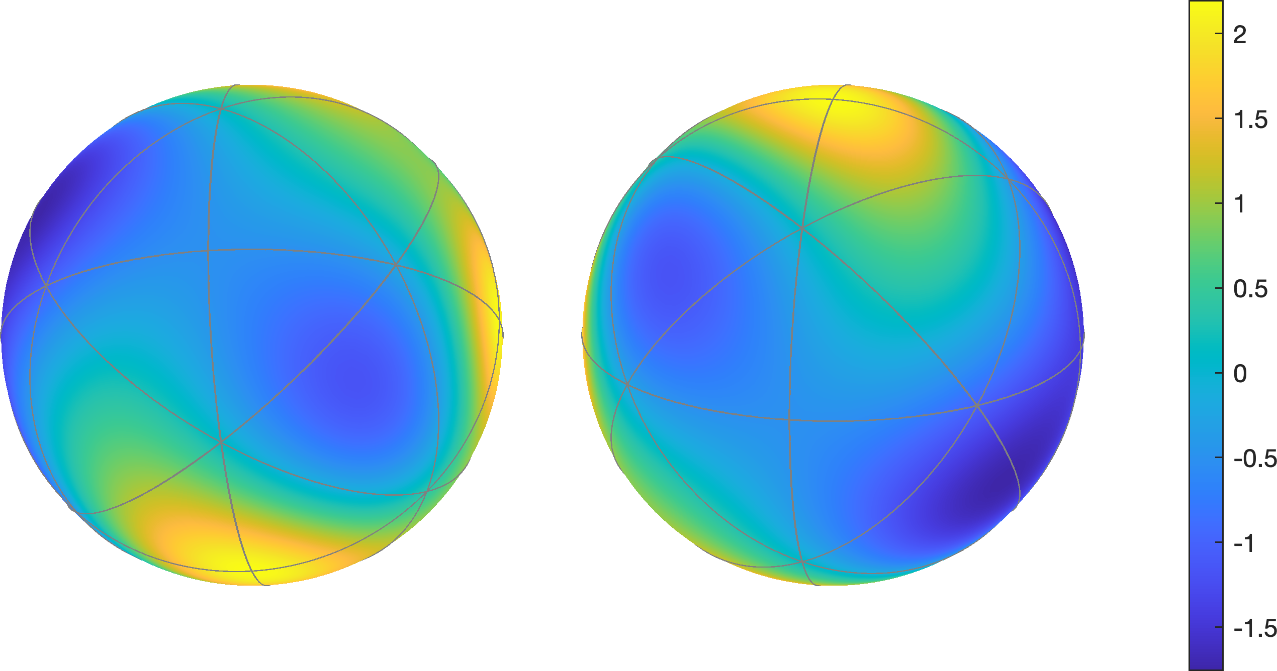
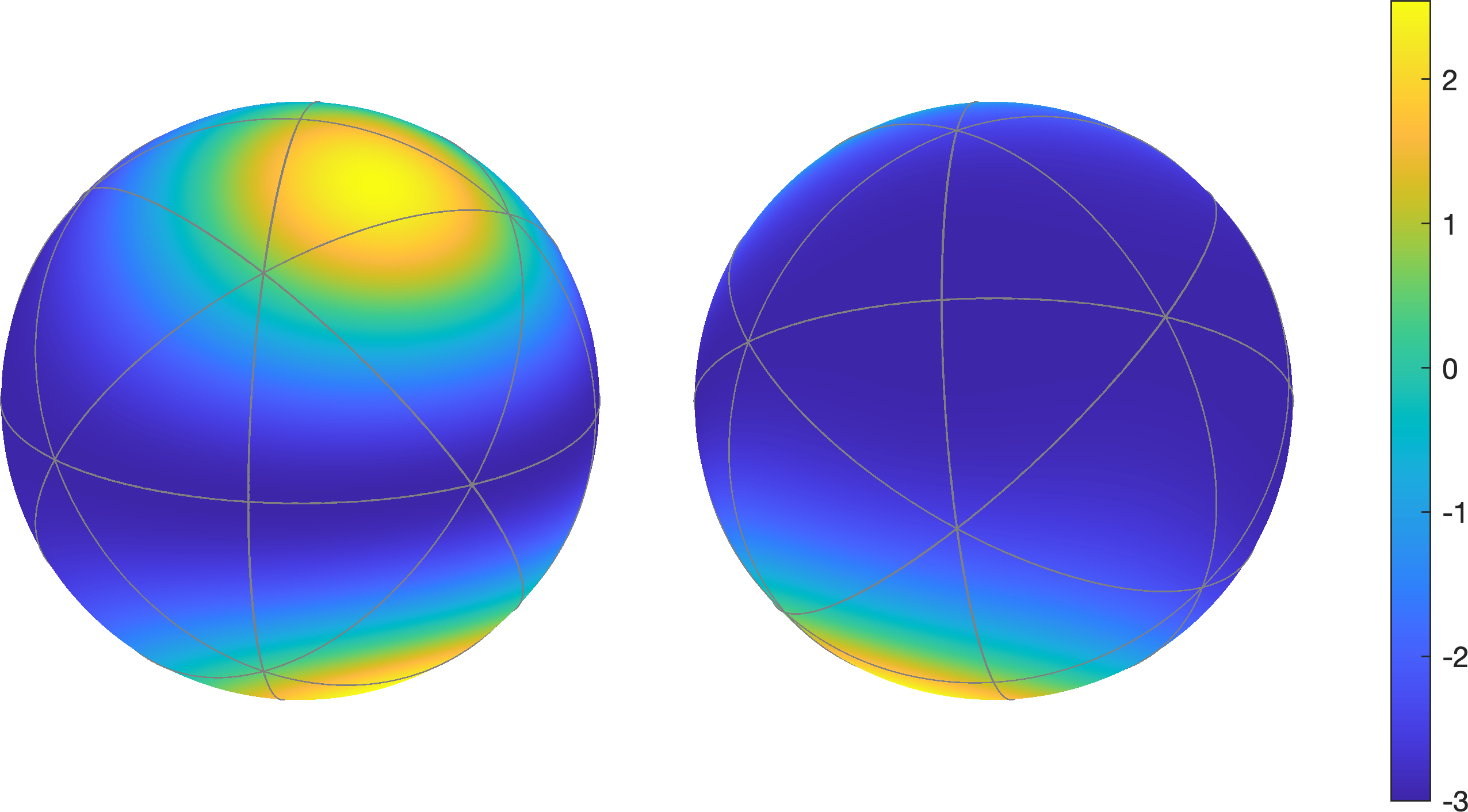
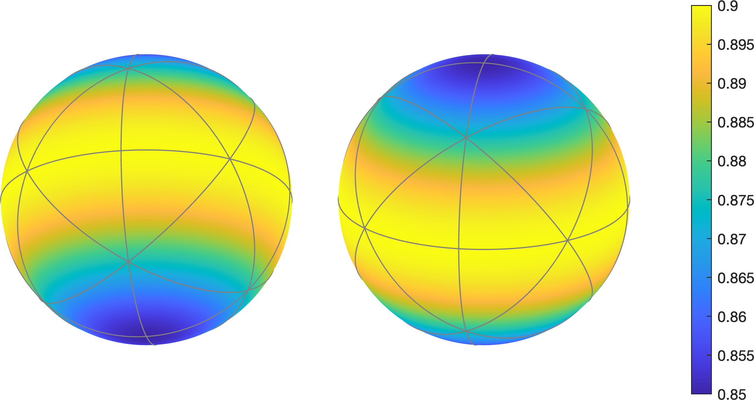
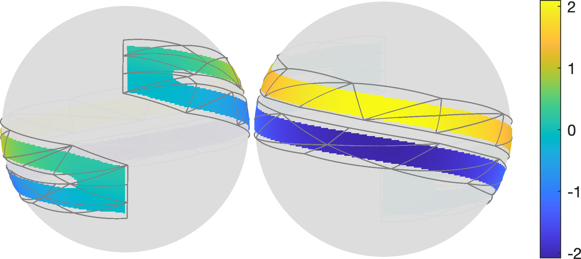
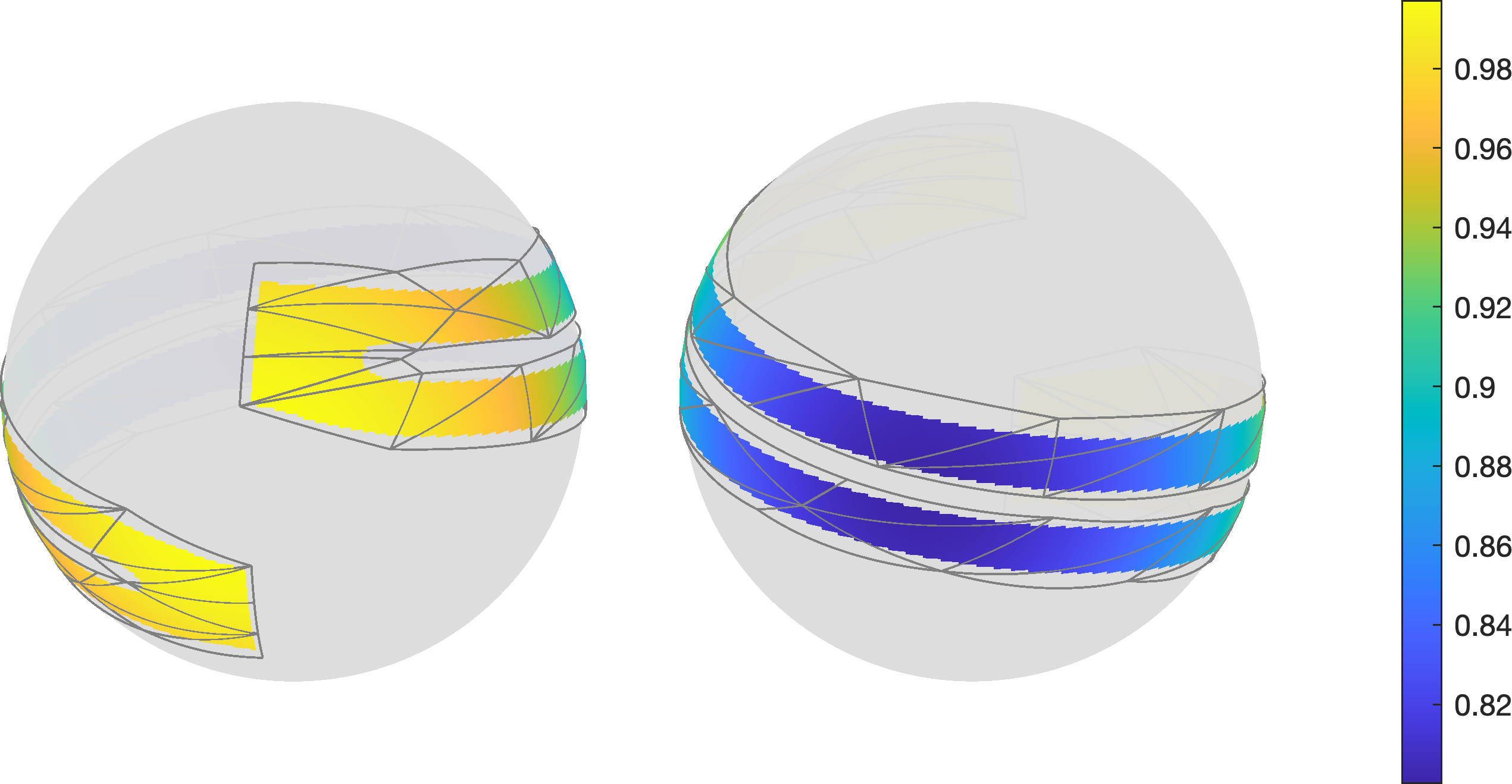
where $m(\mathbf{x}):\mathbb{S}^{2}\to\mathbb{R}$ represents the mean function, and we consider two mean functions: (i) $m_{1}(\mathbf{x})=-2+1/2\{x_{1}^{2}+\exp(2x_{2}^{3})+\exp(2x_{3}^{2})+10x_{1}x_{2}x_{3}\}$; (ii) $m_{2}(\mathbf{x})=2.5\{(x_{1}-1)(x_{2}-1)x_{3}^{2}\}-3$. The illustration of $m_{1}$ and $m_{2}$ is presented in Figure 4 (a) and (b). We generate $\mathbf{X}_{i}$’s on $n=$ 400, 900, and 2,500 grid locations on a unit sphere for training and evaluate the performance of the estimators at $N_{g}=$ 10,201 grid points $\{\mathbf{x}_{j}\}_{j=1}^{N_{g}}$ on the sphere for each simulation setting, which is fixed across all 100 replications. We consider both constant standard deviation $\sigma_{1}(\mathbf{x})\equiv\sigma$ ($\sigma=0.50,~{}0.75$), and heterogeneous standard deviation function $\sigma_{1}(\mathbf{x})$, which varies across different spatial locations. Specifically, we define $\sigma_{1}(\mathbf{x})=c_{\sigma}\{1-(x_{1}^{2}+x_{2}^{2}+1.5x_{3}^{2})/10\}$, where $c_{\sigma}$ takes values of $0.50$ and $0.75$. A visual representation of the standard deviation function $\sigma_{1}(\mathbf{x})$ can be found in Figure 4 (c).

(a) $m_{1}|{\mathbb{S}^{2}}$

(b) $m_{2}|{\mathbb{S}^{2}}$

(c) $\sigma_{1}|\mathbb{S}^{2}$

(d) $m_{3}|{\Omega}$

(e) $\sigma_{2}|\Omega$

Figure 4: Plots of the true mean and standard deviation functions in simulation studies: (a) $m_{1}|{\mathbb{S}^{2}}$ with triangulation ($N=32$) from two viewpoints; (b) $m_{2}|{\mathbb{S}^{2}}$ with triangulation ($N=32$) from two viewpoints; (c) $\sigma_{1}|\mathbb{S}^{2}$ with $c_{\sigma}=1$ from two viewpoints; and (d) $m_{3}|\Omega$ with triangulation ($N=58$); and (e) $\sigma_{2}|\Omega$, with $c_{\sigma}=1$ from two viewpoints.

5.1.1 Comparative analysis of TSSS with competing methods

In this section, we conduct a comparative analysis between the proposed TSSS method and the Kernel and TPSOS methods. To evaluate the performance of different estimators, we use two metrics: the predicted mean squared error (PMSE) and the training mean squared error (TMSE). The PMSE is calculated on a set of grid points $\{\mathbf{x}_{j}\}_{j=1}^{N_{g}}$ on the sphere, and is defined as $N_{g}^{-1}\sum_{j=1}^{N_{g}}\{m(\mathbf{x}_{j})-\widehat{m}(\mathbf{x}_{j})\}^{2}$, where $m$ and $\widehat{m}$ are the true and generic estimated functions. The TMSE is calculated on the training data locations $\{\mathbf{X}_{i}\}_{i=1}^{n}$ and is defined as $n^{-1}\sum_{i=1}^{n}\{m(\mathbf{X}_{i})-\widehat{m}(\mathbf{X}_{i})\}^{2}$. In addition, we report the dimension of the design parameters (“Dim”) and the average computation time per replication (“Time”), measured in seconds.

Due to the similar results, we only report the results in the heterogeneous standard deviation setting in Table 1 and defer the results in the constant standard deviation setting to the Supplementary Material. Table 1 reports the estimation results for $m_{1}|\mathbb{S}^{2}$ and $m_{2}|\mathbb{S}^{2}$ when the errors are heterogeneous with varying standard deviation function: $\sigma_{1}(\mathbf{x})=c_{\sigma}\{1-(x_{1}^{2}+x_{2}^{2}+1.5x_{3}^{2})/10\}$. For TSSS, we utilize the triangulation mesh with $N=32$ triangles, illustrated in Figure 4, along spherical spline basis, which are based on either a fixed degree ($d=3$) or a degree selected via the CV ($d_{\text{CV}}$), as described in Section 4.2.

In Table 1, it is evident that at a lower noise level ($\sigma=0.5$), TSSS with degree $d=3$ outperforms others with the smallest PMSE and TMSE across all sample sizes, suggesting its robustness in precision. For a higher noise level ($\sigma=0.75$), the TSSS with CV-selected degree $d_{\text{CV}}$ consistently exhibits strong performance, often achieving or competing for the lowest errors, which reflects its effective handling of increased variability. Conversely, Tensor-Sphere shows relatively poor performance, with the highest PMSE and TMSE values under both noise conditions, marking it as the least accurate. Kernel and TPSOS generally achieve moderate error rates, neither excelling nor performing the poorest across the different scenarios. These patterns remain consistent as the sample size increases from 400 to 2500, indicating that the relative performance of these methods is stable across different amounts of data.

Regarding computational efficiency, as indicated in Table 1, the Kernel method is the most time-consuming among the methods considered. Comparatively, Tensor-Sphere stands out due to its minimal computational time. The TSSS with a fixed degree $d$ and the TPSOS estimators exhibit similar computational performance. The TSSS with a CV-selected degree $d$ exhibits a slightly slower computational pace, as anticipated, but remains significantly faster, by hundreds or thousands of times, than the Kernel method. Therefore, TSSS achieves a favorable balance between estimation efficacy and computational efficiency for functions defined on the entire sphere.

Table 1: Simulation Study 1 results for different estimation methods on two mean functions $m_{1}|\mathbb{S}^{2}$ and $m_{2}|\mathbb{S}^{2}$ with varying standard deviation function $\sigma_{1}(\mathbf{x})$: the average (and standard deviations) of predicted mean squared error (PMSE), training mean squared error (TMSE), dimension of the design parameters (Dim), and computation time per iteration in seconds (Time). The results for TSSS are based on a triangulation with $N=32$ triangles and spline basis functions with either a fixed degree $d=3$ or a CV-selected degree $d_{\text{CV}}$. TPSOS and Tensor-Sphere have dimensions $k=100$ and $k=64$, respectively. Kernel method results have only $30$ iterations instead of $100$ due to computation inefficiency. A factor of $10^{3}$ scales the reported average (and standard deviations) of PMSEs and TMSEs. Results for $m_{1}|\mathbb{S}^{2}$ and $m_{2}|\mathbb{S}^{2}$ with constant standard deviation function can be found in Table A.2 in Supplementary Material.

$m_{1}|\mathbb{S}^{2}$
		$n=400$						$n=900$						$n=2500$
$c_{\sigma}$	Method	PMSE		TMSE		Dim	Time(s)	PMSE		TMSE		Dim	Time(s)	PMSE		TMSE		Dim	Time(s)
0.5	Kernel	22.61	(4.6)	19.71	(3.9)	400	4901	10.29	(2.1)	9.95	(2.1)	900	8325	5.28	(0.8)	5.17	(0.7)	2500	23207
	TPSOS	25.59	(4.7)	23.11	(4.2)	100	2	13.33	(2.2)	12.72	(2.1)	100	4	6.26	(1.0)	6.12	(0.9)	100	8
	Tensor-Sphere	50.41	(11.4)	38.64	(6.7)	64	0	39.18	(4.5)	33.70	(4.0)	64	0	35.97	(1.9)	32.20	(2.3)	64	0
	TSSS, $d=3$	21.78	(4.5)	19.43	(3.9)	57	3	12.97	(2.0)	12.15	(1.9)	57	3	7.85	(0.9)	7.58	(0.8)	57	3
	TSSS, $d_{\text{CV}}$	23.07	(6.0)	20.44	(4.8)	102	19	11.19	(2.4)	10.58	(2.3)	129	24	4.56	(0.9)	4.48	(0.8)	151	41
0.75	Kernel	47.27	(9.9)	41.51	(8.4)	400	4893	20.04	(4.7)	19.52	(4.6)	900	8252	8.89	(1.8)	8.74	(1.7)	2500	23583
	TPSOS	45.72	(8.9)	42.57	(8.5)	100	2	24.55	(4.4)	23.75	(4.2)	100	3	11.50	(1.9)	11.32	(1.9)	100	8
	Tensor-Sphere	74.20	(13.1)	60.24	(10.0)	64	0	52.10	(6.7)	45.51	(5.7)	64	0	41.24	(2.7)	37.08	(2.9)	64	0
	TSSS, $d=3$	39.82	(9.3)	36.23	(8.1)	57	3	22.72	(4.3)	21.50	(4.1)	57	3	11.94	(2.0)	11.63	(1.9)	57	3
	TSSS, $d_{\text{CV}}$	39.66	(10.4)	36.08	(8.8)	110	19	21.19	(4.8)	20.32	(4.7)	115	23	9.92	(1.9)	9.74	(1.8)	132	41
$m_{2}|\mathbb{S}^{2}$
		$n=400$						$n=900$						$n=2500$
$c_{\sigma}$	Method	PMSE		TMSE		Dim	Time(s)	PMSE		TMSE		Dim	Time(s)	PMSE		TMSE		Dim	Time(s)
0.5	Kernel	21.26	(5.1)	18.72	(4.3)	400	4356	8.60	(2.3)	8.33	(2.3)	900	9771	3.11	(0.8)	3.07	(0.8)	2500	26619
	TPSOS	22.18	(4.7)	20.82	(4.3)	100	9	11.57	(2.4)	11.12	(2.2)	100	19	5.42	(0.9)	5.29	(0.9)	100	39
	Tensor-Sphere	25.68	(6.9)	19.94	(4.5)	64	0	12.81	(3.4)	10.40	(2.3)	64	0	5.48	(1.0)	4.72	(0.8)	64	0
	TSSS, $d=3$	16.73	(4.2)	15.37	(3.7)	57	3	8.61	(2.0)	8.27	(1.9)	57	3	3.59	(0.9)	3.55	(0.9)	57	4
	TSSS, $d_{\text{CV}}$	18.19	(5.6)	16.69	(4.9)	86	21	8.91	(2.1)	8.57	(2.0)	71	29	3.42	(0.9)	3.39	(0.8)	60	49
0.75	Kernel	46.94	(10.9)	41.54	(9.3)	400	4355	19.30	(5.3)	18.70	(5.3)	900	9763	6.99	(1.9)	6.90	(1.8)	2500	26642
	TPSOS	40.41	(9.4)	38.67	(8.8)	100	8	21.39	(4.7)	20.74	(4.5)	100	18	9.94	(1.8)	9.76	(1.8)	100	40
	Tensor-Sphere	47.97	(12.6)	38.93	(9.1)	64	0	24.51	(6.4)	20.41	(4.7)	64	0	10.42	(2.1)	9.04	(1.8)	64	0
	TSSS, $d=3$	36.40	(9.3)	33.58	(8.2)	57	3	19.04	(4.5)	18.30	(4.3)	57	3	7.96	(2.0)	7.88	(2.0)	57	4
	TSSS, $d_{\text{CV}}$	34.77	(10.1)	32.51	(8.9)	80	21	16.47	(4.7)	15.92	(4.5)	64	28	6.76	(1.8)	6.71	(1.8)	61	48

5.1.2 Impact of $d$ and $\triangle$, and CV for $d$ and $\lambda$ on TSSS Estimation

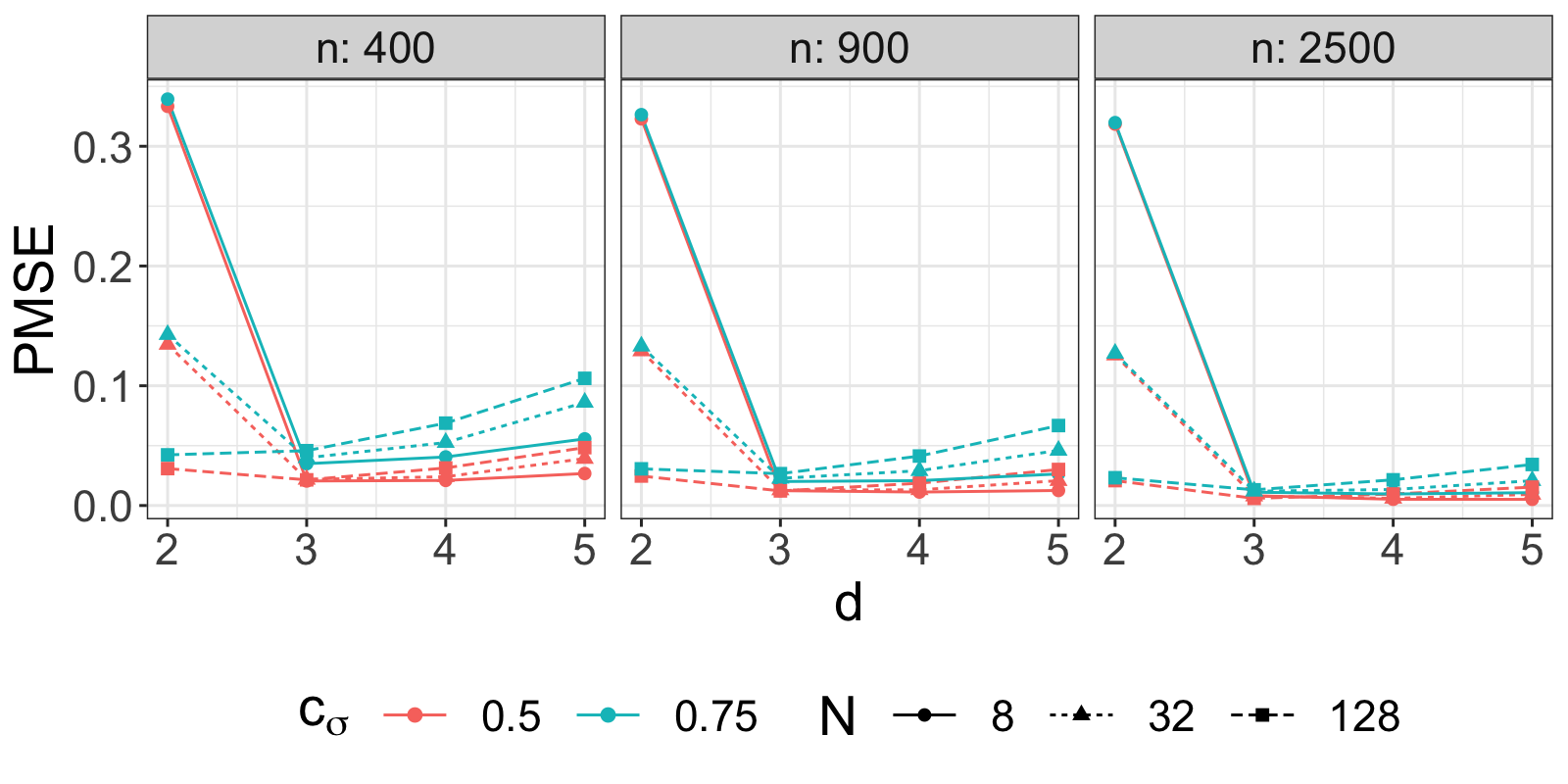
This section investigates the effect of degree $d$ and triangulation $\triangle$ on the estimation performance for the TSSS method. We also investigate the behavior of CV-selected $d$ and $\lambda$, and their impact on the TSSS estimation. Specifically, we first investigate the impact of $d$ and $\triangle$ on TSSS methods under different $\sigma$ and $n$ settings. In addition, we fix $\triangle$ and select the optimal combination of $d$ and penalty parameter $\lambda$ through the CV method and study the behavior of CV-selected $d_{\text{CV}}$ compared to fixed $d$’s.

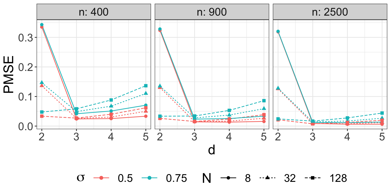
The results in Figure 5 reveal that different combinations of $d$ and triangulation can lead to varied TSSS performance. Firstly, when $d$ is small, a finer triangulation improves PMSE; see $d=2$. In contrast, for larger $d$, a finer triangulation may not necessarily improve the PMSE, as observed in the cases of $d=3,4,5$. This is because a larger degree $d$ and number of triangles $N$ can lead to over-parameterization of the mean function. Secondly, when $d$ is too small for a fixed triangulation, the mean functions may not be fully represented, leading to underfitting. Thirdly, as the sample size $n$ increases, both $d$ and the fineness of triangulation may need to be adjusted to achieve optimal estimation performance. When the noise is small, the estimated mean function can better approximate the true mean function, which allows for a higher degree of spline basis $d$ and a finer triangulation to be used without overfitting. However, the choice of $d$ and $N$ should still be balanced with computational efficiency, as both a very high $d$ and a very large $N$ can lead to high computational costs. In general, a careful trade-off between accuracy and computational efficiency must be considered when choosing the appropriate $d$ and $N$ for a given sample size and noise level. Readers are referred to Section 4 for a detailed discussion.

(a) $m_{1}|{\mathbb{S}^{2}}$

(b) $m_{2}|{\mathbb{S}^{2}}$

(c) $m_{1}|\mathbb{S}^{2}$

(d) $m_{2}|\mathbb{S}^{2}$

Figure 5: (a) & (b): Performance of TSSS for $m_{1}|\mathbb{S}^{2}$ and $m_{2}|\mathbb{S}^{2}$ in Simulation Study 1 with different $n$, $d$, $c_{\sigma}$, and $N$. Additional results based on the constant standard deviation setting can be found in Figure A.1 in Supplementary Material; (c) & (d) Bar graphs of $d_{\text{CV}}$ under different combinations of $c_{\sigma}=0.50,~{}0.75$ (sig), $n=400,~{}900,~{}2,500$, and $N=8,~{}32,~{}128$ in Simulation Study 1. Results of the constant standard deviation setting can be found in Figure A.2 of Supplementary Material.

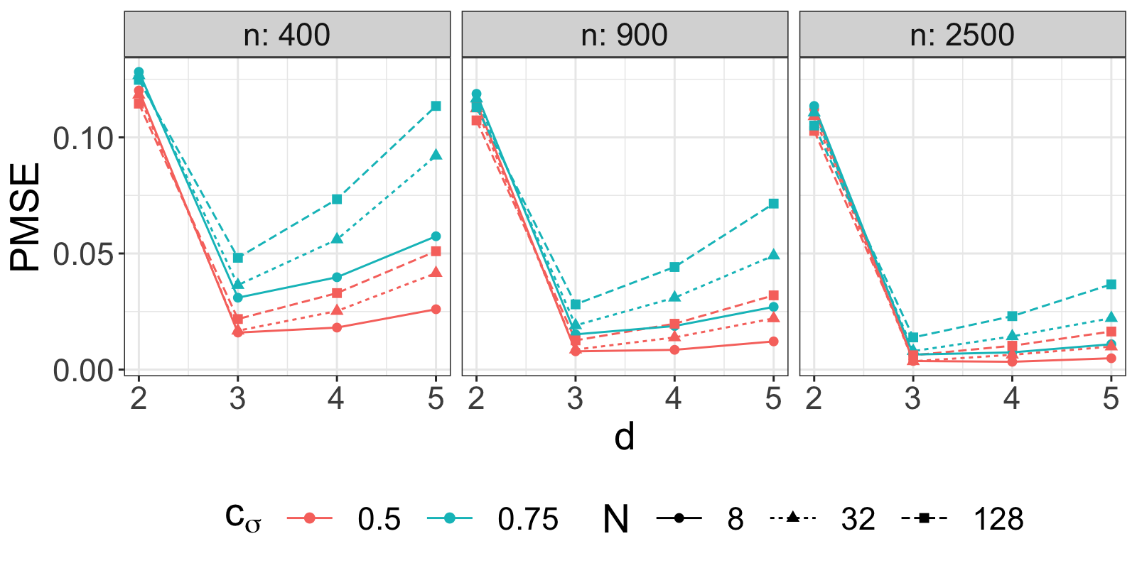
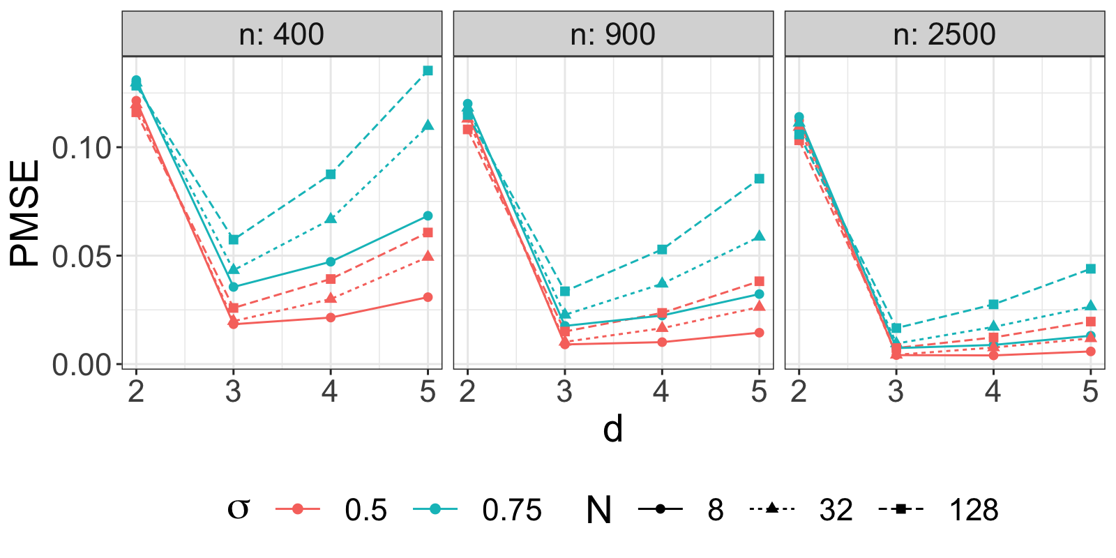
Next, we assess the performance of the TSSS estimator employing spline basis functions with the selected degree $d_{\text{CV}}$. As before, we consider simulation settings with various combinations of parameters: $n=400,~{}900,~{}2500$; $d=2,~{}3,~{}4,~{}5$; $c_{\sigma}=0.50,~{}0.75$; and $N=8,~{}32,~{}128$, applied to $m_{1}|\mathbb{S}^{2}$ and $m_{2}|\mathbb{S}^{2}$. For each setting, we simulate $\{(\mathbf{X}_{i},Y_{i})\}_{i=1}^{n}$ and compute the TSSS estimator using the selected $d_{\text{CV}}$. This procedure is repeated $100$ times for each setting. The bar graphs in Figure 5 and columns “$f_{d_{\text{CV}}}$” in Table 2 illustrate the empirical frequency of $d_{\text{CV}}$ across various settings. Table 2 also presents the PMSE of TSSS estimators for $d=2,~{}3,~{}4,~{}5$ and $d_{\text{CV}}$. From the table and bar graphs, for fixed $n,~{}\sigma$, as $N$ increases, smaller $d_{\text{CV}}$’s are selected. This is consistent with our previous discussion about the balance between $d$ and $N$. In addition, when $n$ and $N$ are fixed, as $\sigma$ increases, a smaller $d_{\text{CV}}$ tends to be selected. This trend is reasonable because higher $d$ tends to pick up more noise, which does not benefit the overall fitting. Furthermore, compared to TSSS estimators with fixed $d=2,~{}3,~{}4,~{}5$, the TSSS estimator with $d_{\text{CV}}$ is among the best in terms of PMSEs. Therefore, the proposed procedure of selecting $d$ and $\lambda$ by CV is validated.

Table 2: Performance comparison of TSSS Estimators for $m_{1}|\mathbb{S}^{2}$ and $m_{2}|\mathbb{S}^{2}$ in Simulation Study 1: $d_{\text{CV}}$ vs. fixed degree $d=2,~{}3,~{}4,~{}5$. The frequency of selecting $d_{\text{CV}}$ among $100$ replications is denoted as $f_{d_{\text{CV}}}$. The reported average (and standard deviations) of PMSEs are scaled by a factor of $10^{3}$. Additional results for $m_{1}|\mathbb{S}^{2}$ and $m_{2}|\mathbb{S}^{2}$ based on the constant standard deviation function setting can be found in Table A.3 in Supplementary Material.

$m_{1}|\mathbb{S}^{2}$
		$N=8$						$N=32$						$N=128$
		$n=400$		$n=900$		$n=2500$		$n=400$		$n=900$		$n=2500$		$n=400$		$n=900$		$n=2500$
$c_{\sigma}$	$d$	PMSE	$f_{d_{\text{CV}}}$	PMSE	$f_{d_{\text{CV}}}$	PMSE	$f_{d_{\text{CV}}}$	PMSE	$f_{d_{\text{CV}}}$	PMSE	$f_{d_{\text{CV}}}$	PMSE	$f_{d_{\text{CV}}}$	PMSE	$f_{d_{\text{CV}}}$	PMSE	$f_{d_{\text{CV}}}$	PMSE	$f_{d_{\text{CV}}}$
0.5	2	333.35	0	322.90	0	318.50	0	134.50	0	129.03	0	125.59	0	30.84	20	24.63	0	20.80	0
		(7.82)		(2.73)		(1.29)		(4.93)		(2.21)		(0.88)		(4.45)		(1.55)		(0.66)
	3	20.48	55	12.43	30	8.20	0	21.78	54	12.97	24	7.85	1	21.44	65	12.21	90	5.96	99
		(3.78)		(1.81)		(0.60)		(4.48)		(1.99)		(0.89)		(4.33)		(1.99)		(0.93)
	4	20.95	39	11.24	63	5.21	62	24.05	45	13.11	76	6.01	99	31.36	11	18.62	10	9.62	1
		(5.50)		(2.18)		(0.93)		(5.18)		(2.15)		(0.94)		(5.37)		(2.31)		(1.13)
	5	26.74	6	12.57	7	5.15	38	39.22	1	20.74	0	9.28	0	48.33	4	30.09	0	15.37	0
		(5.59)		(2.31)		(0.95)		(7.09)		(2.91)		(1.28)		(7.18)		(3.23)		(1.52)
	$d_{\text{CV}}$	21.79	–	12.04	–	5.29	–	23.07	–	11.19	–	4.56	–	23.95	–	11.34	–	4.79	–
		(4.95)		(2.36)		(0.96)		(6.02)		(2.44)		(0.85)		(5.83)		(2.16)		(0.89)
0.75	2	339.35	0	326.40	0	319.74	0	142.69	0	133.00	0	127.03	0	42.30	46	30.63	10	23.20	0
		(9.91)		(4.08)		(1.72)		(8.59)		(3.82)		(1.44)		(8.87)		(3.19)		(1.29)
	3	34.93	74	20.03	56	11.10	22	39.82	44	22.72	40	11.94	21	45.79	35	26.61	87	13.11	100
		(7.84)		(3.72)		(1.29)		(9.25)		(4.32)		(2.04)		(9.54)		(4.45)		(2.06)
	4	40.56	23	20.79	41	9.63	70	52.58	56	29.05	59	13.39	79	68.78	17	41.31	3	21.46	0
		(11.16)		(4.75)		(1.95)		(11.34)		(4.80)		(2.10)		(11.94)		(5.18)		(2.55)
	5	55.64	3	26.37	3	10.76	8	86.11	0	46.00	1	20.72	0	106.21	2	66.79	0	34.26	0
		(12.20)		(4.90)		(2.08)		(15.65)		(6.46)		(2.87)		(16.06)		(7.26)		(3.41)
	$d_{\text{CV}}$	36.85	–	20.78	–	10.12	–	39.66	–	21.19	–	9.92	–	41.01	–	20.26	–	8.99	–
		(9.13)		(4.19)		(1.94)		(10.42)		(4.76)		(1.90)		(10.56)		(5.06)		(1.66)
$m_{2}|\mathbb{S}^{2}$
		$N=8$						$N=32$						$N=128$
		$n=400$		$n=900$		$n=2500$		$n=400$		$n=900$		$n=2500$		$n=400$		$n=900$		$n=2500$
$c_{\sigma}$	$d$	PMSE	$f_{d_{\text{CV}}}$	PMSE	$f_{d_{\text{CV}}}$	PMSE	$f_{d_{\text{CV}}}$	PMSE	$f_{d_{\text{CV}}}$	PMSE	$f_{d_{\text{CV}}}$	PMSE	$f_{d_{\text{CV}}}$	PMSE	$f_{d_{\text{CV}}}$	PMSE	$f_{d_{\text{CV}}}$	PMSE	$f_{d_{\text{CV}}}$
0.5	2	120.16	0	115.00	0	112.18	0	118.35	0	112.43	0	109.05	0	114.51	0	107.31	0	102.80	0
		(3.87)		(1.91)		(0.86)		(4.72)		(2.10)		(0.92)		(5.25)		(2.26)		(1.04)
	3	15.94	70	7.86	55	3.70	26	16.73	71	8.61	85	3.59	96	21.77	63	12.59	100	6.19	99
		(4.27)		(1.89)		(0.62)		(4.19)		(2.02)		(0.91)		(4.51)		(2.25)		(0.99)
	4	18.09	28	8.52	43	3.37	74	25.22	28	13.85	15	6.39	4	32.94	35	19.75	0	10.27	1
		(5.51)		(2.12)		(0.83)		(5.37)		(2.35)		(1.01)		(5.70)		(2.64)		(1.23)
	5	25.98	2	12.14	2	4.89	0	41.55	1	22.04	0	9.92	0	50.97	2	31.96	0	16.39	0
		(5.52)		(2.35)		(0.99)		(7.75)		(3.10)		(1.38)		(7.79)		(3.65)		(1.65)
	$d_{\text{CV}}$	17.01	–	8.43	–	3.47	–	18.19	–	8.91	–	3.42	–	18.83	–	8.64	–	4.03	–
		(4.80)		(2.31)		(0.84)		(5.62)		(2.07)		(0.86)		(5.14)		(2.03)		(0.79)
0.75	2	128.22	0	118.76	0	113.52	0	126.73	0	116.68	0	110.67	0	124.75	0	112.93	0	105.09	0
		(8.28)		(3.51)		(1.49)		(8.64)		(3.67)		(1.58)		(9.64)		(4.02)		(1.77)
	3	30.97	72	15.18	67	6.48	58	36.40	77	19.04	92	7.96	95	48.14	94	28.09	100	13.86	100
		(9.17)		(3.99)		(1.34)		(9.27)		(4.46)		(2.04)		(10.13)		(5.00)		(2.22)
	4	39.77	24	18.76	33	7.41	42	56.02	22	30.96	8	14.31	5	73.37	6	44.18	0	23.00	0
		(12.39)		(4.70)		(1.91)		(11.99)		(5.25)		(2.28)		(12.85)		(5.89)		(2.77)
	5	57.41	4	27.01	0	10.92	0	92.09	1	49.10	0	22.17	0	113.51	0	71.49	0	36.71	0
		(12.36)		(5.26)		(2.22)		(17.14)		(6.95)		(3.10)		(17.50)		(8.16)		(3.71)
	$d_{\text{CV}}$	34.18	–	16.17	–	6.69	–	34.77	–	16.47	–	6.76	–	32.07	–	17.43	–	8.60	–
		(10.06)		(4.61)		(1.62)		(10.12)		(4.71)		(1.80)		(8.26)		(4.13)		(1.70)

5.2 Simulation Study 2: Functions on Irregularly Shaped Spherical Patches

In this simulation study, we generate the response variable $Y_{i}$ from the following model:

$$Y_{i}=m_{3}(\mathbf{X}_{i})+\sigma_{2}(\mathbf{X}_{i})\epsilon_{i},~{}\epsilon_{i}\overset{i.i.d}{\sim}N(0,1),~{}i=1,\ldots,n,$$ (9)

with mean function $m_{3}:\Omega\to\mathbb{R}$ and varying standard deviation function $\sigma_{2}(\mathbf{x})=1-(1.5(x_{1}+1)^{2}+x_{2}^{2}+x_{3}^{2})/30$ defined on irregularly shaped spherical patch $\Omega$. Specifically, for $\mathbf{x}\in\Omega$, we define $m_{3}(\mathbf{x})=\widetilde{m}_{3}(\mathbf{x}^{\prime})$, where $\widetilde{m}_{3}(\mathbf{x})=(0.08\pi+0.84+x_{1})I(x_{1}\geq-0.84,x_{3}>0)-(0.08\pi+0.84+x_{1})I(x_{1}\geq-0.84,x_{3}\leq 0)-0.16\arctan\{x_{3}/(0.84+x_{1})\}I(x_{1}<-0.84)$; the spherical coordinates of $\mathbf{x}$, $(\theta,\phi)$, and the spherical coordinates of $\mathbf{x}^{\prime}$, $(\theta^{\prime},\phi^{\prime})$, satisfy $\theta^{\prime}=\theta,~{}\phi^{\prime}=\phi+\theta/6$. This choice of $m_{3}$ allows us to test the performance of the methods for functions with complex patterns on non-standard spherical domains. See Figure 4 for a visualization of the mean function and standard deviation function. We generate $\mathbf{X}_{i}$’s on $n=400,~{}900$ and $2,500$ random locations on the complex domains for training. The SNRs of Simulation Study 2 are reported in Table A.1.

For TSSS, given that $m_{3}$ is not wildly oscillating, we select a spline basis based on $d=2$ and a triangulation mesh with $56$ triangles. The triangulation is constructed by mapping the spherical domain to the planar domain, triangulating the planar domain using TriMesh from R package “Triangulation” (Wang and Lai, 2019), and mapping the planar triangulation back to spherical coordinates. This procedure would require the user to provide boundary points and interior holes’ boundary points and adjust the identical boundary points that wrap around the longitude or co-latitude. This practice is suitable and recommended for simple domains due to the nice properties of TriMesh function. Refer to Figure 4 (d) for the triangulation.

Then, we calculate the PMSE by evaluating the performance on $11,986$ grid points for $m_{3}|\Omega$. The estimation results are shown in Table 3. The table shows that TSSS, both with a fixed degree ($d=2$) and a cross-validation-selected degree ($d_{\text{CV}}$), outperforms TPSOS, Kernel and Tensor-Sphere in terms of both PMSE and TMSE across all settings. In addition to its superior estimation accuracy, TSSS demonstrates significant computational benefits over the Kernel approach. It achieves a reasonable computation efficiency that is comparable to TPSOS, especially for larger sample sizes. Although the Tensor-Sphere method frequently records minimal computational times, at times as low as zero seconds, it falls short of TSSS in terms of estimation accuracy. The success of TSSS is attributed to its ability to address the “leakage” problem by adopting “domain-aware” splines. This simulation study highlights the advantages of TSSS in addressing complex domain issues and the “leakage” problem, while maintaining computational efficiency.

Table 3: Simulation Study 2 results for different estimation methods on mean function $m_{3}|\Omega$ with varying standard deviation function $\sigma_{2}(\mathbf{x})$: the average (and standard deviations) of predicted mean squared error (PMSE), training mean squared error (TMSE), dimension of the design parameters (Dim), and computation time per iteration in seconds (Time). TSSS settings: $d=2$ or a CV-selected $d_{\text{CV}}$, $N=58$, $r=1$. TPSOS and Tensor-Sphere have dimensions $k=100$ and $k=64$, respectively. Kernel method results have only $30$ iterations instead of $100$ due to computation inefficiency. A factor of $10^{3}$ scales the reported average (and standard deviations) of PMSEs and TMSEs. Additional results for mean functions $m_{3}|\Omega$ with constant standard deviation function can be found in Table A.4 in Supplementary Material.

$m_{3}|\Omega$
		$n=400$						$n=900$						$n=2500$
$c_{\sigma}$	Method	PMSE		TMSE		Dim	Time(s)	PMSE		TMSE		Dim	Time(s)	PMSE		TMSE		Dim	Time(s)
0.5	Kernel	141.48	(31.6)	132.00	(33.7)	400	1928	108.22	(44.3)	107.12	(45.5)	900	4978	51.16	(7.0)	52.35	(7.2)	2500	21692
	TPSOS	95.68	(12.8)	64.73	(7.0)	100	10	53.36	(5.3)	44.31	(4.2)	100	20	31.64	(1.5)	31.16	(1.7)	100	43
	Tensor-Sphere	58.26	(7.0)	51.14	(5.6)	64	0	42.73	(4.0)	40.03	(4.8)	64	0	30.01	(1.5)	30.64	(1.6)	64	0
	TSSS, $d=2$	17.69	(5.3)	16.02	(4.4)	45	25	9.72	(2.5)	9.08	(2.1)	45	25	4.94	(0.8)	4.81	(0.8)	45	25
	TSSS, $d_{\text{CV}}$	18.08	(6.0)	16.25	(4.3)	100	263	9.88	(2.2)	9.30	(2.1)	85	325	4.69	(0.9)	4.53	(0.9)	132	270
0.75	Kernel	167.81	(13.7)	157.96	(18.6)	400	1928	133.84	(35.4)	132.22	(35.3)	900	4948	82.62	(41.6)	84.45	(43.3)	2500	21301
	TPSOS	139.64	(17.0)	107.79	(12.8)	100	10	78.65	(8.6)	68.12	(7.7)	100	21	41.77	(2.9)	41.15	(2.8)	100	44
	Tensor-Sphere	79.56	(12.9)	71.57	(10.3)	64	0	55.80	(5.3)	54.42	(5.5)	64	0	36.30	(3.1)	37.01	(3.1)	64	0
	TSSS, $d=2$	32.27	(10.8)	29.72	(9.2)	45	25	17.17	(4.7)	16.30	(4.4)	45	25	8.24	(1.8)	8.03	(1.8)	45	25
	TSSS, $d_{\text{CV}}$	30.42	(9.3)	28.39	(8.0)	54	341	17.62	(5.4)	16.75	(4.9)	63	333	8.66	(1.9)	8.46	(1.8)	68	359

5.3 Simulation Study 3: Stability of TSSS Estimator

In this simulation study, we verify the stability of the TSSS estimator through a bootstrap procedure. We conduct a total of $200$ Monte Carlo (MC) replications. In each replication, we simulate observations $\{(\mathbf{X}_{i},Y_{i})\}_{i=1}^{n}$, using the same data generation settings as those employed in Simulation Study 2 in Section 5.2. For simplicity, we fix $\mathbf{X}_{i}$’s on a grid with $n=3,065$, $d=3$, and $c_{\sigma}=0.5$.

Then, the bootstrap standard errors (SE) of TSSS estimator are generated through Algorithm 1 using $B=100$ wild bootstrap samples, denoted as $\{\text{SE}_{R}^{\text{Boot}}\}_{R=1}^{{200}}$. We report the mean and median of $\{\text{SE}_{R}^{\text{Boot}}\}_{R=1}^{{200}}$, denoted them as $\text{SE}^{\text{Boot}}_{\text{mean}}$ and $\text{SE}^{\text{Boot}}_{\text{median}}$, respectively. The Monte Carlo standard error $\text{SE}^{\text{MC}}$ from ${{200}}$ TSSS estimators are calculated from the MC replications, and serves as the ground truth. We then compare $\text{SE}^{\text{MC}}$ to $\text{SE}^{\text{Boot}}_{\text{mean}}$ and $\text{SE}^{\text{Boot}}_{\text{median}}$ in Figure 6. The similarity between the Bootstrap SE estimator and the Monte Carlo SE estimator demonstrates the stability of the TSSS estimator.

Figure 6: Standard error function plots for $m_{3}|\Omega$ in Simulation Study 3: from left to right, $\text{SE}^{\text{MC}}$, $\text{SE}^{\text{Boot}}_{\text{mean}}$, and $\text{SE}^{\text{Boot}}_{\text{median}}$.

6 Data Applications

6.1 Cortical Surface fMRI Data

In our first application, we apply the proposed TSSS method to estimate the mean neural activity of the brain using the Human Connectome Project (HCP) data (Van Essen et al., 2013). The HCP is a comprehensive data project that maps macroscopic human brain circuits and their relationship to human behavior. Specifically, we use the cs-fMRI data from the Motor task study of the HCP 500-subject data release. In this study, participants are asked to tap their left or right fingers, squeeze their left or right foot, or move their tongue following visual cues. During the experiment, two runs of task fMRI scans were collected. One run was collected by scanning the brain from left to right (LR), and the other run was from right to left (RL) (Woolrich et al., 2001).

In this study, we use the RL scan run of a randomly sampled subject (Subject #100307) registered to the low-resolution Conte 69 standard mesh, which contains approximately $32,000$ vertices per hemisphere (Glasser et al., 2013; Van Essen et al., 2012; Jenkinson et al., 2012; Fischl, 2012; Van Essen et al., 2012). In addition, to evaluate the performance of TSSS in both the resting and task states, the first frame at the subject’s resting state ($t=0$s) and the 20th frame after left-hand tapping is onset ($t\approx 15$s) are studied. For each frame, we perform a 10-fold CV procedure to examine the prediction accuracy. For visualization, we map the predicted values from the sphere to the mid-thickness brain surface, using R package “ciftiTools” (Pham et al., 2022).

For the TSSS method, the triangulation is constructed by first obtaining a uniform triangulation of the whole sphere. Next, we select only the spherical triangles containing observations and adjust the boundary points to obtain a smoother domain shape. This step can be more complex, as it requires careful consideration of the underlying data distribution and geometry of the domain. However, in our experience, the triangulation works well even without the adjustment step as long as there are no triangles containing extremely sparse observations. Two settings are studied for TSSS: (i) $r=1,~{}d=5$ with a modest fine triangulation $N=473$, as shown in Figure 7; and (ii) $r=1,~{}d=3$ with a fine triangulation $N=1,913$ for each hemisphere.

(a)

(b)

Figure 7: Triangulation for (a) Human Right Hemisphere from two viewpoints ($N=473$); and (b) the ocean surface from two viewpoints ($N=380$).

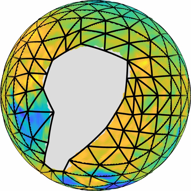
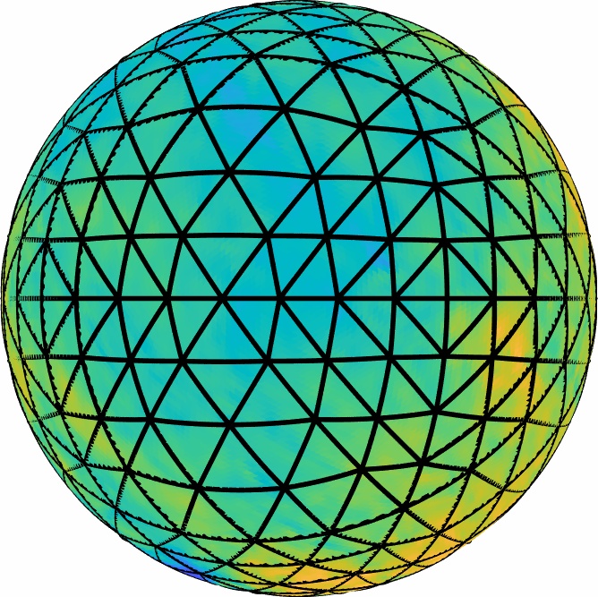
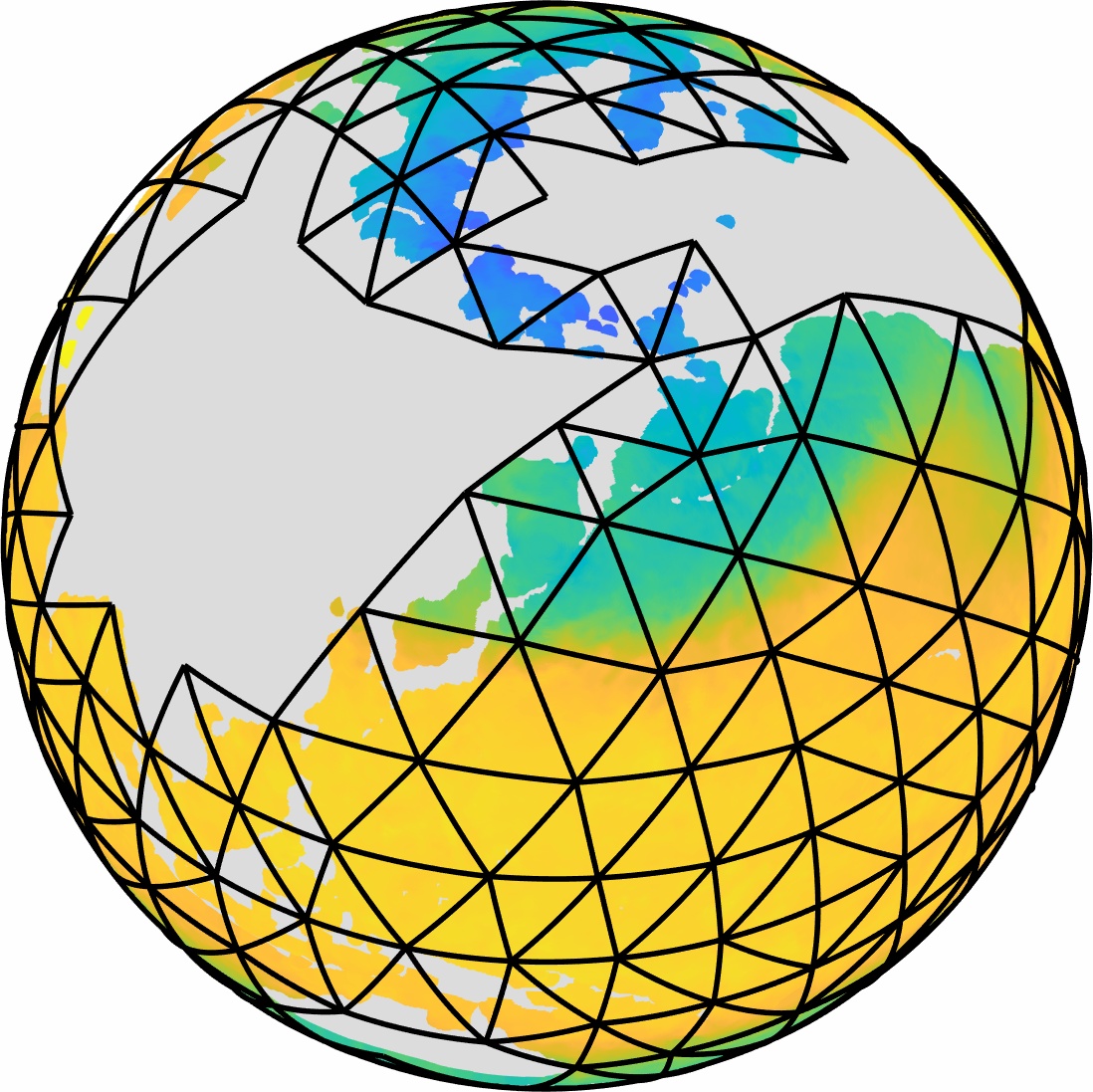
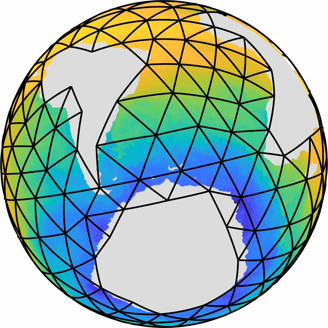
Table 4 reports the mean and standard deviation of the cross-validated root mean squared prediction error (CV-RMSPE), $[N_{k}^{-1}\sum_{i:k[i]=k}\{Y_{i}-\widehat{m}^{-k}(\mathbf{X}_{i})\}^{2}]^{-1/2},\,k=1,\ldots,10$, for TSSS, TPSOS and Tensor-Sphere, where the Kernel method is omitted due to its computation inefficiency. Here $k[i]$ is the index of the fold that contains the $i$-th observation, $N_{k}$ is the cardinality of the $k$-th fold, and $\widehat{m}^{-k}$ is the fitted mean function using data excluding the $k$-th fold. From Table 4, we observe that when the dimensions of TPSOS, TSSS and Tensor-Sphere are similar, around $2,000$, TSSS demonstrates a slight advantage over TPSOS and a more significant advantage compared to Tensor-Sphere. However, as the dimension of TPSOS increases to around $2,900$, the advantage of TSSS over both TPSOS and Tensor-Sphere becomes more pronounced. These results hold consistently for both hemispheres and different brain activity periods. Importantly, TSSS offers researchers greater flexibility in achieving their objectives. Depending on the desired outcome, researchers can adjust the parameters accordingly. Higher values of $d$ and $N$ can be employed to recover detailed signals, while finer triangulation can be used to incorporate prior domain knowledge. Moreover, by tuning the smoothness coefficient $r$, researchers can control the level of smoothness in the estimated function, aligning it with their expectations. TSSS thus provides a versatile tool for researchers with diverse needs and preferences.

Table 4: The mean (and standard deviation) of CV-RMSPE in the HCP data application based on TPSOS, Tensor-Sphere and TSSS. The number of parameters for TPSOS and Tensor-Sphere are set to be $2,000$ and $2,025$, respectively. The settings for TSSS are as follows: (i) $r=1,~{}d=5,~{}N=473$, yielding a dimensionality (Dim) of $2,921$; and (ii) $r=1,~{}d=3,~{}N=1,913$, yielding a dimensionality (Dim) of approximately $2,000$.

Left Hemisphere				Right Hemisphere
Frame	Method	CV-RMSPE	Dim	Frame	Method	CV-RMSPE	Dim
1	TPSOS	471 (26)	2000	1	TPSOS	421 (11)	2000
1	Tensor-Sphere	528 (26)	2025	1	Tensor-Sphere	468 (15)	2025
1	TSSS (i)	412 (11)	2921	1	TSSS (i)	370   (8)	2921
1	TSSS (ii)	460 (15)	2003	1	TSSS (ii)	409 (10)	2008
20	TPSOS	467 (26)	2000	20	TPSOS	415 (12)	2000
20	Tensor-Sphere	527 (29)	2025	20	Tensor-Sphere	463 (14)	2025
20	TSSS (i)	407 (12)	2921	20	TSSS (i)	365   (9)	2921
20	TSSS (ii)	457 (16)	2003	20	TSSS (ii)	411 (10)	2008

Furthermore, we employ the bootstrap method outlined in Algorithm 1 to estimate the standard error of the TSSS estimator. To facilitate better visualization, we present the standard error normalized by the maximum observed value, denoted as $\text{SE}^{\text{Boot}}/\max_{i}\{Y_{i}\}$. In Figure 8, we provide visual representations of the observed, predicted, and residual values for the first frame of both hemispheres using TSSS with setting (ii). The estimated standard errors are consistently small across the whole domain.

(a) HCP

(b) Temp

(c) Humid

Figure 8: (a) The observed, predicted, residual values along with the estimated standard error of the TSSS estimator for the first frame in HCP data application. Rows 1 and 2 depict two different viewpoints for each hemisphere. The TSSS settings used are: $r=1,~{}d=3$, and $N=1,913$; (b) & (c): The observed, predicted, and residual values along with the estimated standard error of the TSSS estimator for Temp and Humid in oceanic atmospheric data application. The TSSS settings used are: $d=3$, $r=1$, and $N=1,513$.

6.2 Oceanic Atmospheric Data

In this application, we apply our method to the NOAA Ocean Surface Bundle Climate Data Record (CDR) from the National Centers for Environmental Information (NCEI) (Clayson et al., 2016). In particular, we consider the dataset SEAFLUX-OSB-CDR_V02R00_ATMOS_D20210831_C20211223.nc and focus on the specific humidity (Humid) and air temperature (Temp) on August 31, 2021. There are approximately one million lattice locations on the surface of Earth, among which approximately 485,000 locations are observed.

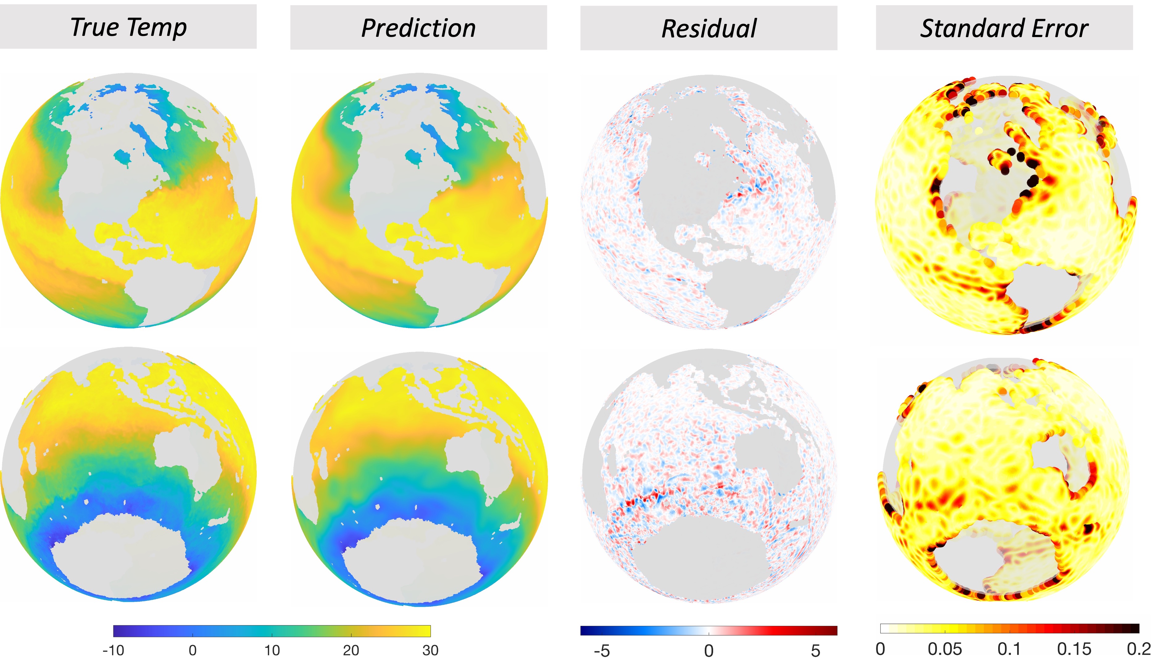
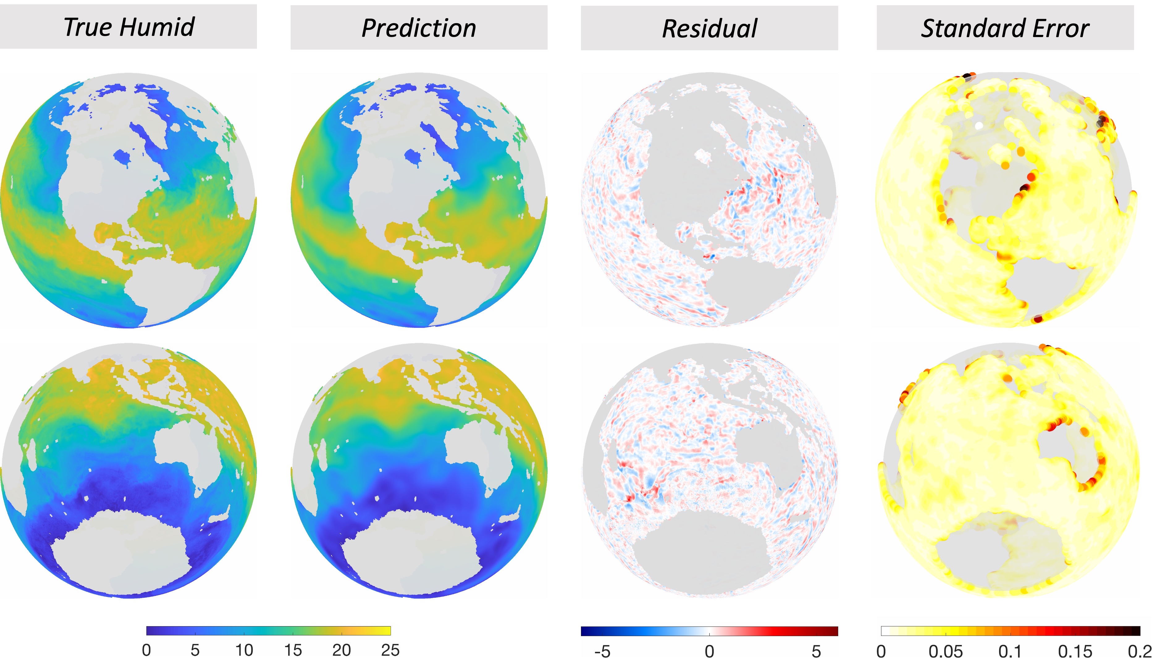
Again, we apply a 10-fold CV procedure to evaluate the performance of TSSS, TPSOS, and Tensor-Sphere. For TSSS, we use settings (i) $d=5$, $r=1$ with a modest fine triangulation $N=380$, as shown in Figure 7; and (ii) $d=3$, $r=1$ with a fine triangulation $N=1,513$ for the ocean surface. The triangulation is constructed in the same way as described in Section 6.1. The results in Table 5 indicate that TSSS outperforms Tensor-Sphere under both settings. At the same time, TSSS with setting (i) outperforms TPSOS but is inferior to TPSOS under setting (ii). Therefore, the results show that TSSS outperforms TPSOS in terms of prediction accuracy when appropriate triangulation and tuning parameters are selected, while the advantage of TSSS over Tensor-Sphere remains consistent. Figure 8 displays the observed, predicted values, residuals of humidity and temperature, along with the estimated standard error of TSSS with setting (ii). The residuals do not exhibit patterns, and the estimated standard errors are satisfyingly small, with slightly larger values along the boundary of domains. This is reasonable since fewer observations are available near the domain boundary.

Table 5: The mean (and standard deviation) of the CV-RMSPEs in NCEI data application based on TSSS and TPSOS. The settings for TPSOS and Tensor-Sphere are $2,000$ and $2,025$, respectively. The TSSS settings used are: (i) $r=1,~{}d=5,~{}N=380$, yielding a dimensionality (Dim) of $2,600$; and (ii) $r=1,~{}d=3,~{}N=1,513$, yielding a dimensionality (Dim) of $1,947$.

Item	Methods	CV-RMSPE	Dim	Item	Methods	CV-RMSPE	Dim
Temp	TPSOS	0.4913 (0.004)	2000	Humid	TPSOS	0.3808 (0.004)	2000
	Tensor-Sphere	0.5667 (0.008)	2025		Tensor-Sphere	0.4992 (0.011)	2025
	TSSS (i)	0.4684 (0.003)	2600		TSSS (i)	0.3522 (0.001)	2600
	TSSS (ii)	0.5171 (0.003)	1947		TSSS (ii)	0.3925 (0.001)	1947

7 Summary and Discussion

Motivated by ubiquitous surface-based data in various fields, we introduce a novel TSSS estimator for data that resides on complex domains on the sphere or any surface that can be properly mapped to and back from the sphere. The combination of penalized spline methods and triangulation techniques on spherical surfaces or patches presents a novel methodology makes TSSS advantageous in handling complex spherical domains while enjoying enhanced computation efficiency.

Firstly, TSSS provides enhanced flexibility in capturing complex spatial patterns, allowing for accurate modeling of intricate variations in the data. By employing the “domain aware” splines, TSSS enables estimation to enjoy accuracy without suffering from “leakage” or boundary effects. This distinguishes TSSS from its competitors (e.g., Tensor-Sphere, TPSOS, and kernel-based methods). Secondly, TSSS offers improved computational efficiency compared to the kernel-based approach, making it more scalable for large-scale datasets. Kernel-based approaches use observed locations as the centers of kernels. However, such kernel functions do not necessarily constitute the most efficient basis for approximating highly localized or rapidly changing functions. On the contrary, TSSS constructs basis functions based on triangulated domains and avoids the need for excessive basis functions. By adaptively refining the triangulation and utilizing spline basis functions with a flexible degree and smoothness, TSSS can better capture the complexity of the underlying signal. Thirdly, we provide rigorous theoretical guarantees and an implementation algorithm for the uncertainty quantification of TSSS. Specifically, Theorem 2 demonstrates the asymptotic normality of the TSSS estimator, and Algorithm 1 introduces a wild Bootstrap algorithm to obtain the standard error map of the TSSS estimator. These advantages have all been demonstrated through extensive numerical experiments.

The studies in this paper also open up opportunities for further research. Note that TSSS usually requires well-constructed triangulations that accurately approximate the shape of domains. When the domain contains isolated sub-domains, determining whether to connect these sub-domains in the triangulation can be challenging and may require human input. To overcome this challenge, researchers could develop automated triangulation procedures to construct triangulations that work well with the TSSS method, where users’ desired configuration could be easily tuned. Moreover, inspired by Basna et al. (2022), there is potential to explore function-dependent triangulation methods under functional data settings. In particular, random samples of functional data can be used to customize triangulations using data-specific features.

Another interesting future research direction is to advance TSSS to accommodate datasets that possess physical constraints, such as non-negativity (Baramidze and Lai, 2018; Kim et al., 2021; Zhang et al., 2022a) and shape constraints (Wang et al., 2020b; Fang et al., 2022). Incorporating non-negativity constraints into the TSSS framework can broaden the method’s applicability to datasets where negative values are physically infeasible or meaningless. Moreover, integrating constraints (e.g., monotonicity, convexity, symmetry, or specific geometric patterns) into the TSSS framework can provide additional regularization to ensure the estimated function adheres to predefined physical constraints. TSSS can also be extended to handle longitudinal or time series data observed on spherical domains. Allowing researchers to model the dynamics of surface-based data over time could offer essential insights, such as estimating the temporal change of Earth’s atmospheric properties. Furthermore, in functional data regression where surface-based imaging serves as functional responses or covariates (Lila and Aston, 2020), TSSS can be used as the first smoothing step.

It is also of immense interest to extend the proposed TSSS method to the hypersphere setting. Data that lies on the surface of hyperspheres is commonly referred to as “directional data”. It is widely observed during the investigation of cell cycle data (Schafer, 1998); the shape analysis of manifold-valued data (Lin et al., 2017); compositional household expenditure (Scealy and Welsh, 2017); and gene expression clustering (Ding and Regev, 2021). Within this body of literary works, the hypersphere-valued data $\mathbf{x}\in\mathbb{S}^{d}$ are regarded as the response of interest, and their traits carry information. Although our framework focuses more on the estimation of mean function with $\mathbf{x}\in\mathbb{S}^{d}$ being the covariates, we can utilize dimension reduction methods proposed in the directional data literature to counter the high-dimension setting in our framework.

In particular, it is possible to project data that lies on a hypersphere onto an optimal sphere using the method proposed by Luo et al. (2022), followed by the TSSS procedure. Specifically, if $\mathbf{x}\in\Omega\subseteq\mathbb{S}^{d}$, the geometric distance can be utilized to find the best lower dimension representation of the given domain $\Omega$ in $\mathbb{S}^{d^{\prime}}$. When the targeting dimension $d^{\prime}=2$, we can get the dataset’s best unit sphere projection. The estimation of the mean function with hypersphere support can then be treated as one with unit sphere support. Then, the proposed TSSS method can be directly used without the triangulation of hypersphere domains, which can be easily infeasible when $d$ is very large.

In addition to the location variable $\mathbf{x}$, datasets frequently incorporate explanatory variables $\{z_{k},k=1,\ldots,p\}$, which may also contribute to the model. To account for that, we can utilize the generalized additive mean structure introduced in Yu et al. (2020b), $g\{\mu(\mathbf{z},\mathbf{x})\}=\sum_{k=1}^{p}f_{k}(z_{k})+m(\mathbf{x})$. Here $g$ can be any link function, and $m(\cdot),f_{k}(\cdot)$ can be estimated nonparametrically depending on the assumption of the function space of $m(\cdot),f_{k}(\cdot)$. Another potential approach is the generalized spatially varying coefficient models (Kim and Wang, 2021). These modeling frameworks offer researchers the opportunity to explore the relationship between local features and responses of interest that reside on a surface.

Appendix A Numerical Results

In this section, we provide supplementary results for simulation studies considering homogeneous random errors with a constant standard deviation.

Table A.1: Signal-to-noise ratios (SNRs) for simulation studies.

Simulation Study 1								Simulation Studies 2 & 3
Constant standard deviation				Varying standard deviation				Constant standard deviation		Varying standard deviation
$m_{1}|\mathbb{S}^{2}$		$m_{2}|\mathbb{S}^{2}$		$m_{1}|\mathbb{S}^{2}$		$m_{2}|\mathbb{S}^{2}$		$m_{3}|\Omega$		$m_{3}|\Omega$
$\sigma$	SNR	$\sigma$	SNR	$c_{\sigma}$	SNR	$c_{\sigma}$	SNR	$\sigma$	SNR	$c_{\sigma}$	SNR
0.50	5.14	0.50	4.78	0.50	6.72	0.50	6.25	0.50	7.83	0.50	7.81
0.75	2.28	0.75	2.13	0.75	2.98	0.75	2.78	0.75	3.48	0.75	3.47

Table A.2: Simulation Study 1 results for different estimation methods on two mean functions $m_{1}|\mathbb{S}^{2}$ and $m_{2}|\mathbb{S}^{2}$ with homogeneous errors: the average (and standard deviations) of predicted mean squared error (PMSE), training mean squared error (TMSE), dimension of the design parameters (Dim), and computation time per iteration in seconds (Time). A factor of $10^{3}$ scales the reported average (and standard deviations) of PMSEs and TMSEs. The results for TSSS are based on a triangulation with $N=32$ triangles and spline basis functions with either a fixed degree $d=3$ or a CV-selected degree $d_{\text{CV}}$. The results for TPSOS and Tensor-Sphere are based on dimensions $k=100$ and $k=64$, respectively. Kernel method results have only $30$ iterations instead of $100$ due to computation inefficiency.

$m_{1}|\mathbb{S}^{2}$
		$n=400$						$n=900$						$n=2500$
$\sigma$	Method	PMSE		TMSE		Dim	Time(s)	PMSE		TMSE		Dim	Time(s)	PMSE		TMSE		Dim	Time(s)
0.5	Kernel	28.27	(5.8)	24.71	(4.9)	400	6036	12.52	(2.7)	12.15	(2.7)	900	3532	6.11	(1.0)	6.00	(1.0)	2500	11085
	TPSOS	30.80	(5.7)	28.04	(5.2)	100	2	16.20	(2.8)	15.51	(2.6)	100	4	7.59	(1.2)	7.43	(1.2)	100	8
	Tensor-Sphere	57.18	(13.1)	44.45	(7.4)	64	0	42.70	(5.1)	36.82	(4.4)	64	0	37.38	(2.1)	33.48	(2.4)	64	0
	TSSS, $d=3$	25.91	(5.6)	23.30	(4.9)	57	3	15.17	(2.5)	14.27	(2.4)	57	3	8.82	(1.2)	8.53	(1.1)	57	3
	TSSS, $d_{\text{CV}}$	27.06	(7.0)	24.20	(5.8)	101	20	13.36	(2.9)	12.68	(2.7)	126	27	5.71	(1.0)	5.61	(1.0)	150	48
0.75	Kernel	59.84	(12.5)	52.65	(10.6)	400	6040	25.04	(6.0)	24.43	(5.9)	900	3521	10.75	(2.3)	10.59	(2.1)	2500	11030
	TPSOS	54.96	(11.0)	51.44	(10.6)	100	1	29.77	(5.5)	28.87	(5.3)	100	4	13.98	(2.4)	13.76	(2.3)	100	8
	Tensor-Sphere	86.75	(15.6)	71.32	(12.1)	64	0	58.83	(8.1)	51.60	(6.8)	64	0	44.07	(3.2)	39.66	(3.2)	64	0
	TSSS, $d=3$	49.01	(11.4)	44.82	(10.2)	57	3	27.61	(5.2)	26.22	(5.0)	57	3	14.03	(2.5)	13.71	(2.4)	57	3
	TSSS, $d_{\text{CV}}$	48.61	(12.9)	44.52	(10.8)	110	20	26.35	(5.8)	25.33	(5.7)	108	26	12.68	(2.4)	12.46	(2.4)	109	46
$m_{2}|\mathbb{S}^{2}$
		$n=400$						$n=900$						$n=2500$
$\sigma$	Method	PMSE		TMSE		Dim	Time(s)	PMSE		TMSE		Dim	Time(s)	PMSE		TMSE		Dim	Time(s)
0.5	Kernel	25.44	(5.9)	22.52	(5.1)	400	1452	10.27	(2.7)	9.96	(2.7)	900	3339	3.74	(1.0)	3.70	(1.0)	2500	9820
	TPSOS	25.25	(5.4)	23.86	(4.9)	100	2	13.25	(2.7)	12.77	(2.5)	100	4	6.19	(1.1)	6.06	(1.0)	100	7
	Tensor-Sphere	28.96	(7.6)	22.79	(5.1)	64	0	14.60	(3.9)	11.92	(2.6)	64	0	6.24	(1.2)	5.38	(0.9)	64	0
	TSSS, $d=3$	19.79	(4.9)	18.26	(4.3)	57	3	10.24	(2.3)	9.85	(2.2)	57	3	4.27	(1.1)	4.23	(1.1)	57	4
	TSSS, $d_{\text{CV}}$	21.33	(6.1)	19.69	(5.2)	87	23	10.36	(2.3)	9.99	(2.3)	73	29	3.90	(1.0)	3.87	(1.0)	60	44
0.75	Kernel	55.88	(12.4)	49.76	(10.9)	400	1449	23.03	(6.1)	22.33	(6.0)	900	3312	8.40	(2.2)	8.32	(2.1)	2500	9820
	TPSOS	45.92	(10.6)	44.20	(10.0)	100	2	24.45	(5.3)	23.77	(5.0)	100	4	11.37	(2.1)	11.19	(2.1)	100	8
	Tensor-Sphere	53.91	(14.0)	44.27	(10.3)	64	0	27.94	(7.7)	23.37	(5.6)	64	0	11.89	(2.4)	10.35	(2.0)	64	0
	TSSS, $d=3$	43.27	(10.9)	40.10	(9.6)	57	3	22.72	(5.2)	21.86	(5.0)	57	3	9.47	(2.4)	9.39	(2.3)	57	4
	TSSS, $d_{\text{CV}}$	39.20	(11.9)	37.06	(10.7)	75	23	19.01	(5.5)	18.42	(5.3)	63	28	7.79	(1.9)	7.75	(1.9)	58	44

Table A.3: Performance comparison of TSSS Estimators for $m_{1}|\mathbb{S}^{2}$ and $m_{2}|\mathbb{S}^{2}$ in Simulation Study 1: $d_{\text{CV}}$ vs. fixed degree $d=2,~{}3,~{}4,~{}5$, in the setting of homogeneous standard error with constant standard deviation $\sigma$. The frequency of selecting $d_{\text{CV}}$ among $100$ replications is denoted as $f_{d_{\text{CV}}}$. The reported average (and standard deviations) of PMSEs are scaled by a factor of $10^{3}$.

$m_{1}|\mathbb{S}^{2}$
		$N=8$						$N=32$						$N=128$
		$n=400$		$n=900$		$n=2500$		$n=400$		$n=900$		$n=2500$		$n=400$		$n=900$		$n=2500$
$\sigma$	d	PMSE	$f_{d_{\text{CV}}}$	PMSE	$f_{d_{\text{CV}}}$	PMSE	$f_{d_{\text{CV}}}$	PMSE	$f_{d_{\text{CV}}}$	PMSE	$f_{d_{\text{CV}}}$	PMSE	$f_{d_{\text{CV}}}$	PMSE	$f_{d_{\text{CV}}}$	PMSE	$f_{d_{\text{CV}}}$	PMSE	$f_{d_{\text{CV}}}$
0.5	2	335.03	0	323.74	0	318.80	0	136.40	0	129.96	0	125.93	0	33.49	30	26.08	0	21.38	0
		(8.35)		(3.04)		(1.38)		(5.78)		(2.59)		(1.02)		(5.45)		(1.91)		(0.81)
	3	24.11	65	14.26	38	8.87	1	25.91	55	15.17	27	8.82	2	27.04	48	15.52	93	7.60	99
		(4.67)		(2.27)		(0.78)		(5.56)		(2.50)		(1.16)		(5.52)		(2.56)		(1.19)
	4	25.32	30	13.42	55	6.34	75	30.59	44	16.76	73	7.69	98	39.99	18	23.84	7	12.34	1
		(6.79)		(2.72)		(1.15)		(6.57)		(2.75)		(1.21)		(6.87)		(2.96)		(1.46)
	5	33.35	5	15.69	7	6.43	24	49.89	1	26.48	0	11.88	0	61.78	4	38.59	0	19.71	0
		(7.13)		(2.86)		(1.23)		(8.98)		(3.70)		(1.65)		(9.22)		(4.15)		(1.96)
	$d_{\text{CV}}$	25.81	–	14.43	–	6.51	–	27.06	–	13.36	–	5.71	–	29.75	–	13.15	–	5.78	–
		(5.96)		(2.73)		(1.17)		(7.00)		(2.92)		(1.03)		(7.08)		(2.72)		(1.10)
0.75	2	342.96	0	328.20	0	320.39	0	146.63	0	135.05	0	127.77	0	47.57	53	33.40	21	24.36	0
		(11.36)		(4.83)		(1.96)		(10.33)		(4.62)		(1.73)		(10.95)		(3.96)		(1.62)
	3	41.67	75	23.52	62	12.54	34	49.01	44	27.61	47	14.03	45	58.42	33	34.05	79	16.80	100
		(10.31)		(4.59)		(1.65)		(11.43)		(5.15)		(2.54)		(12.22)		(5.72)		(2.65)
	4	50.99	22	25.46	36	11.62	60	67.30	56	37.25	52	17.18	55	88.21	12	53.07	0	27.59	0
		(14.28)		(5.51)		(2.47)		(14.45)		(6.15)		(2.71)		(15.32)		(6.68)		(3.29)
	5	70.56	3	33.59	2	13.63	6	110.15	0	58.91	1	26.56	0	136.45	2	85.91	0	44.04	0
		(15.16)		(6.30)		(2.66)		(19.88)		(8.25)		(3.70)		(20.66)		(9.34)		(4.40)
	$d_{\text{CV}}$	44.03	–	24.56	–	12.13	–	48.61	–	26.35	–	12.68	–	47.37	–	25.14	–	11.21	–
		(11.70)		(5.24)		(2.35)		(12.88)		(5.76)		(2.45)		(13.40)		(6.03)		(2.10)
$m_{2}|\mathbb{S}^{2}$
0.5	2	121.44	0	115.64	0	112.39	0	119.71	0	113.11	0	109.30	0	116.10	0	108.21	0	103.17	0
		(4.37)		(2.17)		(0.95)		(5.38)		(2.38)		(1.01)		(5.92)		(2.53)		(1.14)
	3	18.38	67	9.06	58	4.14	33	19.79	70	10.24	83	4.27	96	25.88	69	15.02	100	7.40	99
		(4.97)		(2.22)		(0.70)		(4.88)		(2.34)		(1.07)		(5.32)		(2.61)		(1.17)
	4	21.45	31	10.13	40	4.00	67	29.97	29	16.54	17	7.64	4	39.22	29	23.60	0	12.28	1
		(6.42)		(2.47)		(0.98)		(6.27)		(2.75)		(1.20)		(6.68)		(3.06)		(1.46)
	5	30.86	2	14.48	2	5.84	0	49.37	1	26.30	0	11.86	0	60.68	2	38.19	0	19.61	0
		(6.48)		(2.74)		(1.16)		(8.99)		(3.65)		(1.64)		(9.14)		(4.25)		(1.95)
	$d_{\text{CV}}$	19.86	–	9.70	–	4.00	–	21.33	–	10.36	–	3.90	–	21.08	–	10.01	–	4.75	–
		(5.68)		(2.71)		(0.95)		(6.08)		(2.33)		(0.99)		(5.81)		(2.29)		(0.92)
0.75	2	130.96	0	120.07	0	113.98	0	129.74	0	118.19	0	111.22	0	128.35	0	114.90	0	105.88	0
		(9.55)		(4.15)		(1.69)		(9.99)		(4.30)		(1.79)		(11.15)		(4.67)		(1.99)
	3	35.57	75	17.61	68	7.38	65	43.27	82	22.72	93	9.47	98	57.39	95	33.58	100	16.59	100
		(10.45)		(4.65)		(1.53)		(10.87)		(5.20)		(2.36)		(11.96)		(5.83)		(2.62)
	4	47.20	22	22.39	32	8.84	35	66.73	17	37.01	7	17.13	2	87.50	5	52.85	0	27.54	0
		(14.18)		(5.50)		(2.23)		(14.03)		(6.16)		(2.71)		(15.07)		(6.83)		(3.28)
	5	68.39	3	32.28	0	13.07	0	109.72	1	58.67	0	26.54	0	135.34	0	85.50	0	43.94	0
		(14.57)		(6.13)		(2.62)		(19.92)		(8.17)		(3.68)		(20.57)		(9.51)		(4.39)
	$d_{\text{CV}}$	38.50	–	19.01	–	7.69	–	39.20	–	19.01	–	7.79	–	37.04	–	20.51	–	10.21	–
		(10.79)		(5.35)		(1.81)		(11.94)		(5.52)		(1.90)		(9.50)		(4.74)		(1.98)

(a)

(b)

Figure A.1: Performance of TSSS for $m_{1}|\mathbb{S}^{2}$ and $m_{2}|\mathbb{S}^{2}$ in Simulation Study 1 in the setting of constant standard deviation with different $n$, $d$, $\sigma$, and $N$.

(a)

(b)

Figure A.2: The bar graphs of $d_{\text{CV}}$ in Simulation Study 1 with homogeneous errors under different combinations of $\sigma=0.50,~{}0.75$ (sig), $n=400,~{}900,~{}2,500$, and $N=8,~{}32,~{}128$.

Table A.4: Simulation Study 2 results for different estimation methods of $m_{3}|\Omega$ with homogeneous errors: the average (and standard deviations) of predicted mean squared error (PMSE), training mean squared error (TMSE), dimension of the design parameters (Dim), and computation time per iteration in seconds (Time). A factor of $10^{3}$ scales the reported average (and standard deviations) of PMSEs and TMSEs. The results for TSSS are based on a triangulation with $N=32$ triangles and spline basis functions with either a fixed degree $d=2$ or a CV-selected degree $d_{\text{CV}}$. The results for TPSOS and Tensor-Sphere are based on dimensions $k=100$ and $k=64$, respectively. Kernel method results have only $30$ iterations instead of $100$ due to computation inefficiency.

$m_{3}|\Omega$
		$n=400$						$n=900$						$n=2500$
$\sigma$	Method	PMSE		TMSE		Dim	Time(s)	PMSE		TMSE		Dim	Time(s)	PMSE		TMSE		Dim	Time(s)
0.5	Kernel	144.14	(30.8)	134.83	(33.5)	400	5882	115.38	(43.1)	114.25	(43.6)	900	9273	54.83	(17.9)	56.34	(19.3)	2500	26355
	TPSOS	103.94	(13.7)	72.71	(8.1)	100	11	57.79	(6.0)	48.50	(4.7)	100	19	33.37	(1.7)	32.88	(1.8)	100	44
	Tensor-Sphere	61.78	(8.1)	54.50	(6.4)	64	0	45.89	(3.7)	43.59	(4.4)	64	0	31.14	(1.8)	31.74	(1.7)	64	0
	TSSS, $d=2$	19.78	(5.9)	18.12	(5.0)	45	25	10.71	(2.5)	10.16	(2.3)	45	25	5.44	(0.9)	5.31	(0.9)	45	26
	TSSS, $d_{\text{CV}}$	20.65	(6.7)	18.78	(5.0)	90	110	11.26	(2.6)	10.65	(2.4)	82	130	5.35	(1.0)	5.21	(1.0)	115	159
0.75	Kernel	173.34	(17.8)	163.18	(24.9)	400	5925	141.53	(31.9)	140.02	(32.6)	900	9271	94.02	(45.1)	96.41	(47.3)	2500	26394
	TPSOS	152.72	(18.3)	121.42	(14.9)	100	11	87.23	(9.8)	76.34	(8.8)	100	21	45.45	(3.4)	44.82	(3.3)	100	42
	Tensor-Sphere	86.48	(15.0)	78.23	(12.2)	64	0	59.44	(6.1)	58.18	(6.3)	64	0	40.05	(3.9)	40.84	(4.3)	64	0
	TSSS, $d=2$	37.37	(12.4)	34.57	(10.6)	45	25	19.77	(5.6)	18.85	(5.3)	45	25	9.27	(2.1)	9.06	(2.0)	45	26
	TSSS, $d_{\text{CV}}$	34.28	(10.3)	32.20	(9.1)	54	121	20.00	(6.2)	19.09	(5.7)	63	138	9.61	(2.1)	9.42	(2.0)	60	173

Appendix B Technical Proofs

B.1. Radial Projection

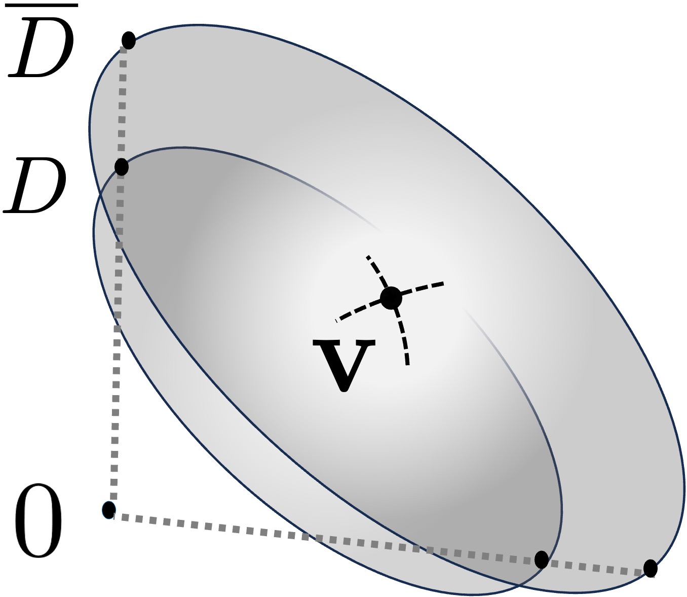
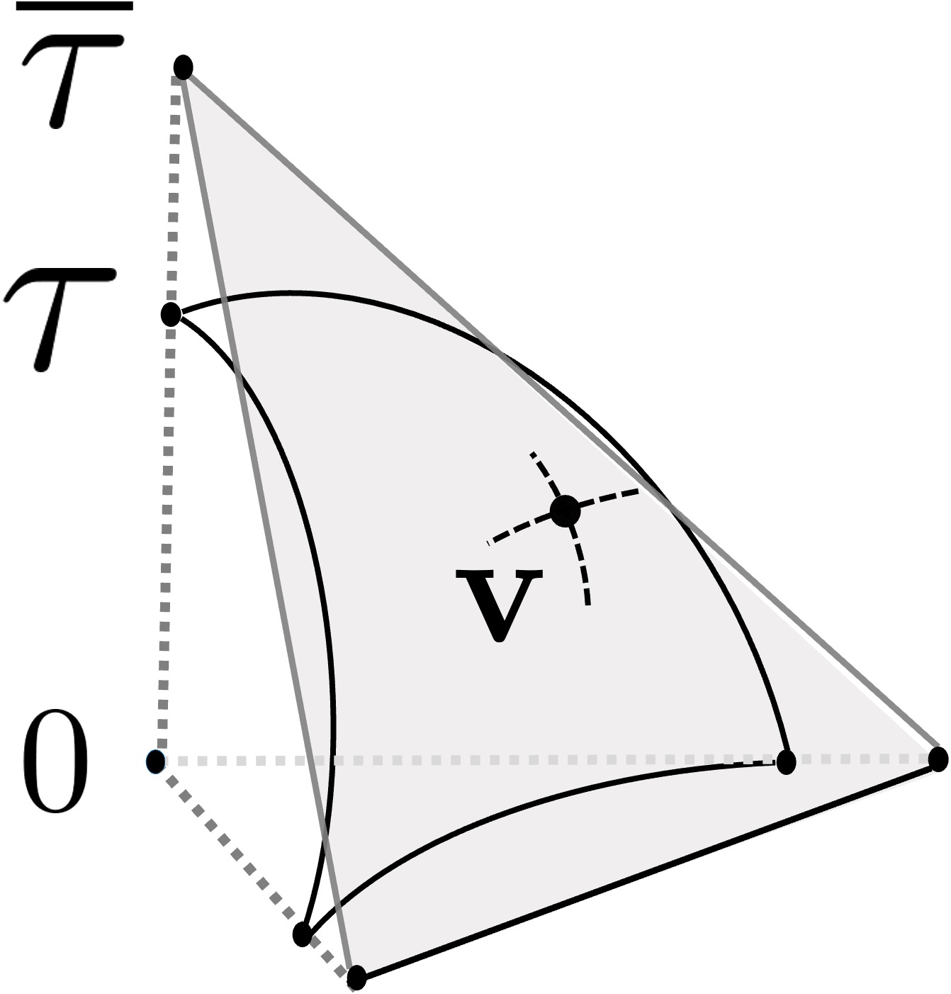
To prepare for the definition of norms on a sphere, we introduce some elements of radial projection, which maps a local spherical domain to a planar 2D domain. Define the radial projection of any point $\mathbf{v}$ in a spherical cap $D$ to a unique point $\overline{\mathbf{v}}$ on the plane $\overline{D}$ tangent to the sphere at $\mathbf{v}_{D}$ through a mapping $\mathcal{R}_{D}:D\to\overline{D}$. Similarly, we can define the projection of a spherical triangle $\tau$ to $\overline{\tau}=\mathcal{R}_{D}\tau$; see illustrations of radial projection in Figure B.1.

(a)	(b)	(c)	(d)

Figure B.1: Illustrations of (a) radial projection of spherical cap $D$, (b) radial projection of spherical triangle $\tau$, (c) tetrahedron $\uptau$, and (d) tetrahedron $\uptau_{1}$.

Remark B.0.

If $\Omega$ is contained in a spherical cap of radius $1/2$, we have the $K_{1}\|f\|_{L^{q}(\Omega)}\leq\|\overline{f}_{p}\|_{L^{q}(\overline{\Omega})}\leq K_{2}\|f\|_{L^{q}(\Omega)}$, where $K_{1},K_{2}$ depends on $q$, $\overline{\Omega}$, and $p$, see Lemma 14.7 of (Lai and Schumaker, 2007). This demonstrates the $L^{q}$-norm of $f$’s homogeneous extension can be bounded by the $L^{q}$-norm of $f$.

B.2. Properties of Spherical Sobolev Space

In this section, we present the properties of spherical Sobolev space introduced in Section 3.1. Recall the construction of spherical Sobolev space $W^{\ell}_{q}(\Omega)$ from $W^{\ell}_{q}(\overline{\Omega})$ through

$$W^{\ell}_{q}(\Omega):=\left\{f:(\alpha_{j}^{*}f)\circ\phi_{j}^{-1}\in W^{\ell}_{q}(\overline{\Omega}_{j}),\forall j\right\},\,\ell>0,$$

where $\overline{\Omega}_{j}\subset\mathbb{R}^{2}$ is an open set and the support of $\phi_{j}^{-1}$; and $\alpha_{j}^{*}$ is a mapping from ${\mathbb{S}^{2}}$ to $\mathbb{R}$ to indicate the partition of $\mathbb{S}^{2}$, such that $\sum_{j}\alpha_{j}^{*}=1$ on $\Omega$. See Figure B.2 for an illustration of spherical Sobolev space construction.

Lemma B.0 establishes a bound on the norm of derivatives of a spherical polynomial.

Lemma B.0 (Theorem 14.21 Lai and Schumaker (2007)).

Suppose $\tau$ is a spherical triangle with $|\tau|\leq 1$. Then, there exists a constant $K$ depending only on $d$ such that for any spherical polynomial $p$ of degree $d$ and any $1\leq q\leq\infty$, $|p|_{k,q,\tau}\leq K\rho_{\tau}^{-k}\|p\|_{q,\tau}$, for $0\leq k\leq d$, where $\rho_{\tau}$ is the radius of the largest spherical cap contained in $\tau$.

Figure B.2: Illustration for spherical Sobolev space construction.

Remark B.0.

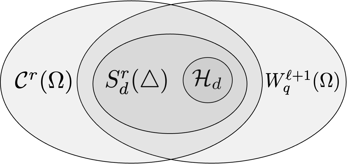
Note that we utilize SBB polynomials as basis to construct the homogeneous polynomial space of degree $d$, $\mathcal{H}_{d}$, over the whole domain $\Omega$. Then the smoothness constraint $\mathbf{M}\boldsymbol{\gamma}=\mathbf{0}$, along all the edges and vertices of all spherical triangles $\tau\in\triangle$, is imposed to restrict the function space of interest to $\mathcal{S}_{d}^{r}(\triangle)=\{s\in C^{r}(\Omega),s|_{\tau}\in\mathcal{H}_{d},\tau\in\triangle\}$. The mean function $m$ is assumed to reside in the spherical Sobolev space $W_{q}^{\ell+1}(\Omega)$, which is a superset of any polynomial function space when $\Omega$ is compact. The relationship between these function spaces is illustrated in Figure B.3.

Figure B.3: Relationship between function spaces $\mathcal{C}^{r}(\Omega),\mathcal{S}_{d}^{r}(\triangle),\mathcal{H}_{d}$ and $W_{q}^{\ell+1}(\Omega)$ for compact domain $\Omega$.

B.3. Example of Spherical Bernstein Basis (SBB) Polynomials

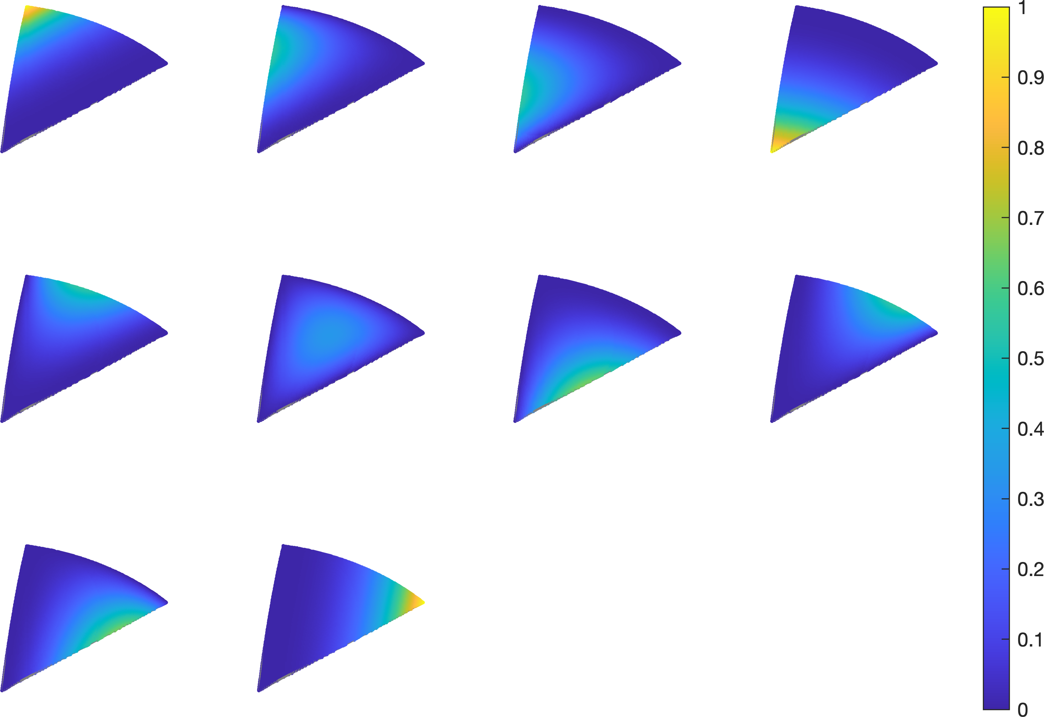
The SBB polynomials are defined as $B_{ijk}^{\tau}(\mathbf{x})=\frac{d!}{i!j!k!}b_{1}(\mathbf{x})^{i}b_{2}(\mathbf{x})^{j}b_{3}(\mathbf{x})^{k}$, $i+j+k=d$, $\tau\in\triangle$, where $b_{\kappa}(\mathbf{v})=\mathrm{vol}(\uptau_{\kappa})/\mathrm{vol}(\uptau)$ are the spherical barycentric coordinates. Here $\mathrm{vol}$ stands for volume, $\uptau_{\kappa}$ is tetrahedron $\langle\mathbf{0},\mathbf{v},\mathbf{v}_{\kappa+1},\mathbf{v}_{\kappa+2}\rangle$, and $\uptau$ is tetrahedron $\langle\mathbf{0},\mathbf{v}_{1},\mathbf{v}_{2},\mathbf{v}_{3}\rangle$. Illustrations of $\uptau$ and $\uptau_{1}$ are shown in Figure B.1. When $d=3$, there are ${d+2\choose 2}=10$ SBB polynomials of degree $3$, $\{B_{ijk}^{\tau}(\mathbf{x})\}_{i+j+k=d}$, see Figure B.4.

Figure B.4: SSB basis polynomials when $d=3$.

B.4. Proofs of Lemmas 1 – 2

In this section, we present preliminary results of SBB polynomials. Lemma B.0 establishes the stability of SBB over a single spherical triangle.

Lemma B.0.

Let $\boldsymbol{\gamma}=\{\gamma_{ijk}^{\tau},i+j+k=d,\tau\in\triangle\}\equiv\{\gamma_{\xi},\xi\in\mathcal{M}\}$ be the coefficients of SBB basis $\{B_{\xi},\xi\in\mathcal{M}\}$. Assume (C3) such that all triangles in the triangulation $\triangle$ are comparable in the sense that $c\max_{\tau\in\triangle}A_{\tau}\leq\min_{\tau\in\triangle}A_{\tau}$ for some constant $c>0$, then

$$\frac{1}{K^{2}}|\triangle|^{2}\|\boldsymbol{\gamma}\|_{2}^{2}\leq\|p\|_{\Omega}^{2}\leq 3^{2d}|\triangle|^{2}\|\boldsymbol{\gamma}\|_{2}^{2},$$

and equivalently

$$\frac{1}{K^{2}}N^{-1}\|\boldsymbol{\gamma}\|_{2}^{2}\leq\|p\|_{\Omega}^{2}\leq 3^{2d}N^{-1}\|\boldsymbol{\gamma}\|_{2}^{2}.$$

Proof.

By Assumption (C3), we have $\rho_{\tau}^{2}\leq A_{\tau}\leq|\triangle|^{2}\leq\rho^{2}\rho_{\tau}^{2}$ for all $\tau\in\triangle$, implying $A_{\tau}\asymp|\triangle|^{2}$. Let $\tau$ be a spherical triangle contained in a spherical cap of radius $1/2$, and let $1\leq q\leq\infty$. Then by Theorem 14.9 of Lai and Schumaker (2007), for any SBB polynomial $p=\sum_{i+j+k=d}\gamma_{ijk}^{\tau}B_{ijk}^{\tau}$ of degree $d$, we have ${K}^{-1}A_{\tau}^{1/q}\|\boldsymbol{\gamma}^{\tau}\|_{q}\leq\|p\|_{q,\tau}\leq 3^{d}A_{\tau}^{1/q}\|\boldsymbol{\gamma}^{\tau}\|_{q}$, where constant $K$ only depends on $d$. Let $q=2$, we have $K^{-1}|\triangle|\|\boldsymbol{\gamma}^{\tau}\|_{2}\leq\|p\|_{2,\tau}\leq 3^{d}|\triangle|\|\boldsymbol{\gamma}^{\tau}\|_{2}$. Further, we can extend the result to the closure of $\Omega\subseteq\mathbb{S}^{2}$, $K^{-2}|\triangle|^{2}\|\boldsymbol{\gamma}\|_{2}^{2}\leq\|p\|_{L^{2}(\Omega)}^{2}\leq 3^{2d}|\triangle|^{2}\|\boldsymbol{\gamma}\|_{2}^{2}$. In addition, by Assumption (C1), we have

$$c\|p\|_{L^{2}(\Omega)}\leq\|p\|_{\Omega}^{2}\leq C\|p\|_{L^{2}(\Omega)},$$ (B.1)

for some positive constants $0<c,C<\infty$. Therefore, the lemma is proved. ∎

Proof of Lemma 1.

By the definition of $\|\cdot\|_{n,\Omega}$ and $\|\cdot\|_{\Omega}$, we have

$$\langle p_{1},p_{2}\rangle_{n,\Omega} =\frac{1}{n}\sum_{i=1}^{n}\left\{\sum_{\xi_{1}\in\mathcal{M}}\gamma_{\xi_{1}}B_{\xi_{1}}(\mathbf{X}_{i})\right\}\left\{\sum_{\xi_{2}\in\mathcal{M}}\tilde{\gamma}_{\xi_{2}}B_{\xi_{2}}(\mathbf{X}_{i})\right\}=\sum_{\xi_{1},\xi_{2}\in\mathcal{M}}\gamma_{\xi_{1}}\tilde{\gamma}_{\xi_{2}}\langle B_{\xi_{1}},B_{\xi_{2}}\rangle_{n,\Omega},$$

$$\|p_{1}\|_{\Omega}^{2} =\sum_{\xi_{1},\xi_{1}^{\prime}}\gamma_{\xi_{1}}\tilde{\gamma}_{\xi_{1}^{\prime}}\langle B_{\xi_{1}},B_{\xi_{1}^{\prime}}\rangle_{\Omega},\quad\|p_{2}\|_{\Omega}^{2}=\sum_{\xi_{2},\xi_{2}^{\prime}}\gamma_{\xi_{2}}\tilde{\gamma}_{\xi_{2}^{\prime}}\langle B_{\xi_{2}},B_{\xi_{2}^{\prime}}\rangle_{\Omega}.$$

By Lemma B.0, we have

$$\frac{1}{NK^{2}}\left\{\sum_{\xi_{1}\in\mathcal{M}}\gamma_{\xi_{1}}^{2}\right\}^{1/2}\left\{\sum_{\xi_{2}\in\mathcal{M}}\tilde{\gamma}_{\xi_{2}}^{2}\right\}^{1/2}\leq\|p_{1}\|_{\Omega}\|p_{2}\|_{\Omega}\leq\frac{3^{2d}}{N}\left\{\sum_{\xi_{1}\in\mathcal{M}}\gamma_{\xi_{1}}^{2}\right\}^{1/2}\left\{\sum_{\xi_{2}\in\mathcal{M}}\tilde{\gamma}_{\xi_{2}}^{2}\right\}^{1/2}.$$

Therefore, by Cauchy-Schwarz inequality,

$$R_{n} =\frac{|\langle p_{1},p_{2}\rangle_{n,\Omega}-\langle p_{1},p_{2}\rangle_{\Omega}|}{\|p_{1}\|_{\Omega}\|p_{2}\|_{\Omega}}$$

$$\leq\frac{\sum_{\xi_{1},\xi_{2}\in\mathcal{M}}|\gamma_{\xi_{1}}\tilde{\gamma}_{\xi_{2}}|}{N^{-1}\left\{\sum_{\xi_{1}\in\mathcal{M}}\gamma_{\xi_{1}}^{2}\sum_{\xi_{2}\in\mathcal{M}}\tilde{\gamma}_{\xi_{2}}^{2}\right\}^{1/2}}\max_{\xi_{1},\xi_{2}\in\mathcal{M}}\left|\langle B_{\xi_{1}},B_{\xi_{2}}\rangle_{n,\Omega}-\langle B_{\xi_{1}},B_{\xi_{2}}\rangle_{\Omega}\right|$$

$$\leq C{N}\max_{\xi_{1},\xi_{2}\in\mathcal{M}}\left|\langle B_{\xi_{1}},B_{\xi_{2}}\rangle_{n,\Omega}-\langle B_{\xi_{1}},B_{\xi_{2}}\rangle_{\Omega}\right|.$$

It only remains to prove

$$\max_{\xi_{1},\xi_{2}\in\mathcal{M}}\left|\langle B_{\xi_{1}},B_{\xi_{2}}\rangle_{n,\Omega}-\langle B_{\xi_{1}},B_{\xi_{2}}\rangle_{\Omega}\right|=O_{p}\left\{(\log n)^{1/2}(nN)^{-1/2}\right\}.$$

Let $Z_{i}=B_{\xi_{1}}(\mathbf{X}_{i})B_{\xi_{2}}(\mathbf{X}_{i})-{\mathrm{E}}\{B_{\xi_{1}}(\mathbf{X}_{i})B_{\xi_{2}}(\mathbf{X}_{i})\}$. We have ${\mathrm{E}}Z^{2}_{i}\asymp|\triangle|^{2}$. In addition, ${\mathrm{E}}|Z_{i}|^{k}\asymp{\mathrm{E}}|B_{\xi_{1}}(\mathbf{X}_{i})B_{\xi_{2}}(\mathbf{X}_{i})|^{k}\asymp|\triangle|^{2}\leq C2^{k-1}k!{\mathrm{E}}Z_{i}^{2}$, for some constant $0<C<\infty$. Thus, by union bound and Bernstein’s inequality, we have for large $t>0$,

$$\sum_{n=1}^{\infty}\mathrm{P}\left(\max_{\xi_{1},\xi_{2}\in\mathcal{M}}\left|\frac{1}{n}\sum_{i=1}^{n}\langle B_{\xi_{1}},B_{\xi_{2}}\rangle_{n,\Omega}-\langle B_{\xi_{1}},B_{\xi_{2}}\rangle_{\Omega}\right|\geq t\sqrt{\frac{\log n}{nN}}\right)$$

$$\leq |\mathcal{M}|^{2}\sum_{n=1}^{\infty}\mathrm{P}\left(\left|\frac{1}{n}\sum_{i=1}^{n}\langle B_{\xi_{1}},B_{\xi_{2}}\rangle_{n,\Omega}-\langle B_{\xi_{1}},B_{\xi_{2}}\rangle_{\Omega}\right|\geq t\sqrt{\frac{\log n}{nN}}\right)$$

$$\leq \sum_{n=1}^{\infty}|\mathcal{M}|^{2}\exp\left(\frac{-t^{2}}{4+2ct\sqrt{N\log n/n}}\right)\leq\sum_{n=1}^{\infty}|\mathcal{M}|^{2}n^{-4}<\sum_{n=1}^{\infty}n^{-2}<\infty.$$

The second last inequality holds due to $N\asymp cn^{\omega},\omega<1,c>0$ by Assumption (C3). With Borel-Cantelli lemma, we have

$$\max_{\xi_{1},\xi_{2}\in\mathcal{M}}\left|\frac{1}{n}\sum_{i=1}^{n}\langle B_{\xi_{1}},B_{\xi_{2}}\rangle_{n,\Omega}-\langle B_{\xi_{1}},B_{\xi_{2}}\rangle_{\Omega}\right|=O_{p}(\sqrt{\log n/nN}),$$

and the proof is completed. ∎

As a result of Lemma 1, we have

$$\left|\frac{\|p\|_{n,\Omega}^{2}-\|p\|_{\Omega}^{2}}{\|p\|_{\Omega}^{2}}\right|=\left|\frac{\|p\|_{n,\Omega}^{2}}{\|p\|_{\Omega}^{2}}-1\right|=O_{p}\left\{(N\log n)^{1/2}n^{-1/2}\right\},\text{ and }$$

$$c\|p\|_{\Omega}^{2}\leq\|p\|_{n,\Omega}^{2}\leq C\|p\|_{\Omega}^{2},~{}\text{ for some constants }0<c,C<\infty.$$ (B.2)

Proof of Lemma 2.

Firstly, let $1\leq q\leq\infty$. By Theorem 14.8 of Lai and Schumaker (2007), for any $\tau$ contained in a spherical cap of radius $1/2$ and $p\in\mathcal{S}_{d}^{r}(\tau)$, there exists a constant $K$ depending only on $d,q,$ and the smallest angle of $\tau$, such that $A_{\tau}^{-1/q}\|p\|_{q,\tau}\leq\|p\|_{\infty,\tau}\leq KA_{\tau}^{-1/q}\|p\|_{q,\tau}$. Here $A_{\tau}$ is the area of $\tau$, and of order $|\triangle|^{2}$. Let $q=2$, we have

$$\|p\|_{\infty,\Omega}\leq\sum_{\tau\in\triangle}\|p\|_{\infty,\tau}\leq\sum_{\tau\in\triangle}\frac{K}{|\triangle|}\|p\|_{2,\tau}\asymp\frac{K}{|\triangle|}\|p\|_{L^{2}(\Omega)}\asymp KN^{1/2}\|p\|_{L^{2}(\Omega)}.$$ (B.3)

Equations (B.1), (B.2) and (B.3) together imply $\|p\|_{\infty,\Omega}\leq N^{1/2}\|p\|_{\Omega}\leq N^{1/2}\|p\|_{n,\Omega}$, completing the first part of Lemma 2.

Secondly, by Theorem 14.21 of Lai and Schumaker (2007), for any $\tau$ with $|\tau|<1$, we have $|p|_{\ell,q,\tau}\leq K\rho_{\tau}^{-\ell}\|p\|_{q,\tau}$. Let $q=2,\ell=2<d$, by Assumption (C2), we have $\|p\|_{\mathcal{E},\tau}\leq K\rho_{\tau}^{-2}\|p\|_{2,\tau}\leq K|\triangle|^{-2}\|p\|_{2,\tau}$. Take summation over $\tau\in\triangle$, we have

$$\|p\|_{\mathcal{E},\Omega}\leq\frac{K}{|\triangle|^{2}}\|p\|_{L^{2}(\Omega)}\asymp{KN\|p\|_{L^{2}(\Omega)}},$$ (B.4)

which completes the second part of the lemma by applying Equations (B.1) – (B.2). ∎

B.5. Minimal determining set and approximation power of spherical splines

To extend our results on a single spherical triangle $\tau$ (or a local spherical domain) to the whole triangulation $\triangle$ (or a large spherical domain), we make use of Minimal Determining Set (MDS). A local MDS, $\mathcal{M}$, is the determining set for $\mathcal{S}$ with the smallest cardinality, such that if $s\in\mathcal{S}$, and the B-coefficients $c_{\xi}(s)=0$ for all $\xi\in\mathcal{M}$, then $s\equiv 0$. Here $\mathcal{S}\subseteq\mathcal{S}_{d}^{0}(\triangle)$ is the set of functions defined over $\triangle$. Such construction enables us to consider a local set of points, other than which, the B-coefficients are fully dependent on those in $\mathcal{M}$ through smoothness conditions. We also define $\text{star}(v):=\text{star}^{1}(v)$ to be the set of all triangles sharing the vertex $v$, and $\text{star}^{j}(v):=\cup\{\text{all triangles sharing vertices of those in }\text{star}^{j-1}(v)\}$. Similarly, for a triangle, $\tau$, we define $\text{star}^{0}(\tau):=\tau$, and $\text{star}^{j}(\tau):=\cup\{\text{star}(v):v\in\text{star}^{j-1}(\tau)\}$.

In the main paper and the rest of this supplementary material, we focus on local and stable MDS. We say an MDS, $\mathcal{M}$, is local if there exists a constant $\curlywedge$ not depending on $\triangle$, such that $\Gamma_{\eta}$ is contained in $\text{star}^{\curlywedge}(\tau_{\eta})$, for all $\eta\in\mathcal{D}_{d,\triangle}\backslash\mathcal{M}$, where $\Gamma_{\eta}$ consists of all the domain points whose B-coefficients affect the B-coefficient $\eta$, and $\tau_{\eta}$ is the triangle containing $\eta$. The lower $\curlywedge$ is, the more locally defined a function is relative to $\triangle$. In addition, we say an MDS, $\mathcal{M}$, is stable if there exists a constant $K$ depending only on $\curlywedge$ and the smallest angle in $\triangle$, such that $|c_{\eta}|\leq K\max_{\xi\in\Gamma_{\eta}}|c_{\xi}|$, for all $\eta\in\mathcal{D}_{d,\triangle}\backslash\mathcal{M}$. The construction of MDS, local MDS, and stable MDS are illustrated in Figure B.5, also see in Definition 13.38 of Lai and Schumaker (2007).

Figure B.5: Illustration of local stable MDS construction. Note $\mathcal{M}$ is not necessarily unique, and $|\mathcal{M}|=\text{dim}\mathcal{S}$; $\Gamma_{\eta}=\{\xi\in\mathcal{M}:c_{\eta}(s)$ depends on $c_{\xi}(s)\}$ is the set of domain points in $\mathcal{M}$ whose B-coefficients affects $c_{\eta}$; $\tau_{\eta}$ is the triangle that contains $\eta$.

Lemma B.0 establishes the local approximation power of the spherical splines for functions defined over a triangulation $\triangle\subseteq\mathbb{S}^{2}$.

Lemma B.0 (Theorem 14.22 of Lai and Schumaker (2007)).

Suppose $\mathcal{M}$ is a stable local MDS for a spherical spline space $\mathcal{S}\subseteq\mathcal{S}^{0}_{d}(\triangle)$, and $\Omega\subseteq\mathbb{S}^{2}$ is the domain of interest. The triangulation $\triangle$ covers all or part of $\mathbb{S}^{2}$. We consider a quasi-interpolation operator $Q:L_{1}(\Omega)\to\mathcal{S}$ which yields a spline $s=Qf$ for any $f\in L_{1}(\mathbb{S}^{2})$. We can construct $s$ by assigning a coefficient functional to $f$ calculated by solving the B-coefficients corresponding to $\xi\in\mathcal{M}$, see Figure B.6. Then $Q:L_{1}(\Omega)\to\mathcal{S}$ is a linear projector such that for any triangle $\tau\in\triangle$ and $1\leq q\leq\infty$, $\|Qf\|_{q,\tau}\leq K\|f\|_{q,\Omega_{\tau}},\quad\forall f\in L_{1}(\Omega_{\tau}),$ where $\Omega_{\tau}=\text{star}^{\curlywedge}(\tau)$. The constant $K$ depends on $d,\curlywedge,$ and the smallest angle in $\Omega_{\tau}$.

Figure B.6: Illustration of quasi-interpolation operator $Q$. Here $c_{\xi}(f)=\gamma_{\xi}(F_{d,\tau_{\xi}}f)$ is the B-coefficients corresponding to $\xi$, $\tau_{\xi}$ is the triangle that contains $\xi$, $F_{d,\tau_{\xi}}f$ is the averaged Taylor polynomial of degree $d$ associated with $\tau_{\xi}$; $c_{\eta}(f)$ is a linear combination of $\{c_{\xi}(f)\}_{\xi\in\mathcal{M}_{\eta}}$, $\mathcal{M}_{\eta}\subseteq\text{star}^{\curlywedge}(\tau_{\eta})$, $\tau_{\eta}$ is the triangle that contains $\eta$.

Now we are ready to derive the global approximation power of SBB polynomials in Lemma B.0 and Lemma B.0 using Lemma B.0.

Lemma B.0 (Theorem 14.24 Lai and Schumaker (2007)).

Assume the constant $\curlywedge$ and the mesh size $|\triangle|$ satisfies $\curlywedge|\triangle|\leq 1$. Let $0\leq\ell\leq d$ with $\ell=d(\bmod 2)$. Then for $f\in W_{q}^{\ell+1}(\Omega)$ with $1\leq q\leq\infty$, $|f-Qf|_{k,q,\Omega}\leq K|\triangle|^{\ell+1-k}|f|_{\ell+1,q,\Omega}$, for all $0\leq k\leq\ell$. If $\Omega$ covers $\mathbb{S}^{2}$, the constant $K$ depends only on $d$ and the smallest angle in the triangles of $\triangle$. Otherwise, $K$ may also depend on the Lipschitz constant of $\partial\Omega$.

Remark B.0.

When $d$ and $\ell$ are both even or both odd, $\ell=d(\mathrm{mod}2)$. Otherwise, $\ell\neq d(\mathrm{mod}2)$, where the approximation power in the above lemma cannot be gauranteed. This issue can be circumvented by considering the approximation function space $\{f=c_{1}f_{1}+c_{2}f_{2}:f_{1}\in S_{d}^{r}(\triangle),f_{2}\in\mathcal{S}_{d-1}^{r}(\triangle)\}$, see Baramidze et al. (2006).

Next, we extend the results above to $\mathcal{S}_{d}^{r}(\triangle)$. In particular, we can construct a triangulation such that $\curlywedge=3,|\triangle|\leq 1/6$, which satisfies the condition $\curlywedge|\triangle|\leq 1$, and leads to Lemma B.0.

Lemma B.0 (Theorem 14.26 Lai and Schumaker (2007)).

Let $0\leq\ell\leq d$ with $\ell=d(\bmod 2)$. Suppose $\triangle$ is a spherical triangulation of a set $\Omega$ on $\mathbb{S}^{2}$, and that $|\triangle|\leq 1/6$. Let $d\geq 3r+2$. Suppose $f\in W_{q}^{\ell+1}(\Omega)$ with $1\leq q\leq\infty$. Then there exists a spline $s\in\mathcal{S}_{d}^{r}(\triangle)$ such that $|f-s|_{k,q,\Omega}\leq K|\triangle|^{\ell+1-k}|f|_{\ell+1,q,\Omega}$, for all $0\leq k\leq\ell$. If $\Omega$ covers $\mathbb{S}^{2}$, the constant $K$ depends only on $d$ and the smallest angle in the triangles of $\triangle$. Otherwise, $K$ may also depend on the Lipschitz constant of $\partial\Omega$.

This lemma gives the global approximation power of spherical splines. By assuming $|f|_{\ell+1,2,\Omega}$ being a finite constant, the residual of spline approximation can be bounded with order $|\triangle|^{\ell+1}$. Let $k=2,q=\infty$, Lemma B.0 implies

$$|f-s|_{2,\infty,\Omega}\leq K|\triangle|^{\ell-1}|f|_{\ell+1,\infty,\Omega}.$$ (B.5)

Let $k=0,q=\infty$, Lemma B.0 implies

$$\|f-s\|_{\infty,\Omega}\leq K|\triangle|^{\ell+1}|f|_{\ell+1,\infty,\Omega}.$$ (B.6)

B.6. Size of bias and noise terms

In this section, we study the asymptotics of the bias and noise terms, and provide proof for 1 and 2.

To prepare for the proof, we consider $\mathcal{B}(\Omega)$ the space of all bounded real-valued functions over $\Omega=\cup_{\tau\in\triangle}\tau$. By definitions (4), (6) and (7),

$$s_{\lambda} =\operatorname*{arg\,min}_{s\in\mathcal{S}}n\|m(\mathbf{x})+\sigma(\mathbf{x})\epsilon-s(\mathbf{x})\|_{n,\Omega}^{2}+\lambda\|s(\mathbf{x})\|_{\mathcal{E}}^{2},$$ (B.7)

$$s_{\lambda,m} =\operatorname*{arg\,min}_{s\in\mathcal{S}}n\|m(\mathbf{x})-s(\mathbf{x})\|_{n,\Omega}^{2}+\lambda\|s(\mathbf{x})\|_{\mathcal{E}}^{2},$$ (B.8)

$$s_{\lambda,\epsilon} =\operatorname*{arg\,min}_{s\in\mathcal{S}}n\|\sigma(\mathbf{x})\epsilon-s(\mathbf{x})\|_{n,\Omega}^{2}+\lambda\|s(\mathbf{x})\|_{\mathcal{E}}^{2}.$$ (B.9)

Proof of 1.

By triangle inequality and definition of $V_{n}$,

$$\|s_{\lambda,m}-m\|_{\infty,\Omega}\leq\|m-s_{0,m}\|_{\infty,\Omega}+\|s_{\lambda,m}-s_{0,m}\|_{\infty,\Omega}\leq\|m-s_{0,m}\|_{\infty,\Omega}+V_{n}\|s_{\lambda,m}-s_{0,m}\|_{n,\Omega}.$$

By (B.8), for any $u\in\mathcal{S}_{d}^{r}(\triangle)$ and $t\in\mathbb{R}$,

$$n\|m-(s_{\lambda,m}+tu)\|_{n,\Omega}^{2}+\lambda\|s_{\lambda,m}+tu\|_{\mathcal{E}}^{2} \geq n\|m-s_{\lambda,m}\|_{n,\Omega}^{2}+\lambda\|s_{\lambda,m}\|_{\mathcal{E}}^{2},$$

$$n\|m-(s_{0,m}+tu)\|_{n,\Omega}^{2} \geq n\|m-s_{0,m}\|_{n,\Omega}^{2}.$$

It follows that $s_{\lambda,m}$ is characterized by the orthogonality relationship

$$n\langle m-s_{\lambda,m},u\rangle_{n,\Omega}=\lambda\langle s_{\lambda,m},u\rangle_{\mathcal{E}},\quad\text{ for all }u\in\mathcal{S}_{d}^{r}(\triangle),$$ (B.10)

while $s_{0,m}$ is characterized by

$$n\langle m-s_{0,m},u\rangle_{n,\Omega}=0,\quad\text{ for all }u\in\mathcal{S}.$$ (B.11)

By taking the difference of (B.10) and(B.11), we have $n\langle s_{0,m}-s_{\lambda,m},u\rangle_{n,\Omega}=\lambda\langle s_{\lambda,m},u\rangle_{\mathcal{E}}$. Plug in $u=s_{0,m}-s_{\lambda,m}$, we have

$$0 \leq n\|s_{0,m}-s_{\lambda,m}\|_{n,\Omega}^{2}=\lambda\langle s_{\lambda,m},s_{0,m}-s_{\lambda,m}\rangle_{\mathcal{E}}\leq\lambda(\langle s_{0,m},s_{\lambda,m}\rangle_{\mathcal{E}}-\|s_{\lambda,m}\|_{\mathcal{E}}^{2}),$$

and $\|s_{\lambda,m}\|^{2}_{\mathcal{E}}\leq\langle s_{0,m},s_{\lambda,m}\rangle_{\mathcal{E}}\leq\|s_{\lambda,m}\|_{\mathcal{E}}\|s_{0,m}\|_{\mathcal{E}}$. By Cauchy-Schwarz inequality,

$$n\|s_{0,m}-s_{\lambda,m}\|_{n,\Omega}^{2} =\lambda\langle s_{\lambda,m},s_{0,m}-s_{\lambda,m}\rangle_{\mathcal{E}}\leq\lambda\|s_{\lambda,m}\|_{\mathcal{E}}\cdot\|s_{0,m}-s_{\lambda,m}\|_{\mathcal{E}}$$

$$\leq\lambda\|s_{\lambda,m}\|_{\mathcal{E}}\cdot\overline{V}_{n}\|s_{0,m}-s_{\lambda,m}\|_{n,\Omega},$$

which implies that $\|s_{0,m}-s_{\lambda,m}\|_{n,\Omega}\leq n^{-1}\lambda\overline{V}_{n}\|s_{\lambda,m}\|_{\mathcal{E}}.$ With (B.5),

$$\|s_{0,m}-s_{\lambda,m}\|_{\infty,\Omega} \leq n^{-1}\lambda\overline{V}_{n}V_{n}\|s_{\lambda,m}\|_{\mathcal{E}}\leq n^{-1}\lambda\overline{V}_{n}V_{n}\|s_{0,m}\|_{\mathcal{E}}$$

$$\leq n^{-1}\lambda\overline{V}_{n}V_{n}(\|m-s_{0,m}\|_{\mathcal{E}}+\|m\|_{\mathcal{E}})$$

$$\leq n^{-1}\lambda{N^{3/2}}\left(K|\triangle|^{\ell-1}|m|_{\ell+1,\infty,\Omega}+|m|_{2,\infty,\Omega}\right).$$

And (B.6) entails $\|m-s_{0,m}\|_{\infty,\Omega}\leq K|\triangle|^{\ell+1}|m|_{\ell+1,\infty,\Omega}.$ Therefore,

$$\|s_{\lambda,m}-m\|_{\infty,\Omega} \leq\|m-s_{0,m}\|_{\infty,\Omega}+\|s_{0,m}-s_{\lambda,m}\|_{\infty,\Omega}$$

$$=O_{p}\left\{|\triangle|^{\ell+1}|m|_{\ell+1,\infty,\Omega}+\frac{\lambda{N^{3/2}}}{n}\left(|\triangle|^{\ell-1}|m|_{\ell+1,\infty,\Omega}+|m|_{2,\infty,\Omega}\right)\right\}$$

$$=O_{p}\left\{N^{-(\ell+1)/2}|m|_{\ell+1,\infty,\Omega}+\frac{\lambda{N^{3/2}}}{n}\left(N^{-(\ell-1)/2}|m|_{\ell+1,\infty,\Omega}+|m|_{2,\infty,\Omega}\right)\right\}$$

$$=O_{p}\left\{\frac{\lambda{N^{3/2}}}{n}|m|_{2,\infty,\Omega}+\left(1+\frac{\lambda{N^{5/2}}}{n}\right)N^{-(\ell+1)/2}|m|_{\ell+1,\infty,\Omega}\right\}.$$

The proof is completed. ∎

Proof of 2 (Part 1).

The key is to recognize the orthogonal relation that characterizes $m_{\lambda,\epsilon}$. By (B.9), for any $u\in\mathcal{S}_{d}^{r}(\triangle)$ and $t\in\mathbb{R}$,

$$n\|\sigma(\mathbf{x})\epsilon-(s_{\lambda,\epsilon}+tu)\|_{n,\Omega}^{2}+\lambda\|s_{\lambda,\epsilon}+tu\|_{\mathcal{E}}^{2} \geq n\|\sigma(\mathbf{x})\epsilon-s_{\lambda,\epsilon}\|_{n,\Omega}^{2}+\lambda\|s_{\lambda,\epsilon}\|_{\mathcal{E}}^{2}.$$

It follows that $s_{\lambda,\epsilon}$ is characterized by

$$n\langle s_{\lambda,\epsilon}-\sigma(\mathbf{x})\epsilon,u\rangle_{n,\Omega}+\lambda\langle s_{\lambda,\epsilon},u\rangle_{\mathcal{E}}=0,\quad\forall u\in\mathcal{S}_{d}^{r}(\triangle).$$

Note that we can write $s_{\lambda,\epsilon}$ in terms of SBB basis $\{B_{\xi},\xi\in\mathcal{M}\}$, $s_{\lambda,\epsilon}(\mathbf{x})=\sum_{\xi\in\mathcal{M}}c_{s_{\lambda,\epsilon},\xi}B_{\xi}(\mathbf{x})$, where $c_{s_{\lambda,\epsilon},\xi}$ are the B-coefficients. Let $u=B_{\xi}(\mathbf{X}_{i})$, we have $\sum_{i=1}^{n}s_{\lambda,\epsilon}(\mathbf{X}_{i})B_{\xi}(\mathbf{X}_{i})+\lambda\langle s_{\lambda,\epsilon},B_{\xi}\rangle_{\mathcal{E}}=\sum_{i=1}^{n}B_{\xi}(\mathbf{X}_{i})\sigma(\mathbf{X}_{i})\epsilon_{i}$ for all $\xi\in\mathcal{M}$. Multiply both sides by $c_{s_{\lambda,\epsilon},\xi}/n$, and perform summation over $\xi\in\mathcal{M}$. We have, by Cauchy-Schwarz inequality,

$$\|s_{\lambda,\epsilon}\|_{n,\Omega}^{2} \leq\|s_{\lambda,\epsilon}\|_{n,\Omega}^{2}+\frac{\lambda}{n}\mathcal{E}(s_{\lambda,\epsilon})=\frac{1}{n}\sum_{\xi\in\mathcal{M}}c_{s_{\lambda,\epsilon},\xi}\sum_{i=1}^{n}B_{\xi}(\mathbf{X}_{i})\sigma(\mathbf{X}_{i})\epsilon_{i}$$

$$\leq\left(\sum_{\xi\in\mathcal{M}}|c_{s_{\lambda,m},\xi}|^{2}\right)^{1/2}\left[\sum_{\xi\in\mathcal{M}}\sum_{i=1}^{n}\left\{\frac{1}{n}B_{\xi}(\mathbf{X}_{i})\sigma(\mathbf{X}_{i})\epsilon_{i}\right\}^{2}\right]^{1/2}.$$

Apply Lemma B.0, we have

$$\|s_{\lambda,\epsilon}\|_{n,\Omega}^{2} \leq K{N^{1/2}}\|s_{\lambda,\epsilon}\|_{\Omega}\left[\sum_{\xi\in\mathcal{M}}\sum_{i=1}^{n}\left\{\frac{1}{n}B_{\xi}(\mathbf{X}_{i})\sigma(\mathbf{X}_{i})\epsilon_{i}\right\}^{2}\right]^{1/2}.$$

In addition, by Lemma 1, we have $\sup_{p\in\mathcal{S}_{d}^{r}(\triangle)}|\|p\|_{n,\Omega}^{2}/\|p\|_{\Omega}^{2}-1|=O_{p}\{(N\log n)^{1/2}n^{-1/2}\}$, which implies

$$\|s_{\lambda,\epsilon}\|_{\Omega}^{2}\leq\|s_{\lambda,\epsilon}\|_{n,\Omega}^{2}+\left(\frac{N\log n}{n}\right)^{1/2}\|s_{\lambda,\epsilon}\|_{\Omega}^{2}$$

$$\leq K{N^{1/2}}\|s_{\lambda,\epsilon}\|_{\Omega}\left[\sum_{\xi\in\mathcal{M}}\sum_{i=1}^{n}\left\{\frac{1}{n}B_{\xi}(\mathbf{X}_{i})\sigma(\mathbf{X}_{i})\epsilon_{i}\right\}^{2}\right]^{1/2}+\left(\frac{N\log n}{n}\right)^{1/2}\|s_{\lambda,\epsilon}\|_{\Omega}^{2}.,$$ (B.12)

By Lemma 14.8 of Lai and Schumaker (2007) and (C4), $\|p\|_{\tau}\asymp\|p\|_{L^{2}(\tau)}\leq N^{-1/2}\|p\|_{\infty,\tau},\forall p\in\mathcal{S}_{d}^{r}(\triangle)$. Then, by the law of large number,

$$\frac{1}{n}\sum_{i=1}^{n}\left\{B_{\xi}(\mathbf{X}_{i})\sigma(\mathbf{X}_{i})\epsilon_{i}\right\}^{2} ={\mathrm{E}}(B_{\xi}(\mathbf{X})^{2}\sigma(\mathbf{X})^{2}\epsilon(\mathbf{X})^{2})+o_{p}(1)$$

$$={\mathrm{E}}(B_{\xi}(\mathbf{X})^{2}\sigma(\mathbf{X})^{2})+o_{p}(1)$$

$$\leq K\|B_{\xi}(\mathbf{X})\sigma(\mathbf{X})\|_{L^{2}(\Omega)}^{2}$$

$$\leq KN^{-1}\|B_{\xi}(\mathbf{X})\sigma(\mathbf{X})\|_{\infty,\tau^{*}}^{2}=O_{p}(N^{-1}),$$ (B.13)

where $\tau^{*}$ is the triangle where $B_{\xi}(\mathbf{X})$ has positive values. By Assumption (C5), we have $N=Cn^{\omega},\omega<1$. Note $|\mathcal{M}|=N(d+1)(d+2)/2\asymp N$. By (B.1), (B.12) and (B.13),

$$\left\{1-\left(\frac{N\log n}{n}\right)^{1/2}\right\}\|s_{\lambda,\epsilon}\|_{L^{2}(\Omega)}\leq KN^{1/2}{({|\mathcal{M}|}/{nN})^{1/2}}=O_{p}\left(n^{-1/2}N^{1/2}\right).$$

The proof is completed by noticing $\left(\frac{N\log n}{n}\right)^{1/2}\to 0$ as $n\to\infty$. ∎

To prepare for Part 2 of 2, we first introduce the following two lemmas. Let $\boldsymbol{\Gamma}_{\lambda}$ be the symmetric positive definite matrix

$$\left[\frac{1}{n}\sum_{i=1}^{n}B_{\xi_{1}}(\mathbf{X}_{i})B_{\xi_{2}}(\mathbf{X}_{i})+\frac{\lambda}{n}\langle B_{\xi_{1}},B_{\xi_{2}}\rangle_{\mathcal{E}}\right]_{\xi_{1},\xi_{2}\in\mathcal{M}}.$$ (B.14)

In particular, when $\lambda=0$, we have $\boldsymbol{\Gamma}_{0}=\left[\frac{1}{n}\sum_{i=1}^{n}B_{\xi_{1}}(\mathbf{X}_{i})B_{\xi_{2}}(\mathbf{X}_{i})\right]_{\xi_{1},\xi_{2}\in\mathcal{M}}$.

Lemma B.0.

Under Assumptions (C3), (C4), and (C5), for $\boldsymbol{\Gamma}_{\lambda}$, we have the following asymptotic results.

• As $n\to\infty$, with probability one,

  $$cN^{-1}\leq\rho_{\min}(\boldsymbol{\Gamma}_{\lambda})\leq\rho_{\max}(\boldsymbol{\Gamma}_{\lambda})\leq C\left(N^{-1}+\lambda N/n\right),$$

  holds for some constants $0<c<C<\infty$ depending on $\lambda$.

• There exists a constant $C>0$ depending on $d$ such that $\|\boldsymbol{\Gamma}_{\lambda}^{{-1}}\|_{\infty}\leq CN$.

• For any vector $\boldsymbol{\sigma}=(\sigma_{1},\ldots,\sigma_{n})^{\top}$, there exists a constant $C>0$ depending on $d$, such that $\left\|\mathbf{B}^{\top}(\mathbf{x})\boldsymbol{\Gamma}_{\lambda}^{-1}\frac{1}{n}\sum_{n=1}^{n}\mathbf{B}(\mathbf{X}_{i})\sigma_{i}\right\|_{\infty}\leq C\|\boldsymbol{\sigma}\|_{\infty}.$

Proof.

(i) For any $\boldsymbol{\gamma}\in{\mathbb{R}}^{|\mathcal{M}|}$, let $p(\mathbf{x})=\mathbf{B}^{\top}(\mathbf{x})\boldsymbol{\gamma}\in\mathcal{S}_{d}^{r}(\triangle)$. Note that

$$\boldsymbol{\gamma}^{\top}\boldsymbol{\Gamma}_{\lambda}\boldsymbol{\gamma}=\boldsymbol{\gamma}^{\top}\frac{1}{n}\sum_{i=1}^{n}\mathbf{B}(\mathbf{X}_{i})\mathbf{B}^{\top}(\mathbf{X}_{i})\boldsymbol{\gamma}+\boldsymbol{\gamma}^{\top}\frac{\lambda}{n}|\langle B_{\xi_{1}},B_{\xi_{2}}\rangle_{\mathcal{E}}|_{\xi_{1},\xi_{2}\in\mathcal{M}}\boldsymbol{\gamma}=\|p\|_{n,\Omega}^{2}+\frac{\lambda}{n}\|p\|_{\mathcal{E}}^{2}.$$

By Lemma 1, we have $|\|p\|_{n,\Omega}^{2}/\|p\|_{2,\Omega}^{2}-1|\leq R_{n}$. And by Lemma B.0,

$$c(1-R_{n})N^{-1}\|\boldsymbol{\gamma}\|_{2}^{2}\leq(1-R_{n})\|p\|_{L^{2}(\Omega)}^{2}\leq\|p\|_{n,\Omega}^{2}\leq(1+R_{n})\|p\|_{L^{2}(\Omega)}^{2}\leq C(1+R_{n})N^{-1}\|\boldsymbol{\gamma}\|_{2}^{2}.$$

It follows that $\rho_{\min}(\boldsymbol{\Gamma}_{\lambda})\geq cN^{-1}$ for some $c>0$. By Lemma 2, $\|p\|_{\mathcal{E}}^{2}\leq CN^{2}\|p\|_{\Omega}^{2}$. By Lemma B.0, we have $\|p\|_{\Omega}^{2}\leq CN^{-1}\|\boldsymbol{\gamma}\|_{2}^{2}$. Combining the bounds for $\|p\|_{n,\Omega}^{2}$ and $\|p\|_{\mathcal{E}}^{2}$ gives

$$\rho_{\max}(\boldsymbol{\Gamma}_{\lambda})\leq C\left\{(1+R_{n})N^{-1}+\frac{\lambda N}{n}\right\}\leq C\left(N^{-1}+\lambda N/n\right).$$

(ii) We know $\boldsymbol{\Gamma}_{\lambda}$ is an invertible symmetric matrix from (i), with condition number $1<\kappa=\rho_{\max}(\boldsymbol{\Gamma}_{\lambda})/\rho_{\min}(\boldsymbol{\Gamma}_{\lambda})<C$, for some constant $C>1$. We then make use of properties of banded matrix. A matrix $\mathbf{M}=(M_{ij})$ is said to be banded with bandwidth $b$ if $M_{ij}=0$ for $|i-j|\geq b$, where $b$ is the smallest integer satisfying the condition. By construction of $B_{\xi}$, the bandwidth of $\boldsymbol{\Gamma}_{\lambda}$ is $\kappa=(d+1)(d+2)/2$. By Theorem 13.4.3 of DeVore and Lorentz (1993), $\|\boldsymbol{\Gamma}_{\lambda}^{-1}\|_{\infty}\leq 2\tau^{-2b}\|\boldsymbol{\Gamma}_{\lambda}^{-1}\|_{2}(1-\tau)^{-1}$, where $\tau=(\kappa^{2}-\kappa^{-2}+1)^{1/4b}<1$. Therefore, $\|\boldsymbol{\Gamma}_{\lambda}^{-1}\|_{\infty}\leq C\|\boldsymbol{\Gamma}_{\lambda}^{-1}\|_{2}\leq C\text{dim}(\boldsymbol{\Gamma}_{\lambda})\leq CN$, for some $C>0$.

(iii) Combining (i) and (ii), we have

$$\left\|\mathbf{B}^{\top}(\mathbf{x})\boldsymbol{\Gamma}_{\lambda}^{-1}\frac{1}{n}\sum_{i=1}^{n}\mathbf{B}(\mathbf{X}_{i})\sigma_{i}\right\|_{\infty}\leq C\|\boldsymbol{\sigma}\|_{\infty}.$$

The proof is completed. ∎

Lemma B.0.

Under Assumptions (C2) and (C5),

$$\|s_{0,\epsilon}\|_{\infty,\Omega}=O_{p}\left\{\sqrt{\frac{N\log n}{n}}\right\}.$$

Proof.

Note that $s_{0,\epsilon}=\sum_{\xi\in\mathcal{M}}\widehat{c}_{0,\xi}B_{\xi}(\mathbf{x})$. Since $B_{\xi}$ are bounded, by definition (7),

$$\|s_{0,\epsilon}\|_{\infty,\Omega}\leq c\|\widehat{\mathbf{c}}_{0}\|_{\infty}\asymp\left\|\boldsymbol{\Gamma}_{0}^{-1}\left[n^{-1}\sum_{i=1}^{n}B_{\xi}(\mathbf{X}_{i})\sigma(\mathbf{X}_{i})\epsilon_{i}\right]_{\xi\in\mathcal{M}}\right\|_{\infty,\Omega},\quad\widehat{\mathbf{c}}_{0}=\left(\widehat{c}_{0,\xi}\right)_{\xi\in\mathcal{M}}.$$

By Lemma B.0 (ii),

$$\|s_{0,\epsilon}\|_{\infty,\Omega}\leq C\|\boldsymbol{\Gamma}_{0}^{-1}\|_{\infty}\max_{\xi\in\mathcal{M}}\left|n^{-1}\sum_{i=1}^{n}B_{\xi}(\mathbf{X}_{i})\sigma(\mathbf{X}_{i})\epsilon_{i}\right|\leq CN\max_{\xi\in\mathcal{M}}\left|n^{-1}\sum_{i=1}^{n}B_{\xi}(\mathbf{X}_{i})\sigma(\mathbf{X}_{i})\epsilon_{i}\right|$$

holds almost surely. Therefore, it suffices to show

$$\max_{\xi\in\mathcal{M}}\left|n^{-1}\sum_{i=1}^{n}B_{\xi}(\mathbf{X}_{i})\sigma(\mathbf{X}_{i})\epsilon_{i}\right|=O_{p}\left\{(\log n)^{1/2}(nN)^{-1/2}\right\}.$$

Consider decomposing $\epsilon_{i}$ into a tail part $\epsilon_{i,1}^{D_{n}}$ and a truncated part $\epsilon_{i,2}^{D_{n}}$,

$$\epsilon_{i}=\epsilon_{i,1}^{D_{n}}+\epsilon_{i,2}^{D_{n}},\quad\epsilon_{i,1}^{D_{n}}=\epsilon_{i}\mathbbm{1}\{|\epsilon_{i}|>D_{n}\},\quad\epsilon_{i,2}^{D_{n}}=\epsilon_{i}\mathbbm{1}\{|\epsilon_{i}|\leq D_{n}\},$$

where $D_{n}=n^{\alpha}$ with $\max\{\frac{1}{2+\eta},\frac{1+\omega}{2(1+\eta)}\}<\alpha<{\frac{1-\omega}{2}}$. Note that $\eta$ defined in Assumption (C5) and $\omega$ defined in Assumption (C3) need to satisfy ${\omega<\frac{\eta}{\eta+2}}$ for the condition to be feasible.

Since ${\mathrm{E}}(\epsilon_{i})=0$, $|{\mathrm{E}}\{\epsilon_{i}\mathbbm{1}(|\epsilon_{i}|\leq D_{n})\}|=|{\mathrm{E}}\{\epsilon_{i}\mathbbm{1}(|\epsilon_{i}|>D_{n})\}|$. We then show $\mu^{D_{n}}:={\mathrm{E}}(\epsilon_{i,2}^{D_{n}})=-{\mathrm{E}}(\epsilon_{i,1}^{D_{n}})$ is bounded. By Assumption (C5),

$$|{\mathrm{E}}\{\epsilon_{i}\mathbbm{1}(|\epsilon_{i}|>D_{n})\}|\leq\left|{\mathrm{E}}\left\{\epsilon_{i}\frac{|\epsilon_{i}|^{1+\eta}}{D_{n}^{1+\eta}}\mathbbm{1}\left(|\epsilon_{i}|>D_{n}\right)\right\}\right|\leq\frac{1}{D_{n}^{1+\eta}}{\mathrm{E}}|\epsilon_{i}^{2+\eta}|\leq CD_{n}^{-(1+\eta)},$$

for $D_{n}$ large enough. By the boundedness of SBB and $\sigma$,

$$|B_{\xi}(\mathbf{X}_{i})\sigma(\mathbf{X}_{i})\mu^{D_{n}}|=O_{p}\{D_{n}^{-(1+\eta)}\}.$$ (B.15)

Here we use bound $\frac{1+\omega}{2(1+\eta)}<\alpha$ to ensure $D_{n}^{-(1+\eta)}\leq{\log n}^{1/2}(nN)^{-1/2}$.

Then, we prove the tail part $\epsilon_{i,1}^{D_{n}}$ vanishes almost surely. By Assumption (C5), ${\mathrm{E}}|\epsilon_{i}^{2+\eta}|\leq v_{\eta},\forall i$ for some $\eta>0$ and constant $v_{\eta}$. Therefore, by Markov’s inequality,

$$\sum_{n=1}^{\infty}\mathrm{P}\{|\epsilon_{n}|>D_{n}\}\leq\sum_{i=1}^{\infty}\frac{{\mathrm{E}}|\epsilon_{n}|^{2+\eta}}{D_{n}^{2+\eta}}\leq v_{\eta}\sum_{n=1}^{\infty}D_{n}^{-(2+\eta)}<\infty,$$

where the last inequality holds due to $\frac{1}{2+\eta}<\alpha$. By the Borel-Cantelli’s lemma, $\{|\epsilon_{n}|\leq D_{n}\}$ holds almost surely, for some $n$ large enough. Thus

$$\mathrm{P}\{w:\exists N(w),\text{ such that }|\epsilon_{n}(w)|\leq D_{n}\text{ for }n>N(w)\}=1.$$

Let $\epsilon^{*}=\max\{|\epsilon_{1}|,\ldots,|\epsilon_{n}|\}$, there exists $N^{*}(w)>N(w)$, such that $D_{N^{*}(w)}>\epsilon^{*}$. Since $D_{n}$ is an increasing function of $n$, we have $D_{n}>D_{N^{*}(w)}>\epsilon^{*}$, for $n>N^{*}(w)$. Then,

$$\mathrm{P}\{w:\exists N(w),\text{ such that }|\epsilon_{i}(w)|\leq D_{n},1\leq i\leq n,\text{ for }n>N(w)\}=1,$$

implying $\mathrm{P}\{w:\exists N(w),\text{ such that }|\epsilon_{i,1}^{D_{n}}|=0,1\leq i\leq n,\text{ for }n>N(w)\}=1.$ The boundedness of SBB and $\sigma$ leads to

$$|B_{\xi}(\mathbf{X}_{i})\sigma(\mathbf{X}_{i})\epsilon_{i,1}^{D_{n}}|=O_{a.s.}(n^{-k}),\forall k>0.$$ (B.16)

Finally, let $Z_{i}=\frac{1}{n}(\epsilon_{i,2}^{D_{n}}-\mu^{D_{n}})\sigma(\mathbf{X}_{i})B_{\xi}(\mathbf{X}_{i})$. Note that ${\mathrm{E}}(Z_{i})=0$, and

$$\mathrm{Var}(\epsilon_{i,2}^{D_{n}}-\mu^{D_{n}}) ={\mathrm{E}}(\epsilon_{i,2}^{D_{n}}-\mu^{D_{n}})^{2}={\mathrm{E}}\{\epsilon_{i}^{2}\mathbbm{1}(|\epsilon_{i}|\leq D_{n})\}-(\mu^{D_{n}})^{2}$$

$$={\mathrm{E}}(\epsilon_{i}^{2})-{\mathrm{E}}\{\epsilon_{i}^{2}\mathbbm{1}(|\epsilon_{i}|>D_{n})\}-(\mu^{D_{n}})^{2}$$

$$=1+O_{p}\left\{D_{n}^{-\eta}+D_{n}^{-2(1+\eta)}\right\}.$$

Note here the last inequality holds because ${\mathrm{E}}\{\epsilon_{i}^{2}\mathbbm{1}(|\epsilon_{i}|>D_{n})\}\leq{\mathrm{E}}|\epsilon_{i}^{2+\eta}|/D_{n}^{\eta}\leq v_{\eta}/D_{n}^{\eta}$ by Assumption (C5). By (B.13), ${\mathrm{E}}\{B_{\xi}^{2}(\mathbf{X})\sigma^{2}(\mathbf{X})\}=O_{p}(N^{-1})$. Since $\epsilon_{i,2}^{D_{n}}-\mu^{D_{n}}$ is independent from $B_{\xi}(\mathbf{X}_{i})$ given $\mathbf{X}_{i}$, and that $\{\epsilon_{i,2}^{D_{n}}-\mu^{D_{n}},1\leq i\leq n\}$ are independent from each other, we have ${\rm Var}(\sum_{i=1}^{n}Z_{i})=C{(nN)^{-1}}$ for some $C>0$. Note that $|\epsilon_{i,2}^{D_{n}}-\mu^{D_{n}}|<2D_{n}$, therefore

$${\mathrm{E}}|\epsilon_{i,2}^{D_{n}}-\mu^{D_{n}}|^{k}\leq 2^{k-2}D_{n}^{k-2}{\mathrm{E}}|\epsilon_{i,2}^{D_{n}}-\mu^{D_{n}}|^{2},~{}~{}~{}k\geq 2,$$

and

$${\mathrm{E}}|Z_{i}|^{k} =n^{-k}{\mathrm{E}}|\epsilon_{i,2}^{D_{n}}-\mu^{D_{n}}|^{k}{\mathrm{E}}|\sigma(\mathbf{X}_{i})B_{\xi}(\mathbf{X}_{i})|^{k}$$

$$\leq n^{-(k-2)}{\mathrm{E}}|\epsilon_{i,2}^{D_{n}}-\mu^{D_{n}}|^{k}\|B_{\xi}\|_{\infty,\Omega}^{k-2}{\mathrm{E}}|\sigma(\mathbf{X}_{i})B_{\xi}(\mathbf{X}_{i})|^{2}$$

$$\leq(2D_{n}n^{-1})^{k-2}k!{\mathrm{E}}Z_{i}^{2},$$

which implies $\{Z_{i}\}_{i=1}^{n}$ satisfies the Cramér’s condition with constant $c^{*}=2D_{n}n^{-1}$. By Bernstein’s inequality, for $\delta>0$ large enough, we have

$$\mathrm{P}\left(\left|\sum_{i=1}^{n}Z_{i}\right|\geq\delta\sqrt{\frac{\log n}{nN}}\right) \leq 2\exp\left\{\frac{-\delta^{2}\log n/nN}{4{\rm Var}(\sum_{i=1}^{n}Z_{i})+2c^{*}\delta\sqrt{\log n/nN}}\right\}$$

$$=2\exp\left(\frac{-\delta^{2}\log n/nN}{4c/nN+2c^{*}\delta\sqrt{\log n/nN}}\right)\leq 2n^{-3}.$$

For the last inequality to hold, we need $\alpha<\frac{1-\omega}{2}$. Therefore,

$$\sum_{n=1}^{\infty}\mathrm{P}\left(\max_{\xi\in\mathcal{M}}\left|\sum_{i=1}^{n}Z_{i}\right|\geq\delta\sqrt{\frac{\log n}{nN}}\right)\leq\frac{N}{2}(d+1)(d+2)\sum_{n=1}^{\infty}n^{-3}<\infty.$$

By applying Borel-Cantelli’s lemma,

$$\max_{\xi\in\mathcal{M}}\left|\sum_{i=1}^{n}Z_{i}\right|=\max_{\xi\in\mathcal{M}}\left|\sum_{i=1}^{n}\frac{1}{n}(\epsilon_{i,2}^{D_{n}}-\mu^{D_{n}})\sigma(\mathbf{X}_{i})B_{\xi}(\mathbf{X}_{i})\right|=O_{a.s.}\left(\sqrt{\frac{\log n}{nN}}\right)$$ (B.17)

The proof is completed by combining (B.15), (B.16) and (B.17). ∎

Proof of 2 (Part 2).

By (B.9), for any $u\in\mathcal{S}_{d}^{r}(\triangle)$ and $t\in\mathbb{R}$,

$$n\|\sigma(\mathbf{x})\epsilon-(s_{\lambda,\epsilon}+tu)\|_{n,\Omega}^{2}+\lambda\|s_{\lambda,\epsilon}+tu\|_{\mathcal{E}}^{2} \geq n\|\sigma(\mathbf{x})\epsilon-s_{\lambda,\epsilon}\|_{n,\Omega}^{2}+\lambda\|s_{\lambda,\epsilon}\|_{\mathcal{E}}^{2},$$

$$n\|\sigma(\mathbf{x})\epsilon-(s_{0,\epsilon}+tu)\|_{n,\Omega}^{2} \geq n\|\sigma(\mathbf{x})\epsilon-s_{0,\epsilon}\|_{n,\Omega}^{2}.$$

It follows that $s_{\lambda,\epsilon}$ is characterized by

$$n\langle\sigma(\mathbf{x})\epsilon-s_{\lambda,\epsilon},u\rangle_{n,\Omega}=\lambda\langle s_{\lambda,\epsilon},u\rangle_{\mathcal{E}},\quad\forall u\in\mathcal{S}_{d}^{r}(\triangle),$$

and $s_{0,\epsilon}$ is characterized by

$$n\langle\sigma(\mathbf{x})\epsilon-s_{0,\epsilon},u\rangle_{n,\Omega}=0,\quad\forall u\in\mathcal{S}_{d}^{r}(\triangle).$$

Take the difference of the above two equations, and plug in $u=s_{0,\epsilon}-s_{\lambda,\epsilon}$, we have

$$n\|s_{0,\epsilon}-s_{\lambda,\epsilon}\|_{n,\Omega}^{2}=\lambda(\langle s_{\lambda,\epsilon},s_{0,\epsilon}\rangle_{\mathcal{E}}-\|s_{\lambda,\epsilon}\|_{\mathcal{E}}^{2})=\lambda\langle s_{\lambda,\epsilon},s_{0,\epsilon}-s_{\lambda,\epsilon}\rangle_{\mathcal{E}}\geq 0.$$

Therefore $\|s_{\lambda,\epsilon}\|_{\mathcal{E}}^{2}\leq\langle s_{\lambda,\epsilon},s_{0,\epsilon}\rangle_{\mathcal{E}}\leq\|s_{\lambda,\epsilon}\|_{\mathcal{E}}\|s_{0,\epsilon}\|_{\mathcal{E}}$, and $\|s_{\lambda,\epsilon}\|_{\mathcal{E}}\leq\|s_{0,\epsilon}\|_{\mathcal{E}}$. By the definition of $\overline{V}_{n}$ and Cauchy-Schwarz inequality,

$$n\|s_{0,\epsilon}-s_{\lambda,\epsilon}\|_{n,\Omega}^{2}\leq\lambda\|s_{\lambda,\epsilon}\|_{\mathcal{E}}\|s_{0,\epsilon}-s_{\lambda,\epsilon}\|_{\mathcal{E}}\leq\lambda\|s_{\lambda,\epsilon}\|_{\mathcal{E}}\cdot\overline{V}_{n}\|s_{0,\epsilon}-s_{\lambda,\epsilon}\|_{n,\Omega},$$

which implies $\|s_{0,\epsilon}-s_{\lambda,\epsilon}\|_{n,\Omega}\leq\frac{\lambda\overline{V}_{n}}{n}\|s_{0,\epsilon}\|_{\mathcal{E}}$. Further, by the definition of $V_{n}$, we have

$$\|s_{0,\epsilon}-s_{\lambda,\epsilon}\|_{\infty,\Omega}\leq V_{n}\|s_{0,\epsilon}-s_{\lambda,\epsilon}\|_{\mathcal{E}}\leq\frac{\lambda V_{n}\overline{V}_{n}}{n}\|s_{0,\epsilon}\|_{\mathcal{E}}.$$

Then by (B.4), $\|s_{0,\epsilon}-s_{\lambda,\epsilon}\|_{\infty,\Omega}\leq\frac{\lambda V_{n}\overline{V}_{n}}{n}N\|s_{0,\epsilon}\|_{L^{2}(\Omega)}$. Therefore,

$$\|s_{\lambda,\epsilon}\|_{\infty,\Omega} \leq\|s_{0,\epsilon}\|_{\infty,\Omega}+\|s_{0,\epsilon}-s_{\lambda,\epsilon}\|_{\infty,\Omega}$$

$$\leq\|s_{0,\epsilon}\|_{\infty,\Omega}+\frac{\lambda V_{n}\overline{V}_{n}}{n}N\|s_{0,\epsilon}\|_{L^{2}(\Omega)}$$

With Lemma B.0, Lemma 2, and Part 1 of 2,

$$\|s_{\lambda,\epsilon}\|_{\infty,\Omega} =O_{p}\left(\sqrt{\frac{{N}\log n}{n}}+\frac{\lambda V_{n}\overline{V}_{n}}{n}Nn^{-1/2}N^{1/2}\right)$$

$$=O_{p}\left(\sqrt{\frac{{N}\log n}{n}}+\lambda N^{3}n^{-3/2}\right).$$

Thus the proof is completed. ∎

B.7. Variance of noise term

Theorem B.0 below states the asymptotic property of the variance of the TSSS estimator.

Theorem B.0.

Under Assumptions (C1), (C2), (C3), (C4), as $n\to\infty$, we have

$$\frac{C_{1}c_{\sigma}^{2}N}{n}\left(1+\frac{\lambda N^{2}}{n}\right)^{-2}\leq{\rm Var}\{s_{\lambda,\epsilon}(\mathbf{x})|\mathbb{X}\}\leq\frac{C_{2}C_{\sigma}^{2}N}{n},$$

for some positive constants $c$ and $C$, where $c_{\sigma}$ and $C_{\sigma}$ are defined in (C2).

Proof.

Similar to the proof of Lemma B.0, we can write $s_{\lambda,\epsilon}(\mathbf{x})=\mathbf{B}(\mathbf{x})^{\top}\widehat{\boldsymbol{\gamma}}_{\lambda,\epsilon}$, where $\widehat{\boldsymbol{\gamma}}_{\lambda,\epsilon}$ is the coefficient vector for $s_{\lambda,\epsilon}$ using basis functions $B_{\xi},~{}\xi\in\mathcal{M}$. Note that

$$\widehat{\boldsymbol{\gamma}}_{\lambda,\epsilon}=\left[\sum_{i=1}^{n}B_{\xi_{1}}(\mathbf{X}_{i})B_{\xi_{2}}(\mathbf{X}_{i})+\lambda\langle B_{\xi_{1}},B_{\xi_{2}}\rangle_{\mathcal{E}}\right]_{\xi_{1},\xi_{2}\in\mathcal{M}}^{-1}\left[\sum_{i=1}^{n}B_{\xi}(\mathbf{X}_{i})\sigma(\mathbf{X}_{i})\epsilon_{i}\right]_{\xi\in\mathcal{M}},$$

and ${\rm Var}\{s_{\lambda,\epsilon}(\mathbf{x})|\mathbb{X}\}=\mathbf{B}(\mathbf{x})^{\top}{\mathrm{E}}(\widehat{\boldsymbol{\gamma}}_{\lambda,\epsilon}\widehat{\boldsymbol{\gamma}}_{\lambda,\epsilon}^{\top}|\mathbb{X})\mathbf{B}(\mathbf{x})$. In addition, by the definition of $\boldsymbol{\Gamma}_{\lambda}$, we can write

$${\mathrm{E}}(\widehat{\boldsymbol{\gamma}}_{\lambda,\epsilon}\widehat{\boldsymbol{\gamma}}_{\lambda,\epsilon}^{\top}|\mathbb{X})= \boldsymbol{\Gamma}_{\lambda}^{-1}{\mathrm{E}}\left(\left[\frac{1}{n}\sum_{i=1}^{n}B_{\xi_{1}}(\mathbf{X}_{i})\sigma(\mathbf{X}_{i})\epsilon_{i}\right]_{\xi_{1}\in\mathcal{M}}\left[\frac{1}{n}\sum_{i=1}^{n}B_{\xi_{2}}(\mathbf{X}_{i})\sigma(\mathbf{X}_{i})\epsilon_{i}\right]_{\xi_{2}\in\mathcal{M}}^{\top}\bigg{|}\mathbb{X}\right)\boldsymbol{\Gamma}_{\lambda}^{-1}$$

$$= \boldsymbol{\Gamma}_{\lambda}^{-1}\frac{1}{n^{2}}{\mathrm{E}}\left\{\sum_{i=1}^{n}\left[B_{\xi_{1}}(\mathbf{X}_{i})B_{\xi_{2}}(\mathbf{X}_{i})\right]_{\xi_{i},\xi_{2}\in\mathcal{M}}\sigma^{2}(\mathbf{X}_{i})\epsilon_{i}^{2}\bigg{|}\mathbb{X}\right\}\boldsymbol{\Gamma}_{\lambda}^{-1}$$

$$= \boldsymbol{\Gamma}_{\lambda}^{-1}\frac{1}{n^{2}}\sum_{i=1}^{n}\left[B_{\xi_{1}}(\mathbf{X}_{i})B_{\xi_{2}}(\mathbf{X}_{i})\right]_{\xi_{i},\xi_{2}\in\mathcal{M}}\sigma^{2}(\mathbf{X}_{i})\boldsymbol{\Gamma}_{\lambda}^{-1},$$

which implies

$$\frac{c_{\sigma}^{2}}{n}\boldsymbol{\Gamma}_{\lambda}^{-1}\boldsymbol{\Gamma}_{0}\boldsymbol{\Gamma}_{\lambda}^{-1}\leq{\mathrm{E}}(\widehat{\boldsymbol{\gamma}}_{\lambda,\epsilon}\widehat{\boldsymbol{\gamma}}_{\lambda,\epsilon}^{\top}|\mathbb{X})\leq\frac{C_{\sigma}^{2}}{n}\boldsymbol{\Gamma}_{\lambda}^{-1}\boldsymbol{\Gamma}_{0}\boldsymbol{\Gamma}_{\lambda}^{-1},$$

and

$$\mathbf{B}(\mathbf{X}_{i})^{\top}\frac{c_{\sigma}^{2}}{n}\boldsymbol{\Gamma}_{\lambda}^{-1}\boldsymbol{\Gamma}_{0}\boldsymbol{\Gamma}_{\lambda}^{-1}\mathbf{B}(\mathbf{X}_{i})\leq{\rm Var}(s_{\lambda,\epsilon}|\mathbb{X})\leq\mathbf{B}(\mathbf{X}_{i})^{\top}\frac{C_{\sigma}^{2}}{n}\boldsymbol{\Gamma}_{\lambda}^{-1}\boldsymbol{\Gamma}_{0}\boldsymbol{\Gamma}_{\lambda}^{-1}\mathbf{B}(\mathbf{X}_{i}).$$

Let $\rho_{\max}(\boldsymbol{\Gamma}_{\lambda})$ and $\rho_{\min}(\boldsymbol{\Gamma}_{\lambda})$ be the largest and smallest eigenvalues of $\boldsymbol{\Gamma}_{\lambda}$, we have

$$\frac{c_{\sigma}^{2}}{n}\rho_{\max}(\boldsymbol{\Gamma}_{\lambda})^{-2}\rho_{\min}(\boldsymbol{\Gamma}_{0})\|\mathbf{B}(\mathbf{x})\|^{2}\leq{\rm Var}\{s_{\lambda,\epsilon}(\mathbf{x})|\mathbb{X}\}\leq\frac{C_{\sigma}^{2}}{n}\rho_{\min}(\boldsymbol{\Gamma}_{\lambda})^{-2}\rho_{\max}(\boldsymbol{\Gamma}_{0})\|\mathbf{B}(\mathbf{x})\|^{2}.$$

It is important to note $\|\mathbf{B}(\mathbf{x})\|^{2}$ is bounded away from $0$ and infinity. This can be proved by recognizing: (i) $B_{\xi}(\mathbf{x})$ cannot be zero for all $\xi\in\mathcal{M}$; and (ii) $B_{\xi}$ is bounded and that for any $\mathbf{x}$, there are finite nonzero terms in $B_{\xi}(\mathbf{x}),\xi\in\mathcal{M}$. Therefore, with probability approaching one,

$$\frac{c_{\sigma}^{2}}{n}\rho_{\max}(\boldsymbol{\Gamma}_{\lambda})^{-2}\rho_{\min}(\boldsymbol{\Gamma}_{0})\leq{\rm Var}\{s_{\lambda,\epsilon}(\mathbf{x})|\mathbb{X}\}\leq\frac{C_{\sigma}^{2}}{n}\rho_{\min}(\boldsymbol{\Gamma}_{\lambda})^{-2}\rho_{\max}(\boldsymbol{\Gamma}_{0}).$$

By Lemma B.0 (i), we have $cN^{-1}\leq\rho_{\min}(\boldsymbol{\Gamma}_{\lambda})\leq\rho_{\max}(\boldsymbol{\Gamma}_{\lambda})\leq C\left(N^{-1}+\lambda N/n\right)$ and $cN^{-1}\leq\rho_{\min}(\boldsymbol{\Gamma}_{0})\leq\rho_{\max}(\boldsymbol{\Gamma}_{0})\leq CN^{-1}$. Therefore,

$$\frac{C_{1}c_{\sigma}^{2}}{n}N^{-1}\left(N^{-1}+\lambda N/n\right)^{-2}\leq{\rm Var}\{s_{\lambda,\epsilon}(\mathbf{x})|\mathbb{X}\}\leq\frac{C_{2}C_{\sigma}^{2}}{n}(N^{-1})^{-2}N^{-1}=\frac{C_{2}C_{\sigma}^{2}}{n}N.$$

The proof is completed. ∎

B.8. Proof of Theorem 2

Proof of Theorem 2.

Firstly, we show under Assumptions (C1), (C2), (C3), (C4), (C5),

$$\frac{s_{\lambda,\epsilon}(\mathbf{x})}{\sqrt{{\rm Var}\{s_{\lambda,\epsilon}|\mathbb{X}\}}}\stackrel{{\scriptstyle d}}{{\to}}N(0,1),\quad n\to\infty.$$ (B.18)

Let $\{B_{\xi}\}_{\xi\in\mathcal{M}}$ be the SBB for $\mathcal{S}_{d}^{r}$, where $\mathcal{M}$ is the index sets for SBB. Then we can write $s_{\lambda,\epsilon}(\mathbf{x})=\mathbf{B}(\mathbf{x})^{\top}\widehat{\boldsymbol{\gamma}}_{\lambda,\epsilon}$, where $\widehat{\boldsymbol{\gamma}}_{\lambda,\epsilon}$ is the coefficient vector for $s_{\lambda,\epsilon}$ using basis functions $B_{\xi},\xi\in\mathcal{M}$. By the definition of $\boldsymbol{\Gamma}_{\lambda}$ in (B.14),

$$s_{\lambda,\epsilon}(\mathbf{x})=\mathbf{B}(\mathbf{x})^{\top}\boldsymbol{\Gamma}_{\lambda}^{-1}\left[\frac{1}{n}\sum_{i=1}^{n}B_{\xi}(\mathbf{X}_{i})\sigma(\mathbf{X}_{i})\epsilon_{i}\right]_{\xi\in\mathcal{M}}=\frac{1}{n}\sum_{i=1}^{n}\mathbf{B}(\mathbf{x})^{\top}\boldsymbol{\Gamma}_{\lambda}^{-1}\mathbf{B}(\mathbf{X}_{i})\sigma(\mathbf{X}_{i})\epsilon_{i}.$$

Let $a_{i}=\frac{1}{n}\mathbf{B}(\mathbf{x})^{\top}\boldsymbol{\Gamma}_{\lambda}^{-1}\mathbf{B}(\mathbf{X}_{i})\sigma(\mathbf{X}_{i})$, we have $s_{\lambda,\epsilon}(\mathbf{x})=\sum_{i=1}^{n}a_{i}\epsilon_{i}$, and

$$a_{i}^{2}=\frac{1}{n^{2}}\mathbf{B}(\mathbf{x})^{\top}\boldsymbol{\Gamma}_{\lambda}^{-1}\mathbf{B}(\mathbf{X}_{i})\mathbf{B}(\mathbf{X}_{i})^{\top}\boldsymbol{\Gamma}_{\lambda}^{-1}\mathbf{B}(\mathbf{x})\sigma^{2}(\mathbf{X}_{i}).$$

Note that for any $\boldsymbol{\gamma}=(\gamma_{\xi},\xi\in\mathcal{M})^{\top}$, we have $\boldsymbol{\gamma}^{\top}\mathbf{B}(\mathbf{X}_{i})\mathbf{B}(\mathbf{X}_{i})^{\top}\boldsymbol{\gamma}\leq\|\boldsymbol{\gamma}\|_{2}^{2}\sum_{\xi\in\mathcal{M}}B_{\xi}^{2}(\mathbf{X}_{i}).$ By Lemma B.0 (i) and the boundedness of $\sigma$, with probability approaching one,

$$a_{i}^{2} \leq\frac{1}{n^{2}}\sum_{\xi\in\mathcal{M}}B_{\xi}^{2}(\mathbf{x})\mathbf{B}(\mathbf{x})^{\top}\boldsymbol{\Gamma}_{\lambda}^{-1}\boldsymbol{\Gamma}_{\lambda}^{-1}\mathbf{B}(\mathbf{x})\sigma^{2}(\mathbf{X}_{i})$$

$$\leq\frac{C_{\sigma}^{2}}{n^{2}}{N^{2}}\sum_{\xi\in\mathcal{M}}B_{\xi}^{2}(\mathbf{x})\mathbf{B}(\mathbf{x})^{\top}\mathbf{B}(\mathbf{x})\sigma^{2}(\mathbf{X}_{i})=\frac{C_{\sigma}^{2}}{n^{2}}{N^{2}}\sum_{\xi\in\mathcal{M}}B_{\xi}^{2}(\mathbf{x})\sum_{\xi\in\mathcal{M}}B_{\xi}^{2}(\mathbf{X}_{i}).$$

And by Theorem B.0, we have $\sum_{i=1}^{n}a_{i}^{2}={\rm Var}\{s_{\lambda,\epsilon}|\mathbb{X}\}\geq\frac{c_{\sigma}^{2}N}{n}$ when $\lambda=0$. By Lemma B.0 (iii), we have $\|\boldsymbol{a}\|_{\infty}\leq c_{1}\|\boldsymbol{\sigma}\|_{\infty}\leq c_{1}C_{\sigma}$, where $\boldsymbol{\sigma}=(\sigma(\mathbf{x}_{1}),\ldots,\sigma(\mathbf{x}_{n}))^{\top}$. Therefore, there exists a positive constant $c_{2}$, such that

$$\frac{\max_{1\leq i\leq n}a_{i}^{2}}{\sum_{i=1}^{n}a_{i}^{2}}\leq\frac{c_{2}C_{\sigma}^{2}N}{c_{\sigma}^{2}n}\sum_{\xi\in\mathcal{M}}B_{\xi}^{2}(\mathbf{X}_{i})=O_{p}(N/n)=o_{p}(1).$$

Therefore, $\sum_{i=1}^{n}a_{i}\epsilon_{i}/\sqrt{\sum_{i=1}^{n}a_{i}\epsilon_{i}^{2}}\stackrel{{\scriptstyle d}}{{\to}}N(0,1)$ by Linderberg-Feller Central Limit Theorem. Similarly, when $\lambda>0$, and $\lambda=o(nN^{-2})$ by Assumption (C6), the following holds

$$\frac{\max_{1\leq i\leq n}a_{i}^{2}}{\sum_{i=1}^{n}a_{i}^{2}}\leq\frac{c_{2}C_{\sigma}^{2}N^{2}n\left(1+\frac{\lambda N^{2}}{n}\right)^{2}}{c_{\sigma}^{2}n^{2}N}\sum_{\xi\in\mathcal{M}}B_{\xi}^{2}(\mathbf{X}_{i})=O_{p}(N/n)=o_{p}(1).$$

Therefore, $\sum_{i=1}^{n}a_{i}\epsilon_{i}/\sqrt{\sum_{i=1}^{n}a_{i}\epsilon_{i}^{2}}\stackrel{{\scriptstyle d}}{{\to}}N(0,1)$ by Linderberg-Feller Central Limit Theorem, which completes the proof for (B.18). Under the Assumptions (C5’) and (C6), $\|s_{\lambda,m}-m\|_{L^{2}(\Omega)}\ll\sqrt{{\rm Var}(s_{\lambda,\epsilon}|\mathbb{X})}\asymp\sqrt{N/n}$, and Theorem 2 is proved. ∎

References

- Abrial et al. (2008) Abrial, P., Moudden, Y., Starck, J.-L., Fadili, J., Delabrouille, J., and Nguyen, M. (2008), “CMB data analysis and sparsity,” Statistical Methodology, 5, 289–298.
- Alfeld et al. (1996a) Alfeld, P., Neamtu, M., and Schumaker, L. L. (1996a), “Bernstein-Bézier polynomials on spheres and sphere-like surfaces,” Computer Aided Geometric Design, 13, 333–349.
- Alfeld et al. (1996b) — (1996b), “Bernstein-Bézier polynomials on spheres and sphere-like surfaces,” Computer Aided Geometric Design, 13, 333–349.
- Alfeld et al. (1996c) — (1996c), “Fitting scattered data on sphere-like surfaces using spherical splines,” Journal of Computational and Applied Mathematics, 73, 5–43.
- Baramidze and Lai (2005) Baramidze, V. and Lai, M.-J. (2005), “Error bounds for minimal energy interpolatory spherical splines,” Approximation Theory XI, 25–50.
- Baramidze and Lai (2011) — (2011), “Convergence of discrete and penalized least squares spherical splines,” Journal of Approximation Theory, 163, 1091–1106.
- Baramidze and Lai (2018) — (2018), “Nonnegative data interpolation by spherical splines,” Journal of Computational and Applied Mathematics, 342, 463–477.
- Baramidze et al. (2006) Baramidze, V., Lai, M. J., and Shum, C. K. (2006), “Spherical splines for data interpolation and fitting,” SIAM Journal on Scientific Computing, 28, 241–259.
- Basna et al. (2022) Basna, R., Nassar, H., and Podgórski, K. (2022), “Data driven orthogonal basis selection for functional data analysis,” Journal of Multivariate Analysis, 189, 104868.
- Brodoehl et al. (2020) Brodoehl, S., Gaser, C., Dahnke, R., Witte, O. W., and Klingner, C. M. (2020), “Surface-based analysis increases the specificity of cortical activation patterns and connectivity results,” Scientific reports, 10, 1–13.
- Cao et al. (2013) Cao, F., Lin, S., Chang, X., and Xu, Z. (2013), “Learning rates of regularized regression on the unit sphere,” Science China Mathematics, 56, 861–876.
- Chang et al. (2000) Chang, T., Ko, D., Royer, J.-Y., and Lu, J. (2000), “Regression techniques in plate tectonics,” Statistical Science, 342–356.
- Clayson et al. (2016) Clayson, C. A., Brown, J., and Program, N. C. (2016), “NOAA climate data record ocean surface bundle (OSB) climate data record (CDR) of ocean heat fluxes, Version 2,” Tech. rep., NOAA National Center for Environmental Information.
- Cole et al. (2021) Cole, M., Murray, K., St-Onge, E., Risk, B., Zhong, J., Schifitto, G., Descoteaux, M., and Zhang, Z. (2021), “Surface-Based Connectivity Integration: An atlas-free approach to jointly study functional and structural connectivity,” Human Brain Mapping, 42, 3481–3499.
- de Berg et al. (2008) de Berg, M., Cheong, O., van Kreveld, M., and Overmars, M. (2008), Computational Geometry Algorithms and Applications, Spinger.
- De Loera et al. (2010) De Loera, J., Rambau, J., and Santos, F. (2010), Triangulations: Structures for Algorithms and Applications, vol. 25, Springer Science & Business Media.
- DeVore and Lorentz (1993) DeVore, R. A. and Lorentz, G. G. (1993), Constructive Approximation, vol. 303, Springer Science & Business Media.
- Ding and Regev (2021) Ding, J. and Regev, A. (2021), “Deep generative model embedding of single-cell RNA-Seq profiles on hyperspheres and hyperbolic spaces,” Nature communications, 12, 2554.
- Eilers and Marx (2021) Eilers, P. H. and Marx, B. D. (2021), Practical Smoothing: The Joys of P-splines, Cambridge University Press.
- Fang et al. (2022) Fang, Y., Xue, L., Martins-Filho, C., and Yang, L. (2022), “Robust Estimation of Additive Boundaries With Quantile Regression and Shape Constraints,” Journal of Business & Economic Statistics, 40, 615–628.
- Fischl (2012) Fischl, B. (2012), “FreeSurfer,” Neuroimage, 62, 774–781.
- Fischl et al. (1999) Fischl, B., Sereno, M. I., and Dale, A. M. (1999), “Cortical surface-based analysis: II: inflation, flattening, and a surface-based coordinate system,” Neuroimage, 9, 195–207.
- Glasser et al. (2013) Glasser, M. F., Sotiropoulos, S. N., Wilson, J. A., Coalson, T. S., Fischl, B., Andersson, J. L., Xu, J., Jbabdi, S., Webster, M., Polimeni, J. R., et al. (2013), “The minimal preprocessing pipelines for the Human Connectome Project,” Neuroimage, 80, 105–124.
- Gu et al. (2004) Gu, X., Wang, Y., Chan, T. F., Thompson, P. M., and Yau, S.-T. (2004), “Genus zero surface conformal mapping and its application to brain surface mapping,” IEEE transactions on medical imaging, 23, 949–958.
- Hall and Horowitz (2013) Hall, P. and Horowitz, J. (2013), “A simple bootstrap method for constructing nonparametric confidence bands for functions,” The Annals of Statistics, 1892–1921.
- Huang (2003) Huang, J. Z. (2003), “Local asymptotics for polynomial spline regression,” The Annals of Statistics, 31, 1600–1635.
- Jenkinson et al. (2012) Jenkinson, M., Beckmann, C. F., Behrens, T. E., Woolrich, M. W., and Smith, S. M. (2012), “FSL,” Neuroimage, 62, 782–790.
- Kim and Wang (2021) Kim, M. and Wang, L. (2021), “Generalized spatially varying coefficient models,” Journal of Computational and Graphical Statistics, 30, 1–10.
- Kim et al. (2021) Kim, M., Wang, L., and Zhou, Y. (2021), “Spatially varying coefficient models with sign preservation of the coefficient functions,” Journal of Agricultural, Biological and Environmental Statistics, 26, 367–386.
- Kinoshita and Nakamura (2003) Kinoshita, K. and Nakamura, H. (2003), “Identification of protein biochemical functions by similarity search using the molecular surface database eF-site,” Protein Science, 12, 1589–1595.
- Lai et al. (2008) Lai, M., Shum, C., Baramidze, V., and Wenston, P. (2008), “Triangulated spherical splines for geopotential reconstruction,” Journal of Geodesy, 83, 695–708.
- Lai and Schumaker (2007) Lai, M. J. and Schumaker, L. L. (2007), Spline Functions on Triangulations, Cambridge University Press, 1st ed.
- Lai and Wang (2013) Lai, M. J. and Wang, L. (2013), “Bivariate penalized splines for regression,” Statistica Sinica, 23, 1399–1417.
- Li and Ruppert (2008) Li, Y. and Ruppert, D. (2008), “On the asymptotics of penalized splines,” Biometrika, 95, 415–436.
- Lila and Aston (2020) Lila, E. and Aston, J. A. (2020), “Statistical analysis of functions on surfaces, with an application to medical imaging,” Journal of the American Statistical Association, 115, 1420–1434.
- Lin et al. (2017) Lin, L., St. Thomas, B., Zhu, H., and Dunson, D. B. (2017), “Extrinsic Local Regression on Manifold-Valued Data,” Journal of the American Statistical Association, 112, 1261–1273, pMID: 29225385.
- Lindgren and Rue (2015) Lindgren, F. and Rue, H. (2015), “Bayesian spatial modelling with R-INLA,” Journal of statistical software, 63.
- Luo et al. (2022) Luo, H., Purvis, J. E., and Li, D. (2022), “Spherical rotation dimension reduction with geometric loss functions,” arXiv preprint arXiv:2204.10975.
- Lyche and Schumaker (2000) Lyche, T. and Schumaker, L. L. (2000), “A Multiresolution Tensor Spline Method for Fitting Functions on the Sphere,” SIAM Journal on Scientific Computing, 22, 724–746.
- Mammen (1993) Mammen, E. (1993), “Bootstrap and wild bootstrap for high dimensional linear models,” The annals of statistics, 21, 255–285.
- Marzio et al. (2019) Marzio, M. D., Panzera, A., and Taylor, C. C. (2019), “Nonparametric rotations for sphere-sphere regression,” Journal of the American Statistical Association, 114, 466–476.
- Mejia et al. (2020) Mejia, A. F., Yue, Y., Bolin, D., Lindgren, F., and Lindquist, M. A. (2020), “A Bayesian general linear modeling approach to cortical surface fMRI data analysis,” Journal of the American Statistical Association, 115, 501–520.
- Mu et al. (2018) Mu, J., Wang, G., and Wang, L. (2018), “Estimation and inference in spatially varying coefficient models,” Environmetrics, 29, e2485.
- Neamtu and Schumaker (2004) Neamtu, M. and Schumaker, L. L. (2004), “On the approximation order of splines on spherical triangulations,” Advances in Computational Mathematics, 21, 3–20.
- Persson and Strang (2004) Persson, P.-O. and Strang, G. (2004), “A simple mesh generator in MATLAB,” SIAM review, 46, 329–345.
- Pham et al. (2022) Pham, D. D., Muschelli, J., and Mejia, A. F. (2022), “ciftiTools: a package for reading, writing, visualizing, and manipulating CIFTI files in R,” NeuroImage, 250, 118877.
- Rakotosaona et al. (2021) Rakotosaona, M.-J., Aigerman, N., Mitra, N. J., Ovsjanikov, M., and Guerrero, P. (2021), “Differentiable surface triangulation,” ACM Transactions on Graphics (TOG), 40, 1–13.
- Ramsay (2002) Ramsay, T. (2002), “Spline smoothing over difficult regions,” Journal of the Royal Statistical Society: Series B (Statistical Methodology), 64, 307–319.
- Ruppert (2002) Ruppert, D. (2002), “Selecting the Number of Knots for Penalized Splines,” Journal of Computational and Graphical Statistics, 11, 735–757.
- Scealy and Welsh (2017) Scealy, J. L. and Welsh, A. H. (2017), “A Directional Mixed Effects Model for Compositional Expenditure Data,” Journal of the American Statistical Association, 112, 24–36.
- Schafer (1998) Schafer, K. (1998), “The cell cycle: a review,” Veterinary pathology, 35, 461–478.
- Seeley (1966) Seeley, R. T. (1966), “Spherical harmonics,” The American Mathematical Monthly, 73, 115–121.
- Smith et al. (2011) Smith, A., Lott, N., and Vose, R. (2011), “The integrated surface database: recent developments and partnerships,” Bulletin of the American Meteorological Society, 92, 704–708.
- Stone (1982) Stone, C. J. (1982), “Optimal global rates of convergence for nonparametric regression,” The annals of statistics, 1040–1053.
- Sun et al. (2022) Sun, H., Hua, Z., Ren, J., Zou, S., Sun, Y., and Chen, Y. (2022), “Matrix completion methods for the total electron content video reconstruction,” The Annals of Applied Statistics, 16, 1333–1358.
- Van Essen et al. (2012) Van Essen, D. C., Glasser, M. F., Dierker, D. L., Harwell, J., and Coalson, T. (2012), “Parcellations and hemispheric asymmetries of human cerebral cortex analyzed on surface-based atlases,” Cerebral cortex, 22, 2241–2262.
- Van Essen et al. (2013) Van Essen, D. C., Smith, S. M., Barch, D. M., Behrens, T. E., Yacoub, E., Ugurbil, K., Consortium, W.-M. H., et al. (2013), “The WU-Minn human connectome project: an overview,” Neuroimage, 80, 62–79.
- Wahba (1981) Wahba, G. (1981), “Spline interpolation and smoothing on the sphere,” SIAM Journal on Scientific and Statistical Computing, 2, 5–16.
- Wahba (1982) — (1982), “Erratum: spline interpolation and smoothing on the sphere,” SIAM Journal on Scientific and Statistical Computing, 3, 385–386.
- Wang and Lai (2019) Wang, L. and Lai, M. J. (2019), “Triangulation,” R package version 1.0. Available at https://github.com/funstatpackages/Triangulation.
- Wang et al. (2020a) Wang, L., Wang, G., Lai, M.-J., and Gao, L. (2020a), “Efficient estimation of partially linear models for data on complicated domains by bivariate penalized splines over triangulations,” Statistica Sinica, 30, 347–369.
- Wang et al. (2020b) Wang, L., Xue, L., and Yang, L. (2020b), “Estimation of additive frontier functions with shape constraints,” Journal of Nonparametric Statistics, 32, 262–293.
- Wang et al. (2023) Wang, S., Wang, H., Zhao, Y., Cao, G., and Li, Y. (2023), “Empirical likelihood ratio tests for varying coefficient geo models,” Statistica Sinica, 33, 1–22.
- Wood (2003) Wood, S. N. (2003), “Thin Plate Regression Splines,” Journal of the Royal Statistical Society: Series B (Statistical Methodology), 65, 95–114.
- Wood (2006) — (2006), “Low-rank scale-invariant tensor product smooths for generalized additive mixed models,” Biometrics, 62, 1025–1036.
- Wood (2017) — (2017), “mgcv,” R package version 1.8-23. Available at https://cran.r-project.org/web/packages/mgcv/index.html.
- Wood et al. (2008) Wood, S. N., Bravington, M. V., and Hedley, S. L. (2008), “Soap film smoothing,” Journal of the Royal Statistical Society: Series B (Statistical Methodology), 70, 931–955.
- Woolrich et al. (2001) Woolrich, M. W., Ripley, B. D., Brady, M., and Smith, S. M. (2001), “Temporal autocorrelation in univariate linear modeling of FMRI data,” Neuroimage, 14, 1370–1386.
- Yu et al. (2020a) Yu, S., Wang, G., Wang, L., Liu, C., and Yang, L. (2020a), “Estimation and inference for generalized geoadditive models,” Journal of the American Statistical Association, 115, 761–774.
- Yu et al. (2020b) — (2020b), “Estimation and inference for generalized geoadditive models,” Journal of the American Statistical Association, 1–27.
- Zhang et al. (2022a) Zhang, T., Zhou, Y., Wang, L., Zhao, K., and Zhu, Z. (2022a), “Estimating 1 km gridded daily air temperature using a spatially varying coefficient model with sign preservation,” Remote Sensing of Environment, 277, 113072.
- Zhang et al. (2022b) Zhang, T., Zhou, Y., Zhao, K., Zhu, Z., Asrar, G. R., and Zhao, X. (2022b), “Gap-filling MODIS daily aerosol optical depth products by developing a spatiotemporal fitting algorithm,” GIScience & Remote Sensing, 59, 762–781.
- Zhang et al. (2022c) Zhang, Z., Wu, Y., Xiong, D., Ibrahim, J. G., Srivastava, A., and Zhu, H. (2022c), “LESA: longitudinal elastic shape analysis of brain subcortical structures,” Journal of the American Statistical Association, 1–15.