Models of radiative linear seesaw with electrically charged mediators

Abstract

We propose two versions of radiative linear seesaw models, where electrically charged scalars and vector-like leptons generate the Dirac neutrino mass submatrix at one and two loop levels. In these models, the SM charged lepton masses are generated from a one loop level radiative seesaw mechanism mediated by charged exotic vector-like leptons and electrically neutral scalars running in the loops. These models can successfully accommodate the current amount of dark matter and baryon asymmetries observed in the Universe, as well as the muon anomalous magnetic moment.

I Introduction

The origin of the SM charged fermion mass hierarchy, the tiny active neutrino masses and the current amount of dark matter relic density and lepton asymmetries observed in the Universe are one of the most relevant open issues not addressed by the Standard Model (SM) of Particle Physics. Several theories have been proposed in order to explain the tiny values of the light active neutrino masses; see e.g. Ref. Cai:2017jrq for a review and Arbelaez:2022ejo for a comprehensive study of one loop radiative neutrino mass models. The most economical way to generate the tiny masses of the light active neutrinos, considering the SM gauge symmetry, is by adding two right-handed Majorana neutrinos that mix with the light active neutrinos, thus triggering a canonical seesaw mechanism Minkowski:1977sc ; Yanagida:1979as ; Glashow:1979nm ; Mohapatra:1979ia ; Gell-Mann:1979vob ; Schechter:1980gr ; Schechter:1981cv , where either the right handed Majorana neutrinos have to be extremely heavy, with masses of the order of the Grand Unification scale, or they can be around the TeV scale thus implying that the Dirac Yukawa couplings have to be very tiny. In both scenarios, the mixing between the active and sterile neutrinos is very tiny, leading to strongly suppressed charged lepton flavor (CLFV) violating signatures, several orders of magnitude below the experimental sensitivity, thus making this scenario untestable via CLFV decays. One interesting and testable explanation for the tiny masses of the light active neutrinos is the so called linear seesaw mechanism Mohapatra:1986bd ; Akhmedov:1995ip ; Akhmedov:1995vm ; Malinsky:2005bi ; Hirsch:2009mx ; Dib:2014fua ; Chakraborty:2014hfa ; Sinha:2015ooa ; Wang:2015saa ; CarcamoHernandez:2017cwi ; CarcamoHernandez:2019iwh ; CarcamoHernandez:2021tlv ; Batra:2023ssq ; Batra:2023mds ; Batra:2023bqj ; CarcamoHernandez:2023atk , where the masses of the light active neutrinos feature a linear dependence with the Dirac neutrino mass submatrix. In the linear seesaw realizations the mixing between active and sterile neutrinos is several orders of magnitudes larger than in the type I seesaw realization, thus yielding to charged lepton flavor violating decays within the reach of experimental sensitivity. Furthermore, the linear seesaw realizations, due to the small mass splitting between the heavy pseudoDirac neutral leptons, provides a successfull scenario for resonant leptogenesis.

In the present paper we propose a radiative realization of the linear seesaw mechanism, where the Dirac neutrino mass submatrix is generated at one or two loop level. The layout of the remainder of the paper is as follows. In section II we describe two radiative linear seesaw models, where the Dirac neutrino mass matrix is generated at one and two loops. The implications of the two loop radiative linear seesaw model in leptogenesis is discussed in section VIII. The consequences of the radiative seesaw models in leptogenesis as well as the muon and electron anomalous magnetic moments and dark matter are discusssed in sections VIII and V, respectively. We state our conclusions in section IX. Appendix A shows in full detail the perturbative diagonalization procedure of the full $7\times 7$ neutrino mass matrix.

II The models

In this section we discuss two radiative linear seesaw models where the Dirac neutrino mass matrix is generated at one and two loops from the virtual exchange of electrically charged mediators. We discuss the phenomenological consequences of these models for the muon anomalous magnetic moment. Before describing two radiative linear seesaw models, where the Dirac neutrino mass matrix is generated at one and two loops, we start by explaining the motivations behind the inclusion of extra scalars, fermions and symmetries needed for implementing the linear seesaw mechanism at one and two loop levels and to generate the SM charged lepton masses at one loop level. The masses of the active light neutrinos arise from a linear seesaw mechanism when the full neutrino mass matrix expressed in the basis $\left(\nu_{L},\nu_{R}^{C},N_{R}^{C}\right)$, has the following structure:

$$M_{\nu}=\left(\begin{array}[]{ccc}0_{3\times 3}&\varepsilon&m\\ \varepsilon^{T}&0_{2\times 2}&M\\ m^{T}&M^{T}&0_{2\times 2}\end{array}\right),$$ (1)

where $\nu_{iL}$ ($i=1,2,3$) are active neutrinos, whereas $\nu_{kR}$ and $N_{kR}$ ($k=1,2$) are the sterile neutrinos. Their lepton numbers are $L(\nu_{L})=L(\nu_{R})=-L(N_{R})=1$. Therefore, the only source of lepton number violation is $m$-entry. For the linear seesaw mechanism to work properly, the entries of the full neutrino mass matrix (1) should obey the hierarchy $\varepsilon_{in}<<m_{in}<<M_{np}$ ($i=1,2,3$, $n,p=1,2$). In what follows we will discuss the models where the smallness of the submatrix $\varepsilon$ is due to symmetries allowing its generation only at one- and two-loop levels.

We first explain the case where the submatrix $\varepsilon$ arises at one loop level. To generate the submatrix $\varepsilon$ at one loop level, the following operators are needed:

$$\overline{l}_{iL}\eta E_{jR},\hskip 28.45274pt\overline{E}_{iL}S_{1}^{-}\nu_{nR},\hskip 28.45274pt\left(M_{E}\right)_{ij}\overline{E}_{iL}E_{jR},\hskip 28.45274ptS_{1}^{+}S_{2}^{-}\chi\xi,\hskip 28.45274pt\varepsilon_{ab}\left(\eta^{\ast}\right)^{a}\left(\phi^{\ast}\right)^{b}S_{2}^{+}$$ (2)

whereas for generating the submatrices $m$ and $M$, one has to introduce the operators:

$$\overline{l}_{iL}\widetilde{\phi}N_{nR},\hskip 28.45274ptM_{mn}\overline{\nu}_{mR}N_{nR}^{C}$$ (3)

Furthermore, the successful implementation of a one loop level radiative seesaw mechanism to generate the SM charged fermion masses requires the following operators:

$$\overline{l}_{iL}\eta E_{jR},\hskip 28.45274pt\overline{E}_{iL}\rho l_{jR},\hskip 28.45274pt\eta^{{\dagger}}\phi\rho,\hskip 28.45274pt\left(\rho^{\ast}\right)^{2}\chi\xi,\hskip 28.45274pt\left(M_{E}\right)_{ij}\overline{E}_{iL}E_{jR},$$ (4)

where $\phi$ is the SM Higgs doublet, $\overline{l}_{iL}$ ($i=1,2,3$) are $SU\left(2\right)$ left handed SM lepton doublets, whereas $l_{iR}$ stand for the right handed leptons. Furthermore, the SM fermion sector has to be extended to include three charged exotic leptons $E_{i}$ ($i=1,2,3$) as well as the right handed Majorana neutrinos $N_{nR}$ and $\nu_{nR}$ ($n=1,2$) in the singlet representations of $SU\left(2\right)$. These charged exotic leptons $E_{i}$ ($i=1,2,3$) mediate a one loop level radiative seesaw mechanisms that give rise to the SM charged lepton masses and to the neutrino mass submatrix $\varepsilon$. The successfull implementation of these radiative seesaw mechanisms requires to add the spontaneously broken $Z_{2}$ and $Z_{4}$ discrete symmetries, with $Z_{4}$ broken down to a residual $\widetilde{Z}_{2}$ discrete symmetry preserved at low energies. Furthermore, the inclusion of the $Z_{2}$ symmetry will be crucial to forbid the Majorana mass terms $M_{mn}^{\left(\nu\right)}\overline{\nu}_{mR}\nu_{nR}^{C}$ and $M_{mn}^{\left(N\right)}\overline{N}_{mR}N_{nR}^{C}$ , thus allowing to have the zero $2\times 2$ submatrices in Eq. (1). We assume that the inert $SU\left(2\right)$ doublet $\eta$ and the singlet scalar $\rho$ have complex $Z_{4}$ charges, thus implying that they will be charged under the residual $\widetilde{Z}_{2}$ symmetry. The inclusions of these inert fields is necessary to radiatively generate the SM charged lepton mass matrix at one loop level. To close the corresponding loop, the scalar singlets $\chi$ and $\xi$ having real $Z_{4}$ charges are required in the scalar spectrum. Besides that, the radiative seesaw mechanism that generates the submatrix $\varepsilon$ at one loop level is mediated by the above mentioned inert doublet $\eta$, as well as by the electrically charged scalar singlets $S_{1}^{-}$ and $S_{2}^{-}$, whose inclusion is necessary for the implementation of this mechanism.

Now we proceed to discuss the case where the submatrix $\varepsilon$ is generated at two loop level. Generating the submatrix $\varepsilon$ at two loop level requires the inclusion of the following operators:

$$\overline{l}_{iL}\eta E_{jR},\hskip 9.95863pt\overline{E}_{iL}S_{1}^{-}\nu_{nR},\hskip 9.95863pt\left(M_{E}\right)_{ij}\overline{E}_{iL}E_{jR},\hskip 9.95863pt\overline{E}_{iL}\sigma\widetilde{E}_{jR},\hskip 9.95863pt\left(M_{\widetilde{E}}\right)_{ij}\overline{\widetilde{E}}_{iL}\widetilde{E}_{jR},\hskip 9.95863ptS_{1}^{+}S_{2}^{-}\chi\xi,\hskip 9.95863pt\varepsilon_{ab}\left(\eta^{\ast}\right)^{a}\left(\phi^{\ast}\right)^{b}S_{2}^{+}\sigma^{\ast}$$ (5)

where the SM fermion sector is augmented by the inclusion of six charged exotic leptons $E_{i}$, $\widetilde{E}_{i}$ ($i=1,2,3$), as well as the right handed Majorana neutrinos $N_{nR}$ and $\nu_{nR}$ ($n=1,2$) in the singlet representations of $SU\left(2\right)$. Additionally, the radiative mechanism responsible for the two loop generation of the submatrix $\varepsilon$ requires to extend the SM scalar spectrum by including the inert $SU\left(2\right)$ doublet $\eta$, as well as the gauge singlet scalars $\chi$, $\xi$, $\sigma$, $S_{1}^{-}$, $S_{2}^{-}$. Restricting the submatrix $\varepsilon$ to appear at two loop level only, requires the inclusion of the preserved $Z_{2}^{\left(2\right)}$ discrete symmetry as well as of the spontaneously broken $Z_{2}^{\left(1\right)}$ and $Z_{4}$ discrete symmetries, with $Z_{4}$ assumed to be broken down to a preserved $\widetilde{Z}_{2}$ discrete symmetry. Notice that, in comparison with the model where the submatrix $\varepsilon$ is generated at one loop level, in this two loop level realization of the linear seesaw, the extra preserved $Z_{2}^{\left(2\right)}$ discrete symmetry (not present in the one loop level realization) is required to prevent a one loop level radiative generation of this submatrix $\varepsilon$. For this reason, the extra electrically neutral gauge singlet scalar $\sigma$ as well as the charged exotic leptons $\widetilde{E}_{i}$ ($i=1,2,3$), which do not appear in the one loop level realization of the submatrix $\varepsilon$, are required to generate this submatrix at two loop level. Furthermore, in this realization of the two loop level linear seesaw mechanism, the SM charged fermion masses are generated in exactly the same way as in the one loop level realization previously described.

II.1 Model 1: One-loop radiative linear seesaw model

We consider an extended Inert Doublet Model (IDM), where the scalar content is enlarged by the inclusion of several gauge singlet scalars, whereas the lepton sector is augmented by considering right handed Majorana neutrinos and charged exotic vector like leptons. The SM gauge symmetry is extended by the inclusion of the spontaneously broken $Z_{2}\times Z_{4}$ discrete symmetry. The $Z_{4}$ discrete symmetry is broken down to a preserved $\widetilde{Z}_{2}$ discrete symmetry, which is a stabilizer of Dark Matter (DM) particle candidate. Schematically, the symmetry breaking chain goes as follows,

$$\mathbb{G}_{1} = \hskip 14.22636ptSU(3)_{C}\times SU\left(2\right)_{L}\times U\left(1\right)_{Y}\times Z_{2}\times Z_{4}$$ (6)

$$\hskip 99.58464pt\Downarrow v_{\xi},v_{\chi}$$

$$\hskip 28.45274ptSU(3)_{C}\times SU\left(2\right)_{L}\times U\left(1\right)_{Y}\times\widetilde{Z}_{2}$$

$$\hskip 99.58464pt\Downarrow v$$

$$\hskip 42.67912ptSU(3)_{C}\times U\left(1\right)_{\text{em}}\times\widetilde{Z}_{2}$$

where $\tilde{Z}_{2}\subset Z_{4}$. The SM Higgs VEV we denoted as $\langle\phi^{0}\rangle=v/\sqrt{2}$. The global $Z_{2}\times Z_{4}$ discrete symmetry is spontaneously broken at the TeV scale by the vacuum expectation values (VEVs) of the gauge singlet scalars $\langle\xi\rangle=v_{\xi}$, $\langle\chi\rangle=v_{\chi}$.

The scalar and leptonic fields with their assignments under the model symmetry group $\mathbb{G}_{1}$ are shown in Tables 1 and 2, respectively. This defines the leptonic Yukawa interaction in this model

$$-\mathcal{L}_{Y}^{\left(l\right)} = \sum_{i=1}^{3}\sum_{j=1}^{3}y_{ij}^{\left(E\right)}\overline{l}_{iL}\eta E_{jR}+\sum_{i=1}^{3}\sum_{j=1}^{3}x_{ij}^{\left(l\right)}\overline{E}_{iL}\rho l_{jR}+\sum_{i=1}^{3}\sum_{n=1}^{2}x_{in}^{\left(\nu\right)}\overline{E}_{iL}S_{1}^{-}\nu_{nR}+\sum_{i=1}^{3}\sum_{n=1}^{2}y_{in}^{\left(N\right)}\overline{l}_{iL}\widetilde{\phi}N_{nR}$$

$$+\sum_{m=1}^{2}\sum_{n=1}^{2}M_{mn}\overline{\nu}_{mR}N_{nR}^{C}+\sum_{i=1}^{3}\sum_{j=1}^{3}\left(M_{E}\right)_{ij}\overline{E}_{iL}E_{jR}+h.c$$

Note that the residual $\widetilde{Z}_{2}$ discrete symmetry is preserved at low energies since we require that the $SU\left(2\right)_{L}$ doublet scalar $\eta$ and the scalar singlets $\rho$ do not develop vacuum expectation values. As we will show in subsequent sections a viable DM candidate is the lightest among the $\widetilde{Z}_{2}$-odd scalar fields $\mathop{\mathrm{R}e}\eta^{0}$, $\mathop{\mathrm{I}m}\eta^{0}$, $\mathop{\mathrm{R}e}\rho$, $\mathop{\mathrm{I}m}\rho$.

Furthermore, the electrically charged components of the $SU\left(2\right)_{L}$ doublet scalar $\eta$, together with the electrically charged gauge singlet scalars $S_{1}^{-}$, $S_{2}^{-}$  and the vector like leptons $E_{i}$ ($i=1,2,3$) will induce a one loop level radiative seesaw mechanism that generates the Dirac neutrino mass matrix, as shown in the Feynman diagram of Figure 2. We further include right handed Majorana neutrinos $\nu_{nR}$,$\ N_{nR}$ ($n=1,2$) (having opposite $Z_{4}$ charges), in order to implement a one loop level radiative linear seesaw mechanism that produces the tiny masses of the light active neutrinos. Furthermore, the heavy vector like leptons $E_{i}$ ($i=1,2,3$), induce a radiative seesaw mechanism at one loop level that generates the SM charged lepton masses. It is worth mentiong that having three vector like leptons $E_{i}$ ($i=1,2,3$), singlets under $SU\left(2\right)_{L}$, is the minimal amount of charged exotic leptons needed to generate the SM charged lepton masses. Furthermore, the extra $Z_{2}\times Z_{4}$ discrete symmetry selects the allowed entries of the full neutrino mass matrix, thus allowing a successful implementation of the linear seesaw mechanism that produces the light active neutrino masses.

	$SU\left(3\right)_{C}$	$SU\left(2\right)_{L}$	$U\left(1\right)_{Y}$	$Z_{2}$	$Z_{4}$	$\tilde{Z}_{2}$
$\phi$	$1$	$2$	$\frac{1}{2}$	$1$	$1$	$1$
$\eta$	$1$	$2$	$\frac{1}{2}$	$1$	$i$	$-1$
$\rho$	$1$	$1$	$0$	$1$	$i$	$-1$
$\xi$	$1$	$1$	$0$	$-1$	$-1$	$1$
$\chi$	$1$	$1$	0	$-1$	$1$	$1$
$S_{1}^{\pm}$	$1$	$1$	$\pm 1$	$1$	$\mp i$	$-1$
$S_{2}^{\pm}$	$1$	$1$	$\pm 1$	$1$	$\pm i$	$-1$

Table 1: Model 1. Scalar assignments under $\mathbb{G}_{1}=SU\left(3\right)_{C}\times SU\left(2\right)_{L}\times U\left(1\right)_{Y}\times Z_{2}\times Z_{4}$ symmetry in the one loop radiative linear seesaw model.

	$SU\left(3\right)_{C}$	$SU\left(2\right)_{L}$	$U\left(1\right)_{Y}$	$Z_{2}$	$Z_{4}$	$\tilde{Z}_{2}$
$l_{iL}$	$1$	$2$	$-\frac{1}{2}$	$1$	$-i$	$-1$
$l_{iR}$	$1$	$1$	$-1$	$1$	$i$	$-1$
$\nu_{nR}$	$1$	$1$	$0$	$1$	$i$	$-1$
$N_{nR}$	$1$	$1$	$0$	$1$	$-i$	$-1$
$E_{iL}$	$1$	$1$	$-1$	$1$	$-1$	$1$
$E_{iR}$	$1$	$1$	$-1$	$1$	$-1$	$1$

Table 2: Model 1. Lepton assigments under $\mathbb{G}_{1}=SU\left(3\right)_{C}\times SU\left(2\right)_{L}\times U\left(1\right)_{Y}\times Z_{2}\times Z_{4}$ symmetry in the one loop radiative linear seesaw model.

II.2 Model 2: Two-loop radiative linear seesaw model

Now we consider an extension of the previously described one loop radiative linear seesaw model, where the masses of the light active neutrinos appear at two loop level. The scalar and leptonic content will be similar to the previous model. In addition to the fields considered there, we introduce charged exotic vector like leptons $\widetilde{E}_{i}$ ($i=1,2,3$) as well as the electrically neutral gauge singlet scalar $\sigma$, assumed to be charged under a preserved $Z_{2}^{\left(2\right)}$ symmetry.

The SM gauge symmetry is supplemented by the inclusion of the $Z_{2}^{\left(1\right)}\times Z_{2}^{\left(2\right)}\times Z_{4}$ discrete group. The full symmetry $\mathbb{G}$ of the model exhibits the following breaking scheme

$$\mathbb{G}_{2} = \hskip 14.22636ptSU(3)_{C}\times SU\left(2\right)_{L}\times U\left(1\right)_{Y}\times Z_{2}^{\left(1\right)}\times Z_{2}^{\left(2\right)}\times Z_{4}$$ (9)

$$\hskip 99.58464pt\Downarrow v_{\xi},v_{\chi}$$

$$\hskip 42.67912ptSU(3)_{C}\times SU\left(2\right)_{L}\times U\left(1\right)_{Y}\times Z_{2}^{\left(2\right)}\times\widetilde{Z}_{2}$$

$$\hskip 99.58464pt\Downarrow v$$

$$\hskip 42.67912ptSU(3)_{C}\times U\left(1\right)_{\text{em}}\times Z_{2}^{\left(2\right)}\times\widetilde{Z}_{2}$$

where $\tilde{Z}_{2}\subset Z_{4}$. The scalar and leptonic fields and their assignments under the model symmetry group $\mathbb{G}$ are shown in Tables 3 and 4, respectively. With this field content and symmetries we have the following relevant leptonic Yukawa interactions

$$-\mathcal{L}_{Y}^{\left(l\right)} = \sum_{i=1}^{3}\sum_{j=1}^{3}y_{ij}^{\left(E\right)}\overline{l}_{iL}\eta E_{jR}+\sum_{i=1}^{3}\sum_{j=1}^{3}x_{ij}^{\left(l\right)}\overline{E}_{iL}\rho l_{jR}+\sum_{i=1}^{3}\sum_{n=1}^{2}x_{in}^{\left(\nu\right)}\overline{\widetilde{E}}_{iL}S_{1}^{-}\nu_{nR}+\sum_{i=1}^{3}\sum_{n=1}^{2}y_{in}^{\left(N\right)}\overline{l}_{iL}\widetilde{\phi}N_{nR}$$

$$+\sum_{i=1}^{3}\sum_{j=1}^{3}x_{ij}^{\left(E\right)}\overline{E}_{iL}\sigma\widetilde{E}_{jR}+\sum_{m=1}^{2}\sum_{n=1}^{2}M_{mn}\overline{\nu}_{mR}N_{nR}^{C}+\sum_{i=1}^{3}\sum_{j=1}^{3}\left(M_{E}\right)_{ij}\overline{E}_{iL}E_{jR}+\sum_{i=1}^{3}\sum_{j=1}^{3}\left(M_{\widetilde{E}}\right)_{ij}\overline{\widetilde{E}}_{iL}\widetilde{E}_{jR}+h.c$$

In this model $Z_{2}^{\left(2\right)}\times\widetilde{Z}_{2}$ discrete symmetry is preserved at low energies since we require that the $SU\left(2\right)_{L}$ doublet scalar $\eta$ as well as the electrically neutral scalar singlets $\rho$ and $\sigma$ do not acquire vacuum expectation values.

As we will show in subsequent sections a viable DM candidate is the lightest among the $\widetilde{Z}_{2}$-odd scalar fields $\mathop{\mathrm{R}e}\eta^{0}$, $\mathop{\mathrm{I}m}\eta^{0}$, $\mathop{\mathrm{R}e}\rho$, $\mathop{\mathrm{I}m}\rho$, $\mathop{\mathrm{R}e}\sigma$, $\mathop{\mathrm{I}m}\sigma$.

	$SU\left(3\right)_{C}$	$SU\left(2\right)_{L}$	$U\left(1\right)_{Y}$	$Z_{2}^{\left(1\right)}$	$Z_{2}^{\left(2\right)}$	$Z_{4}$	$\tilde{Z}_{2}$
$l_{iL}$	$1$	$2$	$-\frac{1}{2}$	$1$	$1$	$-i$	$-1$
$l_{iR}$	$1$	$1$	$-1$	$1$	$1$	$i$	$-1$
$\nu_{nR}$	$1$	$1$	$0$	$1$	$1$	$i$	$-1$
$N_{nR}$	$1$	$1$	$0$	$1$	$1$	$-i$	$-1$
$E_{iL}$	$1$	$1$	$-1$	$1$	$1$	$-1$	$1$
$E_{iR}$	$1$	$1$	$-1$	$1$	$1$	$-1$	$1$
$\widetilde{E}_{iL}$	$1$	$1$	$-1$	$1$	$-1$	$-1$	$1$
$\widetilde{E}_{iR}$	$1$	$1$	$-1$	$1$	$-1$	$-1$	$1$

Table 3: Model 2. Lepton assigments under $\mathbb{G}_{2}=SU\left(3\right)_{C}\times SU\left(2\right)_{L}\times U\left(1\right)_{Y}\times Z_{2}^{\left(1\right)}\times Z_{2}^{\left(2\right)}\times Z_{4}$ symmetry in the two loop radiative linear seesaw model.

	$SU\left(3\right)_{C}$	$SU\left(2\right)_{L}$	$U\left(1\right)_{Y}$	$Z_{2}^{\left(1\right)}$	$Z_{2}^{\left(2\right)}$	$Z_{4}$	$\tilde{Z}_{2}$
$\phi$	$1$	$2$	$\frac{1}{2}$	$1$	$1$	$1$	$1$
$\eta$	$1$	$2$	$\frac{1}{2}$	$1$	$1$	$i$	$-1$
$\sigma$	$1$	$1$	$0$	$1$	$-1$	$1$	$1$
$\rho$	$1$	$1$	$0$	$1$	$1$	$i$	$-1$
$\xi$	$1$	$1$	$0$	$-1$	$1$	$-1$	$1$
$\chi$	$1$	$1$	$0$	$-1$	$1$	$1$	$1$
$S_{1}^{\pm}$	$1$	$1$	$-1$	$1$	$-1$	$\mp i$	$-1$
$S_{2}^{\pm}$	$1$	$1$	$-1$	$1$	$-1$	$\pm i$	$-1$

Table 4: Model 2. Scalar assignments under $\mathbb{G}_{2}=SU\left(3\right)_{C}\times SU\left(2\right)_{L}\times U\left(1\right)_{Y}\times Z_{2}^{\left(1\right)}\times Z_{2}^{\left(2\right)}\times Z_{4}$ symmetry in the two loop radiative linear seesaw model.

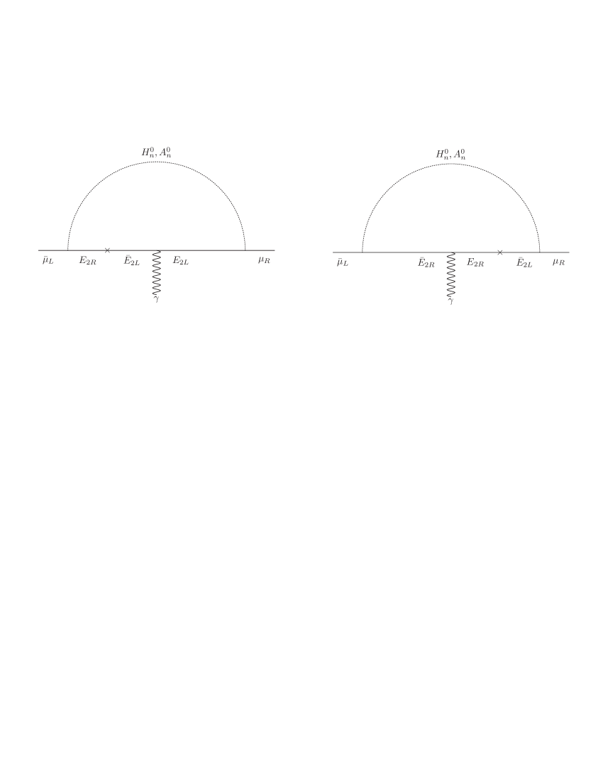
Figure 1: Models 1 and 2. One-loop Feynman diagram contributing to the charged lepton mass matrix. Here $i,j,k=1,2,3$.

III Scalar Potential

In this section we analyze the scalar potential of model 1. The scalar potential invariant under the symmetries of the model has the form:

$$V= -\mu_{\phi}^{2}(\phi^{\dagger}\phi)-\mu_{\eta}^{2}(\eta^{\dagger}\eta)-\mu_{\rho}^{2}(\rho^{\dagger}\rho)-\mu_{\xi}^{2}(\xi^{\dagger}\xi)-\mu_{\chi}^{2}(\chi^{\dagger}\chi)+\lambda_{1}(\phi^{\dagger}\phi)(\phi^{\dagger}\phi)+\lambda_{2}(\eta^{\dagger}\eta)(\eta^{\dagger}\eta)$$

$$+\lambda_{3}(\rho^{\dagger}\rho)(\rho^{\dagger}\rho)+\lambda_{4}(\xi^{\dagger}\xi)(\xi^{\dagger}\xi)+\lambda_{5}(\chi^{\dagger}\chi)(\chi^{\dagger}\chi)+\lambda_{6}(\phi^{\dagger}\eta)(\eta^{\dagger}\phi)+\lambda_{7}(\eta^{\dagger}\rho)(\rho^{\dagger}\eta)+\lambda_{8}(\eta^{\dagger}\eta)(\rho^{\dagger}\rho)$$

$$+\lambda_{9}(\phi^{\dagger}\xi)(\xi^{\dagger}\phi)+\lambda_{10}(\phi^{\dagger}\chi)(\chi^{\dagger}\phi)+\lambda_{11}(\phi^{\dagger}\phi)(\xi^{\dagger}\xi)+\lambda_{12}(\phi^{\dagger}\phi)(\chi^{\dagger}\chi)+\lambda_{13}(\xi^{\dagger}\xi)(\chi^{\dagger}\chi)$$

$$+\lambda_{14}(\xi^{\dagger}\chi)(\chi^{\dagger}\xi)+\lambda_{15}(\phi^{\dagger}\phi)(\eta^{\dagger}\eta)+\lambda_{16}(\phi^{\dagger}\phi)(\rho^{\dagger}\rho)+f(\eta^{\dagger}\phi\rho+\text{h.c})+\lambda_{17}(\eta^{\dagger}\chi)(\chi^{\dagger}\eta)$$

$$+\lambda_{18}(\rho^{\dagger}\chi)(\chi^{\dagger}\rho)+\lambda_{19}(\eta^{\dagger}\xi)(\xi^{\dagger}\eta)+\lambda_{20}(\rho^{\dagger}\xi)(\xi^{\dagger}\rho)+\lambda_{21}(\rho^{2}\xi\chi+\text{h.c})$$ (11)

where the $SU(2)_{L}$ scalar doublets are given by

$$\phi=\begin{pmatrix}\phi^{\pm}\\ \phi^{0}\end{pmatrix},\ \ \ \eta=\begin{pmatrix}\eta^{\pm}\\ \eta^{0}\end{pmatrix}$$ (12)

Here, $\phi$ is the SM Higgs doublet and $\eta$ is the inert $SU(2)$ scalar doublet. The coupling terms of $\phi S_{2}\eta$, $\eta\phi\sigma S_{2}$ and $S_{2}S_{1}\chi\xi$ are considered in the vertices of diagrams in Figure 2 and Figure 3 whereas in the scalar potential in Eq. (11) we consider the common terms in Model 1 and Model 2 to study phenomenological aspects like muon g-2 in Section V and dark matter in Section VI.

For finding constraints on the parameters $\lambda_{i}$ from the condition that the scalar potential $V$ is bounded from below, we just need to examine the quartic terms of the scalar potential as in BHATTACHARYYA_2016 . Here we considered quartic terms in the scalar potential that are relevant for $g-2$ and Dark Matter phenomenology. For convenience we define $a=\phi^{\dagger}\phi$, $b=\eta^{\dagger}\eta$, $c=\rho^{\dagger}\rho$, $d=\Re(\phi^{\dagger}\eta)$, $e=\Im(\phi^{\dagger}\eta)$, $g=\Re(\eta^{\dagger}\rho)$, $h=\Im(\eta^{\dagger}\rho)$, $z=\eta^{\dagger}\phi\rho$, $j=\Re(\eta^{\dagger}\chi)$, $k=\Im(\eta^{\dagger}\chi)$, $l=\Re(\rho^{\dagger}\chi)$, $m=\Im(\rho^{\dagger}\chi)$, $n=\Re(\eta^{\dagger}\xi)$, $p=\Im(\eta^{\dagger}\xi)$, $q=\Re(\rho^{\dagger}\xi)$, $r=\Im(\rho^{\dagger}\xi)$, $x=\rho^{2}\xi\chi$. With this notation we can write the quartic terms $V_{4}\subset V$ as

$$V_{4}= \left(\lambda_{1}^{1/2}a-\lambda_{2}^{1/2}b\right)^{2}+\left(\lambda_{2}^{1/2}b-\lambda_{3}^{1/2}c\right)^{2}+\left(\lambda_{15}+2\lambda_{1}^{1/2}\lambda_{2}^{1/2}\right)\left(ab-d^{2}-e^{2}\right)$$

$$+(\lambda_{8}+2(\lambda_{2}\lambda_{3})^{1/2})(bc-g^{2}-h^{2})+\left(\lambda_{8}+\lambda_{7}+2\left(\lambda_{2}\lambda_{3}\right)^{1/2}\right)\left(g^{2}+h^{2}\right)$$

$$+\left(\lambda_{15}+\lambda_{6}+2\left(\lambda_{1}\lambda_{2}\right)^{1/2}\right)\left(d^{2}+e^{2}\right)+\lambda_{16}(ac)+fz+\lambda_{17}(j^{2}+k^{2})$$

$$+\lambda_{18}(l^{2}+m^{2})+\lambda_{19}(n^{2}+p^{2})+\lambda_{20}(q^{2}+r^{2})+\lambda_{21}(x+\text{h.c.})$$

We require that there are no directions in the field space along which $V\to-\infty$. This leads to the following constraints on the $\lambda_{i}$:

• If $a=0$ then $d=e=z=0$, so we obtain $\lambda_{2}>0$

• If $b=0$ we obtain $\lambda_{1}>0$ and $\lambda_{3}>0$

• If $c=0$ and $ab=d^{2}+e^{2}$ we obtain $\lambda_{15}+2\sqrt{\lambda_{1}\lambda_{2}}>0$

• If $a=\sqrt{\lambda_{2}/\lambda_{1}}b$ and $g=h=d=e=0$ then $\lambda_{8}+2\sqrt{\lambda_{2}\lambda_{3}}>0$

• If $b=\sqrt{\lambda_{3}/\lambda_{2}}c$, $bc=g^{2}+h^{2}$ and $d=e=0$ then $\lambda_{8}+\lambda_{7}+2\sqrt{\lambda_{2}\lambda_{3}}>0$

• $\lambda_{15}+\lambda_{6}+2\sqrt{\lambda_{1}\lambda_{2}}>0$

These constraints are used in our numerical analysis of muon anomalous magnetic moment and dark matter.

Due to the scalar field charge assignments the mass matrix $M^{2}_{\eta\rho}$ is the same in both our Models 1 and 2, described in the previous sections. In the basis $\mathop{\mathrm{R}e}\eta^{0}$, $\mathop{\mathrm{R}e}\rho$, $\mathop{\mathrm{I}m}\eta^{0}$, $\mathop{\mathrm{I}m}\rho$ this matrix is given by:

$$M^{2}_{\eta\rho}=\left(\begin{array}[]{cccc}m_{11}&m_{12}&0&0\\ m_{21}&m_{22}&0&0\\ 0&0&m_{33}&m_{34}\\ 0&0&m_{43}&m_{44}\end{array}\right)$$ (17)

where the matrix entries are:

$$m_{11} =-\mu^{2}{}_{\eta}+\frac{1}{2}\lambda_{19}v_{\xi}^{2}+\frac{1}{2}\lambda_{17}v_{\chi}^{2}+\frac{1}{2}\lambda_{6}v_{\phi}^{2}+\frac{1}{2}\lambda_{15}v_{\phi}^{2},$$ (18)

$$m_{22} =-\mu^{2}{}_{\rho}+\lambda_{21}v_{\xi}v_{\chi}+\frac{1}{2}\lambda_{20}v_{\xi}^{2}+\frac{1}{2}\lambda_{18}v_{\chi}^{2}+\frac{1}{2}\lambda_{16}v_{\phi}^{2},$$ (19)

$$m_{33} =-\mu^{2}{}_{\eta}+\frac{1}{2}\lambda_{19}v_{\xi}^{2}+\frac{1}{2}\lambda_{17}v_{\chi}^{2}+\frac{1}{2}\lambda_{6}v_{\phi}^{2}+\frac{1}{2}\lambda_{15}v_{\phi}^{2},$$ (20)

$$m_{44} =-\mu^{2}{}_{\rho}-\lambda_{21}v_{\xi}v_{\chi}+\frac{1}{2}\lambda_{20}v_{\xi}^{2}+\frac{1}{2}\lambda_{18}v_{\chi}^{2}+\frac{1}{2}\lambda_{16}v_{\phi}^{2},$$ (21)

$$m_{12} =m_{21}=\frac{fv_{\phi}}{\sqrt{2}},$$ (22)

$$m_{34} =m_{43}=-\frac{fv_{\phi}}{\sqrt{2}}\,.$$ (23)

The upper left and lower right blocks of the matrix given in Eq. (17) correspond to the squared scalar mass matrices for the dark CP even and CP odd scalars, respectively. Their diagonalization yields the following physical CP even and CP odd mass eigenstates defined as follows:

$$\left(\begin{array}[]{c}H_{1}\\ H_{2}\end{array}\right)=\left(\begin{array}[]{cc}\cos\theta_{H}&\sin\theta_{H}\\ -\sin\theta_{H}&\cos\theta_{H}\end{array}\right)\left(\begin{array}[]{c}\eta_{R}\\ \rho_{R}\end{array}\right),\hskip 28.45274pt\left(\begin{array}[]{c}A_{1}\\ A_{2}\end{array}\right)=\left(\begin{array}[]{cc}\cos\theta_{A}&\sin\theta_{A}\\ -\sin\theta_{A}&\cos\theta_{A}\end{array}\right)\left(\begin{array}[]{c}\eta_{I}\\ \rho_{I}\end{array}\right).$$ (24)

These relations will be used in the analysis of the lepton mass generation, muon anomalous magnetic moment and dark matter we will carry out in the following sections.

IV Lepton sector masses

Here we show that, both above specified one- and two-loop models offer radiative mechanisms for the generation of charged lepton and neutrino masses. In both models the charged lepton masses are generated at one-loop level, according to Fig. 1. On the other hand, neutrino masses arise at one- and two-loop levels depending on the model, as shown in Figs. 2, 3.

IV.1 Charged lepton masses

From the SM charged lepton Yukawa terms in (II.1) and (II.2), we find that the mass matrix for SM charged leptons in models 1 and 2 is represented by the diagram in Fig. 1. Analytically we have

$$\left(M_{l}\right)_{ij}=\sum_{k=1}^{3}\frac{y_{ik}^{\left(E\right)}x_{kj}^{\left(l\right)}m_{E_{k}}}{16\pi^{2}}\left\{\left[F\left(m_{H_{1}}^{2},m_{E_{k}}^{2}\right)-F\left(m_{H_{2}}^{2},m_{E_{k}}^{2}\right)\right]\sin 2\theta_{H}-\left[F\left(m_{A_{1}}^{2},m_{E_{k}}^{2}\right)-F\left(m_{A_{2}}^{2},m_{E_{k}}^{2}\right)\right]\sin 2\theta_{A}\right\},$$ (25)

where $F\left(m_{1}^{2},m_{2}^{2}\right)$ is the function defined as,

$$F\left(m_{1}^{2},m_{2}^{2}\right)=\frac{m_{1}^{2}}{m_{1}^{2}-m_{2}^{2}}\ln\left(\frac{m_{1}^{2}}{m_{2}^{2}}\right).$$ (26)

$m_{H_{1}}$ and $m_{H_{2}}$ are the masses of the physical CP even scalars, whereas $m_{A_{1}}$ and $m_{A_{2}}$ are those of the inert pseudoscalars.

The SM charged lepton mass matrix can be parametrized as follows:

$$M_{l} = A_{l}J_{E}^{-1}B_{l}^{T},\hskip 19.91684pt\hskip 19.91684ptJ_{E}=\left(\begin{array}[]{ccc}\frac{1}{16\pi^{2}}m_{E_{1}}K_{E}^{\left(1\right)}&0&0\\ 0&\frac{1}{16\pi^{2}}m_{E_{2}}K_{E}^{\left(2\right)}&0\\ 0&0&\frac{1}{16\pi^{2}}m_{E_{3}}K_{E}^{\left(3\right)}\end{array}\right),$$ (30)

where:

$$K_{E}^{\left(n\right)} = \left[F\left(m_{H_{1}}^{2},m_{E_{n}}^{2}\right)-F\left(m_{H_{2}}^{2},m_{E_{n}}^{2}\right)\right]\sin 2\theta_{H}-\left[F\left(m_{A_{1}}^{2},m_{E_{n}}^{2}\right)-F\left(m_{A_{2}}^{2},m_{E_{n}}^{2}\right)\right]\sin 2\theta_{A},\hskip 14.22636ptn=1,2,3$$

$$A_{l} = V_{L}^{\left(l\right)}\widetilde{M}_{l}^{\frac{1}{2}}J_{E}^{\frac{1}{2}},\hskip 19.91684pt\hskip 19.91684ptB_{l}=V_{R}^{\left(l\right)}\widetilde{M}_{l}^{\frac{1}{2}}J_{E}^{\frac{1}{2}},\hskip 19.91684pt\hskip 19.91684pt\widetilde{M}_{l}=\left(\begin{array}[]{ccc}m_{e}&0&0\\ 0&m_{\mu}&0\\ 0&0&m_{\tau}\end{array}\right)$$ (34)

Thus, both models have enough parametric freedom to successfully accommodate the SM charged lepton masses. Despite the fact that the all SM charged lepton masses arise at one loop level, the hierarchy between such masses can be successfully accommodated by having some moderate hierarchy as well as a deviation from the scenario of universality of the charged lepton Yukawa couplings. It is worth mentioning that since the SM charged lepton mass matrix arises at one loop level, the effective charged lepton Yukawa couplings are proportional to a product of two other dimensionless couplings, thus implying that a moderate hierarchy in those couplings can give rise to a quadratically larger hierarchy in the effective couplings.

IV.2 Neutrino mass matrix

From the neutrino Yukawa interactions of both radiative models described above, we find the following neutrino mass terms:

$$-\mathcal{L}_{mass}^{\left(\nu\right)}=\frac{1}{2}\left(\begin{array}[]{ccc}\overline{\nu_{L}^{C}}&\overline{\nu_{R}}&\overline{N_{R}}\end{array}\right)M_{\nu}\left(\begin{array}[]{c}\nu_{L}\\ \nu_{R}^{C}\\ N_{R}^{C}\end{array}\right)+H.c.=\varepsilon\,\overline{\nu_{L}}\nu_{R}+m\,\overline{\nu_{L}}N_{R}+M\,\overline{\nu_{R}^{C}}N_{R}+H.c.$$ (35)

where neutrino mass matrix $M_{\nu}$ is given by Eq. (1), after which we also specified lepton number assignment of the neutrino sector. As seen, the only source of lepton number violation is the $m$-term. In our models this submatrix is generated after spontaneous breaking of the electroweak symmetry by a VEV $\langle\phi^{0}\rangle=v$ of the SM Higgs doublet $\phi$, which also breaks $U(1)_{L}$ of lepton number symmetry of both models with the charge assignments $L(\nu_{L})=L(\nu_{R})=-L(N_{R})=L(\phi)/2=L(\eta)/2=1$. Therefore, as seen from Eqs. (II.1) and (II.2) we have

$$m_{in}=y_{in}^{\left(N\right)}\frac{v}{\sqrt{2}},\hskip 19.91684pt\hskip 19.91684pti=1,2,3,\hskip 19.91684pt\hskip 19.91684ptn=1,2.$$ (36)

Since the global $U(1)_{L}$ is spontaneously broken by $\langle\phi^{0}\rangle$, one typically expects appearance of the corresponding SM-non-sterile massless Majoron, which is phenomenologically unacceptable. Fortunately, it does not appear as a physical state. The simultaneous spontaneous breaking the SM gauge symmetry and $U(1)_{L}$ guaranties that the Majoron coincides with the electrically neutral CP-odd would-be-Goldstone absorbed by $Z$-boson. The Dirac submatrix $\varepsilon$ is generated at one and two loops in the models of sections II.1 and II.2, respectively. The corresponding Feynman diagram are shown in Figs. 2 and 3.

The submatrix $\varepsilon$ takes the form:

$$\varepsilon_{in}\simeq\left\{\begin{array}[]{l}\mathop{\displaystyle\sum}\limits_{j=1}^{3}\mathop{\displaystyle\sum}\limits_{k=1}^{3}\frac{y_{ik}^{\left(E\right)}x_{kn}^{\left(\nu\right)}m_{E_{k}}}{16\pi^{2}}\left(R_{C}\right)_{1j}\left(R_{C}\right)_{2j}F\left(m_{H_{j}^{\pm}}^{2},m_{E_{k}}^{2}\right),\hskip 14.22636pt\mbox{for the one loop model}\\ \\ \mathop{\displaystyle\sum}\limits_{k=1}^{2}\frac{\lambda vR_{1k}R_{2k}J\left(\frac{m_{\sigma}^{2}}{m_{H_{k}^{\pm}}^{2}}\right)}{96\pi^{2}m_{S}^{2}}\times\\ \times\left[y^{\left(E\right)}M_{E}\left(x^{\left(E\right)}\right)^{{\dagger}}M_{\widetilde{E}}^{T}\left(x^{\left(\nu\right)}\right)^{T}+\left(x^{\left(\nu\right)}\right)M_{\widetilde{E}}\left(x^{\left(E\right)}\right)^{\ast}\left(M_{E}\right)^{T}\left(y^{\left(E\right)}\right)^{T}\right],\hskip 5.69046pt\mbox{for the 2 loop model}.\end{array}\right.$$ (37)

where, for the two loop model, we have set $m_{S}=\max\left(m_{\eta^{\pm}},m_{H_{k}^{\pm}},m_{\sigma}\right)$ and we have assumed $m_{\eta^{\pm}}\simeq m_{H_{1}^{\pm}}\simeq m_{H_{2}^{\pm}}$ and $m_{E_{i}}$, $m_{\widetilde{E}_{i}}<<m_{\eta^{\pm}}$, $m_{H_{k}^{\pm}}<<$ $m_{\sigma}$ ($i=1,2,3$). Besides that, $\lambda$ stands for the quartic scalar coupling associated with the interaction $\varepsilon_{ab}\left(\eta^{\ast}\right)^{a}\left(\phi^{\ast}\right)^{b}S_{2}^{+}\sigma^{\ast}+h.c$. Furthermore, under the aforementioned assumptions, the loop function for the two loop model takes the form Herrero-Garcia:2014hfa ; McDonald:2003zj :

$$J\left(\varkappa\right)=\left\{\begin{array}[]{l}1+\frac{3}{\pi^{2}}\left(\ln^{2}\varkappa-1\right),\hskip 5.69046pt\text{for}\hskip 5.69046pt\varkappa>>1\\ \\ 1,\hskip 5.69046pt\text{for}\hskip 5.69046pt\varkappa\rightarrow 0.\end{array}\right.,$$

and the electrically charged scalars in the interaction and physical basis are related as:

$$\left(\begin{array}[]{c}\eta^{\pm}\\ S_{1}^{\pm}\\ S_{2}^{\pm}\end{array}\right) = R_{C}\left(\begin{array}[]{c}H_{1}^{\pm}\\ H_{2}^{\pm}\\ H_{3}^{\pm}\end{array}\right),\hskip 28.45274pt\mbox{for the one loop model},$$ (44)

$$\left(\begin{array}[]{c}S_{1}^{\pm}\\ S_{2}^{\pm}\end{array}\right) = R\left(\begin{array}[]{c}H_{1}^{\pm}\\ H_{2}^{\pm}\end{array}\right)=\left(\begin{array}[]{cc}\cos\theta&-\sin\theta\\ \sin\theta&\cos\theta\end{array}\right)\left(\begin{array}[]{c}H_{1}^{\pm}\\ H_{2}^{\pm}\end{array}\right),\hskip 28.45274pt\eta^{\pm}=H^{\pm},\hskip 28.45274pt\mbox{for the two loop model},$$ (53)

where $R_{C}$ is a real orthogonal $3\times 3$ matrix.

Figure 2: Model 1. One-loop Feynman diagram contributing to the neutrino mass submatrix $\varepsilon$. Here $i,k,r=1,2,3$, $n=1,2$.

Figure 3: Model 2. Two-loop Feynman diagram contributing to the neutrino mass submatrix $\varepsilon$. Here $i,k,r=1,2,3$, $n=1,2$.

From the linear seesaw mass matrix (1), (35) we have the physical neutrino mass matrices

$$M_{\nu}^{\left(1\right)} \cong -\left[\varepsilon M^{-1}m^{T}+m\left(M^{T}\right)^{-1}\varepsilon^{T}\right],$$ (54)

$$M_{\nu}^{\left(2\right)} \cong -\frac{1}{2}\left(M+M^{T}\right)\left[1_{2\times 2}-\left(M+M^{T}\right)^{-2}m_{1}^{T}m_{1}\right]-\left(M+M^{T}\right)^{-1}m_{1}^{T}m_{1},\hskip 19.91684pt\hskip 19.91684ptm_{1}=m-\varepsilon,$$ (55)

$$M_{\nu}^{\left(3\right)} \cong \frac{1}{2}\left(M+M^{T}\right)\left[1_{2\times 2}-\left(M+M^{T}\right)^{-2}m_{2}^{T}m_{2}\right]+\left(M+M^{T}\right)^{-1}m_{2}^{T}m_{2},\hskip 19.91684pt\hskip 19.91684ptm_{2}=m+\varepsilon,$$ (56)

where $M_{\nu}^{\left(1\right)}$ corresponds to the active neutrino mass matrix whereas $M_{\nu}^{\left(2\right)}$ and $M_{\nu}^{\left(3\right)}$ are the sterile neutrino mass matrices. The physical neutrino spectrum is composed of 3 light active neutrinos and 2 pairs of nearly degenerate sterile exotic pseudo-Dirac neutrinos $N^{\pm}_{1}$ and $N^{\pm}_{2}$. For more details about diagonalization see Appendix A.

Assuming that the scalar and fermionic seesaw mediators in the diagrams Figs. 2 and 3 have masses at the scales $m_{S}$ and $m_{E}$, respectively, the light active neutrino mass scale can be estimated for the one and two loop models as follows:

$$m_{\nu}\sim\left\{\begin{array}[]{l}\frac{\lambda y^{3}v^{2}fm_{E}}{16\pi^{2}m_{S}^{2}M}\hskip 14.22636pt\mbox{for the one loop model}\\ \\ \frac{\lambda^{2}y^{4}v^{2}m_{E}^{2}}{256\pi^{4}m_{S}^{2}M}\hskip 14.22636pt\mbox{for the two loop model}.\end{array}\right.$$ (57)

where $y$ is a common coupling of the neutrino Yukawa interactions, whereas $\lambda$ is the couplings of the quartic scalar interaction $S_{1}^{+}S_{2}^{-}\chi\xi$, whereas $f$ is the trilinear scalar coupling for the interaction $\eta^{\dagger}\phi\rho$ (see Figures 2 and 3). Assuming that $y\sim\lambda\sim\mathcal{O}(0.1)$, $f\sim m_{E}\sim\mathcal{O}(1)$ TeV, $m_{S}\sim\mathcal{O}(10)$ TeV, we find from Eq. (57) that the light active neutrino mass scale $m_{\nu}\sim 50$ meV can be reproduced in the one loop linear seesaw model provided that the mass scale of the heavy pseudo-Dirac neutrinos satisfies $M\sim\mathcal{O}(10^{3})$ TeV. Regarding the two loop linear seesaw model, the choice $\lambda\sim\mathcal{O}(1)$, $y\sim\mathcal{O}(0.1)$, $f\sim m_{E}\sim\mathcal{O}(1)$ TeV, $m_{S}\sim\mathcal{O}(10)$ TeV allows us to reproduce the light active neutrino mass scale $m_{\nu}\sim 50$ meV, for pseudo-Dirac neutrinos with masses around $M\sim\mathcal{O}(1)$ TeV.

V $g-2$ muon anomaly

Figure 4: Loop Feynman diagrams contributing to the muon anomalous magnetic moment. Here $n=1,2$.

The current experimental data on the anomalous dipole magnetic moment of the muon $a_{\mu}=(g_{\mu}-2)/2$ show significant deviation from its SM value

$$\Delta a_{\mu} = a_{\mu}^{\mathrm{exp}}-a_{\mu}^{\mathrm{SM}}=\left(2.49\pm 0.48\right)\times 10^{-9}\hskip 48.36967pt\mbox{\cite[cite]{\@@bibref{Authors Phrase1YearPhrase2}{Hagiwara:2011af,Davier:2017zfy,Blum:2018mom,Keshavarzi:2018mgv,Aoyama:2020ynm,Muong-2:2023cdq}{\@@citephrase{(}}{\@@citephrase{)}}}}$$ (58)

In our models this deviation is given by the sum of the partial contributions:

$$\Delta a_{\mu}=\mathop{\displaystyle\sum}\limits_{i=1}^{2}\mathop{\displaystyle\sum}\limits_{\Phi=H^{0}_{i},A^{0}_{i}}\Delta a_{\mu}(\Phi),$$ (59)

shown in Fig. 4. The analytical form for the neutral scalar and pseudoscalar contributions at one loop to $\Delta a_{\mu}$ can be found in Diaz:2002uk ; Jegerlehner:2009ry ; Kelso:2014qka ; Lindner:2016bgg ; Kowalska:2017iqv . Using these results we write the contributions of the neutral scalars $\Phi=H_{i},A^{0}_{i}$ ($i=1,2$) defined in Eq. (24). These contributions are given by:

$$\Delta a_{\mu}=\frac{m_{\mu}^{2}}{8\pi^{2}}\left\{\mathop{\displaystyle\sum}\limits_{i=1}^{2}\omega_{S\mu}^{2}\frac{G_{S}^{\left(\mu\right)}\left(m_{E_{2}},m_{H_{i}}\right)}{m_{H_{i}}^{2}}+\mathop{\displaystyle\sum}\limits_{i=1}^{2}\omega_{P\mu}^{2}\frac{G_{P}^{\left(\mu\right)}\left(m_{E_{2}},m_{A_{i}^{0}}\right)}{m_{A_{i}^{0}}^{2}}\right\}$$ (60)

where the loop function is given by:

$$G_{S,P}^{(l)}(m_{E},m_{\Phi})=\int_{0}^{1}dx\frac{x^{2}(1-x\pm\epsilon_{lE})}{(1-x)(1-x\lambda_{\mu\Phi}^{2})+x\epsilon_{\mu E}^{2}\lambda_{\mu\Phi}^{2}},\hskip 28.45274pt\Phi=H^{0},A^{0}$$ (61)

with $\lambda_{\mu\Phi}=m_{\mu}/m_{\Phi}$, $\epsilon_{\mu E}=m_{E_{2}}/m_{\mu}$. In the loop function $G_{S,P}(\Phi)$, the plus and minus signs stand for the scalar (CP-even) and pseudoscalar (CP-odd) contributions, respectively. The quantities $\omega_{S\mu}$ $\omega_{P\mu}$ are the effective Yukawa couplings for the interactions of the CP-even and CP-odd scalar fields with fermions in the form $\overline{l}_{iL}\eta E_{jR}$ and $\overline{E}_{iL}\rho l_{jR}$ after diagonalization.

The central experimental value the muon anomalous magnetic moment shown in Eq. (58) can be successfully reproduced at the following benchmark point specified in terms of the masses of the scalars $A^{0}_{i},H_{k}$ and charged exotic leptons $E_{n}$ along with the effective Yukawa couplings $\omega_{S\mu(P\mu)}$:

$$m_{H_{1}} \approx 10164.1\,\text{GeV} m_{H_{2}} \approx 3782.1\,\text{GeV} m_{A^{0}_{1}} \approx 5860.1\,\text{GeV}$$ (62)

$$m_{A^{0}_{2}} \approx 3781.9\,\text{GeV} m_{E_{1}} \approx 611.5\,\text{GeV} m_{E_{2}} \approx 625\,\text{GeV}$$ (63)

$$\omega_{S\mu} \approx 1.569 \omega_{P\mu} \approx 1.578$$ (64)

According to Eqs. (18)-(23), this benchmark point corresponds to the model parameters

$$v_{\phi} =246\,\text{GeV}, v_{\chi} \approx 8381.8\,\text{ GeV}\,\ v_{\xi} \approx 8381.8\ ,\text{GeV}$$ (65)

$$\mu_{\rho} \approx 383.5\,\text{GeV}\, \mu_{\eta} \approx 383.5\,\text{GeV}\, f \approx 830\,\text{GeV}$$ (66)

$$\lambda_{6} =\lambda_{15}=\lambda_{16}\approx 0.0970 \lambda_{17} =\lambda_{19}\approx 0.205 \lambda_{18} =\lambda_{20}=\lambda_{21}\approx 0.981$$ (67)

VI Scalar Dark Matter

As we already mentioned, a viable DM candidate in the one loop radiative linear seesaw model is the lightest among the $\widetilde{Z}_{2}$-odd scalars. Regarding the two loop linear seesaw model, due to the preserved $Z_{2}^{(2)}\times\widetilde{Z}_{2}$ symmetry, one scalar DM candidate is the lightest among the Re $\sigma$ and Im $\sigma$ and the other one is the lightest among $\widetilde{Z}_{2}$-odd scalars. This implies that in this model we have a multicomponent dark matter and thus the resulting relic density will be the sum of the relic densities generated by these two scalar DM candidates. As to a fermionic DM candidate, this could be the lightest of the $\widetilde{Z}_{2}$-odd mass eigenstate linear combinations of $\nu_{nR}$, $N_{nR}$ ($n=1,2$) with the typical mass $M$ specified in Eqs. (55), (56). However, it is less interesting DM candidate. In fact, as we showed in sec. IV.2, the smallness of the active neutrino masses in Eq. (57) implies $M$ to be sufficiently large. Otherwise Yukawa and quartic couplings are very small making the related phenomenology scarce, such as for example very tiny rates for charged lepton flavor violating decays. On the other hand the $\widetilde{Z}_{2}$-odd right handed neutrino states with $M$ greater than the SM Higgs boson mass $M_{H}$ are not DM candidates since they can decay into the SM Higgs boson and an active neutrino.

For these reasons we focus on the scalar DM candidates and proceed to analyze the implications of the one loop linear seesaw model in dark matter. The detailed study of the implications of the two loop linear seesaw model in dark matter is left beyond the scope of the present paper and is deferred for a future work. In the benchmark scenario (62)-(67) the DM candidate is the CP-odd scalar $A^{0}_{2}$, defined in Eq. (24). We denote this particle as $A$. After diagonalizing the CP-odd scalar mass matrix in Eq. (17), we find the couplings of $A$ to the $126$ GeV SM-like Higgs boson

$$\lambda_{hhAA}= \lambda_{16}\sin^{2}\theta_{A}+\lambda_{6}\cos^{2}\theta_{A}+\lambda_{15}\cos^{2}\theta_{A}$$ (68)

$$\lambda_{hAA}= -\sqrt{2}f\sin\theta_{A}\cos\theta_{A}+\lambda_{16}v_{\phi}\sin^{2}\theta_{A}+\lambda_{6}v_{\phi}\cos^{2}\theta_{A}$$

$$+\lambda_{15}v_{\phi}\cos^{2}\theta_{A},$$ (69)

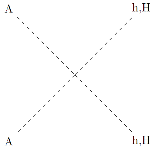
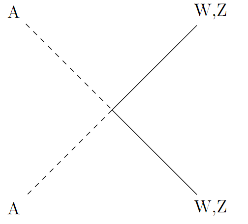
where, $\theta_{A}\approx 3.13$ is the mixing angle of the CP-odd scalar fields that was fitted with muon g-2 anomaly in Section V. As in our scenario the dark matter candidate is a scalar $A$, it can mainly annihilate into a pair of SM Higgses and into a pair of the SM electroweak bosons as shown in the Feynman diagrams in Fig. 5.

Figure 5: Relevant Feynman diagrams for DM annihilation

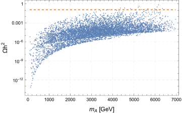
Having this at hand, we calculated DM relic abundance $\Omega h^{2}$ with the help of micrOMEGAs5.2 B_langer_2018 and generated a scatter plot characterizing the correlation between $\Omega h^{2}$ and DM candidate mass $m_{A}$, shown in Fig. 6 for the case of the benchmark point (62)-(67).

Figure 6: Correlation plot of the relic abundance $\Omega h^{2}$ as a function of the DM candidate mass $m_{A}$. The orange doted line is the experimental limit for Dark Matter relic abundance.

The plot in Fig. 6 shows that the relic abundance is near the observed value $\Omega h^{2}=0.12\pm 0.0012$ Planck2020 for masses above $4000$ GeV, and only few points are excluded by the limit. Every point in this plot fits $g-2$ muon anomaly. The best fit value gives $\Omega h^{2}=0.1231$ and $\Delta a_{\mu}=2.79\times 10^{-9}$ are inside the $3\sigma$ and $1\sigma$ experimentally allowed ranges, respectively. With the restrictions given by the DM relic abundance, we have numerically checked that the obtained values for the spin independent cross section are two orders of magnitude lower than the most recent bounds imposed by the Xenon1T experiment.

VII Charged Lepton Flavor Violation

In this section we analyze charged lepton flavor violation (cLFV) processes present due to the mixing between active and heavy sterile neutrinos. Here we focus on $l_{i}\rightarrow l_{j}\gamma$ decay. At one loop level its branching ratio is Langacker:1988up ; Lavoura:2003xp ; Hue:2017lak

$$\text{BR}\left(l_{i}\rightarrow l_{j}\gamma\right) = \frac{\alpha_{W}^{3}s_{W}^{2}m_{l_{i}}^{5}}{256\pi^{2}m_{W}^{4}\Gamma_{i}}\left|G_{ij}\right|^{2}$$ (70)

$$G_{ij} \simeq \sum_{k=1}^{3}\left(\left[\left(1-RR^{\dagger}\right)U_{\nu}\right]^{\ast}\right)_{ik}\left(\left(1-RR^{\dagger}\right)U_{\nu}\right)_{jk}G_{\gamma}\left(\frac{m_{\nu_{k}}^{2}}{m_{W}^{2}}\right)+2\sum_{l=1}^{2}\left(R^{\ast}\right)_{il}\left(R\right)_{jl}G_{\gamma}\left(\frac{m_{N_{R_{l}}}^{2}}{m_{W}^{2}}\right),$$ (71)

$$G_{\gamma}(x) = \frac{10-43x+78x^{2}-49x^{3}+18x^{3}\ln x+4x^{4}}{12\left(1-x\right)^{4}},$$

where $\Gamma_{\mu}=3\times 10^{-19}$ GeV is the total muon decay width, $U_{\nu}$ is the matrix that diagonalizes the light neutrino mass matrix which, in our case, is equal to the Pontecorvo-Maki-Nakagawa-Sakata (PMNS) matrix since the charged lepton mixing matrix is set to be equal to the identity $U_{\ell}=\mathbb{I}$. In addition, the matrix $R$ is given by

$$R=\frac{1}{\sqrt{2}}mM^{-1},$$ (72)

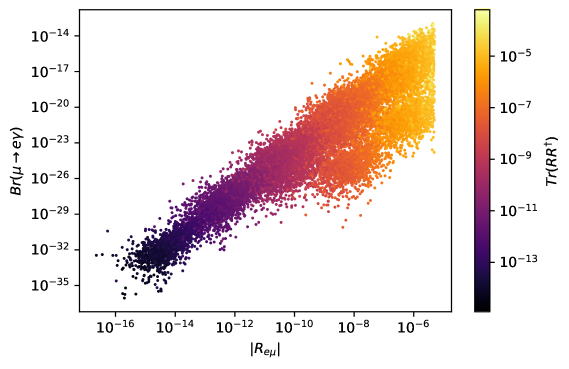
where $M$ and $m$ are $2\times 2$ and $3\times 2$ entries of $7\times 7$ neutrino mass matrix in Eq. (1), respectively. In Fig. 7 we plot the values of the branching ratio Br($\mu\rightarrow e\gamma$) as a function of $\left|R_{e\mu}\right|$ for different values of Tr$[RR^{\dagger}]$.

Figure 7: $\mu\rightarrow e\gamma$ branching ratio as a function of $|R_{e\mu}|$. The color surface is the value of Tr$[RR^{\dagger}]$.

The points have been generated for the benchmark scenario (62)-(67) by randomly varying the neutrino mass matrix parameters (35) in the ranges $m\in[10^{-3},10^{-1}]$GeV, $M\in[10,10^{3}]$GeV. According to Sec. IV.2 these points are compatible with the active neutrino mass scales $m_{\nu}\sim 50$ meV. Fig. 7 shows that there are large number of the model points below the experimental upper bound $Br(\mu\rightarrow e\gamma)<4.2\times 10^{-13}$ many of which should be accessible in the future experiments.

VIII Leptogenesis

Here we analyze the implications of our two-loop model for leptogenesis. We skip the one-loop model, where the Yukawa couplings responsible of the neutrino mass, discussed in Sec. IV.2, are typically smaller than in the two-loop model and, as a result, its effect on leptogenesis should be smaller. To simplify our analysis we assume that $M$ is a diagonal matrix satisfying the condition $\left|M_{11}\right|\ll\left|M_{22}\right|$. In this case the Baryon asymmetry of the Universe (BAU) is dominated in our model by $N_{1}^{\pm}$ pseudo-Dirac sterile neutrino, defined in Sec. IV.2. We further assume that the exotic leptonic fields $E_{nR}$ and $\Omega_{nR}$ are heavier than the lightest pseudo-Dirac fermion $N_{1}^{\pm}=N_{\pm}$. We use the basis where the SM charged lepton mass matrix is diagonal. Then, the lepton asymmetry parameter, which is induced by the decay of $N_{\pm}$, has the following form Gu:2010xc ; Pilaftsis:1997jf :

$$\epsilon_{\pm}=\frac{\mathop{\displaystyle\sum}\limits_{i=1}^{3}\left[\Gamma\left(N_{\pm}\rightarrow\widetilde{E}_{i}S_{1}^{+}\right)-\Gamma\left(N_{\pm}\rightarrow\overline{\widetilde{E}}_{i}S_{1}^{-}\right)\right]}{\mathop{\displaystyle\sum}\limits_{i=1}^{3}\left[\Gamma\left(N_{\pm}\rightarrow\widetilde{E}_{i}S_{1}^{+}\right)+\Gamma\left(N_{\pm}\rightarrow\overline{\widetilde{E}}_{i}S_{1}^{-}\right)\right]}\simeq\frac{\mathop{\mathrm{I}m}\left\{\left(\left[\left(y_{N_{+}}\right)^{\dagger}\left(y_{N_{-}}\right)\right]^{2}\right)_{11}\right\}}{8\pi A_{\pm}}\frac{r}{r^{2}+\frac{\Gamma_{\pm}^{2}}{m_{N_{\pm}}^{2}}},$$ (73)

with:

$$r = \frac{m_{N_{+}}^{2}-m_{N_{-}}^{2}}{m_{N_{+}}m_{N_{-}}},\hskip 19.91684pt\hskip 19.91684ptA_{\pm}=\left[\left(y_{N_{\pm}}\right)^{\dagger}y_{N_{\pm}}\right]_{11},\hskip 19.91684pt\hskip 19.91684pt\Gamma_{\pm}=\frac{A_{\pm}m_{N_{\pm}}}{8\pi},$$

$$y_{N_{+}} = \frac{x^{\left(\nu\right)}}{\sqrt{2}}\left(1_{2\times 2}-\frac{1}{2}B_{2}^{T}B_{2}-B_{1}^{T}B_{2}\right),$$

$$y_{N_{-}} = \frac{x^{\left(\nu\right)}}{\sqrt{2}}\left(1_{2\times 2}-\frac{1}{2}B_{1}^{T}B_{1}\right),$$ (74)

$$B_{1} \simeq -\sqrt{2}m_{2}\left(M+M^{T}\right)^{-1}\simeq-\frac{1}{\sqrt{2}}m_{2}M^{-1}=-\frac{1}{\sqrt{2}}\left(m-\varepsilon\right)M^{-1},$$

$$B_{2} \simeq -\sqrt{2}m_{1}\left(M+M^{T}\right)^{-1}\simeq-\frac{1}{\sqrt{2}}m_{1}M^{-1}=-\frac{1}{\sqrt{2}}\left(m+\varepsilon\right)M^{-1}.$$

As mentioned in Dolan:2018qpy , neglecting the interference terms involving the two different sterile neutrinos $N_{\pm}$ leads to huge values of the washout parameter $K_{N^{+}}+K_{N^{-}}$. Thus, this effect must be taken into account. The small mass splitting in the pair of the states $N_{\pm}$, forming a pseudo-Dirac neutrino, leads to destructive interference in the scattering process Blanchet:2009kk properly reducing the washout parameter. Its effective value, including the interference term, is given by

$$K^{eff}\simeq\left(K_{N^{+}}\delta_{+}^{2}+K_{N^{-}}\delta_{-}^{2}\right),$$ (75)

where:

$$\delta_{\pm}=\frac{m_{N^{+}}-m_{N^{-}}}{\Gamma_{N^{\pm}}},\hskip 19.91684pt\hskip 19.91684ptK_{N^{\pm}}=\frac{\Gamma_{\pm}}{H\left(T\right)},\hskip 19.91684pt\hskip 19.91684ptH(T)=\sqrt{\frac{4\pi^{3}g^{\ast}}{45}}\frac{T^{2}}{M_{P}}$$ (76)

where $g^{\ast}=106.75$ is the number of effective relativistic degrees of freedom, $M_{Pl}=1.2\times 10^{9}$ GeV is the Planck constant and $T=m_{N_{\pm}}$. In the weak and strong washout regimes, the baryon asymmetry is related to the lepton asymmetry Pilaftsis:1997jf as follows

$$Y_{\Delta B} = \frac{n_{B}-\overline{n}_{B}}{s}=-\frac{28}{79}\frac{\epsilon_{+}+\epsilon_{-}}{g^{\ast}},\hskip 14.22636pt\text{for}\hskip 14.22636ptK^{eff}\ll 1,$$ (77)

$$Y_{\Delta B} = \frac{n_{B}-\overline{n}_{B}}{s}=-\frac{28}{79}\frac{0.3\left(\epsilon_{+}+\epsilon_{-}\right)}{g^{\ast}K^{eff}\left(\ln K^{eff}\right)^{0.6}},\hskip 14.22636pt\text{for}\hskip 14.22636ptK^{eff}\gg 1,$$ (78)

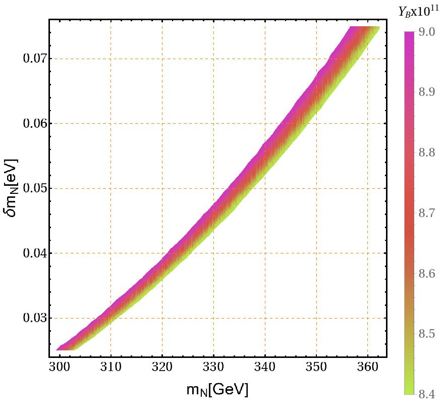
The correlation of the sterile neutrino mass splitting $\delta m_{N}$ with the mass of the lightest sterile neutrino for the weak washout regime is shown in Figure 8. To generate this plot, we performed a random scan in the ranges $\left(m_{\nu D}\right)_{ij}\in[1,150]$ GeV, $M_{11}\in[150,500]$ GeV, $M_{22}\in[1,2]$ TeV and $\delta m_{N}\in[0.5,1.5]$ eV. As indicated by Figure 8, an increase of the sterile neutrino mass splitting $\delta m_{N}$ yields larger values for the mass $m_{N}$ of the lightest pseudo-Dirac lepton, in order to successfully reproduce the observed value of the baryon asymmetry Planck:2018vyg

$$Y_{\Delta B}=\frac{n_{B}-n_{\bar{B}}}{s}=\left(0.87\pm 0.01\right)\times 10^{-10}$$ (79)

Such larger values of the lightest pseudo-Dirac lepton mass $m_{N}$ will give rise to smaller active-sterile neutrino mixing angles, thus yielding smaller rates for charged lepton flavor violating decays such as $\mu\to e\gamma$. As shown by Figure 8, our model is capable of successfully accommodating the baryon asymmmetry of the Universe via resonant leptogenesis.

Figure 8: Correlation of the sterile neutrino mass splitting $\delta m_{N}$ with the mass of the lighest sterile neutrino for the weak washout regime.

IX Conclusions

We have proposed two models where the tiny masses of the light active neutrinos are generated from a radiative linear seesaw mechanism, with the Dirac neutrino mass submatrix arising at one and two loop levels in the first and second model, respectively, due to the virtual electrically charged scalars and vector-like leptons running inside the loops. In these models, the masses of the SM charged leptons are generated from a one loop radiative seesaw mechanism, mediated by charged exotic vector like leptons and electrically neutral scalars. This loop pattern, engendering small masses to the light active neutrinos and the SM charged lepton masses, is ensured by a preserved $\widetilde{Z}_{2}$ discrete symmetry, which also guarantees stability of the scalar dark matter candidate in our models. These models can be treated as extended Inert Doublet Models (IDM), where the scalar content is augmented with the inclusion of several electrically neutral and electrically charged scalar singlets, whereas the lepton sector is enlarged with right handed Majorana neutrinos and charged exotic vector like leptons. We have found that these models can successfully comply with the constraints arising from charged lepton flavor violation, leptogenesis, dark matter and muon anomalous magnetic moment.

Comment

Our friend and collaborator Iván Schmidt passed away during the completion of this work. He will be sorely missed.

Appendix A Diagonalization of the neutrino mass matrix.

Here, for the convenience of the reader, we show in full detail the perturbative diagonalization procedure of the full $7\times 7$ neutrino mass matrix $M_{\nu}$ of Eq. (1). The elements of the submatrices $\varepsilon$, $m$ and $M$ obey the following hierarchy:

$$\varepsilon_{in}<<m_{in}<<M_{np},\hskip 19.91684pt\hskip 19.91684pti=1,2,3,\hskip 19.91684pt\hskip 19.91684ptn,p=1,2.$$ (80)

We start by applying the following first orthogonal transformation to the matrix $M_{\nu}$:

$$S_{\nu}^{T}M_{\nu}S_{\nu} = \left(\begin{array}[]{ccc}1_{3\times 3}&0_{3\times 2}&0_{3\times 2}\\ 0_{2\times 3}&\frac{1}{\sqrt{2}}1_{2\times 2}&-\frac{1}{\sqrt{2}}1_{2\times 2}\\ 0_{2\times 3}&\frac{1}{\sqrt{2}}1_{2\times 2}&\frac{1}{\sqrt{2}}1_{2\times 2}\end{array}\right)\left(\begin{array}[]{ccc}0_{3\times 3}&\varepsilon&m\\ \varepsilon^{T}&0_{2\times 2}&M\\ m^{T}&M^{T}&0_{2\times 2}\end{array}\right)\left(\begin{array}[]{ccc}1_{3\times 3}&0_{3\times 2}&0_{3\times 2}\\ 0_{2\times 3}&\frac{1}{\sqrt{2}}1_{2\times 2}&\frac{1}{\sqrt{2}}1_{2\times 2}\\ 0_{2\times 3}&-\frac{1}{\sqrt{2}}1_{2\times 2}&\frac{1}{\sqrt{2}}1_{2\times 2}\end{array}\right)$$ (90)

$$= \left(\begin{array}[]{ccc}1_{3\times 3}&0_{3\times 2}&0_{3\times 2}\\ 0_{2\times 3}&\frac{1}{\sqrt{2}}1_{2\times 2}&-\frac{1}{\sqrt{2}}1_{2\times 2}\\ 0_{2\times 3}&\frac{1}{\sqrt{2}}1_{2\times 2}&\frac{1}{\sqrt{2}}1_{2\times 2}\end{array}\right)\left(\begin{array}[]{ccc}0_{3\times 3}&-\frac{1}{\sqrt{2}}\left(m-\varepsilon\right)&\frac{1}{\sqrt{2}}\left(m+\varepsilon\right)\\ \varepsilon^{T}&-\frac{1}{\sqrt{2}}M&\frac{1}{\sqrt{2}}M\\ m^{T}&\frac{1}{\sqrt{2}}M^{T}&\frac{1}{\sqrt{2}}M^{T}\end{array}\right)$$ (97)

$$= \allowbreak\left(\begin{array}[]{ccc}0_{3\times 3}&-\frac{1}{\sqrt{2}}\left(m-\varepsilon\right)&\frac{1}{\sqrt{2}}\left(m+\varepsilon\right)\\ \frac{1}{\sqrt{2}}\left(\varepsilon^{T}-m^{T}\right)&-\frac{1}{2}\left(M+M^{T}\right)&\frac{1}{2}M-\frac{1}{2}M^{T}\\ \frac{1}{\sqrt{2}}\left(\varepsilon^{T}+m^{T}\right)&\frac{1}{2}M^{T}-\frac{1}{2}M&\frac{1}{2}\left(M+M^{T}\right)\end{array}\right)$$ (101)

$$\cong \left(\begin{array}[]{ccc}0_{3\times 3}&-\frac{1}{\sqrt{2}}m_{1}&\frac{1}{\sqrt{2}}m_{2}\\ -\frac{1}{\sqrt{2}}m_{1}^{T}&-\frac{1}{2}\left(M+M^{T}\right)&0_{2\times 2}\\ \frac{1}{\sqrt{2}}m_{2}^{T}&0_{2\times 2}&\frac{1}{2}\left(M+M^{T}\right)\end{array}\right)\allowbreak$$ (105)

where the rotation matrix $S_{\nu}$ is given by:

$$S_{\nu}=\left(\begin{array}[]{ccc}1_{3\times 3}&0_{3\times 2}&0_{3\times 2}\\ 0_{2\times 3}&\frac{1}{\sqrt{2}}1_{2\times 2}&\frac{1}{\sqrt{2}}1_{2\times 2}\\ 0_{2\times 3}&-\frac{1}{\sqrt{2}}1_{2\times 2}&\frac{1}{\sqrt{2}}1_{2\times 2}\end{array}\right),$$ (106)

and the submatrices $m_{1}$ and $m_{2}$ have the form:

$$m_{1}=m-\varepsilon,\hskip 19.91684pt\hskip 19.91684ptm_{2}=m+\varepsilon.$$ (107)

Now we perform a second orthogonal transformation under the matrix $M_{\nu}$ as follows:

$$R_{1\nu}^{T}S_{\nu}^{T}M_{\nu}S_{\nu}R_{1\nu}$$ (108)

$$= \left(\begin{array}[]{ccc}1_{3\times 3}-\frac{1}{2}B_{1}B_{1}^{T}&0_{3\times 2}&B_{1}\\ 0_{2\times 3}&1_{2\times 2}&0\\ -B_{1}^{T}&0&1_{2\times 2}-\frac{1}{2}B_{1}^{T}B_{1}\end{array}\right)\left(\begin{array}[]{ccc}0_{3\times 3}&-\frac{1}{\sqrt{2}}m_{1}&\frac{1}{\sqrt{2}}m_{2}\\ -\frac{1}{\sqrt{2}}m_{1}^{T}&-\frac{1}{2}\left(M+M^{T}\right)&0_{2\times 2}\\ \frac{1}{\sqrt{2}}m_{2}^{T}&0_{2\times 2}&\frac{1}{2}\left(M+M^{T}\right)\end{array}\right)\allowbreak$$ (119)

$$\times\left(\begin{array}[]{ccc}1_{3\times 3}-\frac{1}{2}B_{1}B_{1}^{T}&0_{3\times 2}&-B_{1}\\ 0_{2\times 3}&1_{2\times 2}&0_{2\times 2}\\ B_{1}^{T}&0_{2\times 2}&1_{2\times 2}-\frac{1}{2}B_{1}^{T}B_{1}\end{array}\right)$$

$$= \left(\begin{array}[]{ccc}1_{3\times 3}-\frac{1}{2}B_{1}B_{1}^{T}&0_{3\times 2}&B_{1}\\ 0_{2\times 3}&1_{2\times 2}&0_{2\times 2}\\ -B_{1}^{T}&0_{2\times 2}&1_{2\times 2}-\frac{1}{2}B_{1}^{T}B_{1}\end{array}\right)\left(\begin{array}[]{ccc}\frac{1}{\sqrt{2}}m_{2}B_{1}^{T}&-\frac{1}{\sqrt{2}}m_{1}&\frac{1}{\sqrt{2}}m_{2}\\ -\frac{1}{\sqrt{2}}m_{1}^{T}&-\frac{1}{2}\left(M+M^{T}\right)&\frac{1}{\sqrt{2}}m_{1}^{T}B_{1}\\ \frac{1}{\sqrt{2}}m_{2}^{T}+\frac{1}{2}\left(M+M^{T}\right)B_{1}^{T}&0_{2\times 2}&\frac{1}{2}\left(M+M^{T}\right)\end{array}\right)\allowbreak$$ (126)

$$\simeq \left(\begin{array}[]{ccc}\frac{1}{\sqrt{2}}m_{2}B_{1}^{T}+B_{1}\left(\frac{1}{\sqrt{2}}m_{2}^{T}+\frac{1}{2}\left(M+M^{T}\right)B_{1}^{T}\right)&-\frac{1}{\sqrt{2}}m_{1}&\frac{1}{\sqrt{2}}m_{2}+\frac{1}{2}B_{1}\left(M+M^{T}\right)\\ -\frac{1}{\sqrt{2}}m_{1}^{T}&-\frac{1}{2}\left(M+M^{T}\right)&\frac{1}{\sqrt{2}}m_{1}^{T}B_{1}\\ \frac{1}{\sqrt{2}}m_{2}^{T}+\frac{1}{2}\left(M+M^{T}\right)B_{1}^{T}&\frac{1}{\sqrt{2}}B_{1}^{T}m_{1}&\frac{1}{2}\left(1_{2\times 2}-\frac{1}{2}B_{1}^{T}B_{1}\right)\left(M+M^{T}\right)-\frac{1}{\sqrt{2}}B_{1}^{T}m_{2}\end{array}\right)\allowbreak$$ (130)

By imposing the partial diagonalization condition:

$$\left(R_{1\nu}^{T}S_{\nu}^{T}M_{\nu}S_{\nu}R_{1\nu}\right)_{in}=\left(R_{1\nu}^{T}S_{\nu}^{T}M_{\nu}S_{\nu}R_{1\nu}\right)_{ni}=0,\hskip 19.91684pt\hskip 19.91684pti=1,2,3,\hskip 19.91684pt\hskip 19.91684ptn=1,2.$$ (131)

we find the following relation:

$$B_{1}\simeq-\sqrt{2}m_{2}\left(M+M^{T}\right)^{-1}$$ (132)

which implies that:

$$R_{1\nu}^{T}S_{\nu}^{T}M_{\nu}S_{\nu}R_{1\nu}$$ (136)

$$\simeq \left(\begin{array}[]{ccc}-m_{2}\left(M+M^{T}\right)^{-1}m_{2}^{T}&-\frac{1}{\sqrt{2}}m_{1}&0_{3\times 2}\\ -\frac{1}{\sqrt{2}}m_{1}^{T}&-\frac{M+M^{T}}{2}&0_{2\times 2}\\ 0_{2\times 3}&0_{2\times 2}&\left[1_{2\times 2}-\left(M+M^{T}\right)^{-1}m_{2}^{T}m_{2}\left(M+M^{T}\right)^{-1}\right]\frac{\left(M+M^{T}\right)}{2}+\left(M+M^{T}\right)^{-1}m_{2}^{T}m_{2}\end{array}\right)\allowbreak$$

$$= \left(\begin{array}[]{ccc}-m_{2}\left(M+M^{T}\right)^{-1}m_{2}^{T}&-\frac{1}{\sqrt{2}}m_{1}&0_{3\times 2}\\ -\frac{1}{\sqrt{2}}m_{1}^{T}&X&0_{2\times 2}\\ 0_{2\times 3}&0_{2\times 2}&Y\end{array}\right)\allowbreak$$ (140)

where $X$ and $Y$ are given by:

$$X = -\frac{1}{2}\left(M+M^{T}\right),$$

$$Y = \frac{1}{2}\left[1_{2\times 2}-\left(M+M^{T}\right)^{-1}m_{2}^{T}m_{2}\left(M+M^{T}\right)^{-1}\right]\left(M+M^{T}\right)+\left(M+M^{T}\right)^{-1}m_{2}^{T}m_{2},$$ (141)

Next, we proceed to apply a third orthogonal transformation obtaining the following relation:

$$R_{2\nu}^{T}R_{1\nu}^{T}S_{\nu}^{T}M_{\nu}S_{\nu}R_{1\nu}R_{2\nu}$$ (152)

$$= \left(\begin{array}[]{ccc}1_{3\times 3}-\frac{1}{2}B_{2}B_{2}^{T}&B_{2}&0_{3\times 2}\\ -B_{2}^{T}&1_{2\times 2}-\frac{1}{2}B_{2}^{T}B_{2}&0_{2\times 2}\\ 0_{2\times 3}&0_{2\times 2}&1_{2\times 2}\end{array}\right)\left(\begin{array}[]{ccc}-m_{2}\left(M+M^{T}\right)^{-1}m_{2}^{T}&-\frac{1}{\sqrt{2}}m_{1}&0_{3\times 2}\\ -\frac{1}{\sqrt{2}}m_{1}^{T}&X&0_{2\times 2}\\ 0_{2\times 3}&0_{2\times 2}&Y\end{array}\right)\allowbreak$$

$$\times\left(\begin{array}[]{ccc}1-\frac{1}{2}B_{2}B_{2}^{T}&-B_{2}&0_{3\times 2}\\ B_{2}^{T}&1_{2\times 2}-\frac{1}{2}B_{2}^{T}B_{2}&0_{2\times 2}\\ 0_{2\times 3}&0_{2\times 2}&1_{2\times 2}\end{array}\right)$$

$$\simeq \left(\begin{array}[]{ccc}1_{3\times 3}-\frac{1}{2}B_{2}B_{2}^{T}&B_{2}&0_{3\times 2}\\ -B_{2}^{T}&1_{2\times 2}-\frac{1}{2}B_{2}^{T}B_{2}&0_{2\times 2}\\ 0_{2\times 3}&0_{2\times 2}&1_{2\times 2}\end{array}\right)\left(\begin{array}[]{ccc}-m_{2}\left(M+M^{T}\right)^{-1}m_{2}^{T}-\frac{1}{\sqrt{2}}m_{1}B_{2}^{T}&-\frac{1}{\sqrt{2}}m_{1}&0_{3\times 2}\\ -\frac{1}{\sqrt{2}}m_{1}^{T}+XB_{2}^{T}&X&0_{2\times 2}\\ 0_{2\times 3}&0_{2\times 2}&Y\end{array}\right)\allowbreak$$ (159)

$$\simeq \left(\begin{array}[]{ccc}-m_{2}\left(M+M^{T}\right)^{-1}m_{2}^{T}-\frac{1}{\sqrt{2}}m_{1}B_{2}^{T}-\frac{1}{\sqrt{2}}B_{2}m_{1}^{T}+B_{2}XB_{2}^{T}&-\frac{1}{\sqrt{2}}m_{1}+B_{2}X&0_{3\times 2}\\ -\frac{1}{\sqrt{2}}m_{1}^{T}+XB_{2}^{T}&X\left(1_{2\times 2}-\frac{1}{2}B_{2}^{T}B_{2}\right)+\frac{1}{\sqrt{2}}B_{2}^{T}m_{1}&0_{2\times 2}\\ 0_{2\times 3}&0_{2\times 2}&Y\end{array}\right)\allowbreak\allowbreak$$ (163)

The partial diagonalization condition yields the relation:

$$\left(R_{2\nu}^{T}R_{1\nu}^{T}S_{\nu}^{T}M_{\nu}S_{\nu}R_{1\nu}R_{2\nu}\right)_{in}=\left(R_{2\nu}^{T}R_{1\nu}^{T}S_{\nu}^{T}M_{\nu}S_{\nu}R_{1\nu}R_{2\nu}\right)_{ni}=0,\hskip 19.91684pt\hskip 19.91684pti=1,2,3,\hskip 19.91684pt\hskip 19.91684ptn=1,2.$$ (164)

then implying the relation:

$$B_{2}\simeq\frac{1}{\sqrt{2}}m_{1}X^{-1}\simeq-\sqrt{2}m_{1}\left(M+M^{T}\right)^{-1}.$$ (165)

Thus, the $7\times 7$ neutrino mass matrix $M_{\nu}$ of Eq. (1) can be block diagonalized as follows:

$$R_{2\nu}^{T}R_{1\nu}^{T}S_{\nu}^{T}M_{\nu}S_{\nu}R_{1\nu}R_{2\nu}\simeq\left(\begin{array}[]{ccc}M_{\nu}^{\left(1\right)}&0_{3\times 2}&0_{3\times 2}\\ 0_{2\times 3}&M_{\nu}^{\left(2\right)}&0_{2\times 2}\\ 0_{2\times 3}&0_{2\times 2}&M_{\nu}^{\left(3\right)}\end{array}\right),\allowbreak$$ (166)

where $M_{\nu}^{\left(1\right)}$ is the mass matrix for light active neutrinos, whereas $M_{\nu}^{\left(2\right)}$ and $M_{\nu}^{\left(3\right)}$ are the sterile neutrino mass matrices. These matrices are given by:

$$M_{\nu}^{\left(1\right)} \simeq -m_{2}\left(M+M^{T}\right)^{-1}m_{2}^{T}-\frac{1}{\sqrt{2}}m_{1}B_{2}^{T}-\frac{1}{\sqrt{2}}B_{2}m_{1}^{T}+B_{2}XB_{2}^{T}$$ (167)

$$\simeq -m_{2}\left(M+M^{T}\right)^{-1}m_{2}^{T}+m_{1}\left(M+M^{T}\right)^{-1}m_{1}^{T}+m_{1}\left(M+M^{T}\right)^{-1}m_{1}^{T}-m_{1}\left(M+M^{T}\right)^{-1}m_{1}^{T}$$

$$\simeq -\left[\varepsilon M^{-1}m^{T}+m\left(M^{T}\right)^{-1}\varepsilon^{T}\right],$$

$$M_{\nu}^{\left(2\right)} \simeq -\frac{1}{2}\left(1_{2\times 2}-\frac{1}{2}B_{2}^{T}B_{2}\right)\left(M+M^{T}\right)+\frac{1}{\sqrt{2}}B_{2}^{T}m_{1}$$ (168)

$$\simeq -\frac{1}{2}\left[1_{2\times 2}-\left(M+M^{T}\right)^{-1}m_{1}^{T}m_{1}\left(M+M^{T}\right)^{-1}\right]\left(M+M^{T}\right)-\left(M+M^{T}\right)^{-1}m_{1}^{T}m_{1}$$

$$M_{\nu}^{\left(3\right)} \simeq \frac{1}{2}\left(1_{2\times 2}-\frac{1}{2}B_{1}^{T}B_{1}\right)\left(M+M^{T}\right)-\frac{1}{\sqrt{2}}B_{1}^{T}m_{2}$$ (169)

$$\simeq \frac{1}{2}\left[1_{2\times 2}-\left(M+M^{T}\right)^{-1}m_{2}^{T}m_{2}\left(M+M^{T}\right)^{-1}\right]\left(M+M^{T}\right)+\left(M+M^{T}\right)^{-1}m_{2}^{T}m_{2}$$

where:

$$B_{1} \simeq -\sqrt{2}m_{2}\left(M+M^{T}\right)^{-1}\simeq-\frac{1}{\sqrt{2}}m_{2}M^{-1}=-\frac{1}{\sqrt{2}}\left(m-\varepsilon\right)M^{-1},$$ (170)

$$B_{2} \simeq -\sqrt{2}m_{1}\left(M+M^{T}\right)^{-1}\simeq-\frac{1}{\sqrt{2}}m_{1}M^{-1}=-\frac{1}{\sqrt{2}}\left(m+\varepsilon\right)M^{-1}.$$ (171)

Thus, the rotation matrix $R_{\nu}$ that diagonalizes the full $7\times 7$ neutrino mass matrix $M_{\nu}$ of Eq. (1) has the form:

$$R_{\nu} = S_{\nu}R_{1\nu}R_{2\nu}V_{\nu}$$ (172)

$$\simeq \left(\begin{array}[]{ccc}1_{3\times 3}&0_{3\times 2}&0_{3\times 2}\\ 0_{2\times 3}&\frac{1}{\sqrt{2}}1_{2\times 2}&\frac{1}{\sqrt{2}}1_{2\times 2}\\ 0_{2\times 3}&-\frac{1}{\sqrt{2}}1_{2\times 2}&\frac{1}{\sqrt{2}}1_{2\times 2}\end{array}\right)\left(\begin{array}[]{ccc}1_{3\times 3}-\frac{1}{2}B_{1}B_{1}^{T}&0_{3\times 2}&-B_{1}\\ 0_{2\times 3}&1_{2\times 2}&0_{2\times 2}\\ B_{1}^{T}&0_{2\times 2}&1_{2\times 2}-\frac{1}{2}B_{1}^{T}B_{1}\end{array}\right)$$ (186)

$$\times\left(\begin{array}[]{ccc}1_{3\times 3}-\frac{1}{2}B_{2}B_{2}^{T}&-B_{2}&0_{3\times 2}\\ B_{2}^{T}&1_{2\times 2}-\frac{1}{2}B_{2}^{T}B_{2}&0_{2\times 2}\\ 0_{2\times 3}&0_{2\times 2}&1\end{array}\right)\left(\begin{array}[]{ccc}R_{\nu}^{\left(1\right)}&0_{3\times 2}&0_{3\times 2}\\ 0_{2\times 3}&R_{\nu}^{\left(2\right)}&0_{2\times 2}\\ 0_{2\times 3}&0_{2\times 2}&R_{\nu}^{\left(3\right)}\end{array}\right),$$

where:

$$V_{\nu}=\left(\begin{array}[]{ccc}R_{\nu}^{\left(1\right)}&0_{3\times 2}&0_{3\times 2}\\ 0_{2\times 3}&R_{\nu}^{\left(2\right)}&0_{2\times 2}\\ 0_{2\times 3}&0_{2\times 2}&R_{\nu}^{\left(3\right)}\end{array}\right),$$ (187)

being $R_{\nu}^{\left(1\right)}$, $R_{\nu}^{\left(2\right)}$ and $R_{\nu}^{\left(3\right)}$ are the rotation matrices that diagonalize $M_{\nu}^{\left(1\right)}$, $M_{\nu}^{\left(2\right)}$ and $M_{\nu}^{\left(3\right)}$, respectively. The rotation mass matrix $R_{\nu}$ given above, can be rewritten as follows:

$$R_{\nu} = S_{\nu}R_{1\nu}R_{2\nu}V_{\nu}$$ (198)

$$\simeq \left(\begin{array}[]{ccc}1_{3\times 3}&0_{3\times 2}&0_{3\times 2}\\ 0_{2\times 3}&\frac{1}{\sqrt{2}}1_{2\times 2}&\frac{1}{\sqrt{2}}1_{2\times 2}\\ 0_{2\times 3}&-\frac{1}{\sqrt{2}}1_{2\times 2}&\frac{1}{\sqrt{2}}1_{2\times 2}\end{array}\right)\left(\begin{array}[]{ccc}\left(1_{3\times 3}-\frac{1}{2}B_{1}B_{1}^{T}\right)\left(1_{3\times 3}-\frac{1}{2}B_{2}B_{2}^{T}\right)&-\left(1_{3\times 3}-\frac{1}{2}B_{1}B_{1}^{T}\right)B_{2}&-B_{1}\\ B_{2}^{T}&1_{2\times 2}-\frac{1}{2}B_{2}^{T}B_{2}&0_{2\times 2}\\ B_{1}^{T}\left(1_{3\times 3}-\frac{1}{2}B_{2}B_{2}^{T}\right)&-B_{1}^{T}B_{2}&1_{2\times 2}-\frac{1}{2}B_{1}^{T}B_{1}\end{array}\right)$$

$$\times\left(\begin{array}[]{ccc}R_{\nu}^{\left(1\right)}&0_{3\times 2}&0_{3\times 2}\\ 0_{2\times 3}&R_{\nu}^{\left(2\right)}&0_{2\times 2}\\ 0_{2\times 3}&0_{2\times 2}&R_{\nu}^{\left(3\right)}\end{array}\right)$$

$$\simeq \left(\begin{array}[]{ccc}\left(1_{3\times 3}-\frac{1}{2}B_{1}B_{1}^{T}\right)\left(1_{3\times 3}-\frac{1}{2}B_{2}B_{2}^{T}\right)&-\left(1_{3\times 3}-\frac{1}{2}B_{1}B_{1}^{T}\right)B_{2}&-B_{1}\\ \frac{B_{1}^{T}+B_{2}^{T}}{\sqrt{2}}&\frac{1}{\sqrt{2}}\left(1_{2\times 2}-\frac{1}{2}B_{2}^{T}B_{2}-B_{1}^{T}B_{2}\right)&\frac{1}{\sqrt{2}}\left(1_{2\times 2}-\frac{1}{2}B_{1}^{T}B_{1}\right)\\ \frac{B_{1}^{T}-B_{2}^{T}}{\sqrt{2}}&-\frac{1}{\sqrt{2}}\left(1_{2\times 2}-\frac{1}{2}B_{2}^{T}B_{2}+B_{1}^{T}B_{2}\right)&\frac{1}{\sqrt{2}}\left(1_{2\times 2}-\frac{1}{2}B_{1}^{T}B_{1}\right)\end{array}\right)\left(\begin{array}[]{ccc}R_{\nu}^{\left(1\right)}&0_{3\times 2}&0_{3\times 2}\\ 0_{2\times 3}&R_{\nu}^{\left(2\right)}&0_{2\times 2}\\ 0_{2\times 3}&0_{2\times 2}&R_{\nu}^{\left(3\right)}\end{array}\right)$$ (205)

$$\simeq \left(\begin{array}[]{ccc}1_{3\times 3}&-B_{2}&-B_{1}\\ \frac{B_{1}^{T}+B_{2}^{T}}{\sqrt{2}}&\frac{1}{\sqrt{2}}\left(1_{2\times 2}-\frac{1}{2}B_{2}^{T}B_{2}-B_{1}^{T}B_{2}\right)&\frac{1}{\sqrt{2}}\left(1_{2\times 2}-\frac{1}{2}B_{1}^{T}B_{1}\right)\\ \frac{B_{1}^{T}-B_{2}^{T}}{\sqrt{2}}&-\frac{1}{\sqrt{2}}\left(1_{2\times 2}-\frac{1}{2}B_{2}^{T}B_{2}+B_{1}^{T}B_{2}\right)&\frac{1}{\sqrt{2}}\left(1_{2\times 2}-\frac{1}{2}B_{1}^{T}B_{1}\right)\end{array}\right)\left(\begin{array}[]{ccc}R_{\nu}^{\left(1\right)}&0_{3\times 2}&0_{3\times 2}\\ 0_{2\times 3}&R_{\nu}^{\left(2\right)}&0_{2\times 2}\\ 0_{2\times 3}&0_{2\times 2}&R_{\nu}^{\left(3\right)}\end{array}\right)$$ (212)

$$\simeq \left(\begin{array}[]{ccc}R_{\nu}^{\left(1\right)}&-B_{2}R_{\nu}^{\left(2\right)}&-B_{1}R_{\nu}^{\left(3\right)}\\ \frac{B_{1}^{T}+B_{2}^{T}}{\sqrt{2}}R_{\nu}^{\left(1\right)}&\frac{1}{\sqrt{2}}\left(1_{2\times 2}-\frac{1}{2}B_{2}^{T}B_{2}-B_{1}^{T}B_{2}\right)R_{\nu}^{\left(2\right)}&\frac{1}{\sqrt{2}}\left(1_{2\times 2}-\frac{1}{2}B_{1}^{T}B_{1}\right)R_{\nu}^{\left(3\right)}\\ \frac{B_{1}^{T}-B_{2}^{T}}{\sqrt{2}}R_{\nu}^{\left(1\right)}&-\frac{1}{\sqrt{2}}\left(1_{2\times 2}-\frac{1}{2}B_{2}^{T}B_{2}+B_{1}^{T}B_{2}\right)R_{\nu}^{\left(2\right)}&\frac{1}{\sqrt{2}}\left(1_{2\times 2}-\frac{1}{2}B_{1}^{T}B_{1}\right)R_{\nu}^{\left(3\right)}\end{array}\right)$$ (216)

Then, we obtain the relation:

$$R_{\nu} = S_{\nu}R_{1\nu}R_{2\nu}V_{\nu}$$ (220)

$$\simeq \left(\begin{array}[]{ccc}R_{\nu}^{\left(1\right)}&-B_{2}R_{\nu}^{\left(2\right)}&-B_{1}R_{\nu}^{\left(3\right)}\\ \frac{B_{1}^{T}+B_{2}^{T}}{\sqrt{2}}R_{\nu}^{\left(1\right)}&\frac{1}{\sqrt{2}}\left(1_{2\times 2}-\frac{1}{2}B_{2}^{T}B_{2}-B_{1}^{T}B_{2}\right)R_{\nu}^{\left(2\right)}&\frac{1}{\sqrt{2}}\left(1_{2\times 2}-\frac{1}{2}B_{1}^{T}B_{1}\right)R_{\nu}^{\left(3\right)}\\ \frac{B_{1}^{T}-B_{2}^{T}}{\sqrt{2}}R_{\nu}^{\left(1\right)}&-\frac{1}{\sqrt{2}}\left(1_{2\times 2}-\frac{1}{2}B_{2}^{T}B_{2}+B_{1}^{T}B_{2}\right)R_{\nu}^{\left(2\right)}&\frac{1}{\sqrt{2}}\left(1_{2\times 2}-\frac{1}{2}B_{1}^{T}B_{1}\right)R_{\nu}^{\left(3\right)}\end{array}\right).$$

On the other hand, using Eq. (220) we find that the neutrino fields $\nu_{L}=\left(\nu_{1L},\nu_{2L},\nu_{3L}\right)^{T}$, $\nu_{R}^{C}=\left(\nu_{1R}^{C},\nu_{2R}^{C}\right)$ and $N_{R}^{C}=\left(N_{1R}^{C},N_{2R}^{C}\right)$ are related with the physical neutrino fields by the following relations:

$$\left(\begin{array}[]{c}\nu_{L}\\ \nu_{R}^{C}\\ N_{R}^{C}\end{array}\right) = R_{\nu}\Psi_{L}\simeq\left(\begin{array}[]{ccc}R_{\nu}^{\left(1\right)}&-B_{2}R_{\nu}^{\left(2\right)}&-B_{1}R_{\nu}^{\left(3\right)}\\ \frac{B_{1}^{T}+B_{2}^{T}}{\sqrt{2}}R_{\nu}^{\left(1\right)}&\frac{1}{\sqrt{2}}\left(1_{2\times 2}-\frac{1}{2}B_{2}^{T}B_{2}-B_{1}^{T}B_{2}\right)R_{\nu}^{\left(2\right)}&\frac{1}{\sqrt{2}}\left(1_{2\times 2}-\frac{1}{2}B_{1}^{T}B_{1}\right)R_{\nu}^{\left(3\right)}\\ \frac{B_{1}^{T}-B_{2}^{T}}{\sqrt{2}}R_{\nu}^{\left(1\right)}&-\frac{1}{\sqrt{2}}\left(1_{2\times 2}-\frac{1}{2}B_{2}^{T}B_{2}+B_{1}^{T}B_{2}\right)R_{\nu}^{\left(2\right)}&\frac{1}{\sqrt{2}}\left(1_{2\times 2}-\frac{1}{2}B_{1}^{T}B_{1}\right)R_{\nu}^{\left(3\right)}\end{array}\right)\left(\begin{array}[]{c}\Psi_{L}^{\left(1\right)}\\ \Psi_{L}^{\left(2\right)}\\ \Psi_{L}^{\left(3\right)}\end{array}\right),$$ (230)

$$\Psi_{L} = \left(\begin{array}[]{c}\Psi_{L}^{\left(1\right)}\\ \Psi_{L}^{\left(2\right)}\\ \Psi_{L}^{\left(3\right)}\end{array}\right),$$ (234)

where $\Psi_{jL}^{\left(1\right)}$, $\Psi_{kL}^{\left(2\right)}=N_{k}^{+}$ and $\Psi_{kL}^{\left(3\right)}=N_{k}^{-}$ ($j=1,2,3$ and $k=1,2$) are the three active neutrinos and four exotic neutrinos, respectively.