Can Large Language Models Play Games? A Case Study of A Self-Play Approach
Abstract
Large Language Models (LLMs) harness extensive data from the Internet, storing a broad spectrum of prior knowledge. While LLMs have proven beneficial as decision-making aids, their reliability is hampered by limitations in reasoning, hallucination phenomenon, and so on. On the other hand, Monte-Carlo Tree Search (MCTS) is a heuristic search algorithm that provides reliable decision-making solutions, achieved through recursive rollouts and self-play. However, the effectiveness of MCTS relies heavily on heuristic pruning and external value functions, particularly in complex decision scenarios. This work introduces an innovative approach that bolsters LLMs with MCTS self-play to efficiently resolve deterministic turn-based zero-sum games (DTZG), such as chess and go, without the need for additional training. Specifically, we utilize LLMs as both action pruners and proxies for value functions without the need for additional training. We theoretically prove that the suboptimality of the estimated value in our proposed method scales with , where is the number of simulations, is the cardinality of the pruned action space by LLM, and and quantify the errors incurred by adopting LLMs as action space pruner and value function proxy, respectively. Our experiments in chess and go demonstrate the capability of our method to address challenges beyond the scope of MCTS and improve the performance of the directly application of LLMs.
1 Introduction
Large Language Models (LLMs) like GPT-4 (Achiam et al., 2023) have revolutionized the way we interact with artificial intelligence by utilizing massive datasets sourced from the internet. These models store a vast repository of knowledge covering a wide array of subjects, making them invaluable tools for aiding users in various decision-making scenarios. Unlike traditional algorithms, LLMs can process and interpret complex data, providing nuanced insights and solutions for decision making. Nonetheless, the reliability of LLMs is compromised by issues such as limited reasoning capacity (Huang and Chang, 2022; Berglund et al., 2023), tendency to produce incorrect or “hallucinated” information (Huang et al., 2023; Zhang et al., 2023), etc. Consequently, the development of a dependable LLM-based agent remains a significant and ongoing challenge in the field. We consider turn-based zero-sum games as our testbed due to its inherent complexity which surpasses conventional single-LLM-agent testing environments such as Shridhar et al. (2020); Yao et al. (2023), and also because the evaluation in games is clear and straightforward.
Monte-Carlo Tree Search (MCTS) (Kocsis and Szepesvári, 2006; Coulom, 2006) is a pivotal decision-making algorithm commonly used in game theory and artificial intelligence. It is particularly noted for its application in board games like chess and Go. MCTS operates by systematically exploring potential moves in a game tree through recursive rolling out and self-play, employing a blend of deterministic and probabilistic methods. Despite its effectiveness, MCTS faces limitations due to its dependency on heuristic pruning strategies (Champandard, 2014; Schaeffer, 1989) and external value functions (Baier and Winands, 2012). These dependencies may restrict MCTS’s efficiency, particularly in intricate decision-making contexts.
In this study, we explore the integration of LLMs with MCTS self-play, utilizing LLMs to enhance the MCTS framework in two key ways. Firstly, LLMs serve as action pruners, accelerating the self-play process by reducing the number of possible rollouts. Secondly, they function as proxies for value functions, which becomes crucial in evaluating potential outcomes when the rollouts reach their maximum depth. This hybrid approach combines the advantages of both LLMs and MCTS. By incorporating LLMs, we significantly increase the efficiency of MCTS self-play, effectively reducing the width and depth of the search tree. Moreover, this method bolsters the performance of LLMs by leveraging MCTS’s strategic planning capabilities, which helps in selecting the most effective solution from the options proposed by the LLMs.
Recently, researchers at DeepMind trained a 270M parameter transformer model using supervised learning on a dataset comprising 10 million chess games annotated with a professional chess engine. The resulting Language Learning Model (LLM) achieved grandmaster-level performance without employing any searching techniques (Ruoss et al., 2024). Our work diverges in an orthogonal direction. We aim to construct a decision-making agent using readily available LLM products such as gpt-4 and gpt-3.5-turbo-instruct supplemented with searching methodologies to enhance performance. Our approach is applicable to a wide array of decision-making problems necessitating prior knowledge and seamlessly transfers to other tasks without the need for additional training efforts.
We conduct a detailed theoretical analysis of our algorithm, focusing on the suboptimality of the estimated value. The suboptimality is decomposed into two main components: the discrepancy between our value function and the optimal value function within the context of the pruned action space, and the gap between the optimal value function with respect to the pruned action space and the full action space. We prove that the suboptimality of the estimated value in our proposed method scales with , where is the number of simulations, is the cardinality of the pruned action space by LLMs, and and quantify the errors incurred by adopting LLMs as action space pruner and value function proxy, respectively. This formula highlights the impact of the number of simulations and using LLMs as pruner and critic on the precision of our value estimation.
Our experiments on this proposed method produce encouraging outcomes. We conduct experiments across three scenarios: (1) Chess puzzle: figuring out a mating sequence of varying lengths; (2) MiniGo: playing Go game on a reduced board; (3) Chess: playing as the white player with the initiative in a standard chess game. In all three settings, our method outperforms the standalone use of LLMs and traditional MCTS self-play, showcasing a superior capability to tackle these challenges. These results indicate that the integration of LLMs with MCTS could mark a considerable advancement in artificial intelligence research, especially in fields that require strategic decision-making and game theory insights.
In summary, our contributions are threefold:
-
1.
We provide a novel approach that synergizes LLM and MCTS self-play in turn-based zero-sum games. In this methodology, LLMs are utilized both as action pruners and value function proxies, enhancing the efficiency and effectiveness of both LLMs and MCTS.
-
2.
We give a theoretical analysis of our algorithm and provide a sublinear suboptimality rate guarantee up to errors incurred by pruning the action space via LLMs and using LLMs as critic.
-
3.
We validate our approach through experiments in three different contexts: chess puzzles, MiniGo, and standard chess games. These experiments reveal that our method surpasses the performance of both standalone LLMs and conventional MCTS in solving these problems, indicating its superior problem-solving capabilities.
2 Related Work
LLM Agent
Recently, through the acquisition of vast amounts of web knowledge, large language models (LLMs) have demonstrated remarkable potential in achieving human-level intelligence. This has sparked an upsurge in studies investigating LLM-based autonomous agents. Recent work like ToT (Yao et al., 2023), RAP (Hao et al., 2023), and RAFA (Liu et al., 2023) aim to augment the reasoning capabilities of LLMs by utilizing tree-search algorithms to guide multi-step reasoning. TS-LLM (Feng et al., 2023b) illustrates how tree-search with a learned value function can guide LLMs’ decoding ability.
The LLM Agents for games are of our particular interest. Akata et al. (2023); Mao et al. (2023) evaluate how LLMs solve different game theory problems. ChessGPT (Feng et al., 2023a) collects large-scale game and language dataset related to chess. Leveraging the dataset, they develop a gpt models specifically for chess, integrating policy learning and language modeling. Recently, DeepMind trains a 270M parameter transformer model with supervised learning on a dataset of 10 million chess games annotated by Stockfish 16 engine. The trained LLM achieves grand-master level performance (Ruoss et al., 2024).
Monte-Carlo Tree Search (MCTS)
Monte Carlo Tree Search (MCTS) is a decision-making algorithm that consists in searching combinatorial spaces represented by trees. MCTS has been originally proposed in the work by Kocsis and Szepesvári (2006) and Coulom (2006), as an algorithm for making computer players in Go. We survey the works related to action reduction and UCT (Upper Confidence Bounds for Tree) alternatives.
In the expansion phase, the MCTS algorithm adds new nodes into the tree for states resulting after performing an action in the game. For many problems, the number of possible actions can be too high. To address this problem, heuristic move pruning strategy can be applied to reduce the action space, such as alpha-beta pruning (Schaeffer, 1989) and its variants (Pearl, 1980; Kishimoto and Schaeffer, 2002). Another basic techniques of heuristic action reduction is Beam Search (Lowerre and Reddy, 1976). It determines the most promising states using an estimated heuristic. These states are then considered in a further expansion phase, whereas the other ones get permanently pruned. BMCTS (Baier and Winands, 2012) combines Beam Search with MCTS. Other variants can be found in Pepels and Winands (2012); Soemers et al. (2016); Zhou et al. (2018). Game specified heuristic pruning is also common in the literature for Lords of War (Sephton et al., 2014), Starcraft (Churchill and Buro, 2013; Justesen et al., 2014), etc.
Following the insights from stochastic multi-arm bandit (MAB) literature (Agrawal, 1995; Auer et al., 2002), the Upper Confidence Bound for Trees (UCT) in prior works utilizes logarithmic bonus term for balancing exploration and exploitation within the tree-based search. In effect, such an approach assumes that the regret of the underlying recursively dependent non-stationary MABs concentrates around their mean exponentially in the number of steps, which is unlikely to hold as pointed out in (Audibert et al., 2009), even for stationary MABs. This gap is filled by (Shah et al., 2020) which stablishes that the MCTS with appropriate polynomial rather than logarithmic bonus term in UCB provides an approximate value function for a given state with enough simulations. This coincides with the empirically successful AlphaGo (Silver et al., 2017) that also utilizes a polynomial form of UCB.
3 Preliminary
3.1 Deterministic Turn-based Zero-Sum Two-Player Game (DTZG).
We consider a deterministic turn-based zero-sum two-player game (DTZG), denoted as a tuple , a tuple consist of state space , action space , reward function , and a discount factor . We assume the action space is finite and consider the reward function to be stochastic for generality. Two players, a max player and a min player take turns to act. Without loss of generality, we assume the player who takes the initiative is the max player. We use and to denote the action of the max player and the min player, and denote their policy as and , respectively, where denote the set of distributions on any set . We define the state as the concatenation of the action sequence by both players from the beginning of the game such that
| (3.1) |
Suppose the current state is and it’s the max player’s turn. The max player takes an action and receives a reward . By our notation in (3.1), the next state is the concatenation of the current state and the action made by the max player, i.e., . The min player then takes an action and receives a reward . We denote by
| (3.2) |
the total reward of the max player and the min player after they both take an action. Then, the goal of the max (min) player is to maximize (minimize) the following accumulated reward,
| (3.3) |
where is the discount factor.
The Nash equilibrium policy in the DTZG satisfies . Since is a contraction operator and , we know there exists an optimal value function for the following minimax optimal Bellman equation
| (3.4) |
We introduce the concept of half-step to handle the status where the max player has made a move but the min player has not. For any step , we denote
With the concept of half-step, we define by
| (3.5) |
Combining (3.2), (3.4) and (3.5), we further define
| (3.6) |
Hence, by (3.5) and (3.6), we show that any DTZG can be reduced to a composition of two single-agent MDPs, which enables us to design the corresponding Monte Carlo Tree Search (MCTS) algorithms for DTZG.
3.2 Monte Carlo Tree Search (MCTS)
Monte Carlo Tree Search (MCTS) is a heuristic search algorithm for decision processes. The aforementioned DTZG forms a game tree. MCTS expands the search tree based on random sampling in the game tree. The application of MCTS in games is based on self-play and rollouts. In each rollout, the game is played out to the end by selecting moves at random. The final game result of each rollout is then used to weight the nodes in the game tree so that better nodes are more likely to be chosen in future rollouts. Each round of MCTS consists of four steps:
(1) Selection: Start from the root node and select successive child nodes until a leaf node is reached.
(2) Expansion: Unless the game is done, create child nodes and choose from one of them. Child nodes are valid moves from the game position.
(3) Rollout: Complete one random rollout from the child node by choosing random moves until the game is decided.
(4) Back-propagation: Use the result of the rollout to update information in the nodes on the path from to .
The main difficulty in selecting child nodes is maintaining a balance between the exploitation of nodes with high value and the exploration of moves with few simulations. Following the insights from stochastic multi-arm bandit (MAB) literature, the Upper Confidence Bound for Trees (UCT) in prior works adds a logarithmic bonus term such as to the value term and selects the node with the highest value to expand. However, it’s established in Shah et al. (2020) that the MCTS with appropriate polynomial rather than logarithmic bonus term in UCB provides an approximate value function for a given state with enough simulations. This coincides with the empirically successful AlphaGo (Silver et al., 2017) that also utilizes a polynomial form of UCB.
4 Algorithm
Starting from the initial state , our algorithm evaluates the value of by executing simulations using MCTS with self-play, wherein the LLM functions both as an action pruner and a proxy for the value function. This approach is detailed in Algorithm 1. The algorithm unfolds in two primary stages: the rollout phase, where simulations are conducted to explore possible outcomes, and the backward update phase, where the rewards gained are retroactively applied to update the values of preceding nodes in the search tree.
Rollout.
The rollout phase (line 3-13) in our algorithm combines the selection, expansion and rollout steps that form the core of the traditional Monte Carlo Tree Search (MCTS) algorithm introduced in Section 3.2. In this phase, we operate under the assumption that the action space has been pruned by the LLM, resulting in a significantly reduced action set , compared to the original action space . During any given step up to the search depth limit, the max player maximizing the outcome chooses the action that yields the highest UCB score. This score is calculated as the sum of the empirical mean of accumulated rewards and a polynomial UCB bonus similar to that in Shah et al. (2020) given by the following
| (4.1) |
for any . Here, the function counts the number of times the corresponding node is visited in our simulation, , , are constant parameters, and we denote by the set of all step and half-step leading up to the leaf nodes. The rollout phase concludes once the simulation reaches the maximum depth , at which point we proceed to update the value estimates based on the outcomes of the simulation.
Backward update.
We conduct backward update (line 14-22) starting from the leaf node . We use the input value function as a proxy of the optimal value to estimate . For any step or half-step , we define as the sum of accumulated rewards received every time after taking action at state , and as the sum of accumulated rewards after visiting state . We conduct the backward update following the minimax optimal bellman equation defined in (3.6) and (3.5). The difference between the update for the min player and the max player is the factor, which is only applied for the min player.
Finally, our algorithm outputs the average value collected at the root node .
5 Theory
For the sake of theoretical analysis, we assume the full action space and the pruned action space are both independent of the state. For the simplicity of notation, we write for any .
The goal of our theory is to upper bound the suboptimality of our method, which is defined as the gap between our value estimate and the optimal value defined in (3.4) such that
| (5.1) |
with the increasing number of simulation number . It’s noteworthy that deriving a policy from the value estimate is straightforward. For any state , the action that maximizes (minimizes) the value of the next state is the optimal action for the max (min) player with respect to the value function . In order to prove the above statement, we make the following assumption about the quality of the LLM-based value function proxy.
Assumption 5.1 (Quality of LLMs as critic).
There exists such that
| (5.2) |
Since our algorithm is built upon the pruned action space by LLMs, mirroring the definition of in (3.4), we define the optimal value under such pruned action space as
| (5.3) |
where is the total reward of the max player and the min player after they both take an action as defined in (3.2) and is the pruned action space. We decompose the suboptimality in (5.1) with the help of as follows,
| (5.4) |
Here, the estimation error is the gap between the value estimated by our MCTS algorithm and the true optimal value function under the same pruned action space. The pruning error is the gap between optimal value function on the original action space and the pruned action space. To characterize the estimation error, we give the following theorem.
Theorem 5.2 (Estimation Error).
Proof.
See Appendix A for a detailed proof. ∎
The analysis of the estimation error follows a similar idea with the single-agent MCTS non-asymptotic analysis (Shah et al., 2020). We show that, the backward update in Algorithm 1 of the min player and the max player mirrors twice of value iteration, and thus is contractive. Then, we use induction to prove
To quantify the pruning error and give an error bound of order , we utilize the LogSumExp (LSE) operator defined as follows
| (5.5) |
for any finite set , function , and . This function well approximates the maximum item of , as stated in the following lemma.
Lemma 5.3.
Proof.
See Appendix B.1 for a detailed proof. ∎
By Lemma 5.3, the LogSumExp operator coincides with the operator when . For any , we define as
Definition 5.4 (Quality of LLMs as pruner).
For any , we define
| (5.6) |
where and denote the original and pruned action space, respectively.
Proposition 5.5.
Proof.
See Appendix B.2 for a detailed proof. ∎
Corollary 5.6.
Under the same settings in Theorem 5.2, it holds that
where hides constant factors and logarithms terms and is the cardinality of the pruned action space.
We denote and . Corollary 5.6 reveals that the suboptimality of the value estimation in our Algorithm 1 vanishes at a sublinear rate with respect to the number of simulations up to errors incurred from LLM as critic and action pruner. Thus, with a proper chosen simulation number, our algorithm well approximates the optimal value function. Notice that if the LLM does not prune the action space at all, the last error term in Corollary 5.6 becomes , which is much bigger since .
6 Experiments
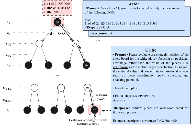
We detail our experiments conducted across three different game scenarios. For each experiment, we configure the LLM as an action pruner, allowing it to suggest what it deems as the optimal action 20 times for each state, with a temperature setting of 0.7. We set and for any for the UCB bonus defined in (4.1). We begin by exploring two initial toy experiments: chess puzzles and MiniGo, where the LLM’s role is solely to act as an action pruner. Given the shorter game horizons in these scenarios, we directly use the game’s outcome as a proxy for the value function. Specifically, outcomes of winning, losing, and drawing are assigned rewards of 1, -1, and 0, respectively. Afterwards, we will present our main experiment conducted on full chess games, where we set a finite search depth and use a hybrid of rule-based and LLM-based value function proxy as illustrated in Figure 1.
6.1 Chess Puzzle
Our first experiment setting is chess checkmate puzzles. We collect chess puzzles from lichess555https://database.lichess.org/#puzzles. The puzzles have different themes describing the topic of the puzzle, such as winning the game with style, or carrying out special moves. We pick the puzzles with themes mateInN. The corresponding descriptions are shown in Table 1.
| Theme | Description |
| mateIn1 | Deliver checkmate in one move. |
| mateIn2 | Deliver checkmate in two moves. |
| mateIn3 | Deliver checkmate in three moves. |
| mateIn4 | Deliver checkmate in four moves. |
| mateIn5 | Figure out a long () mating sequence. |
Since both the white player and the black player are possible to be the puzzle solver, we name the role corresponding to the puzzle solver as the agent, and name the other one as the opponent. We define the “depth” of a puzzle as the number of moves needed to deliver checkmate. We denote the state corresponding to the starting point of the puzzle as . For a puzzle with depth , we would know if the agent has solved the puzzle or not at step . Without loss of generality, we assume the agent is the max player and the opponent is the min player. And the agent gets a reward of 1 if he delivers checkmate within required steps, and -1 otherwise.
Since puzzles with depth 1 and 2 are quite simple, we only consider puzzles with depth . We construct the evaluation dataset corresponding to each depth by taking one hundred puzzles with the highest rating judged by lichess users. We implement our Algorithm 1 with gpt-3.5-turbo-instruct for its lower cost. We compare our method with the following baseline methods:
Vanilla LLM: The vanilla LLM method uses majority voting to pick action out of it’s proposed candidates. We set the temperature to 0.7 and set the number of chat completion choices to 20. And we use majority voting to pick the most popular legal answer from the 20 answers by the LLM. We choose gpt-3.5-turbo-instruct to conduct our experiment to align with our proposed method.
MCTS (50) and MCTS (10,000): The vanilla MCTS method with 50 and 10,000 simulations. In this chess puzzle setting, the only difference between this baseline and our proposed algorithm is the number of simulations and the action space. The action space here is the full action space instead of the pruned action space by LLM.
The results are as shown in Table 2. By combining LLM and MCTS self-play, our method outperforms both LLM and MCTS baselines by a huge margin. Even with only simulations, our method outperforms the MCTS baseline with simulations.
| Puzzle Depth | Vanilla LLM | MCTS () | MCTS () | LLM + MCTS () |
| 3 | 10% | 1% | 33% | 74% |
| 4 | 15% | 1% | 10% | 67% |
| 5 | 5% | 0% | 2% | 19% |
| 6 | 4% | 0% | 0% | 24% |
| 7 | 1% | 0% | 0% | 37% |
| 8 | 0% | 0% | 0% | 43% |
6.2 MiniGo
We use go board as another toy example. We adopt the ko rule which states that the stones on the board must never repeat a previous position of stones. We test our method and the baseline methods by letting them play as black with the initiative against a fixed opponent who adopts vanilla MCTS methods with 1,000 simulations and plays as white. Since the game on a go board is still very short, we set the depth of the MCTS to a large number so that we directly use the game’s outcome as a proxy for the value function. The outcomes of winning, losing, and drawing are assigned rewards of 1, -1, and 0, respectively. Note that the first player always has an advantage in Go. We use the territory score as our metric, which is defined by the territory of the black player minus that of the white player. We repeat the battle for 20 times and report the average score. The results are shown in Table 3. Our algorithm achieves the highest advantage against the fixed opponent.
| LLM | LLM + MCTS () | MCTS () | MCTS () |
| -8.0 | 11.9 | 1.3 | 9.5 |
6.3 Chess: Full Game
Our previous experiments on chess puzzles have shown the efficiency of LLM as MCTS pruner. In this part, we evaluate our method against the stockfish engine 666https://stockfishchess.org/ in full games. In a full game scheme, the game tree would become deep. Thus, we set a fixed MCTS search depth of and use a hybrid value function proxy composed of both a rule based centipawn evaluator and a LLM-based critic.
Rule-based critic: The rule-based critic we use calculates the piece values of the current board in centipawns. The centipawn is the unit of measure used in chess as measure of the advantage. The value of a pawn is 100 by default. We assign a value for each of piece in Table 4. Our critic evaluates the current board by subtracting the total value of the current player’s pieces by the total value of the opponent’s pieces and divide the result by 1,000. For example, if the black player has one more queen than the white player in the current board, the value evaluated by the critic for the black player is 0.9. We denote this rule-based critic as . Specifically, if the game is finished, we set this critic value as 10 for the winner or 0 if the game is a draw.
| Piece | Pawn | Knight | Bishop | Rook | Queen |
| Value | 100 | 325 | 325 | 500 | 900 |
LLM-based critic: The LLM-based critic evaluates the strategic position of the chess board such as piece coordination, pawn structure and attacking potential, focusing on positional advantage rather than the value of the pieces. It also uses centipawn as the unit of metric and we divide the result by 1,000 just like the rule-based critic. The prompt we use for LLM-based critic are shown in Figure 1. We denote the LLM-based critic as .
We combine the rule-based critic and the LLM-based critic by adding them together, i.e. . In practice, we use gpt-4 with a temperature of 0 as the backend of the LLM-based critic, and for consistency, we also use gpt-4 as the backend of the actor. To evaluate the performance, we define a score function that maps “win”, “tie”, and “lose” to , , and , respectively. We evaluate our method, the standalone LLMs and conventional MCTS by playing against Stockfish engine with different engine levels. The results are shown in Table 5. For the MCTS baseline, we run it in two way, one with a search depth of so that no critic is needed because the game is simulated to the end, and the other one with a search depth of and is equipped with only the rule-based critic same with our proposed method. However, we find that both MCTS baseline approaches failed to achieve a win or draw against the stockfish engine.
| Level | LLM + MCTS () | LLM | MCTS () |
| 1 | 0.78 | 0.35 | 0 |
| 2 | 0.73 | 0.15 | 0 |
| 3 | 0.47 | 0.05 | 0 |
7 Conclusion
In this study, we harness the unique capabilities of Large Language Models (LLMs) as black-box oracles and Monte-Carlo Tree Search (MCTS) as planning oracles to develop a novel self-play algorithm tailored for deterministic turn-based zero-sum games. Our approach positions the LLM to fulfill dual roles: firstly, as an action pruner, narrowing the breadth of the MCTS search tree, and secondly, as a value function proxy, thereby shortening the depth required for the MCTS search tree. This dual functionality enhances the efficiency and effectiveness of both methodologies.
Our research is supported by both theoretical and empirical analyses. Theoretically, we demonstrate that the suboptimality of the estimated value in our method is proportional to up to errors incurred by using LLM as critic and action pruner, where is the number of simulations and is the pruned action space. Empirically, through tests in chess and Go, we showcase our method’s ability to tackle complex problems beyond the reach of traditional MCTS, as well as to outperform the direct application of LLMs, highlighting its potential to advance the field of game theory and artificial intelligence.
References
- Achiam et al. (2023) Achiam, J., Adler, S., Agarwal, S., Ahmad, L., Akkaya, I., Aleman, F. L., Almeida, D., Altenschmidt, J., Altman, S., Anadkat, S. et al. (2023). Gpt-4 technical report. arXiv preprint arXiv:2303.08774.
- Agrawal (1995) Agrawal, R. (1995). Sample mean based index policies by o (log n) regret for the multi-armed bandit problem. Advances in applied probability, 27 1054–1078.
- Akata et al. (2023) Akata, E., Schulz, L., Coda-Forno, J., Oh, S. J., Bethge, M. and Schulz, E. (2023). Playing repeated games with large language models. arXiv preprint arXiv:2305.16867.
- Audibert et al. (2009) Audibert, J.-Y., Munos, R. and Szepesvári, C. (2009). Exploration–exploitation tradeoff using variance estimates in multi-armed bandits. Theoretical Computer Science, 410 1876–1902.
- Auer et al. (2002) Auer, P., Cesa-Bianchi, N. and Fischer, P. (2002). Finite-time analysis of the multiarmed bandit problem. Machine learning, 47 235–256.
- Azuma (1967) Azuma, K. (1967). Weighted sums of certain dependent random variables. Tohoku Mathematical Journal, Second Series, 19 357–367.
- Baier and Winands (2012) Baier, H. and Winands, M. H. (2012). Beam monte-carlo tree search. In 2012 IEEE Conference on Computational Intelligence and Games (CIG). IEEE.
- Berglund et al. (2023) Berglund, L., Tong, M., Kaufmann, M., Balesni, M., Stickland, A. C., Korbak, T. and Evans, O. (2023). The reversal curse: Llms trained on” a is b” fail to learn” b is a”. arXiv preprint arXiv:2309.12288.
- Bertsekas (2012) Bertsekas, D. (2012). Dynamic programming and optimal control: Volume I, vol. 4. Athena scientific.
- Champandard (2014) Champandard, A. J. (2014). Monte-carlo tree search in total war: Rome ii’s campaign ai. AIGameDev. com: http://aigamedev. com/open/coverage/mcts-rome-ii, 4.
- Churchill and Buro (2013) Churchill, D. and Buro, M. (2013). Portfolio greedy search and simulation for large-scale combat in starcraft. In 2013 IEEE Conference on Computational Inteligence in Games (CIG). IEEE.
- Coulom (2006) Coulom, R. (2006). Efficient selectivity and backup operators in monte-carlo tree search. In International conference on computers and games. Springer.
- Feng et al. (2023a) Feng, X., Luo, Y., Wang, Z., Tang, H., Yang, M., Shao, K., Mguni, D., Du, Y. and Wang, J. (2023a). Chessgpt: Bridging policy learning and language modeling. arXiv preprint arXiv:2306.09200.
- Feng et al. (2023b) Feng, X., Wan, Z., Wen, M., Wen, Y., Zhang, W. and Wang, J. (2023b). Alphazero-like tree-search can guide large language model decoding and training. arXiv preprint arXiv:2309.17179.
- Hao et al. (2023) Hao, S., Gu, Y., Ma, H., Hong, J. J., Wang, Z., Wang, D. Z. and Hu, Z. (2023). Reasoning with language model is planning with world model. arXiv preprint arXiv:2305.14992.
- Huang and Chang (2022) Huang, J. and Chang, K. C.-C. (2022). Towards reasoning in large language models: A survey. arXiv preprint arXiv:2212.10403.
- Huang et al. (2023) Huang, L., Yu, W., Ma, W., Zhong, W., Feng, Z., Wang, H., Chen, Q., Peng, W., Feng, X., Qin, B. et al. (2023). A survey on hallucination in large language models: Principles, taxonomy, challenges, and open questions. arXiv preprint arXiv:2311.05232.
- Justesen et al. (2014) Justesen, N., Tillman, B., Togelius, J. and Risi, S. (2014). Script-and cluster-based uct for starcraft. In 2014 IEEE conference on computational intelligence and games. IEEE.
- Kishimoto and Schaeffer (2002) Kishimoto, A. and Schaeffer, J. (2002). Transposition table driven work scheduling in distributed game-tree search. In Advances in Artificial Intelligence: 15th Conference of the Canadian Society for Computational Studies of Intelligence, AI 2002 Calgary, Canada, May 27–29, 2002 Proceedings 15. Springer.
- Kocsis and Szepesvári (2006) Kocsis, L. and Szepesvári, C. (2006). Bandit based monte-carlo planning. In European conference on machine learning. Springer.
- Liu et al. (2023) Liu, Z., Hu, H., Zhang, S., Guo, H., Ke, S., Liu, B. and Wang, Z. (2023). Reason for future, act for now: A principled framework for autonomous llm agents with provable sample efficiency. arXiv preprint arXiv:2309.17382.
- Lowerre and Reddy (1976) Lowerre, B. and Reddy, R. (1976). The harpy speech recognition system: performance with large vocabularies. The Journal of the Acoustical Society of America, 60 S10–S11.
- Mao et al. (2023) Mao, S., Cai, Y., Xia, Y., Wu, W., Wang, X., Wang, F., Ge, T. and Wei, F. (2023). Alympics: Language agents meet game theory. arXiv preprint arXiv:2311.03220.
- Pearl (1980) Pearl, J. (1980). Scout: A simple game-searching algorithm with proven optimal properties. In AAAI.
- Pepels and Winands (2012) Pepels, T. and Winands, M. H. (2012). Enhancements for monte-carlo tree search in ms pac-man. In 2012 IEEE Conference on Computational Intelligence and Games (CIG). IEEE.
- Ruoss et al. (2024) Ruoss, A., Delétang, G., Medapati, S., Grau-Moya, J., Wenliang, L. K., Catt, E., Reid, J. and Genewein, T. (2024). Grandmaster-level chess without search. arXiv preprint arXiv:2402.04494.
- Schaeffer (1989) Schaeffer, J. (1989). The history heuristic and alpha-beta search enhancements in practice. IEEE transactions on pattern analysis and machine intelligence, 11 1203–1212.
- Sephton et al. (2014) Sephton, N., Cowling, P. I., Powley, E. and Slaven, N. H. (2014). Heuristic move pruning in monte carlo tree search for the strategic card game lords of war. In 2014 IEEE conference on computational intelligence and games. IEEE.
- Shah et al. (2020) Shah, D., Xie, Q. and Xu, Z. (2020). Non-asymptotic analysis of monte carlo tree search. In Abstracts of the 2020 SIGMETRICS/Performance Joint International Conference on Measurement and Modeling of Computer Systems.
- Shridhar et al. (2020) Shridhar, M., Yuan, X., Côté, M.-A., Bisk, Y., Trischler, A. and Hausknecht, M. (2020). Alfworld: Aligning text and embodied environments for interactive learning. arXiv preprint arXiv:2010.03768.
- Silver et al. (2017) Silver, D., Schrittwieser, J., Simonyan, K., Antonoglou, I., Huang, A., Guez, A., Hubert, T., Baker, L., Lai, M., Bolton, A. et al. (2017). Mastering the game of go without human knowledge. nature, 550 354–359.
- Soemers et al. (2016) Soemers, D. J., Sironi, C. F., Schuster, T. and Winands, M. H. (2016). Enhancements for real-time monte-carlo tree search in general video game playing. In 2016 IEEE Conference on Computational Intelligence and Games (CIG). IEEE.
- Yao et al. (2023) Yao, S., Yu, D., Zhao, J., Shafran, I., Griffiths, T. L., Cao, Y. and Narasimhan, K. (2023). Tree of thoughts: Deliberate problem solving with large language models. arXiv preprint arXiv:2305.10601.
- Zhang et al. (2023) Zhang, Y., Li, Y., Cui, L., Cai, D., Liu, L., Fu, T., Huang, X., Zhao, E., Zhang, Y., Chen, Y. et al. (2023). Siren’s song in the ai ocean: A survey on hallucination in large language models. arXiv preprint arXiv:2309.01219.
- Zhou et al. (2018) Zhou, H., Gong, Y., Mugrai, L., Khalifa, A., Nealen, A. and Togelius, J. (2018). A hybrid search agent in pommerman. In Proceedings of the 13th international conference on the foundations of digital games.
Appendix A Value Estimation Error Analysis
Without loss of generality, we assume the root node correspond to the state where the max player is about to make a move. Thus, the leaf nodes correspond to the state where the min player is about to make a move. For any , denote by the number of nodes at level and denote by the nodes in at level . We denote the cardinality of the pruned action space and represent the pruned action space by . We rewrite the bonus function as
For any , we denote by
the estimated expected return for the min player at level for taking action at state , where is the input value function of Algorithm 1 as an estimation of the true value function . Since the level corresponds to the min player, we define
Then, we define recursively
| (A.1) | ||||
| (A.2) |
for any . Meanwhile, we denote by
the optimal action at state according to the value function , and by
| (A.3) |
the gap between the optimal arm and the second optimal arm at state . Furthermore, we define the empirical value functions of our Algorithm 1. For each level , denote by the sum of discounted rewards collected at state during visits of it.
A.1 Non-stationary Multi-Arm Bandit
Consider non-stationary multi-arm bandit (MAB) problems. Let there be arms or actions and let denote the random reward obtained by playing the arm for the -th time with . We assume that the optimal arm is unique. We denote by the empirical mean of the reward obtained by playing arm for times and denote by the expectation of the empirical mean. We assume that the optimal arm is unique. We make the following assumptions about the reward .
Assumption A.1.
There exists an absolute constant such that for any arm .
Assumption A.2.
The reward sequence is a non-stationary process such that
-
1.
there exists for any such that
-
2.
there exists and such that for any and ,
Assumption A.1 states that the reward is bounded for all arms. And Assumption A.2 establishes the convergence and concentration properties of the process. Those assumptions holds naturally for bounded and deterministic reward setting.
Consider the following variant of UCB algorithm applied to the above non-stationary MAB.
In Algorithm 2, is the number of times arm has been played, up to (including) time , is the upper confidence bound for arm when it is played times in total of time steps, and is the bonus term, where , are constants defined in Assumption A.2 and is a tuning parameter that controls the exploration and exploitation trade-off. A tie is broken arbitrarily when selecting an arm in Line 4.
Denote by the optimal value with respect to the converged expectation, and by the corresponding optimal arm. We assume the optimal arm is unique. Denote by the gap between the optimal arm and the second optimal arm, and define
| (A.4) |
Also, we denote by
| (A.5) |
Denote by the empirical mean reward under the Algorithm 2. The following theorem establishes theoretical analysis for Algorithm 2.
Theorem A.3 (Theorem 3, Shah et al. (2020)).
Here, is the gap between the optimal arm and the second optimal arm, and are given by (A.4) and (A.5), respectively. Theorem A.3 provides both the convergence guarantee (A.6) and the concentration guarantee (A.7) of the UCB algorithm described in Algorithm 2.
Min player counterpart.
We can construct a min player version of the non-stationary multi-arm bandit by adopting a negative bonus and choosing the arm with lowest UCB value. We include the algorithm here for completeness.
Similarly, we define , , and . Then, we mirror Theorem A.3 to give the following analysis for the min player.
A.2 Leaf Level
The leaf nodes at level are children of nodes at level in the MCTS tree. Without loss of generality, we assume the leaf nodes correspond to the state where the max player is about to make a move, the same as the root node . Therefore, the nodes at level correspond to the min player. Consider node at level , corresponding to state . Each time the min player is at this node, it takes an action and reaches the node at the leaf level . Then, the reward collected for the node and action is , where is calculated by the input value function proxy for Algorithm 1. Thus, each time the node is visited, the reward is the summation of bounded independent and identical (for a given action) random variables and a deterministic evaluation. By Lemma C.2, there exists such that the collected rewards at satisfy the concentration property (C.1) and the convergence property (C.2). This process mirrors the MAB problem we introduced in Section A.1. In order to apply Theorem A.3 or Corollary A.4, we denote by the maximum magnitude of the rewards collected by all the nodes in level and we quantify it later in Lemma C.3. Then, we have the following lemma that establishes the convergence and concentration property of the nodes in level .
Lemma A.5 (Leaf).
Consider a node corresponding to state at level within the MCTS for . Let be the total discounted reward collected at during visits of it, to one of its leaf nodes under the UCB policy. Then, there exists appropriately large such that the following holds for a given and .
-
1.
It holds that
-
2.
There exist such that it holds for any and that
Proof.
The proof follows directly from Corollary A.4. ∎
A.3 Recursion
Lemma A.5 suggests that the convergence assumption (A.6) and concentration assumption (A.7) of Theorem A.3 are satisfied by for each node at level with and defined in Theorem 5.2 and with appropriately defined large enough constant . We claim that result similar to Lemma A.5, but for node at level , continues to hold with parameters and as defined in Theorem 5.2 and with appropriately defined large enough constant . And similar argument will continue to apply going from level to for all . That is, we shall assume that the convergence and concentration assumptions of Theorem A.3 or Corollary A.4 hold for , for all nodes at level with parameters and defined in Theorem 5.2 and with appropriately defined large enough constant , and then argue that such holds for nodes at level as well. Thus, we can prove the results for all by induction.
To that end, we first consider the nodes corresponding to the max player. For any , consider a node corresponding to state at level within the MCTS for . As part of the algorithm, whenever this node is visited, one of the feasible action is taken and the node at level will be reached. This results in a reward at node at level . Since is an independent, bounded valued random variable while is effectively collected by following a path all the way to the leaf level. Inductively, we assume that satisfies the convergence and concentration property for each node at level , with and given by Theorem 5.2 and with appropriately defined large enough constant . Therefore, by an application of Lemma C.2, it follows that this combined reward continues to satisfy the convergence (A.6) and concentration (A.7) properties. Thus, we invoke Theorem A.3 and conclude the follow lemma.
Lemma A.6 (Max player).
Consider a node corresponding to state at level in the MCTS tree for . Let be the sum discounted reward collected at during visits. Then, the following holds for the choice of appropriately large , for a given and .
-
1.
It holds that
-
2.
There exist a large enough constant such that it holds for any and that
Next, we consider a node corresponding to state where the min player is about to make a move for any . Similarly, whenever this node is visited, one of the feasible action is taken and the node at level will be reached. This results in a reward at node at level . Here, the only difference is the factor, which does not effect our conclusion. By invoking Theorem A.3, we conclude the follow lemma.
Lemma A.7 (Min player).
Consider a node corresponding to state at level in the MCTS tree for . Let be the sum discounted reward collected at during visits. Then, the following holds for the choice of appropriately large , for a given and .
-
1.
It holds that
-
2.
There exist a large enough constant such that it holds for any and that
A.4 Error Analysis for Value Function Iteration
We now move to the second part of the proof. The value function iteration improves the estimation of optimal value function by iterating Bellman equation. In effect, the MCTS tree is “unrolling” steps of such an iteration. Specifically, let denote the value function before an iteration, and let be the value function after iteration. By definition, it holds for any ,
| (A.10) |
Recall that value iteration is contractive with respect to norm (Bertsekas, 2012). That is, for any ,
| (A.11) |
Since we can flipping the sign of , and without breaking the contractive nature, the following iteration is also contractive with respect to norm,
| (A.12) |
Thus, (A.11) still applies to the iteration corresponding to (A.12). By drawing connection between (A.1) and (A.10) as well as (A.2) and (A.12), we conclude the following lemma.
Lemma A.8.
The mean reward collected under the MCTS policy at root note , starting with input value function proxy is such that
| (A.13) |
A.5 Completing Proof of Theorem 5.2
In summary, using Lemma A.5 and A.6, we conclude that the recursive relationship going from level to and from level to holds for all with level being the root. We set and . At root , the query state that is input to the MCTS policy, we have that after total simulations of MCTS, the empirical average of the rewards over these trial, is such that using the fact that
| (A.14) |
where the last equality follows from . By Lemma A.8, it holds that
| (A.15) |
since . Combining (A.14) and (A.15), it then holds that
| (A.16) |
This concludes the proof of Theorem 5.2.
Appendix B Pruning Analysis
B.1 Proof of the property of LSE
Proof of Lemma 5.3.
Denote by . For any , we have
| (B.1) |
where the first equality uses the definition of and the first inequality uses the fact that for any and .
Note that
| (B.2) | |||
| (B.3) |
where we use the definition of and the fact that .
B.2 Proof of the pruning error bound
Proof of Proposition 5.5.
By the notion of half-horizon, we mirror (3.5) to define
| (B.5) |
Combining (5.3), (B.5), and the fact that , we have
| (B.6) |
For the notational simplicity, we define as
| (B.7) |
where we define as , as , and as
| (B.8) |
for any .
By the definition of in (B.7), we use triangle inequality to have
| (B.9) |
Invoking Lemma 5.3, we have
| (B.10) |
for any . Plugging (B.9) and (B.10) into (B.7), we bound as follows,
| (B.11) |
for any . Here, the inequality uses the definition of in Definition 5.4. By (3.6), we have
| (B.12) |
for any and . Here, the first inequality uses the definition of in Definition 5.4 and the triangle inequality, the second inequality uses the contraction property of operator, and the last inequality uses the fact that . Take the maximum for on the left-hand side of (B.12), we obtain
| (B.13) |
for any . Emulating the similar proof, we have
| (B.14) |
for any and . Here, the first inequality uses the definition of in Definition 5.4 and the triangle inequality, the second inequality uses the contraction property of operator, and the last inequality uses the fact that . Take the maximum for on the left-hand side of (B.14), we obtain
| (B.15) |
for any . Combining (B.13) and (B.15), we have that
for any . Here, the last inequality uses (B.11). Thus, we finish the proof of Proposition 5.5. ∎
Appendix C Auxiliary Lemmas
Lemma C.1 (The Azuma-Hoeffding’s Inequality (Azuma, 1967)).
Let be independent random variables such that almost surely. It then holds for any that
Lemma C.2.
Consider random variables for such that ’s are independent and identically distributed taking values in for some and ’s are independent of ’s. Suppose there exists such that it holds for any that
and it holds for any and that
where , , are constants. Let for some , and let be the expectation of all ’s. Then, it holds for any that
| (C.1) |
And it holds for any and that
| (C.2) |
where .
Proof.
Following from Lemma C.1 and the fact that ’s are i.i.d. bounded random variables taking value in , it holds for any that
Thus, it holds for a large enough constant that
To choose a proper value value , note that
where the first inequality follows from the fact that and , and the second inequality is obtained via treating the right-hand side as a function of and finding the maximum of that function. Then, we conclude the proof of the first equation in (C.2) by setting
We can prove the second equation by the same reasoning. ∎
Lemma C.3 (Maximum magnitude).
Denote by the maximum magnitude of the rewards collected by all the nodes in level . It then holds for any that
| (C.3) | ||||
| (C.4) | ||||
| (C.5) |
Proof.
Since all the rewards are bounded by . Then it follows from the definition of and in (3.5) and (3.6) that
The rewards collected for the node and action at level is . Since the is provided by the input value function proxy of Algorithm 2 and , it holds that
For any , the rewards collected for the node and action at level is
and for level ,
which concludes the proof of Lemma C.3. ∎