Hawai‘i Supernova Flows: A Peculiar Velocity Survey Using Over a Thousand Supernovae in the Near-Infrared

Abstract

We introduce the Hawai‘i Supernova Flows project and present summary statistics of the first 1218 astronomical transients observed, 669 of which are spectroscopically classified Type Ia Supernovae (SNe Ia). Our project is designed to obtain systematics-limited distances to SNe Ia while consuming minimal dedicated observational resources. This growing sample will provide increasing resolution into peculiar velocities as a function of position on the sky and redshift, allowing us to more accurately map the structure of dark matter . This can be used to derive cosmological parameters such as $\sigma_{8}$ and can be compared with large scale flow maps from other methods such as luminosity–line width or luminosity–velocity dispersion correlations in galaxies. Additionally, our photometry will provide a valuable test bed for analyses of SNe Ia incorporating near-infrared data. In this survey paper, we describe the methodology used to select targets, collect and reduce data, and calculate distances.

1 Introduction

Hawai‘i Supernova Flows is an ongoing effort to map the distribution of mass in the local universe (z < 0.1) using near-infrared (NIR) observations of Type Ia Supernovae (SNe Ia) in combination with untargeted optical surveys. In this paper we provide an overview of the Hawai‘i Supernova Flows project to support future papers examining detailed science cases using data from Hawai‘i Supernova Flows.

1.1 Peculiar Velocities and the State-of-the-Art

While the Large Scale Structure (LSS) contains some luminous, baryonic matter, the majority of its mass may only be studied through its gravitational effects (for a review of dark matter, consider Bertone & Hooper, 2018). In comoving coordinates, objects accelerate towards denser regions of LSS and away from voids. This motion is called peculiar velocity and its projection on our line of sight may be calculated as (Davis & Scrimgeour, 2014)

$$v=c\leavevmode\nobreak\ \left(\leavevmode\nobreak\ \frac{z_{\mathrm{obs}}-z_{\mathrm{cos}}(d_{L})}{1+z_{\mathrm{cos}}(d_{L})}\leavevmode\nobreak\ \right)$$ (1)

where $z_{obs}$ is the observed redshift and $z_{cos}(d_{L})$ is the redshift at luminosity distance $d_{L}$ due to universal expansion in a given cosmological model with deceleration parameter $q_{0}$ and Hubble constant $H_{0}$ (Peebles, 1993)

$$z_{\mathrm{cos}}\approx\frac{1}{1-q_{0}}\left[-1+\sqrt{1+\frac{2H_{0}d_{L}}{c}(1-q_{0})}\right].$$ (2)

Peculiar velocities have been used to infer the distribution of LSS through a variety of approaches like the POTENT method (Bertschinger & Dekel, 1989; Dekel et al., 1990, 1999), the Wiener Filter and constrained realizations method (Ganon & Hoffman, 1993; Zaroubi et al., 1995; Zaroubi et al., 1999; Courtois et al., 2012), the unbiased minimal variance estimator (Zaroubi, 2002), and various Bayesian hierarchical approaches (Lavaux, 2016; Graziani et al., 2019; Valade et al., 2022). These methods commonly assume the LSS formed through gravitational instabilities, and is thus irrotational on large scales ($\nabla\times\vec{v}=0$) (Peebles, 1980). Variations between the methods typically represent different approaches to minimizing the systematic effects of smoothing, uneven sky coverage, and biases in peculiar-velocity surveys. Modern cosmographic surveys are not limited by analytical tools, but by the number and precision of distance measurements.

Many peculiar velocity surveys use either the Fundamental Plane (FP; Djorgovski & Davis, 1987; Dressler et al., 1987) or the Tully-Fisher relation (TF; Tully & Fisher, 1977) to measure distances because these methods can be applied to a significant fraction of all galaxies, whereas other methods require relatively rare phenomena like a gravitational lens (Refsdal, 1964), a maser (Herrnstein et al., 1999) or megamaser (Gao et al., 2016), a gravitational wave event (Holz & Hughes, 2005), or a supernova (SN). However, while the FP and TF methods have significant advantages in target availability, the resulting distance measurements are often five to ten times less precise than measurements from more narrowly applicable distance probes. The FP and TF methods, along with most photometric measures of distance, produce errors in distance modulus, which causes error to increase with the distance. This proportionality is directly passed on to the uncertainties in peculiar velocity. While independent peculiar velocity measurements of $N$ neighboring galaxies can be combined to reduce the statistical uncertainty by a factor of $\sqrt{N}$, galaxies have a finite amount of neighbors. A volume-limited peculiar velocity survey will always find a noise floor that scales with the uncertainty in the distance-measuring technique and inversely with the root of galaxy number density. Put another way, a survey with an explicit precision requirement has a maximum effective range that cannot be extended without more precise measures of distance.

For this reason, two of the three largest homogeneous collections of peculiar velocities extend no farther than a cosmic microwave background (CMB) rest-frame redshift of $z_{\text{CMB}}=0.05$. These are the Cosmicflows-IV TF catalogue (CF4-TF, 9792 galaxies; Kourkchi et al., 2020) and the FP-based 6-degree Field Galaxy Survey peculiar velocity sample (6dFGSv, 8885 galaxies; Springob et al., 2014; Campbell et al., 2014). The Sloan Digital Sky Survey (SDSS) peculiar velocity catalogue (SDSS-PV, 34059 galaxies; Howlett et al., 2022) is the first FP- or TF-based survey to extend to $z_{\text{CMB}}=0.1$, but so far only covers the SDSS North Galactic Cap contiguous area (7016 deg²). The largest compilation of extragalactic distances is the heterogeneous catalogue Cosmicflows-IV (CF4, 55877 galaxies; Tully et al., 2023), which consolidates these and other surveys and uses both FP and TF measurements, as well as surface brightness fluctuations (Tonry & Schneider, 1988), core-collapse SNe (Hamuy & Pinto, 2002), and SNe Ia (Phillips, 1993).

The SDSS-PV sample has not yet produced any detailed cosmographic studies, but the authors measured a bulk flow in mild excess of what a fiducial $\Lambda$CDM model would suggest. This excess has been suggested before using various independent data sets (e.g. Pike & Hudson, 2005; Feldman & Watkins, 2008; Kashlinsky et al., 2008; Lavaux et al., 2010; Feldman et al., 2010). Contemporary analyses extend the scale of the issue, with Watkins et al. (2023) finding that CF4 data indicate excess bulk flows on scales of 200 h^-1 Mpc that have a $1.5\times 10^{-6}$ chance of occurring in the standard cosmological model using CMB-derived parameters. Howlett et al. (2022) theorize that the Shapley Supercluster as seen in the 2M++ redshift compilation (Carrick et al., 2015) could be responsible, but because it is not in the SDSS-PV survey footprint it will be difficult to test. A survey that trades depth for sky coverage will still struggle to constrain the effects of the Shapley Supercluster, as Carrick et al. (2015) find their bulk flow measurements prefer a contribution from sources at $z>0.067$ at a 5.1$\sigma$ level.

Thus far, the Hawai‘i Supernova Flows project has obtained peculiar velocity measurements over three quarters of the sky to a depth of $z\sim 0.1$. This encompasses the gravitational sources thought to dominate local dynamics, including the Shapley supercluster, the Dipole repeller (Hoffman et al., 2017), and the Cold Spot repeller (Courtois et al., 2017). Equation 1 shows that peculiar velocities require an assumed cosmology and two measurements: an observed redshift and a proper distance. The redshift can be measured to relatively high precision with a single spectrum, but measuring distances is more difficult. Techniques have been developed and refined to excel in various niches of a parameter space spanning applicability, maximum range, and precision. Our project uses optical and NIR observations of SNe Ia to measure distances.

1.2 Type Ia Supernovae

Following the discovery that SNe Ia could be used as standardizable candles (Pskovskii, 1977; Phillips, 1993; Tripp, 1998) there have been continuous efforts to improve the accuracy and precision of SNe Ia distance inference. These efforts include refining theoretical models of SNe Ia progenitors and explosions (reviewed in Liu et al., 2023); increasing the sample of well-studied SNe Ia (e.g. Amanullah et al., 2010; Scolnic et al., 2018; Phillips et al., 2018; Brout et al., 2022); and empirically identifying correlations between SNe Ia luminosities and observable parameters like host-galaxy mass (Kelly et al., 2010; Lampeitl et al., 2010; Sullivan et al., 2010), host-galaxy specific star formation rate (Uddin et al., 2017), local H_α surface brightness (Rigault et al., 2013), host-galaxy metallicity (Moreno-Raya et al., 2016), host-galaxy colours (Roman et al., 2018), ejecta velocity (Léget et al., 2020), and more. Accompanying these efforts are improvements to fitting and modelling techniques (BayeSN, Mandel et al. (2009); Mandel et al. (2011); Thorp et al. (2021); Mandel et al. (2022); Grayling et al. (2024); MLCS2k2, Jha et al. (2007); SALT, Guy et al. (2005, 2007, 2010); Kenworthy et al. (2021); Pierel et al. (2022); SiFTO, Conley et al. (2008); SNEMO, Saunders et al. (2018); SNooPy, Burns et al. (2011, 2014); SUGAR, Léget et al. (2020)). This body of work has established SNe Ia as excellent probes of distance. We choose to use them over competing distance measuring techniques for three reasons.

Firstly, SNe Ia are abundant. With modern surveys across the globe constantly scanning the sky, SNe are no longer rare targets of opportunity, but are discovered every night. Desai et al. (2024) use data from the All-Sky Automated Survey for SuperNovae (ASAS-SN; Shappee et al., 2014; Kochanek et al., 2017; Hart et al., 2023) to find a SN Ia volumetric rate of $\sim 2.3\times 10^{4}\text{ yr}^{-1}\text{ Gpc}^{-3}h^{3}_{70}$, which amounts to about 20 each night within $z<0.1$. Wiseman et al. (2021) use results from the Dark Energy Survey (DES) to calculate a rate of SNe Ia per galaxy between 1 every 3,000 years to more than one every 100 years depending on host-galaxy properties. This means that although the number of usable galaxies in a SNe Ia-based peculiar velocity survey is relatively low compared to TF or FP surveys, it scales with time and can exceed competing methods with enough observational support.

Secondly, SNe Ia are bright enough to be used at the distances we require. The demonstration of accelerating expansion relied on measurements of SNe Ia at redshifts near unity (Riess et al., 1998; Perlmutter et al., 1999). Our interests are much more local, extending to redshifts $z<0.1$. The mean absolute magnitude of SNe Ia before correcting for host-galaxy extinction is about $-18.6$ mag in $B$ and $-18.7$ mag in $V$ (e.g. Ashall et al., 2016). At $z=0.1$ this corresponds to an apparent magnitude of about 19.6 or 19.5 mag, within the limiting magnitude of two of the all-sky surveys described in Sec. 2.1.

Lastly, SNe Ia-based distance measurements are far more precise than those of competing methodologies. This is not to say that SNe Ia are the most precise of all distance indicators. Distances based on Cepheid period-luminosity relations (Leavitt & Pickering, 1912) or the Tip of the Red Giant Branch (Freedman et al., 2020; Anand et al., 2021) are typically more precise than those based on SNe Ia, but the objects of study for these probes are about 13-16 magnitudes fainter than SNe Ia. This restricts them to $z<0.023$ even with 22 HST orbits per galaxy (PI D. Jones; proposal 16269). Hawai‘i Supernova Flows extends about 4 times farther. The SDSS-PV sample has used the FP method to measure distances at $z\sim 0.1$, but these distances are only precise to around 20%. SNe Ia-based distances can be systematically corrected to a root mean square (RMS) scatter between 4-7% (Burns et al., 2018; Scolnic et al., 2018). This means that it would take several dozens of independent TF or FP measurements to reach the precision of a single SN Ia distance measurement.

Optical SNe Ia light-curves have been used as standardizable candles for several decades (Phillips, 1993; Hamuy et al., 1995; Riess et al., 1998; Perlmutter et al., 1999, e.g.), but a growing body of evidence (e.g. Kasen, 2006; Wood-Vasey et al., 2008; Burns et al., 2011; Dhawan et al., 2018; Avelino et al., 2019) suggests that the NIR may offer substantial advantages.

1.2.1 SNe Ia in the Near-Infrared

NIR bandpasses like $Y$, $J$, $H$, and $K$ are 5-11 times less affected by dust than the traditionally used B band (Cardelli et al., 1989; O’Donnell, 1994; Fitzpatrick, 1999). The total-to-selective extinction parameter $R_{V}$ is known to vary based on the properties of dust, even in our own galaxy (Draine, 2003). Brout & Scolnic (2021) and Popovic et al. (2023) proposed that the dispersion in Hubble residuals of red SNe Ia may be largely due to the uncertain properties of extragalactic dust, which varies as a function of position in the host galaxy. The effects of dust correlate with the colour of any given SN Ia, making any added uncertainty a systematic issue that may not be resolved with a larger sample. Studying SNe Ia in the NIR suppresses the systematic error associated with dust.

Additionally, SNe Ia have been claimed to be more uniform in the NIR (e.g. Wood-Vasey et al., 2008; Kattner et al., 2012; Barone-Nugent et al., 2012; Stanishev et al., 2018; Avelino et al., 2019; Galbany et al., 2022; Jones et al., 2022). Avelino et al. (2019) used NIR light curves to determine distances consistent with those determined using optical light curves. Notably, Avelino et al. (2019) did not apply the typical standardizations to the NIR light curves, but did correct the optical light curves for decline rate, host-galaxy extinction, and host-galaxy mass. The empirical regularity of SNe Ia peak magnitudes in the NIR is supported by theory (Kasen, 2006), with radiative transfer calculations showing how decreases in bolometric flux are balanced by increases in relative emission at longer wavelengths. The remarkable uniformity of SNe Ia peak absolute magnitudes in the NIR makes any distance measurement much more robust against systematic uncertainties.

The paper is organized as follows. Section 2 describes the individual components of the project: including the target selection process, the observing facilities used, the photometric calibration and analysis, the identification of host galaxies, and the determination of their redshifts. Section 3 describes the three SN Ia fitting procedures we employ and how each set of fitting parameters is converted to distance moduli. We validate our fitting methodology and photometry using data from the Dark Energy, $H_{0}$, and peculiar Velocities using Infrared Light from Supernovae survey (DEHVILS; Peterson et al., 2023) and the Carnegie Supernova Project’s third data release (CSP-I DR3; Krisciunas et al., 2017) in Section 4. Section 5 lists the quality cuts used to define the various samples we describe, analyse, and discuss in Section 6.

2 Project Components and Observational Facilities

Initial testing showed that SNe Ia observations spanning the NIR-peak produce RMS dispersions in Hubble residuals $\sim 10-30\%$ lower than values obtained for SNe Ia only observed after the peak. Thus, to obtain distances to SNe Ia and recessional velocities for their host galaxies, we require three types of data: high-cadence photometry to find SNe Ia before they reach their NIR peaks, NIR photometry of each SN Ia near their peaks, and spectroscopically determined redshifts of their host-galaxies.

Figure 1 illustrates the various components of the program, delineating what is supplied from the community and what requires dedicated observing resources.

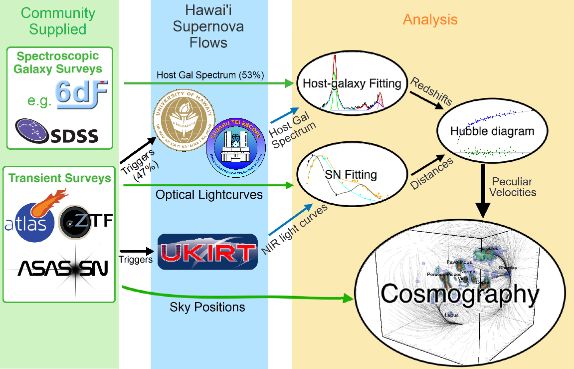
Figure 1: Our project uses archival and survey data as a foundation for supplementary observations. Whenever a new transient is reported, we collect optical light curves from ATLAS, ASAS-SN, and ZTF. We trigger NIR observations for targets that are either classified as SNe Ia or are unclassified and have a SN Ia-like light curve. About 53% of targets we observe are associated with galaxies that have spectroscopic redshifts, and we pursue spectroscopic observations for the remaining 47% with either the UH 2.2 m telescope or Subaru depending on their surface brightness profiles. The optical and NIR light curves allow us to infer luminosity distances, which we combine with host-galaxy redshifts to derive peculiar velocities.

2.1 Triggers from All-Sky Surveys

The entire sky is imaged multiple times per night thanks to All-Sky Surveys like the Asteroid Terrestrial-impact Last Alert System (ATLAS; Tonry et al., 2018), the Zwicky Transient Facility (ZTF; Bellm et al., 2019), and ASAS-SN. These surveys operate with different cadences and depths to cover a range of science cases, but they all fundamentally search the sky for objects that vary on timescales of hours, days, or months. SNe Ia are firmly in this class of astronomical objects, with light curves that increase in brightness for a few weeks before peaking, declining over a month, and then exponentially decaying. Here we describe the archival and observational facilities used, and how we access, store, and process the data.

2.1.1 The Transient Name Server

The Transient Name Server (TNS) is the official International Astronomical Union repository for extra-galactic transients. Large observational campaigns such as Pan-STARRS (Chambers et al., 2016), GaiaAlerts (Gaia Collaboration et al., 2016, 2018), the surveys described in the following sections, and many more automatically generate reports within minutes to hours of exposure read-out. Averaging overall reports from TNS, about 10% of transients receive observational follow-up and spectroscopic classification, and of these, about 70% are SNe Ia. The majority of transients fade and become unobservable without being classified.

The Hawai‘i Supernova Flows project uses the TNS-provided Python code to solicit new and recently updated reports every half hour, and uses these reports to generate a list of SNe Ia candidates. We ignore transients that are classified as anything other than a SN Ia or non-peculiar sub-type, but still consider unclassified transients as potential SNe Ia. This leads to some NIR observations of targets that are later classified as non-SN Ia, but we cannot afford to wait for spectroscopic classification of each target, which often occurs after the NIR-peak as seen in Fig. 2.

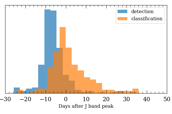
Figure 2: The distribution of detection dates and public classification dates for SNe Ia relative to the $J$-band maximum light. About 40% of all SNe Ia are classified more than a day before the NIR peak.

The reduction in efficiency can be mitigated in several ways. The Hawai‘i Supernova Flows team relays targets of interest to the Spectroscopic Classification of Astronomical Transients (SCAT) program (Tucker et al., 2022). The SCAT team classifies astronomical transients using spectra primarily from the UH 2.2 m telescope’s SNIFS instrument (described in more detail in section 2.3.3), but has recently expanded to the ANU 2.3 m through a collaboration with Melbourne University. In a random sampling of TNS objects, one would expect 10% to be classified, but by providing SCAT with a list of candidates to observe, we increase the fraction of classified transients in our observed sample to about 73%. Additionally, Möller & de Boissière (2020) demonstrated that using whole light-curves, SNe Ia and non-SNe Ia can be identified with up to 95% accuracy, or 98% accuracy when including host-galaxy information. Even when restricting the light curves to early times, the difference in light-curve shape between various SNe allows us to avoid observing unclassified targets that are unlikely to be SNe Ia. The demographics of Hawai‘i Supernova Flows targets are presented in Table 1.

Type	Number
SN Ia-norm	637
SN Ia-91T-like	26
SN Ia-91bg-like	6
Unclassified	328
SN Ia-pec	3
SN Ia-CSM	2
SN Iax[02cx-like]	2
SN Ia-SC	1
SN II	93
SN IIn	15
SN Ic	12
SN Ib	11
CV	7
SN IIP	6
SN	4
SN Ibn	4
SN Ib/c	3
SN I	3
SN Ic-BL	3
Nova	2
SLSN-II	1
LRN	1
AGN	1
SN Ib-Ca-rich	1
Varstar	1
SLSN-I	1
Impostor-SN	1
ILRT	1

Table 1: The spectroscopic classifications of our observed targets show that a strong majority of our targets receive classification, and most of those classifications are some kind of SN Ia. We need to select targets before they are classified in order to observe the NIR peak, which precedes the optical peak by several days. This results in some observations of non-SN Ia objects, but these targets are promptly removed from the observing queue.

The following sections describe three untargeted surveys with publicly available light-curve generation services that we use to improve our triggering process, and as later detailed in section 3, improve our distance determinations.

2.1.2 ATLAS

ATLAS consists of four fully robotic, 0.5 m f/2 Wright Schmidt telescopes that image the entire night sky about once every two days (Tonry, 2011; Tonry et al., 2018). This system was designed to identify potentially hazardous asteroids, and optimizations for that purpose affect the utility of ATLAS in studying astrophysical transients.

An object’s orbital elements are fairly decoupled from its spectral properties, so to increase throughput ATLAS uses two non-standard broad filters, a ‘cyan’ filter covering 420–650 nm and an ‘orange’ filter covering 560–820 nm. This aids its primary science mission by increasing “survey speed” (Tonry, 2011), but presents unique challenges for integrating observations with other filter systems which we describe in section 3.1.

Additionally, to specialize in moving object detection, the telescope system observes each field of view with four 30-second exposures over a one-hour interval. Under nominal conditions, each 30-second exposure reaches a median $5\sigma$ detection limit of $o\sim 19.1$ AB mag and $c\sim 19.6$ AB mag. For stationary targets, these exposures can be co-added to improve depth by about 0.75 AB mag and increase the Signal-to-Noise-Ratio (SNR) at a given brightness by a factor of 2. However, we found that inter-observational variation in point spread function (PSF), pointing, and atmospheric conditions made combining multiple exposures difficult. Instead, we combine the four photometric measurements of each object using an inverse variance weighted median, excluding any measurement more than three times its uncertainty away from the median flux. Additionally, we ignore measurements where the object is within 40 pixels of a chip edge or has an axis ratio greater than 1.5 and measurements where the sky brightness is under 16.

Although ATLAS specializes in astronomy at the Solar System scale, it is a leading source of high-cadence data for studying astrophysical transients. Smith et al. (2020) describe the utility of ATLAS in this context and how to access data using the ATLAS Forced Photometry server. Hawai‘i Supernova Flows continues to use the proprietary channel we developed to access light curves before the forced photometry server came online, but the data collected exactly match the publicly available data.

2.1.3 ASAS-SN

ASAS-SN is a globally distributed system of 20 fully robotic telescopes focused on discovering bright, nearby SNe (Shappee et al., 2014; Kochanek et al., 2017; Hart et al., 2023). Each of the five ASAS-SN sites employs four 14 cm telescopes sharing a common mount. The original two sites used the Johnson V-band filter, but since 2019 all observations use the Sloan g-band filter (Holoien et al., 2020). Each pointing consists of three dithered 90 second exposures, reaching median $5\sigma$ detection limits of 17.8 AB mag each (Kochanek et al., 2017). These exposures can be co-added to improve depth by about 0.6 AB mag and increase SNR by a factor of $\sqrt{3}$. The system images the entire sky about once every 20 hours, with few losses due to weather because of the numerous sites.

The ASAS-SN light-curve server described in Kochanek et al. (2017) has grown into the ASAS-SN Sky Patrol, which serves light-curves for any position on the sky. As with ATLAS, we access this publicly available data using a proprietary channel to minimize overheads.

2.1.4 ZTF

ZTF uses the Palomar 48-inch Schmidt telescope to pursue science objectives across a range of cadences, depths, and areas, with a heavy emphasis on SNe (Bellm et al., 2019; Graham et al., 2019). Through the public surveys, ZTF covered the night sky North of $\delta=-31\degree$ once every three days, accelerating to once every two days with ZTF-II.

ZTF uses custom g-, r-, and i- band filters designed to avoid prominent sky lines at the Palomar site. These filters reach 30-second exposure $5\sigma$ limiting magnitudes of 20.8, 20.6, and 19.9 mag respectively. Each field of view is typically imaged twice, once in ZTF-g and once in ZTF-r (Bellm et al., 2019).

The ZTF alert distribution system typically produces over a million alerts each night, which feed into brokers that parse the data and make it publicly available. We access ZTF light-curves through the Automatic Learning for the Rapid Classification of Events (ALeRCE) broker’s Python client (Förster et al., 2021).

2.1.5 Triggering Criteria

When our half-hourly sync with TNS reveals a new target, we obtain light-curves from ATLAS and ZTF, and if the target is brighter than 18 mag in any filter we also obtain an ASAS-SN light-curve. We then attempt to fit the data to a SN Ia model using SNooPy (Contreras et al., 2010; Burns et al., 2011) and SALT3-NIR (Pierel et al., 2022) (our fitting procedure is discussed further in Section 3). We manually inspect the light-curves and fits to address two points: is the candidate consistent with a SN Ia and is it possible to obtain observations at or before the NIR peak? If the candidate does not have spectroscopic classification, we assess the quality of successful fits. If the residuals indicate a poor fit to the data, or if the reduced $\chi^{2}$ is greater than 2, we reject the candidate or defer judgment until more photometry becomes available. We estimate the time of peak brightness in the NIR using the best-fitting SALT3-NIR parameters. If the candidate is either classified as a SN Ia or is photometrically consistent with one, and if it has not yet reached its NIR peak, we pursue NIR observations as described in the following section.

2.2 Hawai‘i Supernova Flows NIR Photometry

2.2.1 UKIRT – WFCAM

For NIR observations, Hawai‘i Supernova Flows uses the Wide Field Camera (WFCAM) mounted on the UKIRT 3.8 m telescope owned and operated by the University of Hawai‘i (Hodapp et al., 2018). UKIRT is a 3.8-m Cassegrain telescope on the summit of Maunakea. It has a declination limit of $-40\degree<\delta<60\degree 07^{\prime}$, granting access to about 3/4 of the sky. The Cambridge Astronomical Survey Unit (CASU) continues to provide data processing services and the Wide Field Astronomy Unit at the University of Edinburgh maintains the WFCAM Science Archive (Hambly et al., 2008) through which data are distributed.

WFCAM is a NIR imager developed specifically for large-scale surveys (Casali, M. et al., 2007). Its four detectors are Rockwell Hawaii-II (HgCdTe $2048\times 2048$) arrays (Hodapp et al., 2004) each covering $13.65^{\prime}\times 13.65^{\prime}$ at a scale of about 0.4 arcseconds / pixel. With its $0.9\degree$ diameter focal plane, WFCAM enabled the UKIRT Infrared Deep Sky Survey (Lawrence et al., 2007) and the UKIRT Hemisphere Survey (Dye et al., 2018). Hodgkin et al. (2009) explain that an astrometric distortion causes the pixel scale to vary radially, with percent level differences in pixel area between the centre and edge of the focal plane. This changes the flux from the sky in each pixel, but their Equation 1 provides a method for correcting this effect. We confirm this spatial variation and its resolution through the provided correction.

WFCAM uses a set of five broad-band filters, ZYJHK, and two narrow-band filters, H2 1-0 S1 and 1.644 FeII. Each detector is equipped with its own set of filters, with inter-detector filter variations leading to photometric differences of no more than 0.01 mag (Hewett et al., 2006). The performance of WFCAM in the above filters were analysed in Hodgkin et al. (2009), who compared instrumental magnitudes against the Two Micron All Sky Survey (2MASS) Point Source Catalog (Skrutskie et al., 2006). We use the $J$-band colour equation they derive to convert 2MASS $J$ and $H$ magnitudes to WFCAM $J$ magnitudes, which we use to calculate zero-points for each image.

Hodgkin et al. (2009) also identified spatially correlated photometric variability, even when accounting for the astrometric distortion mentioned previously. The exact cause of the issue is unknown, but CASU provides an empirically derived table of corrections on a monthly basis. We address this spatial correlation independently by treating each image’s zero-point as a 2nd-order two-dimensional polynomial centred on the SN candidate, inferred with the probabilistic programming language Stan for each image (Carpenter et al., 2017). The scale of the effect is $\sim$0.021 mag from the centre to the edges of the image, comparable to the tables provided by CASU.

2.2.2 Source Characterization and Galaxy Subtraction

The data distributed through the WFCAM Science Archive include catalogues of photometric parameters for sources extracted with the program imcore. Initial testing highlighted issues in the catalogues when point sources coincided with extended sources. This compromised the photometry of most SNe Ia that were not exceptionally well separated from their host-galaxy.

Leveraging the multiplicity of our observations, we analysed each supernova and host-galaxy image series as an ensemble using the forward-model (or scene-model) code from Rubin et al. (2021). In short, this procedure assumes a series of images contains a time-independent two-dimensional surface (modelled with splines) and a time-varying point-source. This allows for degeneracies when ‘sharp’ features in the galaxy (such as the nucleus) coincide with the SN Ia, but late-time observations of the galaxy taken after the SN Ia has faded resolve this issue by essentially providing a traditional reference image for subtraction. We manually determine which host-galaxies require late-time observations using diagnostic images such as those in Figure 3. We pursue late-time observations if the galaxy model exhibits sharp features at the site of the SN, or if the residuals after subtracting either the galaxy or the galaxy and SN appear to have spatial structure.

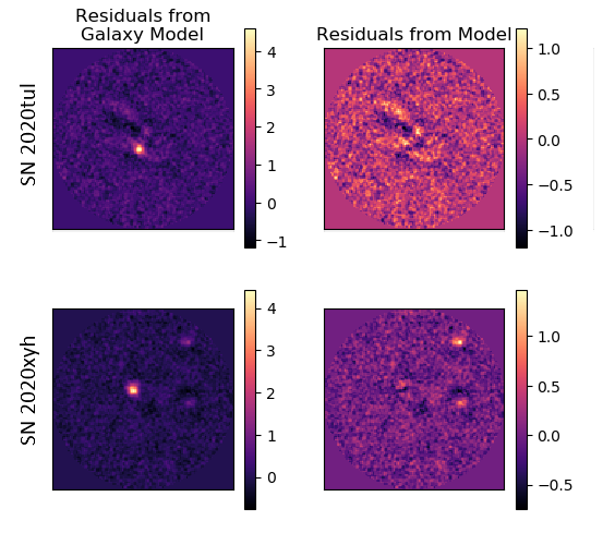
Figure 3: The forward-modelling code used to make photometric measurements produces diagnostic images showing the observed flux, the galaxy model, the residuals after subtracting the galaxy model (‘Residuals from Galaxy Model’), and the residuals after subtracting both the galaxy and supernova models (‘Residuals from Model’). We present a few examples representative of bad subtractions. SN 2020tul shows spatially correlated structure after galaxy subtraction, indicating the galaxy was not accurately modeled. Additionally, the supernova appears oversubtracted. This effect is more clearly seen in SN 2020xyh, which occurred near the nucleus of its host galaxy. The images on the left seem to show the galaxy has been subtracted, leaving only point sources at the location of the supernova and two nearby galaxies, but the images on the right show that SN 2020xyh appears to leave a small hole in some unmodelled structure.

We use the subsample of targets with late-time observations to validate our methodology against an independent data reduction process using traditional image subtraction performed with ISIS (Alard & Lupton, 1998, 1999) and source characterization using tphot (Sonnett et al., 2013). The differences between the forward-modelled and image-subtracted photometry have a median of 0.008 mag and a standard deviation of 0.07 mag. We also examine how the forward-modelling code performs without late-time observations, and find the median difference remains low at 0.02 mag, but the standard deviation increases significantly to 0.826 mag. This increase is driven by a few cases where the forward-modelling code struggled to separate the galaxy and the transient. Figure 4 shows the average difference in a galaxy’s forward-modelled photometry with and without late-time observations as a function of projected separation between the supernova and host-galaxy nucleus. The histogram shows that in the majority of cases, late-time observations do not result in significantly different photometry. In a few cases, the observations break degeneracies in the forward-modelling process, resulting in photometry up to a few magnitudes different. These cases are visually conspicuous, as seen in Figure 3. In Appendix A, we fit a Gaussian mixture-model to the photometric differences ($\Delta m$) using Stan (Carpenter et al., 2017) and find 83.3% of the differences appear tightly dispersed ($\Delta m\sim\mathcal{N}(0.02\pm 0.006\text{ mag},0.08\pm 0.007\text{ mag})$), and the remaining 16.7% vary much more dramatically ($\Delta m\sim\mathcal{N}(0.37\pm 0.131\text{ mag},0.94\pm 0.110\text{ mag})$). The fraction of targets reliant upon late-time observations for accurate photometry is vastly exaggerated in this analysis because the subsample comprises only targets manually determined to potentially benefit from late-time observations. Forward-modelled photometry is thus as accurate as traditional image subtraction, and more economical in that it often does not require a late-time observation.

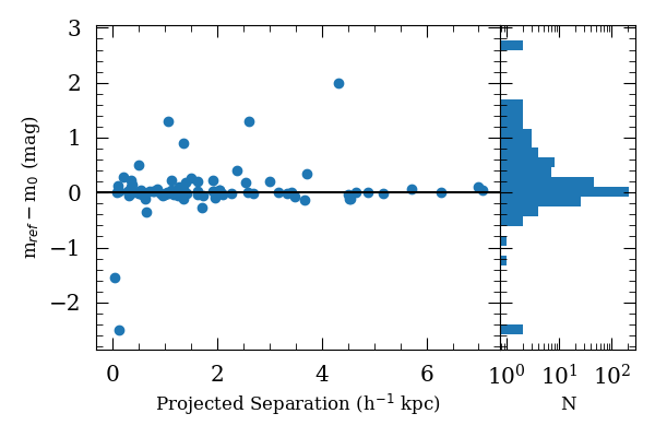
Figure 4: The differences between measurements made with and without late-time observations are minimal for a large number of targets, indicating accurate reconstruction of the galaxy surface profile. However, there are many targets where a late-time observation is crucial for decoupling the SN and host galaxy. The abundance of targets needing late-time observation is biased high in the plotted data because all targets were manually determined to potentially benefit from late-time observations.

2.3 Host Galaxy Redshifts

Although dozens of surveys have collectively measured redshifts for millions of galaxies, about half of the SNe Ia in our sample have host galaxies with no publicly available redshifts. Furthermore, the redshift measurements that are publicly available come from heterogeneous methodologies and at times are inconsistent with other measurements of the same galaxy. Here we describe how we identify host-galaxies for each SN Ia, incorporate data from extant surveys, and obtain redshifts for galaxies that do not have publicly available spectroscopic redshifts.

2.3.1 Identifying Host Galaxies

All SN host galaxies in our survey were identified manually. This decision introduces an unquantified systematic error in our final peculiar velocity measurements due to the possibility of inaccurate host galaxy identification. Without a detailed simulation, it is unclear how often we misidentify host galaxies. However, the error rate is definitively lower than an algorithmic approach we tested, which produced obvious misidentifications. This alternative approach is detailed in Appendix B.

The SN Ia-galaxy associations produced manually were flagged if the host galaxy was ambiguous or otherwise problematic. These manual flags allow us to exclude these SNe Ia in our analyses, but introduce a hard-to-quantify bias (Gupta et al., 2016), and will not scale well if operations significantly expand. Recent work (e.g. Aggarwal et al., 2021; Qin et al., 2022) has formalized various methods of associating transient events with their host-galaxies using objective parameters, but still critically depends on the completeness and accuracy of galaxy catalogues. Automatic association will become necessary when our sample expands, but we will continue to associate SNe Ia and their host galaxies manually while it remains accurate and practical.

2.3.2 Incorporating Redshifts from Literature

Before we pursue spectroscopic observations to find each host-galaxy’s redshift, we search for existing measurements in the literature. This significantly reduces our observational needs, but the variety of measurement techniques necessitates the careful handling of systematic differences. HyperLEDA uses a system of quality flags to hierarchically combine optical and radio redshift measurements, and applies corrections on a reference by reference level to minimize systematic offsets between data sources (Paturel et al., 1997). If a host galaxy does not have a radial velocity in HyperLEDA, we pursue spectroscopic observations.

2.3.3 UH 2.2 m – SNIFS

The primary instrument we use for measuring host-galaxy redshifts is the Supernova Integral Field Spectrograph (SNIFS; Lantz et al., 2004) on the UH 2.2 m Telescope. SNIFS samples a $6^{\prime\prime}\times 6^{\prime\prime}$ field with $0\aas@@fstack{\prime\prime}4\times 0\aas@@fstack{\prime\prime}4$ spaxels, each of which produces two spectra, one blue (320 – 560 nm, R(430 nm) $\sim 1000$) and one red (520 – 1000 nm, R(760 nm) $\sim 1300$). Our exposure times are manually chosen based on galaxy surface brightness, atmospheric conditions, and galaxy spectral type, with late-type galaxies typically featuring emission lines and thus requiring less integration. The average exposure time was 1800 s We use the data reduction pipeline described in Tucker et al. (2022) to produce one-dimensional spectra. Absolute wavelength calibration is provided by arc-lamp exposures taken immediately after each science exposure. We include the average discrepancies between the arc spectra and their models when calculating redshift uncertainties, though the contribution is typically sub-dominant at $\sim$1 km s^-1. All galaxy spectra are converted to the heliocentric rest frame.

2.3.4 Subaru – FOCAS

When a galaxy is too faint for SNIFS, we use the 8.2 m Subaru telescope’s Faint Object Camera and Spectrograph (FOCAS; Kashikawa et al., 2002) with its 300B grating with no filter (365 – 830 nm, R(550 nm) $\sim 700$) and a 0$\aas@@fstack{\prime\prime}$6 or 0$\aas@@fstack{\prime\prime}$8 wide slit depending on the atmospheric conditions (Ebizuka et al., 2011). Subaru’s mirror has over 13 times more light-gathering power than the UH 2.2 m mirror. This allows us to increase our limiting magnitude from $r<19.1$ mag to $r<22.9$ mag using comparable exposure times.

In addition to the increased light-gathering power, FOCAS’s slit spectroscopy has proven necessary for very diffuse galaxies. Our reduction pipeline for SNIFS spectra struggles with sky subtraction if the entire $6^{\prime\prime}\times 6^{\prime\prime}$ microlens array is filled. In such a case, we would need to obtain a sky observation for proper subtraction, doubling the exposure time required per object. For each galaxy, we perform a 900 s exposure and examine the summit-pipeline-reduced spectrum. If the galaxy has no strong emission lines, we pursue one or two additional 900 s exposures as deemed necessary by the observer. We perform bias subtraction and flat-fielding data using the routines described in the FOCAS Cookbook. We use skylines for relative wavelength calibration, and use Subaru’s location, the time of each exposure, and the position of each target to transform all spectra to a heliocentric rest frame.

2.3.5 Redshift Determination and Uncertainties

Once we have spectra from either SNIFS or FOCAS, we compare them with spectral templates from SDSS DR5 (Adelman-McCarthy et al., 2007) using the weighted cross-correlation routine in the SeeChange Tools (Hayden et al., 2021). We tested the accuracy of this method by calculating redshifts for 158 galaxies using spectra from SDSS DR12, removing cross-correlations with an r-value less than 5 (as defined in Tonry & Davis, 1979), and comparing our recession velocities with those in HyperLEDA. The differences averaged to $\sim$7 km s^-1 with a standard deviation of $\sim$45 km s^-1. Thus we include a 45 km s^-1 uncertainty when inferring host-galaxy redshifts using this cross-correlation technique.

Additionally, we looked for systematic differences in absolute wavelength calibration between redshifts from literature and redshifts from our SNIFS and FOCAS spectra. We observed 24 galaxies with redshifts available in HyperLEDA using SNIFS, and 4 using FOCAS. Five of our SNIFS spectra had insufficient SNR and are not included in this analysis. The 19 remaining spectra yielded redshifts within about 100 km s^-1 of their HyperLEDA values, with a few exceptions. We measure five galaxies to have redshifts several hundred km s^-1 greater than their literature values. In descending order of discrepancy, these galaxies are PGC 40363, 4579, 29889, 13428, and 1033041, shown in the right side of Fig. 5. These galaxies include early and late-type morphologies, emission and absorption spectra, and their colours are not at the extremes of the 19 galaxy sample. The only unifying theme is that HyperLEDA sources the PGC 40363, 4579, and 13428 from relatively older sources (Eastmond & Abell, 1978; Sakai et al., 1994; Thoraval et al., 1999), whereas PGC 29889 and 1033041 have more recent measurements, such as those from SDSS or 6dF. HyperLEDA aggregates and weights various sources, which should privilege more accurate observations, but these galaxies have only been spectroscopically observed once or twice before our observations with SNIFS. It is unclear why our measured redshifts are uniformly greater than their literature values. Disregarding these five exceptions, the average difference between the SNIFS-derived and HyperLEDA redshifts is $\sim$27 km s^-1 with a standard deviation of $\sim$48 km s^-1. Including them, the average and standard deviation rise to $\sim$81 and $\sim$102 km s^-1 respectively. We subtract $\sim$27 km s^-1 from our SNIFS-derived redshifts and interpret the $\sim$48 km s^-1 standard deviation as a rough confirmation of the previously identified $\sim$45 km s^-1 uncertainty. We also note that redshifts in HyperLEDA that have not been verified through repeated observations could benefit from additional measurements.

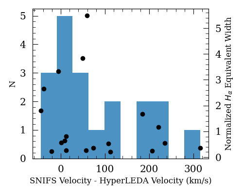
Figure 5: We compare the differences between our measured SNIFS velocities and HyperLEDA’s aggregated velocities, finding two distinct groups. The 12 galaxies on the left side of the histogram have an average difference of 27 km s^-1 and a standard deviation of 48 km s^-1. The 4 galaxies on the right are offset by several hundred km s^-1. Three of the four HyperLEDA velocities come from relatively older sources, and could be the result of inaccurate methodologies. Each galaxy in the histogram also has a marker with a y-value corresponding to its rescaled H_α equivalent width. The presence of weak equivalent widths in the sample with low velocity differences suggests that the four discrepancies are not due to weak spectral features.

Figure 6: The normalized histograms of targets from SNIFS, FOCAS, and literature in z show distinct redshift distributions. Each galaxy’s Pan-STARRS $g$ Kron mag is plotted against redshift to show that the distribution in magnitudes are also distinct. Triggering only on transients in galaxies with redshifts in the literature biases the sample towards lower redshifts and brighter galaxies. By triggering on galaxies regardless of redshift availability, we mitigate this issue.

We note that galaxies in larger groups will have an additional velocity term due to intracluster dynamics, and that using the group redshift would likely probe large-scale flows more robustly, as done in Peterson et al. (2022). However, pursuing spectroscopic observations for all members of an associated group would reduce the number of SNe Ia host galaxies we could observe. We note that our analysis will benefit from future large spectroscopic surveys such as DESI (Collaboration et al., 2022).

All redshift uncertainties are converted to uncertainties in distance modulus via the distance-redshift relation for an empty universe presented in Kessler et al. (2009):

$$\sigma^{z}_{\mu}=\sigma_{z}\left(\frac{5}{\ln{10}}\right)\frac{1+z}{z(1+z/2)}.$$ (3)

Different cosmological models produce negligible differences in $\sigma^{z}_{\mu}$, which is already subdominant compared to other sources of uncertainty in the distance modulus.

3 Distance Determination

In this section, we describe the specific methodology used to convert our data into distance moduli using SNooPy and SALT3-NIR as they were the only publicly available fitting programs that can utilize optical and NIR observations when our analyses began. We only intend to describe our fitting procedures to contextualize the results presented in section 6, and as such we will not be claiming one program is more accurate or more appropriate for our use case. We leave such an analysis for future work, where we will also incorporate fits from BayeSN, which was made public with Mandel et al. (2022), and has been updated with Grayling et al. (2024).

3.1 SNooPy

SNooPy is a Python package designed for fitting light-curves of SNe Ia from the Carnegie Supernova Project (CSP; Contreras et al., 2010; Burns et al., 2011). It estimates luminosity distances by comparing data spanning flux, phase, and a shape parameter to filter-specific three-dimensional models (Burns et al., 2011). These models were produced using high-cadence observations of SNe Ia in the CSP photometric system (Hamuy et al., 2006). We use version 2.5.3, which does not yet include the improved models of Lu et al. (2023). We look forward to reprocessing our sample when SNooPy incorporates these templates.

Using SNooPy to calculate distance moduli involves several non-trivial decisions. SNooPy offers two distinct ways to characterize the shape of a SN Ia light-curve; one being the decline rate parameter ($\Delta m_{15}$; Phillips et al., 1999), and the other being the colour-stretch parameter (s_BV; Burns et al., 2014). The latter is less sensitive to changes in reddening (varying $\sim 1$% across A_V = 3 mag) and does not become degenerate for fast-declining SNe Ia ($s_{BV}<0.7$), as seen with $\Delta m_{15}$ (Burns et al., 2014). As such, we use $s_{BV}$ when characterizing light curves with SNooPy.

As an additional decision point, SNooPy offers two models that allow for varying levels of assumptions when fitting SNe Ia light curves. EBV_model2 uses light curves in numerous filters to infer four global parameters: the shape ($\Delta m_{15}$ or $s_{BV}$), the time of B-band maximum, extinction from the host galaxy, and distance modulus. The model has been calibrated multiple times using various subsets of 36 SNe Ia as described in Folatelli et al. (2010), with the default calibration using the 21 best-observed SNe Ia, excluding the heavily reddened SN 2005A and SN 2006X. The max_model relaxes the requirement that multiple bandpasses follow a well-characterized reddening law, and fits for the peak apparent magnitude in each filter, a global shape parameter, and the time of B-band maximum. Distance moduli can be calculated based on each apparent maximum using the formulae presented in Burns et al. (2018), which were produced from 137 SNe Ia and include 19 SNe Ia in galaxies with Cepheid-based distance measurements, or by formulae derived in the same manner. We use Stan (Carpenter et al., 2017) to infer the nuisance parameters $P_{0}$, $P_{1}$, $P_{2}$, and $\beta_{max}$ in the equation

$$m_{X}=P_{0}+P_{1}(s_{BV}-1)+P_{2}(s_{BV}-1)^{2}+\mu_{\mathrm{cos}}+\beta_{max}(m_{Y}-m_{Z})$$ (4)

where $m_{X}$, $m_{Y}$, and $m_{Z}$ are the peak apparent magnitudes determined by the max_model fit in the bandpasses $X$, $Y$, and $Z$ (these arbitrary labels are not to be confused with the $Y$ or $Z$ bandpasses). We omit the term correlating luminosity and host-galaxy mass to maintain consistency with EBV_model2, which does not factor in galaxy mass.

All models account for Galactic extinction using dust maps from Schlafly & Finkbeiner (2011). Recent work has made use of both the EBV_model2 (Phillips et al., 2022; Jones et al., 2022; Pierel et al., 2022; Peterson et al., 2023) and the max_model (Burns et al., 2018; Phillips et al., 2022; Uddin et al., 2023; Lu et al., 2023), so we fit each SN with both models to produce two samples.

3.1.1 Estimating Uncertainties

SNooPy provides estimates of statistical uncertainty in all inferred parameters following either frequentist or Bayesian conventions. Initial fits without priors produce statistical errors using the standard frequentist convention of inverting the Hessian matrix at the best-fitting parameters to produce a covariance matrix. When this matrix is singular, as can happen with undersampled light curves or for light curves of non-SNe Ia, the model becomes insensitive to one or more parameters and will not infer values for any of them. After the initial fit, SNooPy offers a Markov chain Monte Carlo (MCMC) method which samples their posterior distributions with the package emcee (Foreman-Mackey et al., 2013). The default priors are based on previous work with the CSP sample, but can be overwritten with arbitrary functions.

In addition to providing statistical errors, SNooPy provides an uncertainty floor for each parameter. The floor in the distance modulus reflects the uncertainty in the various terms used to standardize SNe Ia luminosities. These terms depend on the model used, but generally include filter-specific measurements of peak absolute magnitude and how that changes with $s_{BV}$. Thus, the distance modulus accuracy has a systematic floor determined by the sample used to calibrate it and becomes less accurate as the shape factor deviates from its normal value. The other floors have constant values derived from various analyses. The uncertainty floor in $s_{BV}$ is 0.03, and comes from the dispersion around a quadratic fit of $s_{BV}$ to the SALT $x_{1}$ parameter (discussed in section 3.2) (Burns et al., 2014). The host galaxy extinction floor is 0.06 mag, coming from the intrinsic dispersion of the $B-V$ colours in the CSP sample after correcting for reddening. In the max_model, the peak magnitudes in each bandpass are presented with uncertainty floors based on Folatelli et al. (2010). Lastly, the time of B-band maximum is fixed to have an uncertainty floor of 0.34 days. We define the uncertainty on each parameter estimate as the quadrature sum of the statistical uncertainty and the floor.

3.1.2 K- and S-corrections

Observations of SNe Ia at significant redshift can lead to a mismatch between the observed and rest-frame spectral energy distribution (SEDs). One could almost trivially account for this issue in spectral observations if the redshift is known (telluric corrections aside), but photometric observations require some knowledge of the underlying SED to determine what is shifted into and out of the effective bandpass. The adjustments needed to compensate for the mismatches between observed and emitted SEDs are called “K-corrections” (Humason et al., 1956; Oke & Sandage, 1968).

Similarly, variations in an optical system’s transmission function leads to differences in instrumental magnitudes that depend on the SED observed. SNooPy models are defined in the CSP photometric system, and using data from other bandpasses would introduce systematic errors in the parameter inferences. The typical treatment for managing multiple filter sets is to observe a range of standard stars and perform linear fits of colour terms to transform one set to the other. Using stellar standards produces equations capable of converting stellar observations between filter sets, but SNe Ia have non-stellar SEDs, and there are no perennially available standard SNe Ia. The solution is to apply an “S-correction” (Burns et al., 2011).

SNooPy applies both of these corrections simultaneously by calculating a “cross-band K-correction” (Kim et al., 1996) using the spectral library from Hsiao et al. (2007), which combines $\sim 600$ heterogeneous spectra of $\sim 100$ SNe Ia. Although the library covers a wide breadth, the available spectra cannot represent every kind of SN Ia at every possible epoch. To account for levels of reddening and intrinsic colours not seen in the spectral library, Hsiao et al. (2007) describe a “mangling” process by which template spectra can be multiplied by a smoothly varying spline to match observed colours. The statistical error on each K-correction and mangling varies between about 0.01 mag and 0.04 mag depending the amount of overlap between the redshifted rest-frame CSP bandpass and the observed bandpass. Pairs with little overlap rely on extrapolation, and are more sensitive to the spectral template used (Hsiao et al., 2007), whereas a rest-frame bandpass that maps exactly on to an observed bandpass would be completely insensitive to the underlying spectrum. The ATLAS $c$ and $o$ bandpasses are wider than those in the CSP photometric system, and so they necessarily belong to the former category.

3.2 SALT

SALT fits SNe Ia light-curves using a different approach (Guy et al., 2005, 2007, 2010). Roughly speaking, where SNooPy attempts to fit observed light curves to well studied light curves, SALT attempts to fit observed light curves to a spectral time series. This model is built from a term that describes the phase-independent effect of the colour law ($CL(\lambda)$) and two or more surfaces spanning flux, phase ($p$), and wavelength ($\lambda$), whose combinations describe the spectral flux and evolution of all SNe Ia:

$$F(p,\lambda)=x_{0}[M_{0}(p,\lambda)+x_{1}M_{1}(p,\lambda)+...]\times\exp{[c\times CL(\lambda)]},$$ (5)

where $M_{i}$ is the $i$th surface, $x_{i}$ scales how much that surface contributes to the spectral flux, and $c$ scales the colour law (Guy et al., 2007). The surfaces are empirically derived, with $M_{0}$ encapsulating the ‘standard’ SN Ia spectral time series while the remaining surfaces describe all other modes of variation. This means the surfaces themselves may not correlate exactly with the physical parameters of SNe Ia, but instead may be understood as principal components. With that said, $x_{1}$ is often considered a shape factor like $s_{BV}$ or $\Delta m_{15}$ since light-curve shape seems to be the dominant mode of variation. Each combination of $x$ terms defines a SED and evolution that can be further sculpted by $c$, the colour law, and redshift. At any observational epoch, a filter set’s transmission functions is used to make synthetic magnitudes which can be compared to real photometry. Thus one can infer the most likely SALT parameters and their uncertainties given observations of a particular SN Ia. These parameters provide a distance modulus ($\mu$) by the equation

$$\mu=m^{*}_{B}-M+\alpha x_{1}-\beta c,$$ (6)

where $m^{*}_{B}$ is the rest-frame Bessell $B$-band magnitude (Perlmutter et al., 1997), $M$ is the absolute magnitude of a SN Ia with $x_{1}=c=0$, and $\alpha$ and $\beta$ are standardization coefficients. While $m^{*}_{B}$ can be approximated by $-2.5\log_{10}(x_{0})+\text{const.}$, we calculate its value using synthetic photometry based on model parameters.

Rubin (2020) suggested that SNe Ia luminosity variability may consist of three to five independent parameters. Attempts to standardize SNe Ia luminosities using one or two parameters report an “intrinsic scatter” that cannot be explained by measurement error alone (e.g. Scolnic et al., 2018; Brout et al., 2022). Rose et al. (2020) explored the differences between two and seven-component fits using SNEMO (Saunders et al., 2018), and found that only CSP data had the SNR and coverage to constrain the additional parameters. Put another way, a two-component fit with SALT compares to a seven-component fit with SNEMO for all but the most extensively covered light curves. With that in mind, we use the two-component fits of SALT3-NIR (Pierel et al., 2022). The only other SALT model that can process NIR light-curves is SALT2-Extended, but it was trained on optical data extrapolated to the NIR and is thus insensitive to correlations between SALT parameters and NIR light-curve properties (Pierel et al., 2018). SALT3-NIR was jointly trained on the optical sample of 1083 SNe Ia from Kenworthy et al. (2021) and 166 SNe Ia with NIR data (Pierel et al., 2022). We access the SALT3-NIR model through the Python package SNCosmo version 2.9.0 (Barbary et al., 2022), and utilize the convenience functions therein to account for Galactic extinction using the dust maps of Schlafly & Finkbeiner (2011) and the dust model from Fitzpatrick (1999) with $R_{V}=3.1$. Notably, we use SNCosmo to calculate model fluxes given a set of SN Ia parameters, but do not use the built-in functions to estimate those parameters. Instead, we use the fitting methodology of Rubin et al. (2023), defining a $\chi^{2}$ function and using a downhill-simplex algorithm to iteratively identify the SALT parameters that minimize that function.

3.2.1 Estimating Uncertainties

The covariance matrices we obtain for each object’s best-fitting SALT parameters (time of $B$-band maximum light, $x_{0}$, $x_{1}$, and $c$) reflect three sources of uncertainty. Our NIR photometric methods produce correlation matrices, but we assume the measurements and errors from ATLAS, ASAS-SN, and ZTF are completely independent. We incorporate the SALT3-NIR model uncertainties during our fitting process. Lastly, we repeat each fit with slightly varied inputs to calculate derivatives between the fitting parameters and quantities like redshift, Galactic extinction, and the photometric zero-point in each bandpass.

The error explicitly associated with K-corrections and S-corrections is ostensibly removed due to SALT’s use of spectra when fitting. However, if the intrinsic SED of a SN Ia differs from the form of Equation 5 truncated after $i=1$, the synthetic photometry will be inaccurate. We assume these errors are encapsulated in the model uncertainties.

The distance modulus in Equation 6 requires specifying the standardization coefficients $\alpha$ and $\beta$, which are typically calibrated empirically. Fitting for $\alpha$ and $\beta$ by minimizing dispersion in the Hubble residuals introduces a form of Eddington bias due to uncertainties in $x_{1}$ and $c$. We estimate the standardization coefficients using a Bayesian framework called UNITY (Unified Nonlinear Inference for Type-Ia cosmologY; Rubin et al., 2015, 2023). UNITY assumes a Gaussian and skew normal distribution for the population distributions of the true value of each SN’s $x_{1}$ and $c$ respectively, and uses flat hyperpriors for the means of each distribution and the log of their standard deviations. This approach avoids Eddington bias, which would suppress both coefficients. Although UNITY can model $\alpha$ and $\beta$ as broken-linear functions, we assume the coefficients are constants. In Section 6.2 we identify and discuss a systematic issue tied to this decision.

4 Validating Data and Methodology

In this section, we validate our data reduction and modelling techniques by partially reproducing the analysis of the DEHVILS survey (Peterson et al., 2023) using our NIR photometry and fitting methodologies. To evaluate the differences produced by these variations, we compare each inferred distance modulus ($\mu_{\mathrm{fit}}$) and the theoretical distance modulus at its corresponding redshift in a fiducial cosmology ($\mu_{\mathrm{cos}}$). These Hubble residuals are calculated as

$$\Delta\mu =\mu_{\mathrm{fit}}-\mu_{\mathrm{cos}}$$ (7)

$$\mu_{\mathrm{cos}} =5\log_{10}\Big{[}\Big{(}\frac{cz_{\mathrm{CMB}}}{H_{0}}\Big{)}\Big{(}\frac{1+z_{\mathrm{hel}}}{1+z_{\mathrm{CMB}}}\Big{)}\Big{(}1+\frac{1-q_{0}}{2}z_{\mathrm{CMB}}\Big{)}\Big{]}-25,$$ (8)

where $H_{0}$ is the Hubble constant and $q_{0}$ is the cosmic deceleration parameter, which we take as $-0.53$ (Planck Collaboration et al., 2020). As stated in Burns et al. (2018), the factor of $(1+z_{\text{hel}})/(1+z_{\text{CMB}})$ accounts for observational effects which should be corrected in a heliocentric rest-frame. In each sample we define $H_{0}$ such that the inverse-variance weighted average of the Hubble residuals is 0 mag.

The dispersion in $\Delta\mu$ is typically characterized through RMS (e.g. Blondin et al., 2011; Avelino et al., 2019; Foley et al., 2017; Jones et al., 2022; Pierel et al., 2022; Peterson et al., 2023); inverse-variance weighted RMS (WRMS; e.g. Blondin et al., 2011; Avelino et al., 2019; Foley et al., 2017), or normalized median absolute deviation (NMAD; e.g. Boone et al., 2021; Peterson et al., 2023). SNe Ia analyses repeatedly find that measurement uncertainty alone cannot explain the observed dispersion, indicating that SNe Ia luminosities include some unmodelled variance commonly called intrinsic scatter ($\sigma_{\text{int}}$; e.g. Blondin et al., 2011; Scolnic et al., 2018; Burns et al., 2018).

Lastly, we validate our treatment of max_model parameters by using photometry from CSP-I DR3 Krisciunas et al. (2017) to re-derive the Tripp calibration parameters in Table 1 of Burns et al. (2018). We comment on the unique sensitivity of the max_model to certain spectral subtypes of SNe Ia.

4.1 Comparisons with DEHVILS

The DEHVILS survey collected data in tandem with Hawai‘i Supernova Flows, also using UKIRT’s WFCAM to collect NIR observations of SNe Ia (Peterson et al., 2023). Our programs differ in that DEHVILS collected photometry in the $Y$-, $J$-, and $H$-bands and pursued more observations (median 6 epochs per bandpass) for fewer SNe ($N=96$). We shared $J$-band observations near peak to avoid redundancy, but reduced the data through independent photometric pipelines. Given light curves of 96 SNe Ia, roughly half are eliminated by quality cuts. The DEHVILS cuts are $|x_{1}|<3$, $\sigma_{x_{1}}<1$, $\sigma_{t_{0}}<2$, $E(B-V)_{\text{MW}}<0.2$ mag, and a Type Ia LC fit probability defined in SNANA $P_{\text{fit}}>0.01$. $\sigma_{x_{1}}$ and $\sigma_{t_{0}}$ refer to the uncertainty in the SALT parameter $x_{1}$ and the estimated time of maximum light. We assume the parameters used for the cuts are the ones presented in Table 5, “Optical-only SALT3 fit results” (Peterson et al., 2023). We apply the first four cuts trivially, but $P_{fit}$ is a parameter from SNANA and is undefined with our methods. Worse, this last cut is responsible for 40 of the 46 SNe removed in Peterson et al. (2023), and cannot be ignored. Given that SNANA obtains parameter values by minimizing the data-model $\chi^{2}$, we emulate the $P_{fit}$ cut by fitting DEHVILS and ATLAS photometry using SALT3-NIR and determining the minimum reduced $\chi^{2}$ per degree of freedom (DoF) cut value that produces a sample of 47 objects: $\chi^{2}/\text{DoF}\leq 6.66$. We note that our $\chi^{2}$ function includes model covariances.

4.1.1 Varying Fitting Methodology

To isolate the effects of the difference in our methodologies we use DEHVILS photometric measurements for all NIR data and fit the sample with SNooPy’s EBV_model2, SNooPy’s max_model, and SALT3-NIR using the bandpass combinations $co$, $coYJH$ and $YJH$ for all three fitters. By Equation 4, calculating distance moduli using the max_model requires specifying a bandpass ($m_{X}$) and a colour ($m_{Y}-m_{Z}$), which makes comparisons between max_model fits subject to systematic discrepancies when the bandpasses differ. There is no bandpass and colour common to the bandpass combinations we examine, but we may still compare each implementation of the max_model against the DEHVILS results. For the $co$ combination, we use the $V$ bandpass and the $V-r$ colour; for $coYJH$, we use $J$ and $V-r$; and for $YJH$, we use $J$ and $Y-J$. We calculate SALT-based distance moduli using $\alpha$ and $\beta$ parameters derived with UNITY (Rubin et al., 2015), except for the $YJH$ sample which encountered numerous problems during modelling and produced an anomalously low and noisy $\beta=1.14\pm 1.26$. For this sample we calculate the values that minimize the standard deviation of the Hubble residuals. The standardization coefficients for the $co$, $coYJH$, and $YJH$ samples are ($\alpha$, $\beta$) = (0.155, 3.3), (0.138, 3.702), and (0.111, 2.475) respectively. For comparison, Peterson et al. (2023) used standardization coefficients of ($\alpha$, $\beta$) = (0.145, 2.359) and (0.075, 2.903) for the $co$ and $coYJH$ samples, with no standardization applied to the $YJH$ sample. They characterize the dispersion in Hubble residuals using NMAD and standard deviation (STD), so we use the same statistics in this section.

Our methods noticeably differ in fitting one of the bandpass combinations. In the DEHVILS analysis, the fit parameters $x_{1}$ and $c$ were held fixed at 0 for the NIR-only sample. Our methodology does not hold these parameters fixed, and we found greater dispersion. This is consistent with their finding that keeping $c$ constant while allowing $x_{1}$ to vary led to increased scatter. For the other $co$ bandpass combination, we found dispersions in Hubble residuals roughly consistent with the DEHVILS values and errors presented in Peterson et al. (2023) and reproduced in Table 2. Our NMAD values were lower and our STD values higher, implying our Hubble residuals are heavier-tailed than a Gaussian distribution. This could be an effect of different sample selection, different treatment of ATLAS photometry, or different standardization coefficients. For the $coYJH$ bandpass combination, our analysis with SNooPy’s EBV_model2 is consistent with the DEHVILS values, but the other two models tend to produce higher dispersion values. We note that in our SALT3-NIR analysis, if we use the $\alpha$ and $\beta$ values that minimize NMAD (0.100 and 3.052 respectively), we find a value of 0.124 mag and an STD of 0.162 mag, which is consistent with the DEHVILS values. Our max_model analysis is also not optimized against dispersion. We use the $J$-band peak magnitude and $V-r$ pseudo-colour to infer distances because that is the methodology we apply to our own photometry, which does not include $Y$- or $H$-band observations.

The consistency between the dispersion values we measure and the values reported in Peterson et al. (2023) suggests that our methodology is comparable for fits when using optical data or optical and NIR data. Our methodology is inferior for fits using only NIR photometry, and max_model fits using $coYJH$ photometry, indicating that we would need to adapt our methodology if we were to collect $Y$- and $H$-band data like the DEHVILS team and produce NIR-only samples. The samples we produce using our own $J$-band data always include optical data.

Given that our $P_{fit}$ cut was approximate, the samples are distinct from the one analysed in Peterson et al. (2023). However, the effects of a few mismatched SNe should be suppressed after bootstrap resampling the Hubble residuals. As in the DEHVILS analysis, we use 5,000 iterations and estimate the uncertainty of the dispersion with the standard deviation of resampled measurements.

Model	Filters	N	NMAD (mag)	STD (mag)
DEHVILS	co	47	$0.177(029)$	$0.221(043)$
DEHVILS	coYJH	47	$0.132(025)$	$0.175(034)$
DEHVILS	YJH	47	$0.139(026)$	$0.172(027)$
EBV_model2	co	50	$0.148(028)$	$0.245(044)$
EBV_model2	coYJH	50	$0.119(021)$	$0.163(031)$
EBV_model2	YJH	47	$0.179(049)$	$0.239(033)$
max_model	co	52	$0.171(028)$	$0.300(055)$
max_model	coYJH	52	$0.168(027)$	$0.245(051)$
max_model	YJH	49	$0.215(052)$	$0.462(112)$
SALT3-NIR	co	47	$0.153(032)$	$0.272(047)$
SALT3-NIR	coYJH	47	$0.191(032)$	$0.196(022)$
SALT3-NIR	YJH	46	$0.178(035)$	$0.300(088)$

Table 2: We highlight any differences due to methodology by using DEHVILS photometry and approximating their quality cuts. We did not replicate their findings when using only $YJH$ photometry, which is where our methodologies differ the most. The DEHVILS team fixed $x_{1}$ and $c$ to 0 for those fits and we allowed them to vary. For the $co$ bandpass combination, our methodology produced Hubble residual dispersions consistent with the values reported by DEHVILS. We find mixed results with the $coYJH$ combination, with our max_model analysis producing larger dispersions, and our SALT3-NIR analysis producing consistent results only if we solve for the $\alpha$ and $\beta$ values that minimize dispersion in the Hubble residuals.

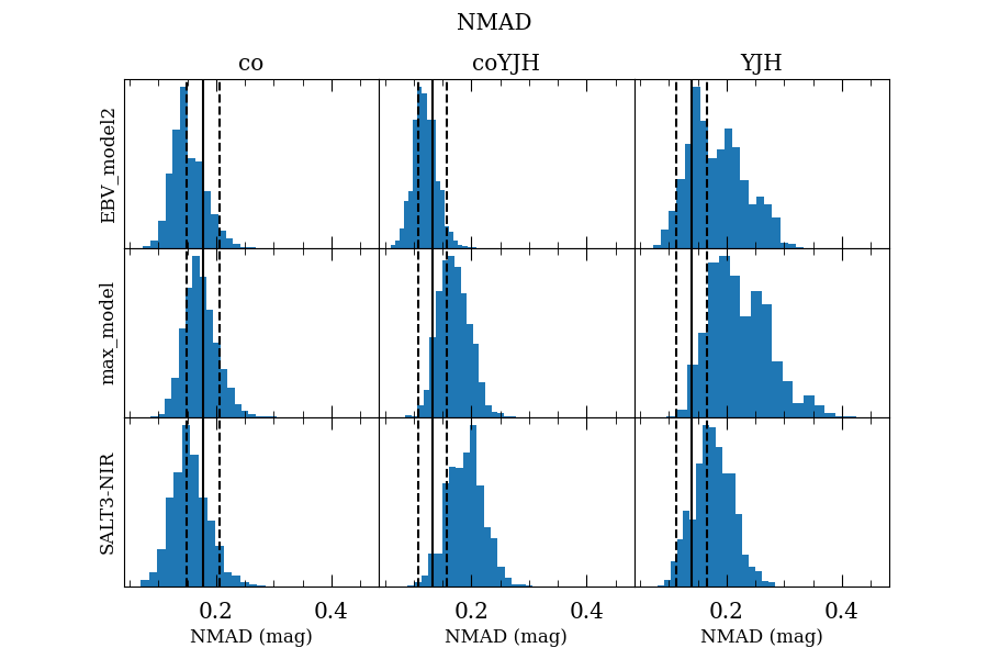
Figure 7: We show the distributions of NMAD in 5,000 bootstrap resamplings of each set of Hubble residuals. The columns correspond to the fitting model used the rows to the bandpass combination. The solid and dashed vertical lines show the values and uncertainties of the NMAD reported in the DEHVILS survey. Our methodology produces Hubble residuals with dispersions consistent with the values reported by the DEHVILS survey using SNooPy’s EBV_model2, but not when using SALT3-NIR or SNooPy’s max_model.

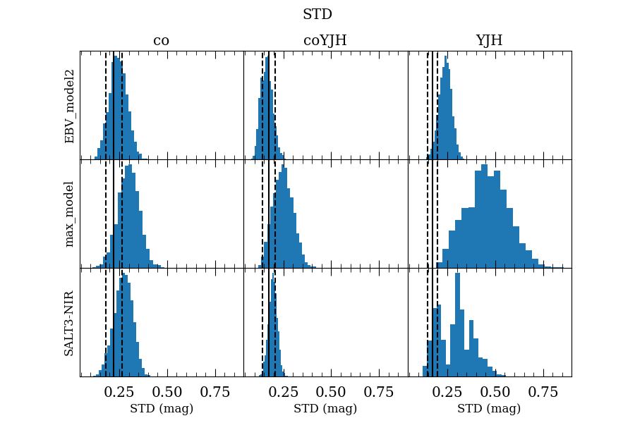
Figure 8: The same set of plots as Figure 7, but showing standard deviation instead of NMAD.

4.1.2 Varying Photometry

We repeat the comparative analysis of the previous section, this time isolating the effects of differing photometry. We fit ATLAS and either our $J$-band data or that of the DEHVILS survey to create two sets of fits for each of our three models. We apply the $\chi^{2}/\text{DoF}\leq 6.66$ based on the greater value between the fits using our photometry or that of DEHVILS. This ensures the two samples for each model use the same SNe.

Once more, we bootstrap resample the Hubble residuals to estimate the uncertainties in our dispersion measurements, but we include an additional set of statistics. When varying methodology, we could only compare the distributions of our resampled dispersion measurements with the values reported in Peterson et al. (2023), but in this analysis we can make pairwise comparisons between individual iterations of the resampling process. For each iteration, we randomly choose SNe Ia with replacement, record the NMAD and STD of their Hubble residuals in our six samples, and additionally calculate the differences in dispersion between each model’s sample using our $J$-band photometry and using DEHVILS photometry ($\Delta D=D_{\textrm{HSF}}-D_{\textrm{DEHVILS}}$ where $D$ is either NMAD or STD). Thus, we not only produce distributions of NMAD and STD, but also distributions of $\Delta$NMAD and $\Delta$STD.

The averages and standard deviations of these values are presented in Table 3 and the histograms of dispersions and differences are plotted in Figure 9. None of the distributions indicate that using our photometry instead of DEHVILS photometry leads to increased dispersion measurements. The averages are within one standard deviation of each other, and the differences within one standard deviation of no change in dispersion.

Model	$J$ Data	N	NMAD (mag)	STD (mag)
EBV_model2	HSF	39	$0.134(027)$	$0.136(015)$
EBV_model2	DEHVILS	39	$0.130(032)$	$0.143(016)$
max_model	HSF	40	$0.110(030)$	$0.147(019)$
max_model	DEHVILS	40	$0.123(025)$	$0.132(014)$
SALT3-NIR	HSF	21	$0.132(068)$	$0.190(034)$
SALT3-NIR	DEHVILS	21	$0.192(065)$	$0.190(034)$

Table 3: We use our methodology to calculate Hubble residuals using ATLAS photometry and either our $J$-band photometry or that of the DEHVILS survey. Bootstrap resampling these residuals 5,000 times shows the dispersion measurements are insensitive to any differences between our photometry. In SNooPy’s EBV_model2 and max_model and in SALT3-NIR, the change in dispersion is consistent with 0.

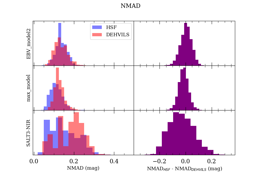
Figure 9: The blue and red histograms show the distributions of NMAD dispersion measurements after 5,000 iterations of bootstrap resampling Hubble residuals. The purple histograms show the distributions of differences in dispersion between the samples using HSF photometry and the samples using DEHVILS photometry in each iteration. Using our measurements instead of DEHVILS photometry may lead to a decrease in the dispersion of the Hubble residuals, but it is not statistically significant.

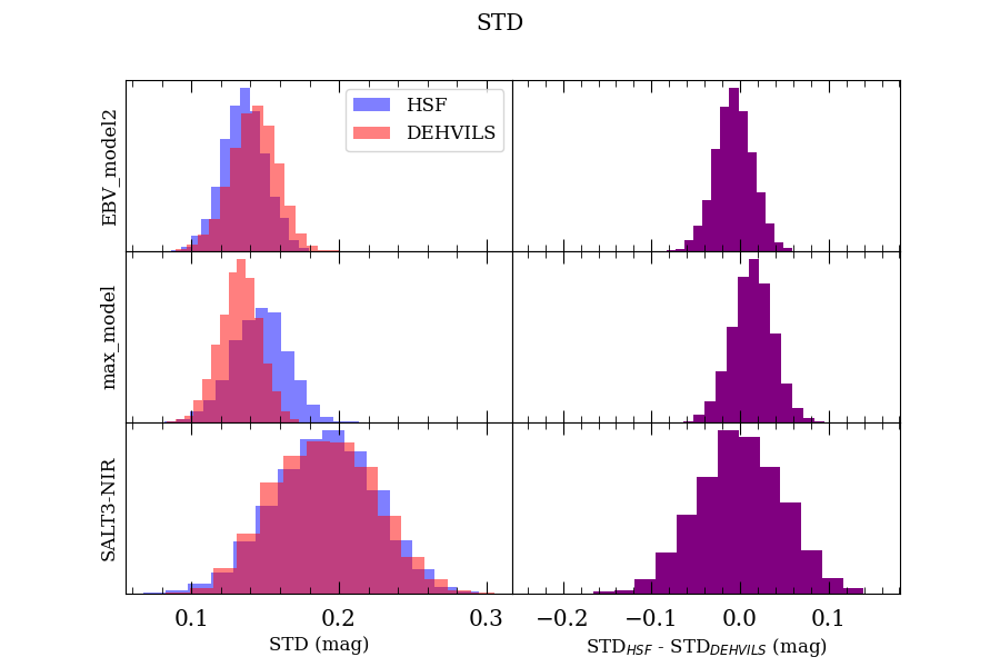
Figure 10: The same set of histograms as Figure 9, but applied to standard deviation rather than NMAD. Again, using our measurements instead of DEHVILS photometry does not lead to a statistically significant difference in the dispersion of the Hubble residuals. The closest case is the standard deviation in the max_model, which increases by an average of $0.014\pm 0.022$ mag. The more robust NMAD decreases by $0.015\pm 0.038$ mag, indicating the increase in standard deviation is due to a few discrepant values rather than a systematically preferred set of photometry.

4.2 Comparison with CSP

The EBV_model2 produces Hubble residuals with lower dispersion than those produced by either SALT3-NIR or the max_model. The greater dispersion in the max_model was unexpected since the EBV_model2 is calibrated to CSP observations of 36 SNe, whereas in this analysis we derived standardization coefficients for the max_model using our observations of 52 SNe.

4.2.1 Validating Tripp Calibration

To test our derivation process, we used photometry from CSP-I DR3 (Krisciunas et al., 2017) to solve for the calibration coefficients presented in Table 1 of Burns et al. (2018). We fit all CSP photometry with the SNooPy max_model, parametrizing light-curve shape with $s_{BV}$. We use the heliocentric redshifts provided in the data release rather than redshifts from HyperLEDA to focus on differences due to methodology. Our Equation 4 does not include a term for host-galaxy mass, but in order to match the CSP derivation methodology we reintroduce this term:

$$\begin{split}m_{X}=&P_{0}+P_{1}(s_{BV}-1)+P_{2}(s_{BV}-1)^{2}+\mu_{\mathrm{cos}}\\ &+\beta_{\mathrm{max}}(m_{Y}-m_{Z})+\alpha_{\mathrm{M}}\left(\log\left(M_{\ast}/M_{\odot}\right)-M_{0}\right)\end{split}$$ (9)

Where $\alpha_{\text{M}}$ is the coefficient correlating magnitude and host-galaxy stellar mass ($M_{\ast}$) and $M_{0}$ is an arbitrary mass zero point, taken as $10^{11}M_{\odot}$. We follow the methodology in Appendix B of Burns et al. (2018) for assembling host-galaxy stellar masses, primarily drawing from the 2MASS Extended Source Catalog (Jarrett et al., 2000), which we convert from $K$-band apparent magnitudes to stellar masses assuming a constant mass-to-light ratio.

$$\log_{10}\left(M_{\ast}/M_{\odot}\right)=-0.4\left(m_{K}+\mu\right)+C$$ (10)

where $\mu$ is the distance modulus and $C$ is a constant which CSP determined to be 1.04 dex by comparing masses from the 2MASS catalogue with mass estimates from Neill et al. (2009). We verify that this is the best-fitting value from a simple least-squares regression. When there is no $K$-band magnitude available, we use estimates from Neill et al. (2009) and Chang et al. (2015) when possible, as Burns et al. (2018) did.

The coefficients in Equation 4 derived in Burns et al. (2018) and re-derived with our methods are presented in Table 4. The average deviation between the two sets of coefficients is 0.623 times the quadrature sum of the uncertainties. Additionally, we derive a set of coefficients while not accounting for host-galaxy mass. As expected, the average difference between this set and the original values is greater, albeit only slightly at 0.720 times the combined uncertainty.

Derivation	$P_{0}$	$P_{1}$	$P_{2}$	$\beta_{\mathrm{max}}$	$\alpha_{\mathrm{gal}}$	$\sigma_{\mathrm{int}}$	$v_{\mathrm{pec}}$
	(mag)	(mag)	(mag)		(mag/dex)	(mag)	(km s-1)
CSP	-18.633(062)	-0.37(12)	0.61(32)	0.36(10)	-0.056(029)	0.11	336
This Work	-18.611(028)	-0.328(130)	0.032(413)	0.309(094)	-0.046(031)	0.060(032)	363(52)
This Work (No Masses)	-18.589(025)	-0.281(133)	0.088(432)	0.289(096)	N/A	0.072(033)	363(52)

Table 4: We show some of the Tripp calibration coefficients presented in Table 1 of Burns et al. (2018) and our derivations using the same data with our methodology. Our values differ from the original values by an average of 0.623 times the combined uncertainty. When not accounting for host-galaxy masses, the average difference slightly increases to 0.720 times the combined uncertainty.

We conclude that our methodology for calibrating the Tripp method is consistent with the method used in Burns et al. (2018). The difference in dispersion in Hubble residuals between the max_model and EBV_model2 seen in Section 4.1.1 is not due to errors in determining the calibration coefficients. Additionally, we do not find a significant difference in dispersion between the two models when examining the CSP data. Using the max_model, the Hubble residuals have a NMAD dispersion of 0.163 mag and a standard deviation of 0.233 mag, which is only marginally greater than the same values using EBV_model2: 0.157 mag and 0.227 mag.

5 Sample Selection

We have NIR observations of 1218 unique transients, but only about a quarter of those are presently useful for cosmology. Our final sample is comprised of targets that pass three sets of cuts: one based on observational data, one based on fitting parameters, and one based on several outlier detection algorithms. The number of targets discarded and remaining after each cut are presented in Tables 5 and 6.

5.1 First Cut: Observational Data

The set of all our observed transients includes unclassified or misclassified non-SNe Ia, galaxies with photometric or unknown redshifts, and SNe Ia missing coverage near maximum light in one or more all-sky survey bandpasses. In future work we intend to incorporate the unclassified transients that are photometrically consistent with SN Ia light curves, but for this paper, we do not include them in our analysis.

Of the 1218 observed transients, 669 have been spectroscopically classified as usable SNe Ia. This number does not include SNe Ia subtypes that are unsuitable for distance inference using SALT3-NIR or SNooPy: 2002cx-like SNe (sometimes called SNe Iax, Li et al., 2003), 2002ic-like SNe (sometimes called SNe Ia-CSM, Hamuy et al., 2003), 2003fg-like SNe (formerly called super-Chandrasekhar SNe or SNe Ia-SC, Howell et al., 2006; Hicken et al., 2007; Ashall et al., 2021), and generally peculiar SNe Ia (Ia-pec). This number does include several 2006bt-like candidates, which we discuss in Section 5.3.

Spectroscopic host-galaxy redshifts are available or have been successfully measured for 600 of these 669 SNe Ia. The remaining 69 include galaxies scheduled for spectroscopic observation, galaxies with spectral features manually judged to be too weak for accurate redshift determination, and galaxies with exceptionally low surface brightness, such that spectroscopic observation is prohibitively expensive. We remove an additional 8 targets that have Galactic reddening greater than 0.3 mag according to Schlafly & Finkbeiner (2011). As the last cut in this set, we remove targets with fewer than 5 optical and NIR observations, counting each quartet of ATLAS exposures as a single observation. Of the remaining 592 SNe Ia, 95 are in galaxies for which we have unreduced spectroscopic observations, and 56 encountered errors during photometric analysis, leaving 441 SNe Ia.

5.2 Second Cut: Fitting Parameters

Removing targets based on fitting parameters necessarily requires successfully running each model’s fitting procedure, which is not guaranteed for each possible permutation of input data. Without sufficient phase coverage in photometry, the shape parameter of a SN Ia becomes underconstrained. The same is true for insufficient wavelength coverage and the colour parameter or host-galaxy extinction. These produce singular covariance matrices, indicating degeneracy in the fitting parameters. Additionally, the models span finite combinations of phase and wavelength, making comparisons to some observations interpolative at best and often times extrapolative. The fit is unsuccessful if all data in a given bandpass lie outside the model domain. However, the phase of any observation is dependent on the estimated time of maximum light, which itself is a fitting parameter. This means that the success of a fit is partially dependent on how the fitting parameters are initialized. When a fit fails because one of the bandpasses has no data in a model’s domain, we attempt to perform the same fit without data from the behaviour bandpass. If that succeeds, we use those fitting parameters to initialize a new fit, reintroducing the excluded data. Sometimes this leads to a successful fit using all available bandpasses, at other times a subset of available bandpasses, and occasionally the fit cannot be salvaged. The success or failure of a fit acts as a cut. We now define three distinct samples based on the three fitting models: SNPY_EBV with 440 fits from SNooPy’s EBV_model2, SNPY_Max with 440 fits from SNooPy’s max_model, and SALT with 441 fits from SALT3-NIR.

After fitting, we apply the following cuts. In the SNPY samples we use quality cuts from Jones et al. (2022), rejecting fits with shape factors outside the interval $0.6<s_{BV}<1.3$ (their “loose” cut) or with uncertainty $\sigma_{s_{BV}}>0.2$, and for SNPY_EBV, rejecting fits with host-galaxy $E(B-V)_{\mathrm{host}}>0.3$. In the SNPY_Max sample, the rest-frame bandpasses used for calculating distances depend on both the observed bandpasses and the redshift. Since we infer distances using the $J$ band and the $V-r$ colour, we cut SNe from SNPY_Max whenever the max_model does not provide inferences for the maximum apparent magnitudes in those bandpasses. While it is possible to force SNooPy to map to these bandpasses, the cross-band K-corrections required become much more sensitive to differences between the assumed and actual SED. This acts as a cut based on redshift. In the SALT sample we reject fits where $|x_{1}|>3$, $\sigma_{x_{1}}>1.5$, $|c|>0.3$, or $\sigma_{c}>0.2$ (Scolnic et al., 2018; Foley et al., 2017; Scolnic et al., 2022). We use the temporal coverage cut from Rubin et al. (2023), which is based on the calculated time of maximum light ($t_{0}$), the phase of the initial observation ($t_{i}$), and the phase of the final observation ($t_{f}$). Given that $t_{0}$ can vary between the three samples, we apply this cut to each sample independently. Adequately observed SNe Ia meet at least one of two sets of criteria. The first set requires $t_{i}$ no more than 2 days after $t_{0}$, $t_{f}$ at least 8 days after $t_{0}$, and $t_{f}-t_{i}$ must span at least 10 days. The second set allows for a later $t_{i}$, up to 6 days after $t_{0}$, as long as $t_{f}-t_{i}$ spans at least 15 days. Lastly, we remove fits with reduced $\chi^{2}$ values above 6.66, which comes from the comparison to the DEHVILS sample in Section 4.1. This leaves our three samples with 347/440 objects in SNPY_EBV, 304/440 in SNPY_Max, and 366/441 in SALT.

5.3 Third Cut: Outlier Detection

There are many vectors for outliers to appear in our sample: spectroscopic misclassification of core-collapse SNe, incorrectly assigned host-galaxy redshifts, errors in photometric reduction, or errors in fitting. Even with ‘perfect’ data and methods, an outlier could arise from anomalous astrophysical properties (e.g. an exotic progenitor system or detonation mechanism) or unclassified Type-Ia peculiarity. In particular, 2006bt-like SNe are difficult to identify without $i$-band or NIR observations (Stritzinger et al., 2011; Phillips, 2012). There are several objects in our sample that are classified as SNe Ia on TNS, but have NIR light-curves suggestive of 2006bt-like SNe: SN 2020naj, SN 2020tkp, SN 2020mbf, and SN 2020sme. We employ two kinds of outlier detection methods. The first compares inferred parameters for common targets between the samples, and the second is based on the mixture model of (Kunz et al., 2007) as implemented through UNITY (Rubin et al., 2015).

5.3.1 Divergent Model Inferences

In a Bayesian framework, the physical parameters inferred by each fitting model should draw from the same posterior distribution of ‘true’ physical parameters. This common quantity allows for simple error detection in the 255 SNe common to all samples. Where the estimates of the same parameter vary significantly, at least one model is likely to have converged on a local maximum in likelihood and is not reliable for inferring other parameters. The top row of Figure 13 shows the relationships between the corresponding fitting parameters in our samples. The SNPY and SALT samples share a common definition for the time of maximum light, but differ in exactly how they quantify light-curve shape and colour. Burns et al. (2018) described a linear transformation between the $x_{1}$ parameter in SALT2 and the $s_{BV}$ parameter in SNooPy. We use orthogonal distance regression and find a slightly different relationship, potentially due to differences between SALT2 and SALT3-NIR. After testing linear, quadratic, and cubic polynomial fits, the Bayesian information criterion marginally favours a linear relationship (269.1, 270.1, 271.5):

$$x_{1}=-0.23(02)+8.02(17)(s_{BV}-1).$$ (11)

Here $s_{BV}$ is the average between the values inferred by SNooPy’s two models. The relationship between $s_{BV}$ values from the two SNooPy models as well as the relationship between their average and the SALT $x_{1}$ parameter is shown in Figure 11.

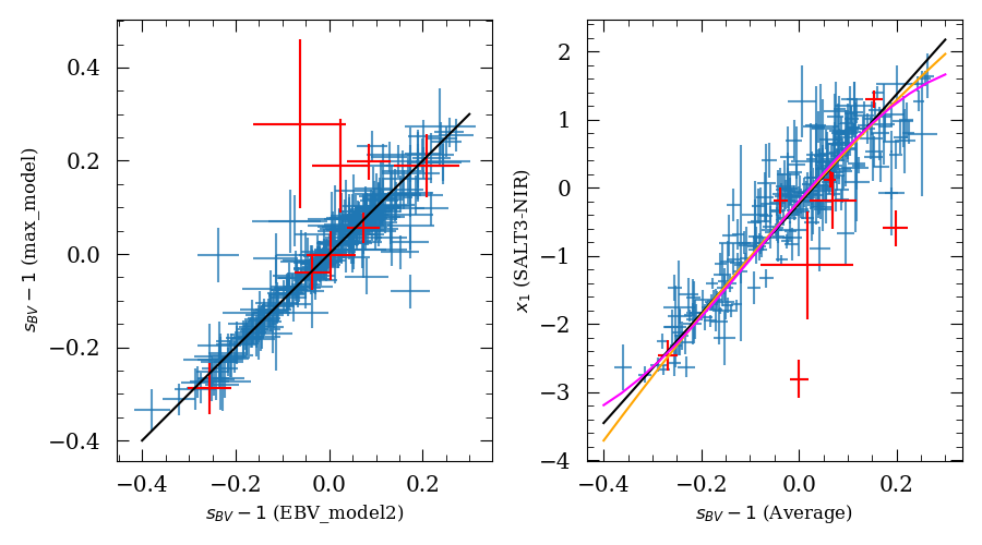
Figure 11: Left: The $s_{BV}$ values of each SN are inferred using the same data, and either SNooPy’s EBV_model2 or max_model. The one-to-one is plotted in black. Right: Each SN’s inverse-variance weighted average $s_{BV}$ value is compared to the $x_{1}$ value inferred by SALT3-NIR. We plot the linear (black), quadratic (orange), and cubic (magenta) polynomial fits determined through orthogonal distance regression. The Bayesian information criterion marginally favours the linear fit. In both plots, we colour outliers identified through divergent model inferences red. These outliers are ignored when calculating the parameter transformation equations.

The $c$ parameter in SALT represents both intrinsic colour variation in SNe Ia and reddening from dust, while the $E(B-V)_{\mathrm{host}}$ fitting parameter in SNooPy is strictly concerned with the latter. However, Brout & Scolnic (2020) found that the correlation between intrinsic colour and luminosity may be weak, and that dust can provide the observed diversity of colours. We test linear, quadratic, and cubic fits, and the Bayesian information criterion again supports a linear fit (-207.3, -201.8, -198.6):

$$c=-0.07(00)+0.98(04)E(B-V)_{\mathrm{host}}\mathrm{mag}^{-1}.$$ (12)

Our colour information in the SNPY_Max sample comes from the differences in apparent maxima. To more effectively parametrize dust, we use the $m_{V}-m_{J}$ pseudo-colour. We test the same polynomial fits, and find support for a cubic fit (427.3, 430.2, 413.4):

$$\begin{split}c=&0.14(01)+0.07(06)(m_{V}-m_{J})\text{ mag}^{-1}\\ &-0.66(14)(m_{V}-m_{J})^{2}\text{ mag}^{-2}\\ &-0.49(09)(m_{V}-m_{J})^{3}\text{ mag}^{-3}\end{split}$$ (13)

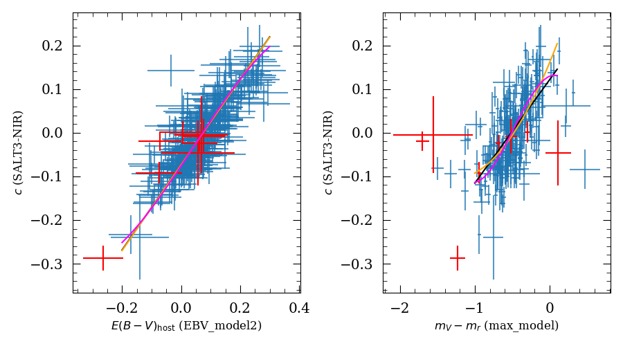
Figure 12: Left: The $E(B-V)_{\mathrm{host}}$ values inferred by SNooPy’s EBV_model2 are plotted against the $c$ values inferred by SALT3-NIR. As in Figure 11, we show the linear (black), quadratic (orange), and cubic (magenta) polynomial fits determined through orthogonal distance regression. The linear and quadratic relationships overlap. Right: For each SN, the pseudo-colour between the peak apparent magnitudes in $V$ and $J$ determined by SNooPy’s max_model are plotted against $c$. Once again, we colour outliers identified through divergent model inferences red. These outliers are ignored when calculating the parameter transformation equations.

After converting the SNooPy parameters into SALT parameters, we can directly compare each model’s inferences for each SN to find where they disagree. We define $\sigma_{t_{0},i}$, $\sigma_{x_{1},i}$, and $\sigma_{c,i}$ as the standard deviation between the transformed fitting parameters of SN $i$ in the SNPY samples its parameters in the SALT sample. We account for correlations between the differences by calculating the Mahalanobis distance between each point $m_{i}=(\sigma_{t_{0},i},\sigma_{x_{1},i},\sigma_{c,i}$) and a distribution $D$ centred at the origin with covariance matrix $\Sigma$ (Mahalanobis, 1930). We approximate $\Sigma$ by bootstrap resampling the parameter differences 5,000 times, calculating each sample covariance $S$, and defining each element $\Sigma_{j,k}$ as the average of all sample elements $S_{j,k}$. Each distance $d_{i}(m_{i},D)=\sqrt{m_{i}\Sigma^{-1}m_{i}^{T}}$, and can be understood as the number of standard deviations between point $m_{i}$ and distribution $D$. The quadrature sum of the standard deviations is a similar metric if all dimensions are normalized to have unit variance, but does not account for correlations. Figure 13 shows the histogram of distances. There are 5 SNe with distances greater than 5 times the standard deviation in $d$, indicating significant disagreement between the models. We recalculated the parameter transformation equations and Mahalanobis distances excluding these 5, and identified no additional outliers. The equations and figures presented are the recalculated versions. Disagreement alone leaves room for one or two of the models to have accurately fit the data, but while manual inspection often reveals which models fit the data well and which do not, we err on the side of caution by removing these 5 SNe from all three samples.

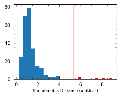
Figure 13: We identify outliers (red) based on disagreement between the three models inferences for a SN’s time of maximum, shape, and colour. After transforming the SNooPy parameters $s_{BV}$, $E(B-V)_{\mathrm{host}}$, and $m_{V}-m_{J}$ to $x_{1}$, $c$, and $c$, we calculate the standard deviations in each SN’s three inferred values for $t_{0}$, $x_{1}$, and $c$. We then parametrize disagreement using the Mahalanobis distance between the standard deviations ($\sigma_{t_{0},i}$, $\sigma_{x_{1},i}$, and $\sigma_{c,i}$) and a distribution centred at the origin. When the three models produce consistent estimates the standard deviation is relatively low, but when they diverge the standard deviation increases.

5.3.2 Mixture-model Analysis

The mixture model introduced as BEAMS (Bayesian Estimate Applied to Multiple Species; Kunz et al., 2007) posits that an imperfect SNe Ia survey will lead to measurements following the sum of multiple distributions. Measurements of real SNe Ia should feature relatively low dispersion whereas measurements of survey contaminants will be more dispersed, and may have a different mean. As implemented in UNITY, both populations are assumed to be Gaussian around a common mean, and the outlier population is assumed to have variances of one in $m^{*}_{B}$, $x_{1}$, and $c$ (Rubin et al., 2015). UNITY’s use of SALT parameters means in its present version it can only process the SALT sample. Since the mixture-model framework is generalizable to arbitrary fitting parameters, future work could allow UNITY to process results from SNooPy. At such a time comparing outliers between samples could indicate whether the SNe Ia is astrophysically exceptional, or whether one of the models is unreliable. For now we are limited to examining SALT.

As UNITY sifts the data through its Bayesian hierarchical model, it produces a population level estimate of the fraction of outliers in the sample (with a prior of $\log{f^{outl}}\sim\mathcal{N}(-3,0.5^{2})$), and a pair of estimates for each object describing the likelihood it belongs to the normal or outlier population. Our sample has an estimated outlier fraction of 0.018$\pm$0.008 and there are 7 SNe more likely to be outliers than a part of the normal population. As before, we take the conservative approach of removing these objects from all samples. Some of the 7 may have been eliminated from the SNPY samples by previous cuts, which is why the number cut at this stage may vary across the samples.

5.4 Final Samples

After all three sets of cuts the sizes of our samples are 338, 294, and 354 for the SNPY_EBV, SNPY_Max, and SALT samples respectively. Tables 5 and 6 enumerate the effect of each cut.

Cuts	Number Cut	Remaining Sample
Spec. Classification	328	890
SN Ia	221	669
Spec. Redshift	69	600
$E(B-V)_{\mathrm{MW}}$ < 0.3	8	592
$N_{obs}\geq 5$	0	592
Successful Spectroscopic Reduction	95	497
Successful Photometric Reduction	56	441

Table 5: Our first set of cuts are independent of the fitting model used and apply to all targets observed.

Cuts	SNPY_EBV Cut	Remaining	SNPY_Max Cut	Remaining	SALT Cut	Remaining
Successful Fit	1	440	1	440	0	441
Rest frame $m_{J}$, $m_{V}$, and $m_{r}$			88	352
0.6 < $s_{BV}$ < 1.3	26	414	29	323
$\sigma_{s_{BV}}$ < 0.2	1	413	3	320
$E(B-V)_{\mathrm{host}}$ < 0.3 mag	57	356
|$x_{1}$| < 3					14	427
$\sigma_{x_{1}}$ < 1.5					0	427
|c| < 0.3					38	389
$\sigma_{c}$ < 0.2					1	388
Phase Requirements	0	356	1	319	2	386
Reduced $\chi^{2}$ < 6.66	9	347	15	304	20	366
$d_{M}<5\sigma_{d_{M}}$	5	342	5	299	5	361
UNITY Outlier	4	338	5	294	7	354

Table 6: The second set of cuts are based on the fitting model used, the SNPY_EBV sample using SNooPy’s EBV_model2, the SNPY_Max sample using the max_model, and the SALT sample using SALT3-NIR. We calculate the $\chi^{2}/\text{DoF}$ threshold based on our comparison to the DEHVILS cut based on SNANA’s fit probability parameter. Our final two cuts are based on outlier detection. $d_{M}$ refers to the Mahalanobis distance described in Section 5.3.1.

6 Results

6.1 Hubble Diagrams

We now present measurements of dispersion in the Hubble residuals of our three samples and their inferred intrinsic dispersions. We do not list the value of $H_{0}$ used in each sample because it is not a direct result of the data as explained in Section 3. To reiterate, $H_{0}$ is degenerate with the absolute magnitude of SNe Ia and we do not use alternative distance probes to estimate that magnitude.

Sample	N	RMS (mag)	WRMS (mag)	NMAD (mag)	$\sigma_{int}$ (mag)
SNPY_EBV	338	0.174	0.163	0.152	0.133
SNPY_Max	294	0.213	0.184	0.190	0.162
SALT	354	0.203	0.187	0.177	0.146

Table 7: We present various parametrizations of the dispersion in Hubble residuals in the SNPY_EBV, SNPY_Max, and SALT samples, as well as the intrinsic dispersion needed to reconcile the propagated uncertainties and measured dispersion. The samples overlap significantly, but they are not identical. For comparison purposes, we provide measurements of the common subset in Table 8.

Sample	RMS (mag)	WRMS (mag)	NMAD (mag)	$\sigma_{int}$ (mag)
SNPY_EBV	0.158	0.151	0.142	0.119
SNPY_Max	0.193	0.158	0.165	0.151
SALT	0.173	0.173	0.167	0.133

Table 8: We present the values from Table 7 derived from the intersection between the SNPY_EBV, SNPY_Max, and SALT samples. All samples are comprised of the same 247 objects.

The Hubble residuals in each sample are presented in Figures 14–16.

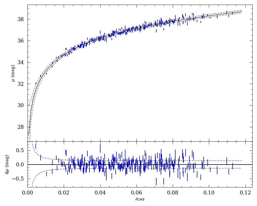
Figure 14: The top panel shows the Hubble diagram of the SNPY_EBV sample with residuals plotted below. The value of $H_{0}$ is degenerate with the absolute magnitude of SNe Ia, amounting to a constant vertical offset. The solid black line shows the $\Lambda$CDM model that zeros the inverse-variance weighted residuals. The dashed lines show the combined uncertainty due to peculiar velocity and intrinsic dispersion.

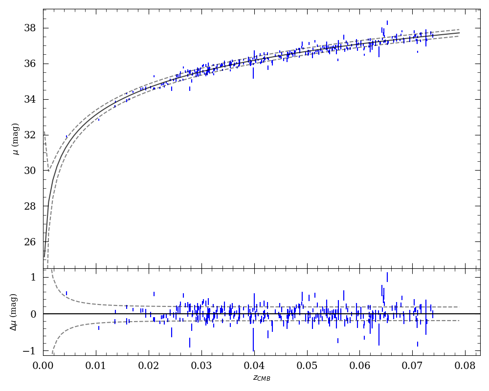
Figure 15: The same as Figure 14, but using the SNPY_Max sample. The limited redshift range is due to the cut requiring the observed filters to map to the CSP $V$ and $r$ filters in the rest frame.

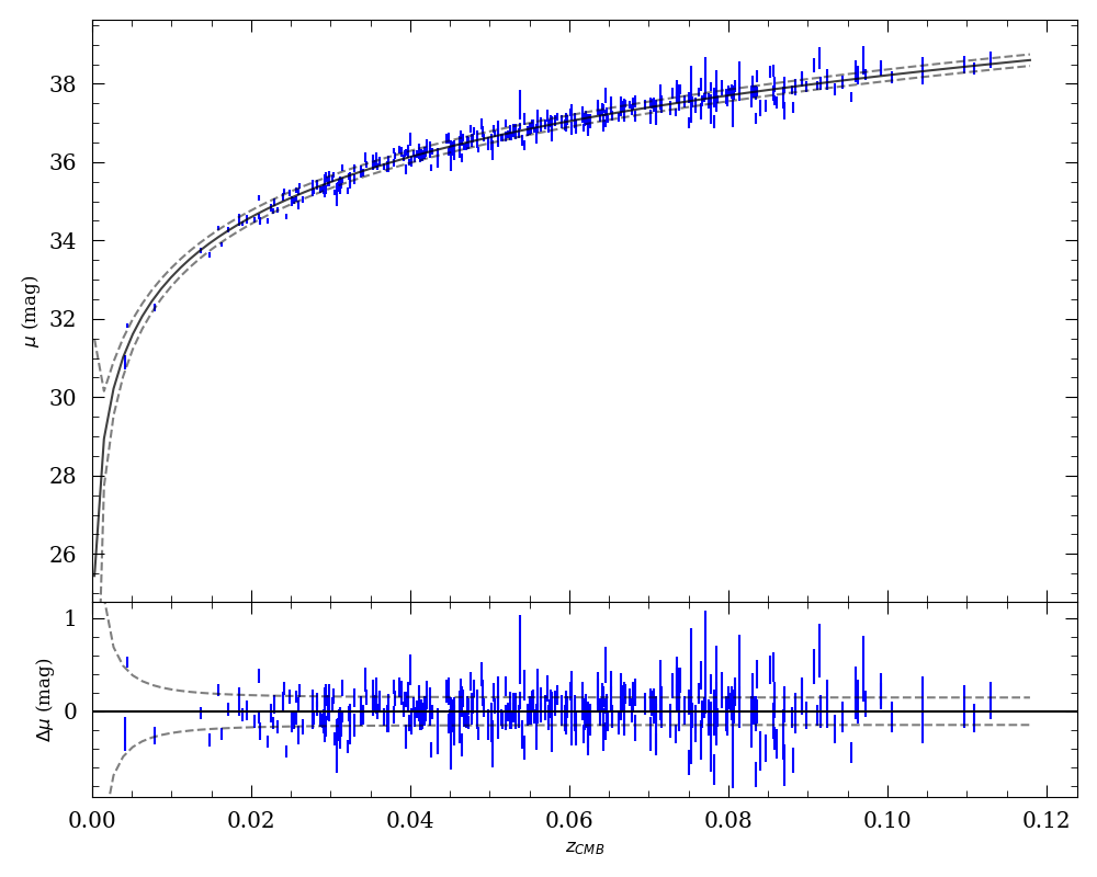
Figure 16: The same as Figure 14, but using the SALT sample.

6.2 Trend with Redshift

There is a trend between the Hubble residuals and redshift in the SNPY_EBV and SALT samples. We perform linear fits using the Bayesian approach detailed in Jaynes & Crow (1999), using flat priors in $\sin(\text{slope})$ and intercept, and a Jeffreys prior on scatter (Jeffreys, 1946).

$$\Delta\mu_{SNPY\_EBV}= -0.6(4)z_{\text{CMB}}\text{ mag}+0.03(02)\text{ mag}$$ (14)

$$\Delta\mu_{SNPY\_Max}= -0.0(5)z_{\text{CMB}}\text{ mag}+0.00(03)\text{ mag}$$ (15)

$$\Delta\mu_{SALT}= 0.3(4)z_{\text{CMB}}\text{ mag}-0.01(02)\text{ mag}$$ (16)

The Hubble residuals in the SNPY_Max sample do not appear to trend with redshift. The differing signs in the slopes of the SNPY_EBV and SALT samples indicate that the issue is due to differences in the fitters rather than a real trend in the data or an issue in the estimation of $\mu_{\text{cos}}$. A review of the SNooPy and SNCosmo code revealed no issue with the programmatic implementation of the methods in the literature (Burns et al., 2011, 2014; Guy et al., 2005, 2007; Kenworthy et al., 2021; Pierel et al., 2022).

The difference between SNPY_EBV and SALT Hubble residuals is seen most clearly in Figure 17. Comparing residuals accounts for the zero-point offset in inferred $\mu$ in each sample and suppresses astrophysical properties that should affect both inferences equally, such as peculiar velocity or intrinsic variation in luminosity. We calculate uncertainties for the differences using the Pearson correlation between the distance modulus uncertainties in each sample.

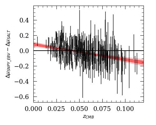
Figure 17: The difference between Hubble residuals from the SNPY_EBV sample ($\Delta_{SNPY\_EBV}$) and the SALT sample ($\Delta_{SALT}$) is anti-correlated with redshift. We fit a linear trend to the data, finding a slope of -2.0(3) mag. The 1- and 2-$\sigma$ contours are in red and light-red.

We tested the SNooPy EBV_model2 and SALT3-NIR by fitting the $r$- and $i$-band photometry of a SN Ia at $z_{\text{CMB}}\approx 0.72$ using both programs. Using the $H_{0}$ and $M$ values from the SNPY_EBV and SALT samples, we found the corresponding fitters produced residual distance moduli of $0.095\pm 0.167$ and $-0.315\pm 0.167$. This indicates that any trend between residual distance modulus and redshift does not continue at higher redshifts.

The trend with redshift could be the result of differences in how the fitters account for shape or colour, which could both evolve with redshift due to selection effects. We investigated whether the SNPY_EBV residuals, SALT residuals, or their differences were correlated with the fitting parameters $s_{BV}$, $E(B-V)_{\text{host}}$, $x_{1}$, and $c$, plotting the results in Figure 18. Correlations imply the fitter is not properly accounting for the effect shape or colour has on the luminosity. In SALT this would mean the standardization parameters $\alpha$ or $\beta$ are improperly calibrated. In SNooPy’s EBV_model2 a correlation between the Hubble residuals and $s_{BV}$ would imply there is a systematic difference between the light curves in our sample and the light curves used for interpolation. A correlation with $E(B-V)_{\text{host}}$ would imply that the reddening law assumed in the EBV_model2 does not fully capture the dust properties affecting our observations.

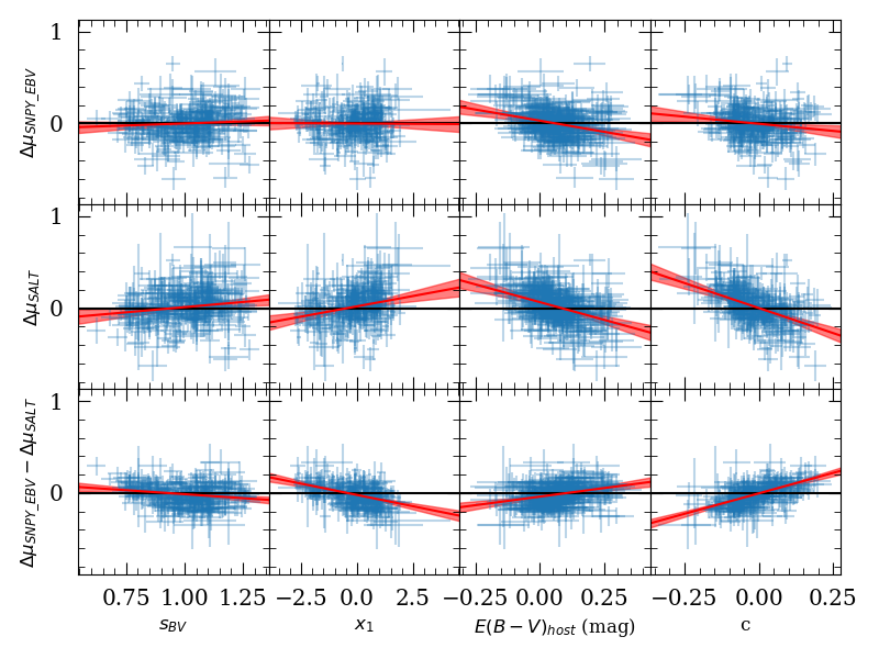
Figure 18: We compare the Hubble residuals in the SNPY_EBV sample, the residuals in the SALT sample, and their differences to the SNooPy fitting parameters $s_{BV}$ and $E(B-V)_{\text{host}}$ and SALT fitting parameters $x_{1}$ and $c$. The best-fitting linear relation is plotted in red with a 95% confidence interval in light red. The strong correlation with colour parameters implies the standardization coefficient $\beta$ is not calibrated correctly for our sample, and that the reddening law assumed in the EBV_model2 may be inappropriate for our sample.

The residuals appear correlated with the colour parameters $E(B-V)_{\text{host}}$ and $c$, with the correlation most obvious in the SALT residuals and the residual differences. This calls our $\beta$ coefficient into question, which comes from an analysis of the SALT sample performed in UNITY. The coefficients are not inferred by minimizing dispersion in the Hubble residuals, but by maximizing a likelihood in a Bayesian hierarchical model. UNITY models the ‘true’ $x_{1}$ and $c$ parameters of a SN Ia as latent variables to account for Eddington bias. The standardization coefficients operate on these ‘true’ values rather than the ‘observed’ values that come from a light curve fit. We compare the ‘true’ and ‘observed’ $x_{1}$ and $c$ parameters in Figure 19. Deviations from one-to-one correspondence come from both statistical error and Eddington bias, which manifests as ‘observed’ parameters scattering away from 0.

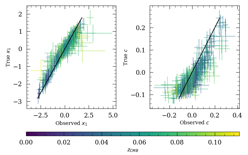
Figure 19: UNITY models the ‘true’ values of $x_{1}$ and $c$ as latent variables in its hierarchical model. We compare these against the ‘observed’ values that come from SALT3-NIR fits, with one-to-one correspondence lines plotted in black. The standardization coefficients from UNITY are calibrated against the true values, and will not minimize Hubble residuals when used with the observed values.

Figure 20 shows that the bias seems more prevalent at higher redshifts. Parameter differences in bins at higher redshifts generally have larger standard deviations, with sample incompleteness heavily affecting bins beyond $z\sim 0.09$. This could indicate that the uncertainties in $x_{1}$ or $c$ are underestimated in fits to noisier data, but verifying such a claim would require simulations beyond the scope of this paper (such as those in Peterson et al. 2024, in prep). Additionally, the median differences in $c$ appear non-zero, especially in lower redshift bins. We have not identified a definitive cause for this behaviour, but speculate that our choice of hyperparameters in UNITY does not allow for the flexibility needed to model the distribution of $c$ over the parameter space spanned by our sample. This could produce a correlation between SALT Hubble residuals and redshift or $c$ independent of $\beta$.

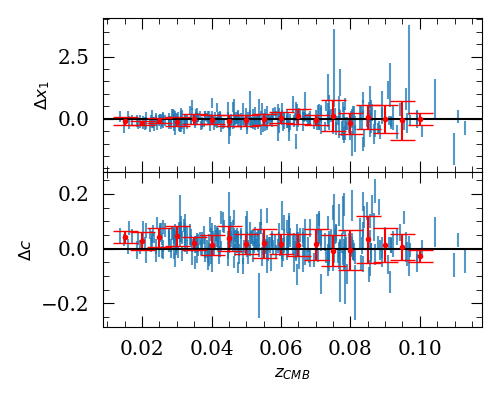
Figure 20: We parametrize the difference between the ‘true’ and ‘observed’ $x_{1}$ and $c$ parameters as $\Delta x_{1}$ and $\Delta c$. The errors in each difference are estimated using the sample Pearson correlation coefficient. The red markers and errorbars show the medians and standard deviations of differences in bins 0.005 wide in redshift space. The standard deviations generally increase with redshift until $z\sim 0.09$, where data is relatively sparse. $\Delta c$ appears offset from 0, especially at lower redshifts. This could imply that the hyperparameters UNITY uses to describe the distribution of $c$ may require more flexibility to accurately model our observations.

To ascertain the validity of using a single $\beta$ value over the entire redshift range, we analysed subsets of the SALT sample in UNITY. We examined subsets consisting of targets within redshift bins of width 0.01, as well as a cumulative sum including all targets below a series of redshifts. Figure 21 shows that the inferred $\beta$ decreases in higher redshift bins, but that it remains relatively stable in the cumulative case. This suggests the hyperparameters describing the distribution of $c$ are robust against higher redshift SNe Ia, but that these SNe prefer a lower value for $\beta$. This assumes the $c$ parameter follows a single distribution over the whole sample, rendering measurements that may suggest otherwise an effect of bias. UNITY permits alternative parametrizations, such as a broken-linear form for $\beta$, but adding such complexity is beyond the scope of this paper. Similarly, more sophisticated analyses of dust properties using SNooPy have been performed with its color_model (e.g. Burns et al., 2018; Johansson et al., 2021) or by using more of the colour information in the max_model (e.g. Uddin et al., 2020, 2023). Implementing and evaluating these approaches will be necessary before using our data for robust cosmological analyses.

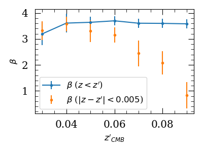
Figure 21: We analyse subsets of the SALT sample using UNITY and show the inferred $\beta$ values as a function of redshift cut value $z^{\prime}_{CMB}$. The blue data show the results from subsets defined by a maximum redshift $z<z^{\prime}$. $\beta$ is relatively stable as the sample expands to include higher redshift targets. The orange data are from redshift bins centred on $z^{\prime}$ and 0.01 wide, such that $|z-z^{\prime}|<0.005$. SNe in higher redshift bins prefer lower $\beta$ values, which could be a result of Eddington bias becoming more significant at greater distances.

Thus, we do not find a satisfactory solution to eliminate the correlations between Hubble residuals and redshift or colour parameter. Empirical corrections are possible using Equations 14, but such an approach is neither physically motivated nor statistically rigorous. More detailed analyses are required to fully understand and rectify this issue.

6.3 The Effect of NIR Photometry on Distance Measurements

As mentioned in section 1.2.1, NIR photometry offers two key benefits when analyzing SNe Ia. The effects of dust are suppressed and SNe Ia demonstrate less variable peak luminosities in the NIR. We examine the benefits of NIR photometry by comparing fits using NIR and optical photometry to fits using only optical photometry. We split our three samples into six: SNPY_EBV_OJ, SNPY_Max_OJ, and SALT_OJ (the OJ samples), which include optical and $J$-band photometry and SNPY_EBV_O, SNPY_Max_O and SALT_O (the O samples), which are their optical-only counterparts. Unlike the SNPY_EBV, SNPY_Max, and SALT samples, which vary in size, target selection, and even bandpasses used to fit a given target, we enforce parity between the OJ and O samples. To do this we prepare the O samples following the same methodology used to produce SNPY_EBV, SNPY_Max, and SALT except without $J$-band photometry. The number of SNe discarded at each cut and the size of the final samples are listed in Table 9. The six samples are made of the SNe common to both the O and OJ samples.

We modify the outlier detection method described in 5.3.1 to highlight disagreement between the OJ and O samples rather than between SNPY_EBV, SNPY_Max, and SALT. This precludes the need to transform SNooPy fitting parameters into SALT parameters. The fitting parameters of SNe in the OJ and O samples produce difference vectors: $m=(\delta t_{0},\delta s_{BV},\delta E(B-V)_{\text{host}})$ for differences between SNPY_EBV_OJ and SNPY_EBV_O, $m=(\delta t_{0},\delta s_{BV},\delta(V-r))$ for differences between SNPY_Max_OJ and SNPY_Max_O, and $m=(\delta t_{0},\delta m^{*}_{B},\delta x_{1},\delta c)$ for differences between SALT_OJ and SALT_O. We use the Mahalanobis distance $d(m,D)=\sqrt{m\Sigma^{-1}m^{T}}$ to identify outliers, once again approximating the covariance matrix $\Sigma$ by bootstrap resampling the parameter differences 5,000 times and averaging the sample covariances. The distributions of Mahalanobis distances for samples the three pairs of samples are given in Figure 22.

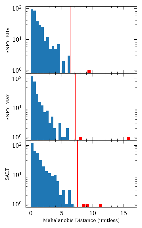
Figure 22: Our first outlier detection algorithm is based on agreement between models fit with and without $J$-band photometry as quantified by the Mahalanobis distance between parameter differences and the origin, representing a SN with identical estimates in the OJ and O samples. A greater distance indicates greater disagreement between fits, with significant disagreement indicating at least one of the models is unreliable.

Cuts	SNPY_EBV_O Cut	Remaining	SNPY_Max_O Cut	Remaining	SALT_O Cut	Remaining
Passed Sample Wide Cuts		441		441		441
Successful Fit	1	440	1	440	0	441
Rest frame $m_{V}$ and $m_{r}$			83	362
$0.6<s_{BV}<1.3$	27	413	35	327
$\sigma_{s_{BV}}<0.2$	3	410	5	322
$E(B-V)_{\mathrm{host}}<0.3$ mag	54	356
$|x_{1}|<3$					17	424
$\sigma_{x_{1}}<1.5$					0	424
$|c|<0.3$					35	389
$\sigma_{c}<0.2$					5	384
Phase Requirements	1	355	2	320	2	382
Reduced $\chi^{2}<6.66$	10	345	16	304	14	368
Also In $OJ$ Sample	27	318	14	290	21	347
$d_{M}<5\sigma_{d_{M}}$	1	317	2	288	1	346
UNITY Outlier	6	311	8	280	8	338

Table 9: Similar to Table 6, we list the number of SNe discarded at each cut for our optical-only samples. We begin after the survey wide cuts of Table 5, starting with the number of successful fits in SNooPy’s EBV_model2 (SNPY_EBV_O), max_model (SNPY_Max_O), and SALT3-NIR (SALT_O). Our final two cuts are based on outlier detection.

Sample	RMS (mag)	WRMS (mag)	NMAD (mag)	$\sigma_{int}$ (mag)
SNPY_EBV_OJ	$0.169(009)$	$0.158(008)$	$0.150(010)$	$0.126(011)$
SNPY_EBV_O	$0.174(009)$	$0.168(010)$	$0.161(011)$	$0.135(012)$
SNPY_Max_OJ	$0.227(017)$	$0.190(013)$	$0.169(013)$	$0.189(015)$
SNPY_Max_O	$0.297(025)$	$0.239(016)$	$0.196(014)$	$0.275(025)$
SALT_OJ	$0.202(009)$	$0.186(010)$	$0.175(012)$	$0.147(010)$
SALT_O	$0.198(010)$	$0.193(011)$	$0.175(013)$	$0.141(012)$

Table 10: Adding NIR photometry does not lead to statistically significant decreases in the various measures of dispersion. Each estimator is calculated after bootstrap resampling the Hubble residuals 5,000 times. The value is the average and the uncertainty is the standard deviation.

Measurements of dispersion in each sample’s Hubble residuals are presented in Table 10. We characterize the differences between the OJ and O samples in the method we used when varying photometry in Section 4.1.2. The various estimators show a general decrease in dispersion when adding $J$-band photometry to the O samples, but none of the differences is inconsistent with 0. Histograms of the resampled dispersion differences are plotted in Figure 23. The distributions of differences may have non-zero centres, but are all consistent with 0, meaning the trend of lower dispersions in the OJ samples is not statistically significant. This does not imply other methodologies do not or cannot benefit from the $J$-band photometry, but that with our samples, cuts, and methods, we cannot definitively say NIR photometry leads to smaller Hubble residuals.

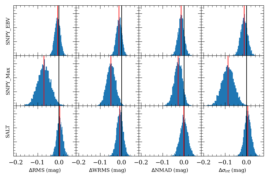
Figure 23: We recorded various measures of dispersion over 5,000 iterations of bootstrap resampling, and show the distribution of differences between the OJ and O samples. Including $J$-band photometry with the optical data typically leads to decreases in the three tested measures of dispersion in Hubble residuals and the inferred intrinsic dispersion, but those differences are usually within one standard deviation of 0 mag for the SNPY_EBV and SALT samples. The SNPY_Max sample varies more, indicating that a Tripp calibration based on $J$-band peak magnitudes may be more precise than one based on the $V$-band.

7 Discussion

The RMS of the Hubble residuals is 0.174 mag in the SNPY_EBV sample ($N=338$), 0.213 mag in the SNPY_Max sample ($N=294$), and 0.203 mag in the SALT sample ($N=354$). Our result goes against a number of studies which support the use of NIR photometry in deriving distances to SNe Ia, but is not alone in finding relatively large dispersions. Stanishev et al. (2018) combine optical and NIR light curves from numerous sources, including new observations, and find RMS values of $\sim$0.15 mag ($N\sim 120$) while Johansson et al. (2021) did the same and found an RMS of 0.19 mag ($N=165$). Notably, the sub-sample of 16 new SNe Ia presented in Stanishev et al. (2018) were only imaged once or twice in the NIR, and the RMS of their residuals is $\sim$0.2. Sparsity may play a role in the greater dispersion, but Müller-Bravo et al. (2022) found that the effect is relatively small, bringing an RMS of 0.166 mag to 0.180 mag ($N=36$) when removing all but one epoch from $J$-band light-curves.

One key difference between our work and those which find smaller dispersions is that our analysis does not force SNe Ia to be standard candles in the NIR. It may be possible that variation in SN Ia NIR luminosity, if it does vary, is not parametrized by the correlations observed in the optical. In our comparison with Peterson et al. (2023) we found that our fitting methods applied to their $YJH$ data resulted in large dispersion, whereas they fixed the shape and color parameters in the NIR-only fits to be 0, removing any variation in luminosity between SNe, and measured lower dispersion than when using bandpass combinations including optical data from ATLAS. This is similar to Avelino et al. (2019), who treated SNe Ia as standard candles in the NIR and found that smaller Hubble residuals than those from optical-only fits using SNooPy or SALT2. That said, not all studies favour this approach. Jones et al. (2022) measured Hubble residual scatter over several analyses of 79 SNe Ia and measured a RMS of $\sim$0.17 mag using SNooPy to fit only NIR data, and $\sim$0.14 mag when including optical data with $R_{V}=1.52$. The optical and NIR RMS increased to $\sim$0.18 mag when using a Milky Way-like value of $R_{V}=3.1$, emphasizing the importance of assumptions regarding dust. Similarly, Pierel et al. (2022) examined the performance of SALT3-NIR, SALT3, and SNooPy over various bandpass combinations and model parametrizations. They found a Hubble residual RMS of $\sim$0.12 mag ($N=24$) when using SALT3-NIR with optical and $YJH$ data, fitting for shape and colour, and a greater RMS of $\sim$0.13 mag for the same sample using only $YJH$ data and keeping the shape and colour parameters fixed at 0.

As explored in Section 6.2, there is a trend between redshift and the Hubble residuals in SNPY_EBV and SALT. Correcting this trend empirically will decrease the dispersion of the Hubble residuals, but such an a posteriori treatment invites bias. There are several other obvious ways to decrease the measured dispersion. One could calibrate $\alpha$ or $\beta$ by minimizing Hubble residuals, employ corrections by the redshift bin, or use cuts based on Hubble residuals such as Chauvanet’s crietrion or $\sigma$-clipping. There is ample motivation for using such techniques. Our robust measure of dispersion, NMAD, is consistently lower than RMS and WRMS in all three samples, which suggests that there are SNe Ia in our samples could be considered outliers. However, we choose to present our results as we found them to avoid contaminating them with ad hoc corrections.

The study of SNe Ia in the NIR has advanced as more data have become available, but there are still challenges that must be met to maximize the potential benefits. At the moment it is unclear whether SNe Ia are standard candles in the NIR or simply require less standardization than in the optical. Similarly, it is not clear if the shape-luminosity correlation observed in the optical is still the primary mode of variation in the NIR. Answering these questions will require various kinds of data. Spectral time series provide unique views into the physical mechanisms of SNe Ia, while also improving the accuracy of K-corrections. High-cadence, multi-band observations like those pursued by the DEHVILS survey are vital for building standardization models. The Hawai‘i Supernova Flows project provides a valuable test bed for SN Ia research through its unprecedented sample size.

8 Conclusion

This paper introduces the Hawai‘i Supernova Flows project, a peculiar velocity survey designed to obtain systematics-limited distances to SNe Ia while consuming minimal dedicated observational resources. We review the observational components of our project: optical photometry from public all-sky surveys, NIR photometry from UKIRT, and optical spectroscopy from the UH 2.2 m and Subaru. We validate our methods and data against external sources. We use SDSS spectra to find that our redshift inferences are typically within 45 km s^-1 of the values in HyperLEDA. The absolute wavelength calibration of our spectroscopic observations introduces minimal error, producing redshifts typically within 48 km s^-1 of their published values. Using our methodology to fit data from our partner program DEHVILS, we found no increase in the dispersion of Hubble residuals when using only optical data, or using optical and NIR data with SNooPy’s EBV_model2. The increase in dispersion seen when using SALT3-NIR seems to come from our choice to calibrate the standardization coefficients with UNITY instead of only using the Hubble residuals. Our independent photometric reductions of the same $J$-band observations are consistent, producing similar dispersions. Given cuts on both SNooPy and SALT fitting parameters, our three final samples include 338, 294, and 354 SNe. The RMS values of their Hubble residuals are 0.174, 0.213, and 0.203 mag.

The Nancy Grace Roman space telescope will obtain rest-frame NIR observations of SNe Ia within $z\sim 0.7$ (Hounsell et al., 2018; Rose et al., 2021), necessitating the maturation of SN Ia cosmology in the NIR. Thus far, the majority of publicly available NIR SN Ia light-curves have come from CSP-I (N=123 Krisciunas et al., 2017), CfAIR2 (N=94 Friedman et al., 2015), or recent work from our partner program DEHVILS (N=96 Peterson et al., 2023). Data from CSP-II (N=214 Phillips et al., 2019; Hsiao et al., 2019), the SIRAH program (N=24, HST-GO 15889; Jha et al., 2019), and other exciting projects are expected in the near future. Upon publication of this work, we will release NIR observations of 1218 transients, including 669 spectroscopically classified SNe Ia, 397 of which are in at least one of our final samples, and 192 spectroscopic redshifts for SN Ia host-galaxies that have not been previously measured. The NIR photometry of the Hawai‘i Supernova Flows project is the largest homogeneous collection of its kind in terms of unique SNe Ia. This growing sample will provide increasing resolution into peculiar velocities as a function of position on the sky and redshift, permitting us to map the structure of dark matter.

9 Data Availability

Upon publication, we will release the following data via https://www.github.com/ado8/hsf_DR1:

• $J$-band light-curves of all observed targets regardless of spectroscopic classification

• Weighted cross-correlation results for all galaxies we observed with SNIFS or FOCAS

• Multiple sets of fitting parameters and uncertainties for all spectroscopically confirmed SNe Ia, with sets covering all combinations of fitting model (EBV_model2, max_model, SALT3-NIR) and data used (optical only or optical and NIR)

• Additional sets of fitting parameters for SNe Ia used in our comparisons with DEHVILS and CSP

The code used in our analysis will be available via https://www.github.com/ado8/hsf_code. Data such as images and spectra may be available upon reasonable request.

10 Acknowledgements

This work, AD, and BS are supported by National Science Foundation grant AST-1911074.

AD and KSM are supported by the European Research Council (ERC) under the European Union’s Horizon 2020 research and innovation programme (Grant Agreement No. 101002652).

This publication makes use of data products from the Two Micron All Sky Survey, which is a joint project of the University of Massachusetts and the Infrared Processing and Analysis Center/California Institute of Technology, funded by the National Aeronautics and Space Administration and the National Science Foundation.

The Pan-STARR Surveys (PS1) and the PS1 public science archive have been made possible through contributions by the Institute for Astronomy, the University of Hawaii, the Pan-STARRS Project Office, the Max-Planck Society and its participating institutes, the Max Planck Institute for Astronomy, Heidelberg and the Max Planck Institute for Extraterrestrial Physics, Garching, The Johns Hopkins University, Durham University, the University of Edinburgh, the Queen’s University Belfast, the Harvard-Smithsonian Center for Astrophysics, the Las Cumbres Observatory Global Telescope Network Incorporated, the National Central University of Taiwan, the Space Telescope Science Institute, the National Aeronautics and Space Administration under Grant No. NNX08AR22G issued through the Planetary Science Division of the NASA Science Mission Directorate, the National Science Foundation Grant No. AST-1238877, the University of Maryland, Eotvos Lorand University (ELTE), the Los Alamos National Laboratory, and the Gordon and Betty Moore Foundation.

This research has made use of NASA’s Astrophysics Data System.

We acknowledge the usage of the HyperLeda database (http://leda.univ-lyon1.fr).

This research has made use of the SIMBAD database, operated at CDS, Strasbourg, France

This research has made use of the NASA/IPAC Extragalactic Database (NED), which is funded by the National Aeronautics and Space Administration and operated by the California Institute of Technology.

UKIRT is owned by the University of Hawaii (UH) and operated by the UH Institute for Astronomy. When (some of) the data reported here were obtained, the operations were enabled through the cooperation of the East Asian Observatory.

The ZTF forced-photometry service was funded under the Heising-Simons Foundation grant #12540303 (PI: Graham).

This work has made use of data from the European Space Agency (ESA) mission Gaia (https://www.cosmos.esa.int/gaia), processed by the Gaia Data Processing and Analysis Consortium (DPAC, https://www.cosmos.esa.int/web/gaia/dpac/consortium). Funding for the DPAC has been provided by national institutions, in particular the institutions participating in the Gaia Multilateral Agreement.

We acknowledge ESA Gaia, DPAC and the Photometric Science Alerts Team (http://gsaweb.ast.cam.ac.uk/alerts).

Funding for the Sloan Digital Sky Survey (SDSS) has been provided by the Alfred P. Sloan Foundation, the Participating Institutions, the National Aeronautics and Space Administration, the National Science Foundation, the U.S. Department of Energy, the Japanese Monbukagakusho, and the Max Planck Society. The SDSS Web site is http://www.sdss.org/.

The SDSS is managed by the Astrophysical Research Consortium (ARC) for the Participating Institutions. The Participating Institutions are The University of Chicago, Fermilab, the Institute for Advanced Study, the Japan Participation Group, The Johns Hopkins University, the Korean Scientist Group, Los Alamos National Laboratory, the Max-Planck-Institute for Astronomy (MPIA), the Max-Planck-Institute for Astrophysics (MPA), New Mexico State University, University of Pittsburgh, University of Portsmouth, Princeton University, the United States Naval Observatory, and the University of Washington.

Appendix A NIR Photometry and Late-time Observations

When late-time observations are available, our forward-modelling photometry process produces measurements consistent with those from template-subtracted images. The importance of the late-time observation seems to vary based on the location of the SN relative to its host galaxy. Nuclear transients and SNe coincident with sharp features are critically dependent on late-time observations, whereas photometric measurements of other SNe do not change significantly with or without late-time observations. This motivates the use of a mixture model to simultaneously model those two populations. For each SN, we create two ensembles of images; one with and one without late-time observations. This provides two values for the magnitude of the SN at each observed epoch, $m_{ref}$ and $m_{0}$ respectively. The differences $\Delta m=m_{ref}-m_{0}$ should be distributed about 0 mag if $m_{ref}$ and $m_{0}$ are normally distributed about the same mean. We use Stan to infer the population means, standard deviations, and the mixing ratio.

Our priors are based on a crude analysis where we consider the subset $|\Delta m|\leq 0.5$ mag and $|\Delta m|>0.5$ mag, where 0.5 was chosen arbitrarily. The subset near 0 comprises 299 of our 328 observations. Our prior on the mixing ratio is a Beta distribution with $\alpha$ = 3 and $\beta$ = 0.3 such that the mean expectation value $\frac{\alpha}{\alpha+\beta}\approx 299/328$. The scale of $\alpha$ and $\beta$ was chosen to create a moderately informed prior. Our priors on the population means are $\mu_{0}\sim\mathcal{N}(0,0.1)$ for the tightly dispersed population, and $\mu_{1}\sim\mathcal{U}(-\infty,\infty)$ for the late-time sensitive population. Lastly, our priors on the standard deviations are $\sigma\sim\mathcal{N}(0,2)$, with $0<\sigma_{0}<\sigma_{1}$.

We fit a Gaussian mixture-model to the photometric differences using Stan (Carpenter et al., 2017) and find 83.3% of the differences appear tightly dispersed ($\Delta m\sim\mathcal{N}(0.02\pm 0.006\mathrm{mag},0.08\pm 0.007\mathrm{mag})$), and the remaining 16.7% vary much more dramatically ($\Delta m\sim\mathcal{N}(0.37\pm 0.131\mathrm{mag},0.94\pm 0.110\mathrm{mag})$). The fraction of targets reliant upon late-time observations for accurate photometry is vastly exaggerated in this analysis because the subsample comprises only targets manually determined to need late-time observations. The critical information is the distribution of the tightly dispersed population, which describes the effect late-time observations have on typical photometric measurements.

Appendix B Host Galaxy Identification Algorithm

Before choosing to proceed with manual host galaxy identification, we investigated the Directional Light Radius method (DLR; Sullivan et al., 2006; Sako et al., 2018) which normalizes angular separation by the elliptical radius of a galaxy in the direction of the transient. The morphological data came from the NASA/IPAC Extragalactic Database (NED; Helou et al., 1991; Mazzarella & NED Team, 2007), the Simbad Astronomical Database (Simbad; Wenger et al., 2000), and the GLADE+ Galaxy Catalog (GLADE+; Dálya et al., 2022), which itself consolidates galaxies from the Gravitational Wave Galaxy Catalogue (White et al., 2011), HyperLEDA (Makarov et al., 2014), and the 2MASS Extended Source Catalog (Jarrett et al., 2000; Skrutskie et al., 2006). Unfortunately, the heterogeneity and sparsity of the available data presented several failure modes. Firstly, the correct host galaxy could not be identified if it was not included in at least one of the aforementioned databases or catalogues. Similarly, if a galaxy’s morphological data was not available, the DLR method could not be applied. Lastly, if multiple galaxies have categorically distinct morphological measurements, either using different filters or different metrics, the DLR method would have been biased.

References

- Adelman-McCarthy et al. (2007) Adelman-McCarthy J. K., et al., 2007, ApJS, 172, 634
- Aggarwal et al. (2021) Aggarwal K., Budavári T., Deller A. T., Eftekhari T., James C. W., Prochaska J. X., Tendulkar S. P., 2021, ApJ, 911, 95
- Alard & Lupton (1998) Alard C., Lupton R. H., 1998, ApJ, 503, 325
- Alard & Lupton (1999) Alard C., Lupton R., 1999, ISIS: A method for optimal image subtraction, Astrophysics Source Code Library, record ascl:9909.003 (ascl:9909.003)
- Amanullah et al. (2010) Amanullah R., et al., 2010, ApJ, 716, 712
- Anand et al. (2021) Anand G. S., et al., 2021, AJ, 162, 80
- Ashall et al. (2016) Ashall C., Mazzali P., Sasdelli M., Prentice S. J., 2016, Monthly Notices of the Royal Astronomical Society, 460, 3529
- Ashall et al. (2021) Ashall C., et al., 2021, The Astrophysical Journal, 922, 205
- Avelino et al. (2019) Avelino A., Friedman A. S., Mandel K. S., Jones D. O., Challis P. J., Kirshner R. P., 2019, ApJ, 887, 106
- Barbary et al. (2022) Barbary K., et al., 2022, SNCosmo, doi:10.5281/zenodo.7117347, https://doi.org/10.5281/zenodo.7117347
- Barone-Nugent et al. (2012) Barone-Nugent R. L., et al., 2012, MNRAS, 425, 1007
- Bellm et al. (2019) Bellm E. C., et al., 2019, PASP, 131, 018002
- Bertone & Hooper (2018) Bertone G., Hooper D., 2018, Reviews of Modern Physics, 90, 045002
- Bertschinger & Dekel (1989) Bertschinger E., Dekel A., 1989, ApJ, 336, L5
- Blondin et al. (2011) Blondin S., Mandel K. S., Kirshner R. P., 2011, A&A, 526, A81
- Boone et al. (2021) Boone K., et al., 2021, The Astrophysical Journal, 912, 71
- Brout & Scolnic (2020) Brout D., Scolnic D. M., 2020, The Astrophysical Journal, 909
- Brout & Scolnic (2021) Brout D., Scolnic D., 2021, ApJ, 909, 26
- Brout et al. (2022) Brout D., et al., 2022, ApJ, 938, 110
- Burns et al. (2011) Burns C. R., et al., 2011, AJ, 141, 19
- Burns et al. (2014) Burns C. R., et al., 2014, ApJ, 789, 32
- Burns et al. (2018) Burns C. R., et al., 2018, ApJ, 869, 56
- Campbell et al. (2014) Campbell L. A., et al., 2014, Monthly Notices of the Royal Astronomical Society, 443, 1231
- Cardelli et al. (1989) Cardelli J. A., Clayton G. C., Mathis J. S., 1989, ApJ, 345, 245
- Carpenter et al. (2017) Carpenter B., et al., 2017, Journal of Statistical Software, 76, 1–32
- Carrick et al. (2015) Carrick J., Turnbull S. J., Lavaux G., Hudson M. J., 2015, Monthly Notices of the Royal Astronomical Society, 450, 317
- Casali, M. et al. (2007) Casali, M. et al., 2007, A&A, 467, 777
- Chambers et al. (2016) Chambers K. C., et al., 2016, arXiv e-prints, p. arXiv:1612.05560
- Chang et al. (2015) Chang Y.-Y., van der Wel A., da Cunha E., Rix H.-W., 2015, ApJS, 219, 8
- Collaboration et al. (2022) Collaboration D., et al., 2022, The Astronomical Journal, 164, 207
- Conley et al. (2008) Conley A., et al., 2008, ApJ, 681, 482
- Contreras et al. (2010) Contreras C., et al., 2010, AJ, 139, 519
- Courtois et al. (2012) Courtois H. M., Hoffman Y., Tully R. B., Gottlöber S., 2012, ApJ, 744, 43
- Courtois et al. (2017) Courtois H. M., Tully R. B., Hoffman Y., Pomarède D., Graziani R., Dupuy A., 2017, ApJ, 847, L6
- Dálya et al. (2022) Dálya G., et al., 2022, MNRAS, 514, 1403
- Davis & Scrimgeour (2014) Davis T. M., Scrimgeour M. I., 2014, MNRAS, 442, 1117
- Dekel et al. (1990) Dekel A., Bertschinger E., Faber S. M., 1990, ApJ, 364, 349
- Dekel et al. (1999) Dekel A., Eldar A., Kolatt T., Yahil A., Willick J. A., Faber S. M., Courteau S., Burstein D., 1999, ApJ, 522, 1
- Desai et al. (2024) Desai D. D., et al., 2024, Monthly Notices of the Royal Astronomical Society, p. stae606
- Dhawan et al. (2018) Dhawan S., Jha S. W., Leibundgut B., 2018, A&A, 609, A72
- Djorgovski & Davis (1987) Djorgovski S., Davis M., 1987, ApJ, 313, 59
- Draine (2003) Draine B. T., 2003, ApJ, 598, 1017
- Dressler et al. (1987) Dressler A., Lynden-Bell D., Burstein D., Davies R. L., Faber S. M., Terlevich R., Wegner G., 1987, ApJ, 313, 42
- Dye et al. (2018) Dye S., et al., 2018, MNRAS, 473, 5113
- Eastmond & Abell (1978) Eastmond T. S., Abell G. O., 1978, PASP, 90, 367
- Ebizuka et al. (2011) Ebizuka N., et al., 2011, Publications of the Astronomical Society of Japan, 63, S613
- Feldman & Watkins (2008) Feldman H. A., Watkins R., 2008, Monthly Notices of the Royal Astronomical Society, 387, 825
- Feldman et al. (2010) Feldman H. A., Watkins R., Hudson M. J., 2010, Monthly Notices of the Royal Astronomical Society, 407, 2328
- Fitzpatrick (1999) Fitzpatrick E. L., 1999, PASP, 111, 63
- Folatelli et al. (2010) Folatelli G., et al., 2010, AJ, 139, 120
- Foley et al. (2017) Foley R. J., et al., 2017, Monthly Notices of the Royal Astronomical Society, 475, 193
- Foreman-Mackey et al. (2013) Foreman-Mackey D., Hogg D. W., Lang D., Goodman J., 2013, PASP, 125, 306
- Förster et al. (2021) Förster F., et al., 2021, AJ, 161, 242
- Freedman et al. (2020) Freedman W. L., et al., 2020, The Astrophysical Journal, 891, 57
- Friedman et al. (2015) Friedman A. S., et al., 2015, ApJS, 220, 9
- Gaia Collaboration et al. (2016) Gaia Collaboration et al., 2016, A&A, 595, A1
- Gaia Collaboration et al. (2018) Gaia Collaboration et al., 2018, A&A, 616, A1
- Galbany et al. (2022) Galbany L., et al., 2022, arXiv e-prints, p. arXiv:2209.02546
- Ganon & Hoffman (1993) Ganon G., Hoffman Y., 1993, ApJ, 415, L5
- Gao et al. (2016) Gao F., et al., 2016, The Astrophysical Journal, 817, 128
- Graham et al. (2019) Graham M. J., et al., 2019, Publications of the Astronomical Society of the Pacific, 131, 078001
- Grayling et al. (2024) Grayling M., Thorp S., Mandel K. S., Dhawan S., Uzsoy A. S., Boyd B. M., Hayesn E. E., Ward S. M., 2024, arXiv e-prints, p. arXiv:2401.08755
- Graziani et al. (2019) Graziani R., Courtois H. M., Lavaux G., Hoffman Y., Tully R. B., Copin Y., Pomarède D., 2019, MNRAS, 488, 5438
- Gupta et al. (2016) Gupta R. R., et al., 2016, The Astronomical Journal, 152, 154
- Guy et al. (2005) Guy J., Astier P., Nobili S., Regnault N., Pain R., 2005, A&A, 443, 781
- Guy et al. (2007) Guy J., et al., 2007, A&A, 466, 11
- Guy et al. (2010) Guy J., et al., 2010, A&A, 523, A7
- Hambly et al. (2008) Hambly N. C., et al., 2008, Monthly Notices of the Royal Astronomical Society, 384, 637
- Hamuy & Pinto (2002) Hamuy M., Pinto P. A., 2002, ApJ, 566, L63
- Hamuy et al. (1995) Hamuy M., Phillips M. M., Maza J., Suntzeff N. B., Schommer R. A., Aviles R., 1995, AJ, 109, 1
- Hamuy et al. (2003) Hamuy M., et al., 2003, Nature, 424, 651
- Hamuy et al. (2006) Hamuy M., et al., 2006, PASP, 118, 2
- Hart et al. (2023) Hart K., et al., 2023, arXiv e-prints, p. arXiv:2304.03791
- Hayden et al. (2021) Hayden B., et al., 2021, ApJ, 912, 87
- Helou et al. (1991) Helou G., Madore B. F., Schmitz M., Bicay M. D., Wu X., Bennett J., 1991, in Albrecht M. A., Egret D., eds, Astrophysics and Space Science Library Vol. 171, Databases and On-line Data in Astronomy. pp 89–106, doi:10.1007/978-94-011-3250-3_10
- Herrnstein et al. (1999) Herrnstein J. R., et al., 1999, Nature, 400, 539
- Hewett et al. (2006) Hewett P. C., Warren S. J., Leggett S. K., Hodgkin S. T., 2006, Monthly Notices of the Royal Astronomical Society, 367, 454
- Hicken et al. (2007) Hicken M., Garnavich P. M., Prieto J. L., Blondin S., DePoy D. L., Kirshner R. P., Parrent J., 2007, The Astrophysical Journal, 669, L17
- Hodapp et al. (2004) Hodapp K. W., et al., 2004, in Amico P., Beletic J. W., Beletic J. E., eds, Scientific Detectors for Astronomy. Springer Netherlands, Dordrecht, pp 501–510
- Hodapp et al. (2018) Hodapp K. W., et al., 2018, in Marshall H. K., Spyromilio J., eds, Vol. 10700, Ground-based and Airborne Telescopes VII. SPIE, p. 107002Z, doi:10.1117/12.2311923, https://doi.org/10.1117/12.2311923
- Hodgkin et al. (2009) Hodgkin S. T., Irwin M. J., Hewett P. C., Warren S. J., 2009, Monthly Notices of the Royal Astronomical Society, 394, 675
- Hoffman et al. (2017) Hoffman Y., Pomarède D., Tully R. B., Courtois H. M., 2017, Nature Astronomy, 1, 0036
- Holoien et al. (2020) Holoien T. W. S., et al., 2020, ApJ, 898, 161
- Holz & Hughes (2005) Holz D. E., Hughes S. A., 2005, The Astrophysical Journal, 629, 15
- Hounsell et al. (2018) Hounsell R., et al., 2018, ApJ, 867, 23
- Howell et al. (2006) Howell D. A., et al., 2006, Nature, 443, 308
- Howlett et al. (2022) Howlett C., Said K., Lucey J. R., Colless M., Qin F., Lai Y., Tully R. B., Davis T. M., 2022, MNRAS, 515, 953
- Hsiao et al. (2007) Hsiao E. Y., Conley A., Howell D. A., Sullivan M., Pritchet C. J., Carlberg R. G., Nugent P. E., Phillips M. M., 2007, ApJ, 663, 1187
- Hsiao et al. (2019) Hsiao E. Y., et al., 2019, PASP, 131, 014002
- Humason et al. (1956) Humason M. L., Mayall N. U., Sandage A. R., 1956, AJ, 61, 97
- Jarrett et al. (2000) Jarrett T. H., Chester T., Cutri R., Schneider S., Skrutskie M., Huchra J. P., 2000, AJ, 119, 2498
- Jaynes & Crow (1999) Jaynes E. T., Crow W. J., 1999. https://api.semanticscholar.org/CorpusID:18814871
- Jeffreys (1946) Jeffreys H., 1946, Proceedings of the Royal Society of London Series A, 186, 453
- Jha et al. (2007) Jha S., Riess A. G., Kirshner R. P., 2007, The Astrophysical Journal, 659, 122
- Jha et al. (2019) Jha S. W., et al., 2019, Supernovae in the Infrared avec Hubble, HST Proposal. Cycle 27, ID. #15889
- Johansson et al. (2021) Johansson J., et al., 2021, ApJ, 923, 237
- Jones et al. (2022) Jones D. O., et al., 2022, The Astrophysical Journal, 933, 172
- Kasen (2006) Kasen D., 2006, ApJ, 649, 939
- Kashikawa et al. (2002) Kashikawa N., et al., 2002, PASJ, 54, 819
- Kashlinsky et al. (2008) Kashlinsky A., Atrio-Barandela F., Kocevski D., Ebeling H., 2008, The Astrophysical Journal, 686, L49
- Kattner et al. (2012) Kattner S., et al., 2012, Publications of the Astronomical Society of the Pacific, 124, 114
- Kelly et al. (2010) Kelly P. L., Hicken M., Burke D. L., Mandel K. S., Kirshner R. P., 2010, ApJ, 715, 743
- Kenworthy et al. (2021) Kenworthy W. D., et al., 2021, The Astrophysical Journal, 923, 265
- Kessler et al. (2009) Kessler R., et al., 2009, PASP, 121, 1028
- Kim et al. (1996) Kim A., Goobar A., Perlmutter S., 1996, PASP, 108, 190
- Kochanek et al. (2017) Kochanek C. S., et al., 2017, PASP, 129, 104502
- Kourkchi et al. (2020) Kourkchi E., et al., 2020, The Astrophysical Journal, 902, 145
- Krisciunas et al. (2017) Krisciunas K., et al., 2017, AJ, 154, 211
- Kunz et al. (2007) Kunz M., Bassett B. A., Hlozek R. A., 2007, Phys. Rev. D, 75, 103508
- Lampeitl et al. (2010) Lampeitl H., et al., 2010, ApJ, 722, 566
- Lantz et al. (2004) Lantz B., et al., 2004, in Mazuray L., Rogers P. J., Wartmann R., eds, Society of Photo-Optical Instrumentation Engineers (SPIE) Conference Series Vol. 5249, Optical Design and Engineering. pp 146–155, doi:10.1117/12.512493
- Lavaux (2016) Lavaux G., 2016, MNRAS, 457, 172
- Lavaux et al. (2010) Lavaux G., Tully R. B., Mohayaee R., Colombi S., 2010, The Astrophysical Journal, 709, 483
- Lawrence et al. (2007) Lawrence A., et al., 2007, MNRAS, 379, 1599
- Leavitt & Pickering (1912) Leavitt H. S., Pickering E. C., 1912, Harvard College Observatory Circular, 173, 1
- Léget et al. (2020) Léget P. F., et al., 2020, A&A, 636, A46
- Li et al. (2003) Li W., et al., 2003, Publications of the Astronomical Society of the Pacific, 115, 453
- Liu et al. (2023) Liu Z.-W., Röpke F. K., Han Z., 2023, Research in Astronomy and Astrophysics, 23, 082001
- Lu et al. (2023) Lu J., et al., 2023, The Astrophysical Journal, 948, 27
- Mahalanobis (1930) Mahalanobis P. C., 1930, Journal and Proceedings of Asiatic Society of Bengal New series, 26, 541
- Makarov et al. (2014) Makarov D., Prugniel P., Terekhova N., Courtois H., Vauglin I., 2014, A&A, 570, A13
- Mandel et al. (2009) Mandel K. S., Wood-Vasey W. M., Friedman A. S., Kirshner R. P., 2009, ApJ, 704, 629
- Mandel et al. (2011) Mandel K. S., Narayan G., Kirshner R. P., 2011, The Astrophysical Journal, 731, 120
- Mandel et al. (2022) Mandel K. S., Thorp S., Narayan G., Friedman A. S., Avelino A., 2022, MNRAS, 510, 3939
- Mazzarella & NED Team (2007) Mazzarella J. M., NED Team 2007, in Shaw R. A., Hill F., Bell D. J., eds, Astronomical Society of the Pacific Conference Series Vol. 376, Astronomical Data Analysis Software and Systems XVI. p. 153
- Möller & de Boissière (2020) Möller A., de Boissière T., 2020, MNRAS, 491, 4277
- Moreno-Raya et al. (2016) Moreno-Raya M. E., Mollá M., López-Sánchez Á. R., Galbany L., Vílchez J. M., Rosell A. C., Domínguez I., 2016, The Astrophysical Journal, 818, L19
- Müller-Bravo et al. (2022) Müller-Bravo T. E., et al., 2022, A&A, 665, A123
- Neill et al. (2009) Neill J. D., et al., 2009, ApJ, 707, 1449
- O’Donnell (1994) O’Donnell J. E., 1994, ApJ, 422, 158
- Oke & Sandage (1968) Oke J. B., Sandage A., 1968, ApJ, 154, 21
- Paturel et al. (1997) Paturel G., et al., 1997, A&AS, 124, 109
- Peebles (1980) Peebles P. J. E., 1980, The large-scale structure of the universe
- Peebles (1993) Peebles P. J. E., 1993, Principles of Physical Cosmology, doi:10.1515/9780691206721.
- Perlmutter et al. (1997) Perlmutter S., et al., 1997, in American Astronomical Society Meeting Abstracts. p. 85.04 (arXiv:astro-ph/9812473), doi:10.48550/arXiv.astro-ph/9812473
- Perlmutter et al. (1999) Perlmutter S., et al., 1999, ApJ, 517, 565
- Peterson et al. (2022) Peterson E. R., et al., 2022, ApJ, 938, 112
- Peterson et al. (2023) Peterson E. R., et al., 2023, MNRAS, 522, 2478
- Phillips (1993) Phillips M. M., 1993, ApJ, 413, L105
- Phillips (2012) Phillips M. M., 2012, Publ. Astron. Soc. Australia, 29, 434
- Phillips et al. (1999) Phillips M. M., Lira P., Suntzeff N. B., Schommer R. A., Hamuy M., Maza J., 1999, AJ, 118, 1766
- Phillips et al. (2018) Phillips M. M., et al., 2018, Publications of the Astronomical Society of the Pacific, 131, 014001
- Phillips et al. (2019) Phillips M. M., et al., 2019, PASP, 131, 014001
- Phillips et al. (2022) Phillips M. M., et al., 2022, ApJ, 938, 47
- Pierel et al. (2018) Pierel J. D. R., et al., 2018, Publications of the Astronomical Society of the Pacific, 130, 114504
- Pierel et al. (2022) Pierel J. D. R., et al., 2022, arXiv e-prints, p. arXiv:2209.05594
- Pike & Hudson (2005) Pike R. W., Hudson M. J., 2005, The Astrophysical Journal, 635, 11
- Planck Collaboration et al. (2020) Planck Collaboration et al., 2020, A&A, 641, A6
- Popovic et al. (2023) Popovic B., Brout D., Kessler R., Scolnic D., 2023, The Astrophysical Journal, 945, 84
- Pskovskii (1977) Pskovskii I. P., 1977, Soviet Ast., 21, 675
- Qin et al. (2022) Qin Y.-J., et al., 2022, The Astrophysical Journal Supplement Series, 259, 13
- Refsdal (1964) Refsdal S., 1964, MNRAS, 128, 307
- Riess et al. (1998) Riess A. G., et al., 1998, AJ, 116, 1009
- Rigault et al. (2013) Rigault M., et al., 2013, A&A, 560, A66
- Roman et al. (2018) Roman M., et al., 2018, A&A, 615, A68
- Rose et al. (2020) Rose B. M., et al., 2020, ApJ, 890, 60
- Rose et al. (2021) Rose B. M., et al., 2021, arXiv e-prints, p. arXiv:2111.03081
- Rubin (2020) Rubin D., 2020, ApJ, 897, 40
- Rubin et al. (2015) Rubin D., et al., 2015, ApJ, 813, 137
- Rubin et al. (2021) Rubin D., Cikota A., Aldering G., Fruchter A., Perlmutter S., Sako M., 2021, PASP, 133, 064001
- Rubin et al. (2023) Rubin D., et al., 2023, arXiv e-prints, p. arXiv:2311.12098
- Sakai et al. (1994) Sakai S., Giovanelli R., Wegner G., 1994, AJ, 108, 33
- Sako et al. (2018) Sako M., et al., 2018, PASP, 130, 064002
- Saunders et al. (2018) Saunders C., et al., 2018, ApJ, 869, 167
- Schlafly & Finkbeiner (2011) Schlafly E. F., Finkbeiner D. P., 2011, ApJ, 737, 103
- Scolnic et al. (2018) Scolnic D. M., et al., 2018, ApJ, 859, 101
- Scolnic et al. (2022) Scolnic D., et al., 2022, The Astrophysical Journal, 938, 113
- Shappee et al. (2014) Shappee B. J., et al., 2014, ApJ, 788, 48
- Skrutskie et al. (2006) Skrutskie M. F., et al., 2006, AJ, 131, 1163
- Smith et al. (2020) Smith K. W., et al., 2020, PASP, 132, 085002
- Sonnett et al. (2013) Sonnett S., Meech K., Jedicke R., Bus S., Tonry J., Hainaut O., 2013, Publications of the Astronomical Society of the Pacific, 125, 456
- Springob et al. (2014) Springob C. M., et al., 2014, MNRAS, 445, 2677
- Stanishev et al. (2018) Stanishev V., et al., 2018, A&A, 615, A45
- Stritzinger et al. (2011) Stritzinger M. D., et al., 2011, AJ, 142, 156
- Sullivan et al. (2006) Sullivan M., et al., 2006, The Astrophysical Journal, 648, 868
- Sullivan et al. (2010) Sullivan M., et al., 2010, MNRAS, 406, 782
- Thoraval et al. (1999) Thoraval S., Boissé P., Duvert G., 1999, A&A, 351, 1051
- Thorp et al. (2021) Thorp S., Mandel K. S., Jones D. O., Ward S. M., Narayan G., 2021, MNRAS, 508, 4310
- Tonry (2011) Tonry J. L., 2011, PASP, 123, 58
- Tonry & Davis (1979) Tonry J., Davis M., 1979, AJ, 84, 1511
- Tonry & Schneider (1988) Tonry J., Schneider D. P., 1988, AJ, 96, 807
- Tonry et al. (2018) Tonry J. L., et al., 2018, PASP, 130, 064505
- Tripp (1998) Tripp R., 1998, A&A, 331, 815
- Tucker et al. (2022) Tucker M. A., et al., 2022, PASP, 134, 124502
- Tully & Fisher (1977) Tully R. B., Fisher J. R., 1977, A&A, 500, 105
- Tully et al. (2023) Tully R. B., et al., 2023, ApJ, 944, 94
- Uddin et al. (2017) Uddin S. A., Mould J., Lidman C., Ruhlmann-Kleider V., Zhang B. R., 2017, ApJ, 848, 56
- Uddin et al. (2020) Uddin S. A., et al., 2020, ApJ, 901, 143
- Uddin et al. (2023) Uddin S. A., et al., 2023, arXiv e-prints, p. arXiv:2308.01875
- Valade et al. (2022) Valade A., Hoffman Y., Libeskind N. I., Graziani R., 2022, Monthly Notices of the Royal Astronomical Society, 513, 5148
- Watkins et al. (2023) Watkins R., et al., 2023, MNRAS, 524, 1885
- Wenger et al. (2000) Wenger M., et al., 2000, A&AS, 143, 9
- White et al. (2011) White D. J., Daw E. J., Dhillon V. S., 2011, Classical and Quantum Gravity, 28, 085016
- Wiseman et al. (2021) Wiseman P., et al., 2021, Monthly Notices of the Royal Astronomical Society, 506, 3330
- Wood-Vasey et al. (2008) Wood-Vasey W. M., et al., 2008, ApJ, 689, 377
- Zaroubi (2002) Zaroubi S., 2002, Monthly Notices of the Royal Astronomical Society, 331, 901
- Zaroubi et al. (1995) Zaroubi S., Hoffman Y., Fisher K. B., Lahav O., 1995, ApJ, 449, 446
- Zaroubi et al. (1999) Zaroubi S., Hoffman Y., Dekel A., 1999, ApJ, 520, 413