Interaction of light with subwavelength particles: Revealing the physics of electric dipole moment in the classical scattering problem

Abstract

Scattering problems are the classical tools for modeling of light-matter interaction. In this paper, we investigate the solution of dipole scattering problem under different incident radiation. In particular, we compare the two cases of incident plane and spherically incoming fields. With this comparison, we disclose the two distinct groups of current-sourced and current-free scattered fields which exhibit independent dynamics and dissimilar effects of the scatterer. We demonstrate how these fields by interfering each other make the resultant electric dipole moment of the scattered fields resonant and, thus, give rise to all the spectral features observed in the classical solution for dipole scattering of light.

I Introduction

Classical scattering problems play a key part in our understanding of light-matter interaction. Scattering by subwavelength particles explains the blue color of the daytime sky and the reddish color of the low Sun, as well as enables the qualitative description of matter polarization at the atomic scale [1, 2, 3]. Despite the wide use of scattering problems, their solutions still keep a number of unanswered fundamental questions. For instance, subwavelength particles are known to exhibit frequency-selective effects such as strong extinction [3, 4] or nonradiating anapole states [6, 5]. These effects are commonly explained by the interference of the particle’s electric dipole and higher-order multipole currents induced by the incident fields [2, 7]. Such explanation, however, does not hold for deeply subwavelength metal particles, which exhibit the same resonant effects [8, 9], but with negligible higher-order multipole currents. This suggests that the resonances observed in classical scattering problems are caused by other mechanisms which do not require higher-order currents and can work even on the level of a single electric dipole moment. To address this issue, we reconsider the classical quasi-static solution of dipole scattering by including the radiative decay to the scattered fields that allows us to look at the solution from a new physically wider perspective.

II Dipole scattering

Let us consider the quasi-static regime of scattering [1, 3, 2] given by Maxwell’s equations for a spherical particle of radius $R$ and dielectric permittivity $\varepsilon_{i}$ embedded in a material of dielectric permittivity $\varepsilon_{e}$. If the particle is exposed to a harmonic incident electric field ${\bf E}_{\rm inc}$, then the total electric field outside the particle, ${\bf E}(r>R)={\bf E}_{\rm ext}$, is given by the superposition of the incident ${\bf E}_{\rm inc}$ and scattered ${\bf E}_{\rm sca}$ fields:

$${\bf E}_{\rm ext}={\bf E}_{\rm inc}+{\bf E}_{\rm sca}.$$ (1)

For deeply subwavelength particles with $|k_{e}|R\ll 1$, where $k_{e}=2\pi\sqrt{\varepsilon_{e}}/\lambda$ is the external medium wavenumber at the vacuum wavelength $\lambda$, the scattered field is dominated by the quasi-static dipolar fields [1, 3, 2]. At small distances $r$ compared to the wavelength $\lambda$, the scattered field is given by

$${\bf E}_{\rm sca}=AE_{0}\frac{R^{3}}{r^{3}}[{\bf e}_{r}(2+{\rm i}f_{\rm rad}(r))\cos\theta+\hskip 28.45274pt$$

$$\vspace{3cm}{\bf e}_{\theta}(1-{\rm i}f_{\rm rad}(r))\sin\theta]\mathop{\rm e}\nolimits^{-{\rm i}\omega t},$$ (2)

where $A$ is the scattered field amplitude (see Appendices A and B for derivation) yet to be determined, $E_{0}$ is the amplitude of the incident field assumed to be $z$-polarized, $\omega=2\pi c/\lambda$ is the angular frequency of the incident field with $c$ being the speed of light, $(r,\theta,\phi)$ are the spherical coordinates, and ${\bf e}_{r},{\bf e}_{\theta},{\bf e}_{\phi}$ are the respective spherical unit vectors. In addition to the dipolar decay, ${\bf E}_{\rm sca}\propto r^{-3}$, prevailing in the scattered field, we also account for the radiative decay given by small imaginary contributions with $f_{\rm rad}(r)=(2/3)(k_{e}r)^{3}\ll 1$ being the leading radiative terms in the full-wave solution of dipolar fields, as shown in Appendix B. The dominance of the dipolar fields for small spheres holds for the electric field excited inside the particle, ${\bf E}(r<R)={\bf E}_{\rm int}$, if $|k_{i}|R\ll 1$ with $k_{i}=2\pi\sqrt{\varepsilon_{i}}/\lambda$. In this case, ${\bf E}_{\rm int}$ is given by the uniform $z$-polarized field:

$${\bf E}_{\rm int}=BE_{0}({\bf e}_{r}\cos\theta-{\bf e}_{\theta}\sin\theta)\mathop{\rm e}\nolimits^{-{\rm i}\omega t},$$ (3)

where $B$ is the internal field amplitude (see Appendix B for details). The unknown amplitudes $A$ and $B$ in Eqs. (2) and (3) can be determined by applying the boundary conditions consisting of the continuity of (i) the normal component ${\bf e}_{r}\cdot\varepsilon_{0}\varepsilon{\bf E}$ of the electric displacement field, where the space-dependent permittivity $\varepsilon$ is given by $\varepsilon_{i}$ at $r<R$ and $\varepsilon_{e}$ at $r>R$, and (ii) the tangential components ${\bf e}_{\theta}\cdot{\bf E}$ and ${\bf e}_{\phi}\cdot{\bf E}$ of the electric field at the sphere interface $r=R$.

As the fields scattered by small particles are dipolar by their composition, they can be considered as the fields emitted by a point electric dipole with the effective moment of

$${\bf p}_{\rm eff}={\bf e}_{z}4\pi\varepsilon_{0}\varepsilon_{e}AR^{3}E_{0}\mathop{\rm e}\nolimits^{-{\rm i}\omega t}.$$ (4)

Then, the processes underlying light scattering by small spheres, such as field energy or momentum transfer, can be described in terms of the effective electric dipole moment ${\bf p}_{\rm eff}$ [3, 2].

III Scattering current approach

An alternative to the effective dipole description is the scattering current approach [2, 7]. If the scattered field ${\bf E}_{\rm sca}$ is defined in the entire space, i.e. when ${\bf E}={\bf E}_{\rm inc}+{\bf E}_{\rm sca}$ for both the internal and external domains, then Maxwell’s equations can be reduced to

$$\nabla\times\nabla\times{\bf E}_{\rm sca}-\omega^{2}\mu_{0}\varepsilon_{0}\varepsilon_{e}{\bf E}_{\rm sca}={\rm i}\omega\mu_{0}{\bf J}_{\rm sca},$$ (5)

with the current density

$${\bf J}_{\rm sca}=-{\rm i}\omega\varepsilon_{0}(\varepsilon-\varepsilon_{e}){\bf E},$$ (6)

serving as the source of the scattered fields excited at angular frequency $\omega$, where $\varepsilon_{0}$ and $\mu_{0}$ are the electric and magnetic constants. Noteworthy that the scattering current density ${\bf J}_{\rm sca}$ appears nonzero inside the sphere only, where the total field ${\bf E}$ is given by the uniform ${\bf E}_{\rm int}$. If we decompose the current density ${\bf J}_{\rm sca}$ over different-order moments, the latter can be used for description of the scattered fields and optical effects associated with them. For deeply subwavelength spheres with $|k_{e}|R,|k_{i}|R\ll 1$, the scattering current is dominated by the electric dipole moment

$${\bf p}_{\rm sca} = \displaystyle\frac{{\rm i}}{\omega}\int{\bf J}_{\rm sca}\;{\rm d}^{3}r=$$ (7)

$$\displaystyle{\bf e}_{z}\frac{4\pi}{3}\varepsilon_{0}(\varepsilon_{i}-\varepsilon_{e})BR^{3}E_{0}\mathop{\rm e}\nolimits^{-{\rm i}\omega t}.$$

The moment ${\bf p}_{\rm sca}$ is widely used along with ${\bf p}_{\rm eff}$ as a measure of the dipolar fields scattered by small particles, assuming that the two moments coincide.

IV Scattering of plane fields

Although the scattering current approach has gotten wide acceptance in the optics community, its hypothesis of equal scattering and effective dipole moments remains unproven. To test it, we can consider dipole scattering of plane incident fields (see Appendix B for details):

$${\bf E}^{\rm pl}_{\rm inc}=E_{0}({\bf e}_{r}\cos\theta-{\bf e}_{\theta}\sin\theta)\mathop{\rm e}\nolimits^{-{\rm i}\omega t},$$ (8)

by deeply subwavelength spheres. Application of the boundary conditions for electric fields at the sphere interface gives us the following amplitudes of the scattered and internal fields:

$$A^{\rm pl}=A({\bf E}_{\rm inc}={\bf E}^{\rm pl}_{\rm inc})=\frac{A_{\rm qs}}{1-{\rm i}A_{\rm qs}f_{\rm rad}(R)},$$ (9)

$$B^{\rm pl}=B({\bf E}_{\rm inc}={\bf E}^{\rm pl}_{\rm inc})=\frac{B_{\rm qs}}{1-{\rm i}A_{\rm qs}f_{\rm rad}(R)},$$ (10)

where

$$A_{\rm qs}=\frac{\varepsilon_{i}-\varepsilon_{e}}{\varepsilon_{i}+2\varepsilon_{e}},\quad B_{\rm qs}=\frac{3\varepsilon_{e}}{\varepsilon_{i}+2\varepsilon_{e}},$$ (11)

are the quasi-static amplitudes commonly obtained in the limiting case of $f_{\rm rad}(R)\rightarrow 0$ [1, 3, 2].

The scattered fields and scattering currents derived result in the equal effective and scattering electric dipole moments:

$${\bf p}^{\rm pl}_{\rm eff}={\bf p}^{\rm pl}_{\rm sca}={\bf e}_{z}\frac{4\pi\varepsilon_{0}\varepsilon_{e}R^{3}E_{0}A_{\rm qs}}{1-{\rm i}A_{\rm qs}f_{\rm rad}(R)}\mathop{\rm e}\nolimits^{-{\rm i}\omega t}.$$ (12)

The coincidence of ${\bf p}^{\rm pl}_{\rm eff}$ and ${\bf p}^{\rm pl}_{\rm sca}$ is commonly interpreted as the validation of the scattering current approach [3]. Eventually, this approach is widely used, e.g., in discrete dipole approximation for simulation of scattering by large objects of arbitrary shape [10, 11, 12, 13], in multipole current decomposition of scattering peculiarities, such as nonradiating anapole configurations, bright and dark mode resonances, etc. [14, 15, 16, 18, 19, 20, 17, 21, 22].

V Scattering of spherically incoming fields

Despite the demonstrated ${\bf p}^{\rm pl}_{\rm eff}={\bf p}^{\rm pl}_{\rm sca}$, the general assumption of the scattering current approach, ${\bf p}_{\rm eff}={\bf p}_{\rm sca}$, for an arbitrary incident field remains an unproven hypothesis. To prove it, Eq. (5) must be solved in a general form for an arbitrary incident field. Since such a solution is not as straightforward, the correlation between ${\bf p}_{\rm eff}$ and ${\bf p}_{\rm sca}$ remains under question and may potentially not hold for nonplane incident fields. To further test it, we change the incident plane fields to spherically incoming dipolar fields (see Appendices B for details):

$${\bf E}^{\rm sph,in}_{\rm inc}=\frac{{\rm i}E_{0}}{2f_{\rm rad}(r)}[{\bf e}_{r}(2-{\rm i}f_{\rm rad}(r))\cos\theta+\hskip 28.45274pt$$

$${\bf e}_{\theta}(1+{\rm i}f_{\rm rad}(r))\sin\theta]\mathop{\rm e}\nolimits^{-{\rm i}\omega t}.$$ (13)

In this case, we obtain the following amplitudes of the scattered and internal fields:

$$A^{\rm sph,in} = A({\bf E}_{\rm inc}={\bf E}^{\rm sph,in}_{\rm inc})=$$ (14)

$$\displaystyle\frac{1+{\rm i}A_{\rm qs}f_{\rm rad}(R)}{2{\rm i}f_{\rm rad}(R)[1-{\rm i}A_{\rm qs}f_{\rm rad}(R)]},$$

$$B^{\rm sph,in} = \displaystyle B({\bf E}_{\rm inc}={\bf E}^{\rm sph,in}_{\rm inc})=\frac{B_{\rm qs}}{1-{\rm i}A_{\rm qs}f_{\rm rad}(R)}.$$ (15)

The scattered fields result in the effective electric dipole moment

$${\bf p}^{\rm sph,in}_{\rm eff}={\bf e}_{z}\frac{2\pi\varepsilon_{0}\varepsilon_{e}R^{3}E_{0}[1+{\rm i}A_{\rm qs}f_{\rm rad}(R)]}{{\rm i}f_{\rm rad}(R)[1-{\rm i}A_{\rm qs}f_{\rm rad}(R)]}\mathop{\rm e}\nolimits^{-{\rm i}\omega t},$$ (16)

while the scattering current gives us

$${\bf p}^{\rm sph,in}_{\rm sca}={\bf e}_{z}\frac{4\pi\varepsilon_{0}\varepsilon_{e}R^{3}E_{0}A_{\rm qs}}{1-{\rm i}A_{\rm qs}f_{\rm rad}(R)}\mathop{\rm e}\nolimits^{-{\rm i}\omega t}.$$ (17)

The observed mismatch, ${\bf p}^{\rm sph,in}_{\rm eff}\neq{\bf p}^{\rm sph,in}_{\rm sca}$, demonstrates that the scattering current approach generally fails for nonplane incident fields. This failure can be understood from Eq. (6) considered from the point of view of the relation between the scattering current density ${\bf J}_{\rm sca}$ and the scattered field ${\bf E}_{\rm sca}$. Following Eq. (6), the zero scattering current ${\bf J}_{\rm sca}$ is associated with the null total field ${\bf E}$, but not the null scattered field ${\bf E}_{\rm sca}$. This means that Maxwell’s equation generally support existence of the scattered fields which are not current-sourced.

Figure 1: Distribution of dipolar electric fields at $\lambda=400$ nm given by the quasi-static solution for (a) planar and (b) spherically incoming fields incident on a silver particle of $R=10$ nm embedded in SiO₂. (c) Difference of the fields plotted in (a) and (b).

The paradox of source-free scattered fields comes from the formulation of scattering problems. In addition to the conventional electrodynamic formulation, following which all electromagnetic fields are generated by electric currents, scattering problems introduce the so-called free fields which are sourceless. Namely, the incident fields used in scattering problems are given in the form of such source-free fields [1, 3, 2]. Eventually, scattered fields appear composed of (i) current-sourced fields that can be treated in terms of their excitation currents and (ii) source-free fields accompanied by the zero induced current. The latter appear in scattering problem as a part of the trivial solutions of Maxwell’s equations given by the null total electric field ${\bf E}$ and the null scattering current ${\bf J}_{\rm sca}$ (see Appendices A for details). In other words, the source-free scattered fields originate from the trivial response of Maxwell’s equations to the introduced source-free incident fields.

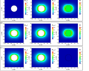
Appearance of ${\bf p}^{\rm sph,in}_{\rm sca}={\bf p}^{\rm pl}_{\rm sca}$ demonstrates that scattered fields for the plane and spherical dipolar incident waves differ from each other by the source-free fields only. Indeed, the total field distributions for planar and spherical dipole incident waves are exactly the same, while their scattered fields differ by the amplitude only, as shown in Fig. 1 (a) and (b) for a silver particle of $R=10$ nm embedded in SiO₂. As a result, the field difference plotted in Fig. 1 (c) demonstrates the source-free scattered fields accompanied by the trivial solution for the total field ${\bf E}$ and, hence, for the scattering current density ${\bf J}_{\rm sca}$.

VI Scattering of spherically outgoing fields

Now, let us separate the effects of source-free and current-sourced fields. As we discussed above, the source-free scattered fields mathematically appear as a part of the trivial solution of Maxwell’s equations, where they fully compensate a part of the incident fields. As the scattered fields are spherically outgoing, the compensated part of the incident field must be spherically outgoing as well. To demonstrate the purely source-free scattered fields, we consider scattering of the outgoing dipolar spherical field (see Appendices B for details):

$${\bf E}^{\rm sph,out}_{\rm inc}=\frac{-{\rm i}E_{0}}{2f_{\rm rad}(r)}[{\bf e}_{r}(2+{\rm i}f_{\rm rad}(r))\cos\theta+\hskip 28.45274pt$$

$${\bf e}_{\theta}(1-{\rm i}f_{\rm rad}(r))\sin\theta]\mathop{\rm e}\nolimits^{-{\rm i}\omega t}~{}~{}$$ (18)

that does not contain any spherically incoming component. After application of the boundary conditions, we obtain the following amplitudes of the scattered and internal fields:

$$\displaystyle A^{\rm sph,out}=A({\bf E}_{\rm inc}={\bf E}^{\rm sph,out}_{\rm inc})=\frac{{\rm i}}{2f_{\rm rad}(R)},$$ (19)

$$\displaystyle B^{\rm sph,out}=B({\bf E}_{\rm inc}={\bf E}^{\rm sph,out}_{\rm inc})=0,$$ (20)

revealing the nonzero source-free scattered field with the effective electric dipole moment

$${\bf p}^{\rm sph,out}_{\rm eff}=-{\bf e}_{z}\frac{2\pi\varepsilon_{0}\varepsilon_{e}R^{3}E_{0}}{{\rm i}f_{\rm rad}(R)}\mathop{\rm e}\nolimits^{-{\rm i}\omega t}$$ (21)

and the null scattering current with the electric dipole moment

$${\bf p}^{\rm sph,out}_{\rm sca}=0.$$ (22)

The solution obtained is trivial for electric field with the net zero total field ${\bf E}$ everywhere in space, as shown in Fig. 1 (c). This solution demonstrates the evident failure of the scattering current approach for description of such type of source-free scattered fields.

The failure of the scattering current approach for description of scattered fields comes from its limitation to electrodynamic formulation where any electromagnetic fields must have sources in terms of their currents. By rejecting source-free fields, the scattering current approach naturally fails for complete description of scattering problems where free incident fields are used. To be fully compliant with the electrodynamic formulation, the scattering current approach must eliminate the use of free fields, including the incident one. This requires Eq. (5) to be rewritten as follows:

$$\nabla\times\nabla\times{\bf E}-\omega^{2}\mu_{0}\varepsilon_{0}\varepsilon_{e}{\bf E}={\rm i}\omega\mu_{0}{\bf J}_{\rm sca},$$ (23)

where ${\bf J}_{\rm sca}$ is now appears the source of ${\bf E}$, not ${\bf E}_{\rm sca}$. According to this equation, ${\bf p}_{\rm sca}$ should be considered as the electric dipole moment of the total fields, not the scattered ones. Eventually, this clarifies the equality ${\bf p}^{\rm sph,in}_{\rm sca}={\bf p}^{\rm pl}_{\rm sca}$ observed for the plane and spherically incoming ${\bf E}_{\rm inc}$, whose total fields ${\bf E}$ are identical, as shown in Fig. 1.

Figure 2: Scattering and absorption cross-sections of silver nanoparticles of $R=10$ nm embedded in silicon dioxide as functions of the wavelength of incident plane waves. Total cross-sections are shown for comparison and calculated based on the Mie theory that includes all types of multipole fields. The dipolar contributions are calculated based on the electric dipole polarizabilities $\alpha^{\rm pl}_{\rm j=0}$ and $\alpha^{\rm pl}_{\rm j\neq 0}$.

VII Two types of scattered fields

With the revealed structure of scattered fields, we can reconsider the solution obtained for plane incident fields. The plane incident field given by Eq. (8) can be decomposed over dipolar spherically incoming (13) and outgoing (18) fields as follows:

$${\bf E}^{\rm pl}_{\rm inc}={\bf E}^{\rm sph,in}_{\rm inc}+{\bf E}^{\rm sph,out}_{\rm inc}.$$ (24)

As the dipolar spherically incoming incident field does not contain any spherically outgoing component that could be compensated with the scattered fields, the part ${\bf E}^{\rm sph,in}_{\rm inc}$ of the plane incident field ${\bf E}^{\rm pl}_{\rm inc}$ experiences purely current-sourced scattering. At the same time, the spherically outgoing part ${\bf E}^{\rm sph,out}_{\rm inc}$ of the plane incident field is fully compensated by the scattered fields and, thus, experiences purely current-free scattering. In other words, decomposition of the plane fields into spherically incoming and outgoing fields helps us split the effective electric dipole moment of the plane incident field into two fundamentally different moments:

$${\bf p}^{\rm pl}_{\rm eff}={\bf p}^{\rm pl}_{\rm j=0}+{\bf p}^{\rm pl}_{\rm j\neq 0}.$$ (25)

where

$$\displaystyle{\bf p}^{\rm pl}_{\rm j=0}={{\bf p}^{\rm sph,out}_{\rm eff}}={\bf e}_{z}\varepsilon_{0}\varepsilon_{e}\alpha^{\rm pl}_{\rm j=0}E_{0}\mathop{\rm e}\nolimits^{-{\rm i}\omega t},$$ (26)

$$\displaystyle{\bf p}^{\rm pl}_{\rm j\neq 0}={{\bf p}^{\rm sph,in}_{\rm eff}}={\bf e}_{z}\varepsilon_{0}\varepsilon_{e}\alpha^{\rm pl}_{\rm j\neq 0}E_{0}\mathop{\rm e}\nolimits^{-{\rm i}\omega t}$$ (27)

are the electric dipole moments of the current-free and current-sourced scattering given in terms of their polarizabilities

$$\displaystyle\alpha^{\rm pl}_{\rm j=0}=-\frac{2\pi R^{3}}{{\rm i}f_{\rm rad}(R)}=\frac{3{\rm i}\pi}{k_{e}^{3}},$$ (28)

$$\displaystyle\alpha^{\rm pl}_{\rm j\neq 0}=-\alpha^{\rm pl}_{\rm j=0}\frac{1+{\rm i}A_{\rm qs}f_{\rm rad}(R)}{1-{\rm i}A_{\rm qs}f_{\rm rad}(R)}.$$ (29)

This separation is further confirmed by Mie theory [23] and generalized Lorenz-Mie theory (see Appendix A) that provide the exact multipole solution for scattering of electromagnetic waves on a spherical particle, following which spherically outgoing parts of the incident fields experience current-free scattering for any polarization, orbital and azimuthal structure.

By interfering, ${\bf p}^{\rm pl}_{\rm j=0}$ and ${\bf p}^{\rm pl}_{\rm j\neq 0}$ make the resultant electric dipole moment ${\bf p}^{\rm pl}_{\rm eff}$ resonant and, hence, define all spectral peculiarities in the scattering and absorption cross-sections for deeply subwavelength spheres [1, 3, 2]:

$$\displaystyle\sigma_{\rm sca}^{\rm pl}=\frac{3\pi}{2k_{e}^{2}}\left|\frac{{\bf p}^{\rm pl}_{\rm eff}\cdot{\bf E}_{0}^{*}}{\varepsilon_{0}\varepsilon_{e}\alpha^{\rm pl}_{\rm j=0}|E_{0}|^{2}}\right|^{2},$$ (30)

$$\displaystyle\sigma_{\rm abs}^{\rm pl}=\frac{3\pi}{k_{e}^{2}}{\rm Re}\left(\frac{{\bf p}^{\rm pl}_{\rm eff}\cdot{\bf E}_{0}^{*}}{\varepsilon_{0}\varepsilon_{e}\alpha^{\rm pl}_{\rm j=0}|E_{0}|^{2}}\right)-\sigma_{\rm sca}^{\rm pl}.$$ (31)

For instance, the destructive interference of the two moments, ${\bf p}^{\rm pl}_{\rm j\neq 0}=-{\bf p}^{\rm pl}_{\rm j=0}$, results in the nonradiating states of purely electric dipole structure that do not require toroidal or any other higher-order moments. These states exist at either $k_{e}=0$ or $\varepsilon_{i}=\varepsilon_{e}$. The constructive interference of the two moments, ${\bf p}^{\rm pl}_{\rm j\neq 0}={\bf p}^{\rm pl}_{\rm j=0}$, results in the super-radiating state that require $\varepsilon_{i}=-2\varepsilon_{e}$.

Noteworthy that amongst the two electric dipole moments only the current-sourced one, ${\bf p}^{\rm pl}_{\rm j\neq 0}$, depends on the sphere permittivity and, thus, solely defines its effect on the scattering and absorption cross-sections. As $A_{\rm qs}$ is resonant to $\varepsilon_{i}$ given by the pole $(\varepsilon_{i}+2\varepsilon_{e})^{-1}$ in Eq. (11), the effect of $\varepsilon_{i}$ on the cross-sections differs inside the resonance and out of it.

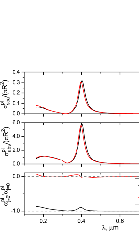
For large wavelength out of the resonance, when $|A_{\rm qs}|\sim 1$, the current-sourced electric dipole moment ${\bf p}^{\rm pl}_{\rm j\neq 0}\approx-{\bf p}^{\rm pl}_{\rm j=0}$. This regime, known as the Rayleigh scattering, is influenced by the nonradiating state with $k_{e}=0$. The above state is material-independent and common to all subwavelength particles. This regime features $\sigma_{\rm abs}^{\rm pl},\sigma_{\rm abs}^{\rm pl}\ll\pi R^{2}$ and can be seen in Fig. 2 for $R=10$ nm Ag nanoparticles embedded in SiO₂ at $\lambda>400$ nm when $|\varepsilon_{i}|>2\varepsilon_{e}$.

In the resonant wavelength range, where $|A_{\rm qs}|>1$, the current-sourced electric dipole moment deviates more from its destructive value $-{\bf p}^{\rm pl}_{\rm j=0}$, giving rise to stronger ${\bf p}^{\rm pl}_{\rm eff}$ and, hence, scattering and absorption. This regime is influenced by the super-radiating state and seen in Fig. 2 around the surface-plasmon-polariton resonance at $\lambda=$395 nm with the maximum scattering and absorption cross-sections of $0.3\pi R^{2}$ and $5.6\pi R^{2}$ when $\varepsilon_{i}\approx-2\varepsilon_{e}$.

For smaller wavelength out of the resonance, at which $|A_{\rm qs}|$ drops below 1, the destructive interference restores influenced by the nonradiating state with $\varepsilon_{i}=\varepsilon_{e}$. The corresponding anapole scattering features strong suppression of $\sigma_{\rm sca}^{\rm pl}$ and $\sigma_{\rm abs}^{\rm pl}$, as seen in Fig. 2 at $\lambda\approx$ 318 nm when $\varepsilon_{i}\approx\varepsilon_{e}$. Noteworthy that the quadratic dependence of $\sigma_{\rm sca}^{\rm pl}$ on ${\bf p}_{\rm eff}^{\rm pl}$ makes its drop dipper compared to $\sigma_{\rm abs}^{\rm pl}$ that features dominant linear dependence on ${\bf p}_{\rm eff}^{\rm pl}$. For instance, the anapole scattering shown in Fig. 2 experiences $\sim 500$ times reduction for $\sigma_{\rm sca}^{\rm pl}$ and only $\sim 40$ times for $\sigma_{\rm abs}^{\rm pl}$ with respect to their resonant values.

VIII Conclusion

In conclusion, classical scattering problems being the model tasks that use free electromagnetic fields for incident radiation inevitably face the issue of free scattered fields. This issue makes the conventional current moment analysis generally inapplicable to the scattered fields. As a result, the independent current-sourced and current-free field moments should be used instead. Together, the two moments completely define all the spectral features, as has been demonstrated in the paper for the classical case of dipole scattering by deeply subwavelength spherical particles.

Appendix A Generalized Lorenz-Mie theory

Generalized Lorenz-Mie theory describes scattering and absorption of free electromagnetic fields of arbitrary structure incident on a spherical particle [24, 25]. Following it, Maxwell’s equations

$$\displaystyle\nabla\times{\bf H}=\varepsilon_{0}\varepsilon\frac{{\rm\partial}{\bf E}}{{\rm\partial}t}+{\bf J},\quad\nabla\times{\bf E}=-\mu_{0}\frac{{\rm\partial}{\bf H}}{{\rm\partial}t},$$ (32)

can be solved for electromagnetic fields excited in domains with uniform dielectric permittivity $\varepsilon$ in terms of the transverse magnetic (TM) and transverse electric (TE) fields as follows [23, 26]:

$$\displaystyle{\bf H}=\left({\bf H}^{\rm TM}-{\rm i}\frac{\lambda}{2\pi}\sqrt{\frac{\varepsilon_{0}}{\mu_{0}}}\nabla\times{\bf E}^{\rm TE}\right)\mathop{\rm e}\nolimits^{-{\rm i}\omega t},$$ (33)

$$\displaystyle{\bf E}=\left({\bf E}^{\rm TE}+{\rm i}\frac{\lambda}{2\pi\varepsilon}\sqrt{\frac{\mu_{0}}{\varepsilon_{0}}}\nabla\times{\bf H}^{\rm TM}\right)\mathop{\rm e}\nolimits^{-{\rm i}\omega t},$$ (34)

where ${\bf H}^{\rm TM}$ and ${\bf E}^{\rm TE}$ are the amplitudes of the governing fields for the TM and TE polarizations. In the spherical geometry, the governing TM and TE fields can be decomposed over the vector spherical harmonics of different orbital and azimuthal indices $l,m$ [23, 26]:

$$\displaystyle{\bf H}^{\rm TM}=\sum_{l=0}^{\infty}\sum_{m=-l}^{l}\sum_{j=1}^{2}{H}_{lm}^{(j)}h_{l}^{(j)}(kr){\bf Y}_{lm}^{(3)}(\theta,\phi),$$ (35)

$$\displaystyle{\bf E}^{\rm TE}=\sum_{l=0}^{\infty}\sum_{m=-l}^{l}\sum_{j=1}^{2}{E}_{lm}^{(j)}h_{l}^{(j)}(kr){\bf Y}_{lm}^{(3)}(\theta,\phi).$$ (36)

In this decomposition, the angular dependence of the excited fields is fully given by the vector spherical harmonics [27]

$${\bf Y}_{lm}^{(3)}(\theta,\phi)={\bf e}_{\phi}\frac{{\rm\partial}Y_{lm}(\theta,\phi)}{{\rm\partial}\theta}-\frac{{\bf e}_{\theta}}{\sin\theta}\frac{{\rm\partial}Y_{lm}(\theta,\phi)}{{\rm\partial}\phi},$$ (37)

defined with

$$Y_{lm}(\theta,\phi)=\sqrt{\frac{2l+1}{4\pi}\frac{(l-m)!}{(l+m)!}}\,P_{l}^{m}(\cos\theta)\mathop{\rm e}\nolimits^{{\rm i}m\phi},$$ (38)

where $P_{l}^{m}(\cos\theta)$ are the associated Legendre polynomials, while the radial dependence is fully given by the spherical Hankel functions $h_{l}^{(1,2)}(kr)$ defined with $k=2\pi\sqrt{\varepsilon}/\lambda$. The amplitudes ${H}_{lm}^{(1,2)}$ and ${E}_{lm}^{(1,2)}$ are generally independent of each other and give all possible distributions of electromagnetic fields supported by Maxwell’s equations for uniform domains.

Depending on the spatial distribution, incident fields can possess any values of $[{H}_{lm}^{(1,2)}]_{\rm inc}$ and $[{E}_{lm}^{(1,2)}]_{\rm inc}$. Scattered fields, being spherically diverging, always feature $[{H}_{lm}^{(2)}]_{\rm sca}=0$ and $[{E}_{lm}^{(2)}]_{\rm sca}=0$, while $[{H}_{lm}^{(1)}]_{\rm sca}$ and $[{E}_{lm}^{(1)}]_{\rm sca}$ appear linear to the incident field amplitudes:

$$\displaystyle[{H}_{lm}^{(1)}]_{\rm sca}=-\sum_{j=1}^{2}a^{(j)}_{lm}[{H}_{lm}^{(j)}]_{\rm inc},$$ (39)

$$\displaystyle[{E}_{lm}^{(1)}]_{\rm sca}=-\sum_{j=1}^{2}b^{(j)}_{lm}[{E}_{lm}^{(j)}]_{\rm inc},$$ (40)

where the coefficients $a^{(1,2)}_{lm}$ and $b^{(1,2)}_{lm}$ give contributions of the TM and TE incident fields with different orbital and azimuthal structure to the scattered fields. As for internal fields, they always feature $[{H}_{lm}^{(2)}]_{\rm inc}=[{H}_{lm}^{(1)}]_{\rm inc}$ and $[{E}_{lm}^{(2)}]_{\rm inc}=[{E}_{lm}^{(1)}]_{\rm inc}$ for finiteness in the sphere’s center, $r=0$. Similarly to scattered fields, internal fields appear linear to $[{H}_{lm}^{(1,2)}]_{\rm inc}$ and $[{E}_{lm}^{(1,2)}]_{\rm inc}$:

$$\displaystyle[{H}_{lm}^{(1)}]_{\rm int}=\sum_{j=1}^{2}d^{(j)}_{lm}[{H}_{lm}^{(j)}]_{\rm inc},$$ (41)

$$\displaystyle[{E}_{lm}^{(1)}]_{\rm int}=\sum_{j=1}^{2}c^{(j)}_{lm}[{E}_{lm}^{(j)}]_{\rm inc},$$ (42)

where the coefficients $d^{(1,2)}_{lm}$ and $c^{(1,2)}_{lm}$ give the TM and TE contributions of the incident fields with different orbital and azimuthal structure to the internal fields.

Following the continuity of the tangential electric and magnetic fields on the particle surface $r=R$, the field coefficients given for spherically outgoing incident fields are

$$\displaystyle a^{(1)}_{lm}=b^{(1)}_{lm}=1,\quad c^{(1)}_{lm}=d^{(1)}_{lm}=0.$$ (43)

These coefficients correspond to the current-free scattered fields that appear as a part of the trivial solution of Maxwell’s equations for all polarizations, orbital and azimuthal compositions. As for spherically incoming incident fields, their contributions are size- and material-dependent following nontrivial solutions of Maxwell’s equations with nonzero polarization currents induced in the spherical particle:

$$\displaystyle a_{lm}^{(2)}=\frac{q_{i}\psi_{l}(q_{i})\zeta_{l}^{\prime}(q_{e})-q_{e}\zeta_{l}(q_{e})\psi_{l}^{\prime}(q_{i})}{q_{i}\psi_{l}(q_{i})\xi_{l}^{\prime}(q_{e})-q_{e}\xi_{l}(q_{e})\psi_{l}^{\prime}(q_{i})},$$ (44)

$$\displaystyle b_{lm}^{(2)}=\frac{q_{e}\psi_{l}(q_{i})\zeta_{l}^{\prime}(q_{e})-q_{i}\zeta_{l}(q_{e})\psi_{l}^{\prime}(q_{i})}{q_{e}\psi_{l}(q_{i})\xi_{l}^{\prime}(q_{e})-q_{i}\xi_{l}(q_{e})\psi_{l}^{\prime}(q_{i})},$$ (45)

$$\displaystyle c_{lm}^{(2)}=\frac{1}{2}\frac{q_{i}\psi_{l}(q_{e})\zeta_{l}^{\prime}(q_{e})-q_{i}\zeta_{l}(q_{e})\psi_{l}^{\prime}(q_{e})}{q_{e}\psi_{l}(q_{i})\xi_{l}^{\prime}(q_{e})-q_{i}\xi_{l}(q_{e})\psi_{l}^{\prime}(q_{i})},$$ (46)

$$\displaystyle d_{lm}^{(2)}=\frac{1}{2}\frac{q_{i}\zeta_{l}(q_{e})\xi_{l}^{\prime}(q_{e})-q_{i}\xi_{l}(q_{e})\zeta_{l}^{\prime}(q_{e})}{q_{i}\psi_{l}(q_{i})\xi_{l}^{\prime}(q_{e})-q_{e}\xi_{l}(q_{e})\psi_{l}^{\prime}(q_{i})},$$ (47)

where $\xi_{l}(q)=qh_{l}^{(1)}(q)$, $\zeta_{l}(q)=qh_{l}^{(2)}(q)$, $\psi_{l}(q)=[\xi_{l}(q)+\zeta_{l}(q)]/2$, are the Riccati–Bessel functions, with $q_{i}=k_{i}R$ and $q_{e}=k_{e}R$.

Appendix B Dipolar fields

In generalized Lorenz-Mie theory, the fields possesing a $z$-polarized electric dipole moment are given by the TM contributions with the orbital index $l=1$ and azimuthal index $m=0$:

$$\displaystyle{\bf H}^{\rm TM}_{\rm ED}=\sum_{j=1}^{2}{H}_{10}^{(j)}h_{1}^{(j)}(kr){\bf Y}_{10}^{(3)}(\theta,\phi).$$ (48)

Eventually, spatial distribution of electric field is given by

$${\bf E}_{\rm ED}={\rm i}\frac{\lambda}{2\pi\varepsilon}\sqrt{\frac{\mu_{0}}{\varepsilon_{0}}}\nabla\times{\bf H}^{\rm TM}_{\rm ED}\mathop{\rm e}\nolimits^{-{\rm i}\omega t}.$$ (49)

Applying Eq. (49) to the internal area of the sphere and assuming $|k_{i}|r\ll 1$, we get the field distribution used in Eq. (3) for the internal field excited inside the deeply subwavelegth particles:

$$\displaystyle{\bf E}_{\rm int}=C_{\rm int}({\bf e}_{r}\cos\theta-{\bf e}_{\theta}\sin\theta)\mathop{\rm e}\nolimits^{-{\rm i}\omega t}+O(|k_{i}r|^{2})~{}~{}$$ (50)

with the field amplitude defined as

$$C_{\rm int}=-{\rm i}\left(\frac{4}{3\pi}\frac{\mu_{0}}{\varepsilon_{0}\varepsilon_{i}}\right)^{1/2}{H}_{10}^{(1)}.$$ (51)

For the external area of the sphere, we separately consider spherically outgoing and incoming fields. Under $|k_{e}|r\ll 1$, Eq. (49) gives us the following distribution for the outgoing dipolar field

$$\displaystyle{\bf E}_{\rm ext}^{\rm sph,out}=-{\rm i}\frac{C_{\rm ext}^{\rm sph,out}}{2f_{\rm rad}(r)}[{\bf e}_{r}(2+k_{e}^{2}r^{2}+{\rm i}f_{\rm rad}(r))\cos\theta+~{}~{}$$

$$\displaystyle{\bf e}_{\theta}\left(1-\frac{k_{e}^{2}r^{2}}{2}-{\rm i}f_{\rm rad}(r)\right)\sin\theta]\mathop{\rm e}\nolimits^{-{\rm i}\omega t}+O(|k_{e}r|^{\frac{1}{2}})~{}~{}~{}$$ (52)

with the amplitude of

$$C_{\rm ext}^{\rm sph,out}=-{\rm i}\left(\frac{4}{3\pi}\frac{\mu_{0}}{\varepsilon_{0}\varepsilon_{e}}\right)^{1/2}{{H}_{10}^{(1)}}.$$ (53)

This field was used in Eq. (2) for the scattered field and in Eq. (18) for the spherically outgoing incident field, where we left only the leading real and imaginary terms. As for spherically incoming external fields under $|k_{e}|r\ll 1$, Eq. (49) results in

$$\displaystyle{\bf E}_{\rm ext}^{\rm sph,in}={\rm i}\frac{C_{\rm ext}^{\rm sph,in}}{2f_{\rm rad}(r)}[{\bf e}_{r}(2+k_{e}^{2}r^{2}-{\rm i}f_{\rm rad}(r))\cos\theta+~{}~{}~{}$$

$$\displaystyle{\bf e}_{\theta}\left(1-\frac{k_{e}^{2}r^{2}}{2}+{\rm i}f_{\rm rad}(r)\right)\sin\theta]\mathop{\rm e}\nolimits^{-{\rm i}\omega t}+O(|k_{e}r|^{\frac{1}{2}})~{}~{}~{}~{}$$ (54)

where the field amplitude $C_{\rm ext}^{\rm sph,in}$ is given by

$$C_{\rm ext}^{\rm sph,in}=-{\rm i}\left(\frac{4}{3\pi}\frac{\mu_{0}}{\varepsilon_{0}\varepsilon_{e}}\right)^{1/2}{{H}_{10}^{(2)}}.$$ (55)

This distirbution was used in Eq. (13) for the spherically incoming incident field, where we left the dominant real and imaginary terms. Regarding the plane field used in Eq. (8) for ${\bf E}^{\rm pl}_{\rm inc}$, it is given by the superposition of spherically incoming ${\bf E}_{\rm ext}^{\rm sph,in}$ and outgoing ${\bf E}_{\rm ext}^{\rm sph,out}$ fields taken with equal amplitudes ${H}_{10}^{(1)}$ and ${H}_{10}^{(2)}$:

$$\displaystyle{\bf E}_{\rm ext}^{\rm pl}=C_{\rm ext}^{\rm pl}({\bf e}_{r}\cos\theta-{\bf e}_{\theta}\sin\theta)\mathop{\rm e}\nolimits^{-{\rm i}\omega t}+O(|k_{e}r|^{2}),~{}~{}$$ (56)

where the resultant field amplitude is

$$C_{\rm ext}^{\rm pl}=-{\rm i}\left(\frac{4}{3\pi}\frac{\mu_{0}}{\varepsilon_{0}\varepsilon_{e}}\right)^{1/2}{H}_{10}^{(1)}.$$ (57)

References

• [1] L. D. Landau and E. M. Lifshitz, Electrodynamics of Continuous Media, 2nd ed. (Butterworth-Heinemann, 1984).
• [2] J. D. Jackson, Classical Electrodynamics, 3rd ed. (Wiley, 1999).
• [3] C. F. Bohren and D. R. Huffman, Absorption and Scattering of Light by Small Particles, 3rd ed. (Wiley-VCH, 1998).
• [4] C. F. Bohren, Am. J. Phys. 51, 323–327 (1983).
• [5] A. E. Miroshnichenko et al., Nat. Commun. 6, 8069 (2015).
• [6] B. Luk’yanchuk, R. Paniagua-Dominguez, A. I. Kuznetsov, A. E. Miroshnichenko and Y. S. Kivshar, Phil. Trans. R. Soc. A 375, 20160069 (2017).
• [7] P. Grahn, A. Shevchenko and M. Kaivola, New J. Phys. 14, 093033 (2012).
• [8] Y. A. Akimov, Plasmonics 7, 495–500 (2012).
• [9] K. Kolwas K and A. Derkachova, J. Quant. Spectrosc. Radiat. Transf. 114, 45–55 (2013).
• [10] B. T. Draine, Astrophys. J. 333, 848 (1988).
• [11] B. T. Draine and P. J. Flatau, J. Opt. Soc. Am. A 11, 1491 (1994).
• [12] E. Zubko et al., Appl. Opt. 49, 1267 (2010).
• [13] A. B. Evlyukhin, C. Reinhardt and B. N. Chichkov, Phys. Rev. B 84, 235429 (2011).
• [14] A. B. Evlyukhin, T. Fischer, C. Reinhardt and B. N. Chichkov, Phys. Rev. B 94, 205434 (2016).
• [15] I. Fernandez-Corbaton, S. Nanz and C. Rockstuhl, Sci. Rep. 7 7527, (2017).
• [16] A. B. Evlyukhin and B. N. Chichkov, Phys. Rev. B 100, 125415 (2019).
• [17] E. A. Gurvitz, K. S. Ladutenko, P. A. Dergachev, A. B. Evlyukhin, A. E. Miroshnichenko and A. S. Shalin, Laser Photonics Rev. 13, 1800266 (2019).
• [18] T. Liu, R. Xu, P. Yu, Z. Wang and J. Takahara, Nanophotonics 9, 1115–1137 (2020).
• [19] R. Alaee, A. Safari, V. Sandoghdar and R. W. Boyd, Phys. Rev. Research 2, 043409 (2020).
• [20] V. A. Zenin et al., ACS Photonics 7, 1067–1075 (2020).
• [21] A. A. Basharin, E. Zanganeh, A. K. Ospanova, P. Kapitanova and A. B. Evlyukhin, Phys. Rev. B 107, 155104 (2023).
• [22] A. Ospanova, M. Cojocari and A. Basharin, Phys. Rev. B 107, 035156 (2023).
• [23] Y. A. Akimov, arXiv:2401.04146.
• [24] G. Gouesbet, B. Maheu and G. Gréhan, J. Opt. Soc. Am. A 5 1427–1443 (1988).
• [25] G. Gouesbet and G. Gréhan, “Generalized Lorenz-Mie theories”. (Springer, 2011).
• [26] Y. A. Akimov, “Plasmonic properties of metal nanostructures”, in Plasmonic Nanoelectronics and Sensing (H.-S. Chu, E.-P. Li, eds). (Cambridge University Press, 2014).
• [27] R. G. Barrera, G. A. Estévez, and J. Giraldo, Eur. J. Phys. 6 287–294 (1985).