Abstract

Morden deep ensembles technique achieves strong uncertainty estimation performance by going through multiple forward passes with different models. This is at the price of a high storage space and a slow speed in the inference (test) time. To address this issue, we propose Density-Regression, a method that leverages the density function in uncertainty estimation and achieves fast inference by a single forward pass. We prove it is distance aware on the feature space, which is a necessary condition for a neural network to produce high-quality uncertainty estimation under distribution shifts. Empirically, we conduct experiments on regression tasks with the cubic toy dataset, benchmark UCI, weather forecast with time series, and depth estimation under real-world shifted applications. We show that Density-Regression has competitive uncertainty estimation performance under distribution shifts with modern deep regressors while using a lower model size and a faster inference speed.

1 Introduction

Improving the uncertainty quality of Deep Neural Network (DNN)is crucial in high-stakes Artificial Intelligence (AI)applications in real-world applications (Tran et al., 2022; Nado et al., 2021). For example, in regression tasks like predicting temperature in weather forecasts, depth estimation in medical diagnosis, and autonomous driving, accurate uncertainty hinges on the calibration property (Guo et al., 2017), i.e., the frequency of realizations below specific quantiles must match the respective quantile levels (Kuleshov et al., 2018). Furthermore, the forecast must exhibit an appropriate level of sharpness, i.e., concentrated around the realizations and leveraging the information in the inputs effectively (Kuleshov and Deshpande, 2022).

Method	$\begin{matrix}\text{Uncertainty}\\ \text{quality}\end{matrix}$	$\begin{matrix}\text{Test-time}\\ \text{efficiency}\end{matrix}$	$\begin{matrix}\text{Without prior}\\ \text{requirement}\end{matrix}$
Deterministic	✗	✓	✓
Bayesian	✓	✓	✗
Ensembles	✓	✗	✓
Ours	✓	✓	✓

Table 1: A comparison between methods in terms of uncertainty quality (calibration & sharpness), test-time efficiency (lightweight & fast), and whether pre-defined prior hyper-parameters are required.

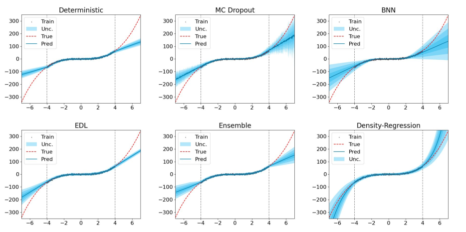
Figure 1: Predictive distributions for the toy dataset $y=x^{3}+\epsilon$, $\epsilon\sim\mathcal{N}(0,3^{2})$. The gray dots in the area between two vertical dashed lines represent observations in training, the red dashed line represents the true data-generating function, and the blue line represents the mean predictions in which blue areas correspond to $\pm 3$ standard deviation around the mean. Our Density-Regression achieves distance awareness and, therefore, can improve distribution calibration by confident & sharp predictions on IID training data and decreased certainty and sharpness when the OOD data is far from the training set. A quick demo is available at this Google Colab link.

However, modern Deterministic DNN is often over-confident, especially under distribution shifts in real-world applications (Tran et al., 2022; Minderer et al., 2021; Bui et al., 2021). For instance, a Deterministic DNN trained with in-door images but deployed in outdoor scenes will result in sharp but un-calibrated predictions. Sampling-based approaches such as Gaussian Process (GP), Bayesian Neural Network (BNN), Monte-Carlo (MC) Dropout, and Deep Ensembles can reduce over-confidence (Koh et al., 2021; Lakshminarayanan et al., 2017; Chen et al., 2016). However, such approaches usually have high computational demands by using multiple forward passes (or merging predictions from multiple models with Ensembles) at inference (test) time.

To mitigate the inefficiency issue, sampling-free approaches, including Quantile Regression (Romano et al., 2019), Spectral-normalized Neural Gaussian Process (SNGP) (Liu et al., 2020), Deterministic Uncertainty Estimation (DUE) (van Amersfoort et al., 2022), and closed-form posteriors in Bayesian inference (e.g., Evidential Deep Learning (EDL) (Sensoy et al., 2018), Natural Posterior Network (NatPN) (Charpentier et al., 2022)), have been proposed. The Bayesian approach, however, requires pre-defined prior hyper-parameters, which are often sensitive and unknown in the real world. In addition, these aforementioned approaches still under-perform relative to sampling-based techniques and require a higher computational demand than the Deterministic DNN (e.g., Tab. 1).

Towards a model enhancing uncertainty quality, test-time efficiency, and not requiring any pre-defined prior hyper-parameter, we propose Density-Regression. Our framework includes three main components: a feature extractor, a density function on feature space, and a regressor. The key component is the density function. By combining its likelihood value as an in-out-distribution detector on the feature space, the regressor achieves improved predictive uncertainty under distribution shifts. At the same time, it preserves the level of test-time efficiency of Deterministic DNN.

Our contributions can be summarized as:

1. We introduce Density-Regression, a novel deterministic framework that improves DNN uncertainty by a combination of density function with the regressor. Density-Regression is fast and lightweight. It is able to produce reliable predictions under distribution shifts, and can be implemented efficiently and easily across DNN architectures.

2. We develop a rigorous theoretical connection for our framework, and formally prove that it is distance-aware on the feature space, i.e., its associated uncertainty metrics are monotonic functions of feature distance metrics. This is an important property to help DNN improve calibration, however, it is often not guaranteed for typical DNN models (Liu et al., 2020) (e.g., Fig. 1).

3. We empirically show our framework achieves competitive uncertainty estimation quality with State-of-the-art (SOTA)across different tasks, including the cubic dataset, time-series weather forecast, UCI benchmark dataset, and monocular depth estimation. Importantly, it requires only a single forward pass and a lightweight feature density function. Therefore, it has fewer parameters and is much faster than other baselines at test time.

2 Background

2.1 Preliminaries

Notation and Problem setting. Let $\mathcal{X}$ and $\mathcal{Y}$ be the sample and label space. Denote the set of joint probability distributions on $\mathcal{X}\times\mathcal{Y}$ by $\mathcal{P}_{\mathcal{X}\times\mathcal{Y}}$. A dataset is defined by a joint distribution $\mathbb{P}(x,y)\in\mathcal{P}_{\mathcal{X}\times\mathcal{Y}}$, and let $\mathcal{P}$ be a measure on $\mathcal{P}_{\mathcal{X}\times\mathcal{Y}}$, i.e., whose realizations are distributions on $\mathcal{X}\times\mathcal{Y}$. Denote the training set by $D_{s}=\{(x_{s}^{i},y_{s}^{i})\}_{i=1}^{n_{s}}$, where $n_{s}$ is the number of data points in $D_{s}$, s.t., $(x_{s},y_{s})\sim\mathbb{P}_{s}(x,y)$ and $\mathbb{P}_{s}(x,y)\sim\mathcal{P}$. In the standard learning setting, a learning model that is only trained on $D_{s}$, arrives at a good generalization performance on the test set $D_{t}=\{(x_{t}^{i},y_{t}^{i})\}_{i=1}^{n_{t}}$, where $n_{t}$ is the number of data points in $D_{t}$, s.t., $(x_{t},y_{t})\sim\mathbb{P}_{t}(x,y)$ and $\mathbb{P}_{t}(x,y)\sim\mathcal{P}$. In the Independent-identically-distributed (IID)setting, $\mathbb{P}_{t}(x,y)$ is similar to $\mathbb{P}_{s}(x,y)$, and let us use $\mathbb{P}_{iid}(x,y)$ to represent the IID test distribution. In contrast, $\mathbb{P}_{t}(x,y)$ is different with $\mathbb{P}_{s}(x,y)$ if $D_{t}$ is Out-of-Distribution (OOD)data, and let us use $\mathbb{P}_{ood}(x,y)$ to represent the OOD test distribution.

Deterministic Regression. In the regression setting of representation learning, we predict a target $y\in\mathcal{Y}$, where $\mathcal{Y}=\mathbb{R}$ is continuous by using a forecast $h=g\circ f$ which composites a features extractor $f:\mathcal{X}\rightarrow\mathcal{Z}$, where $\mathcal{Z}$ is feature space, a regressor $g:\mathcal{Z}\rightarrow\mathcal{Y}$ which outputs a predicted output over $\mathcal{Y}$. In Deterministic DNN, we often aim to learn a function $h$ by minimizing the Mean Squared Error

$$\min_{\theta_{g,f}}\left\{\mathbb{E}_{(x,y)\sim D_{s}}\left[\frac{1}{2}||y-g(f(x))||^{2}\right]\right\},$$ (1)

where $\theta_{g,f}$ is the parameter of encoder $f$ and regressor $g$. The model $h$ is optimized such that it can learn the average correct answer for a given input. Yet, there is no uncertainty estimation in this model when making the prediction (Chua et al., 2018; Tran et al., 2020).

Deterministic Gaussian DNN. To tackle this issue, one probabilistic approach is based on the assumption that the true label $y$ is distributed according to a normal distribution with a true mean $\mu(x)$ and some noise with the variance $\sigma^{2}(x)$ (Chua et al., 2018). Under this assumption, we can simplify the model to a probabilistic function $h$ to infer $(\mu,\sigma^{2})$ by making $g:\mathcal{Y}\rightarrow\mathbb{R}^{2}$, then optimize function $h$ by Maximum Likelihood Estimation (MLE)

$$\min_{\theta_{g,f}}\{\mathbb{E}_{(x,y)\sim D_{s}}[-\log p\left(y|g(f(x))\right)$$ (2)

$$:=\frac{1}{2}\log(2\pi\sigma^{2})+\frac{(y-\mu)^{2}}{2\sigma^{2}}]\}.$$

This approach, however, only helps the model $h$ provide data uncertainty when making predictions since it estimates the underlying noise in the data (i.e., aleatoric uncertainty), and the model uncertainty (i.e., epistemic uncertainty) is ignored (Tran et al., 2020).

Sampling-based Regression. The sampling-based approaches, i.e., make an inference by multiple forward passes (or merging predictions from multiple models), such as BNN, MC Dropout, and Deep Ensembles can model the model uncertainty by predicting

$$\mu(x)=\frac{1}{M}\sum_{i=1}^{M}\mu_{\theta_{i}}(x),$$ (3)

$$\sigma^{2}(x)=\frac{1}{M}\sum_{i=1}^{M}\left[\left(\mu(x)-\mu_{\theta_{i}}(x))^{2}+\sigma^{2}_{\theta_{i}}(x\right)\right],$$ (4)

where $\theta_{i}$ represents $i$-th model’s parameters. However, this approach struggles with computational cost by requiring multiple (i.e., $M$) model inferences.

2.2 Evaluating Uncertainty

Calibrated Regression. First, we present the definition of distribution calibration for the forecast $h$ under the regression setting by:

Definition 2.1.

(Gneiting et al., 2007) A forecast $h$ is said to be distributional calibrated if and only if

$$\mathbb{P}(Y\leq F_{x}^{-1}(p))=p,\forall p\in[0,1],$$ (5)

where we use $F_{x}:\mathcal{Y}\rightarrow[0,1]$ to denote the CDF of forecast $h(x)$ at $x$, hence $F_{i}^{-1}:[0,1]\rightarrow\mathcal{Y}$ means the quantile function $F_{i}^{-1}(p)=\inf\{y:p\leq F_{i}(y)\}$.

Intuitively, this means that a $p$ confidence interval contains the target $y$ $p$ of the time. This definition also implies that $\left(\sum_{i=1}^{n}\mathbb{I}\{F_{i}^{-1}(p_{1})\leq y_{i}\leq F_{i}^{-1}(p_{2})\}\right)/n\rightarrow p_{2}-p_{1}$, for all $p_{1},p_{2}\in[0,1]$ as $n\rightarrow\infty$. Under this confidence intervals intuition, Kuleshov et al. (2018) propose to measure the calibration error as a numerical score describing the quality of forecast calibration

$$cal(\{F_{i},y_{i}\}_{i=1}^{n})$$

$$:=\sum_{j=1}^{m}\left(p_{j}-\frac{\left|\{y_{i}|F_{i}(y_{i})\leq p_{j},i=1,\cdots,n\}\right|}{n}\right)^{2},$$ (6)

for each threshold $p_{j}$ from the chosen of $m$ confidence level $0\leq p_{1}<p_{2}<\cdots<p_{m}\leq 1$.

Sharpness. Calibration, however, is only a necessary condition for good uncertainty estimation. For example, a well-calibrated model could still have large confidence intervals, which is inherently less useful than a well-calibrated one with small confidence intervals. Therefore, another condition is that the forecast $h$ must also be sharp. Intuitively, this means that the confidence intervals should be as tight as possible, i.e., $var(F_{i})$ of the random variable whose CDF is $F_{i}$ to be small. Formally, the sharpness score (Tran et al., 2020) follows

$$sha(F_{1},\cdots,F_{n}):=\sqrt{\frac{1}{n}\sum_{i=1}^{n}var(F_{i})}.$$ (7)

Distance Awareness. One of the approaches to help the Deterministic Gaussian DNN provide model uncertainty is making it achieve distance awareness. This is an important property to improve model uncertainty under distributional shifts (Liu et al., 2020; van Amersfoort et al., 2022; Bui and Liu, 2024). It was introduced by Liu et al. (2020), and on the feature space $\mathcal{Z}$, we can define distance awareness as follows:

Definition 2.2.

The forecast $h(x_{t})$ on the new test feature $z_{t}=f(x_{t})$, is said to be feature distance-aware if there exists $u(z_{t})$, a summary statistics of $h(x_{t})$, that quantifies model uncertainty (e.g., entropy, predictive variance, etc.) and reflects the distance between $z_{t}$ and the features random variable on the training data $Z_{s}$ w.r.t. a metric $\left\|\cdot\right\|_{\mathcal{Z}}$, i.e., $u(z_{t}):=v(d(z_{t},Z_{s}))$, where $v$ is a monotonic function and $d(z_{t},Z_{s}):=\mathbb{E}\left\|z_{t}-Z_{s}\right\|_{\mathcal{Z}}$ is the distance between $z_{t}$ and $Z_{s}$.

Following Def. 2.2, if a model achieves the distance-aware property, model uncertainty quality would be improved and the over-confidence issues of current DNN on OOD would be reduced. While, at the same time, it will still preserve certainty predictions for the IID test example, suggesting calibration and sharpness improvement.

2.3 Test-time Efficiency

Latency. To deploy in real-world applications, a necessary condition is that the model must infer fast at the test-time. This is especially important in high-stakes applications such as autonomous driving when the car needs to react in sudden circumstances.

Parameters. Additionally, to make the model scalable, the model also needs to be as lightweight as possible to be installed with low-resource hardware. That said, current SOTA sampling-based approaches that can improve uncertainty quantification are still struggling with these two criteria (Tran et al., 2022; Nado et al., 2021; Bui and Liu, 2024).

3 Density-Regression

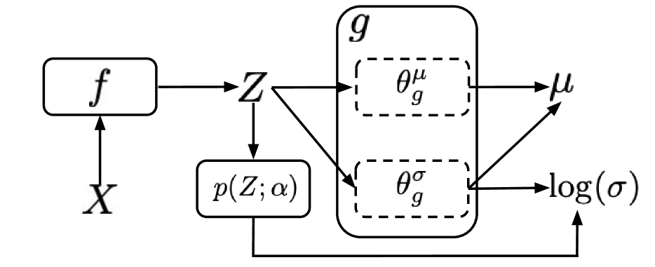
Figure 2: The overall architecture of Density-Regression, including encoder $f$, regressor $g$, and density function $p(Z;\alpha)$. Solid rectangle boxes represent these functions. Dashed rectangle boxes represent function weights. Three training steps and inference process follow Alg. 1

.

3.1 Exponential Family Distribution

To improve the uncertainty quality and test-time efficiency of DNN in regression under distribution shifts, we propose the Density-Regression framework in Fig. 2. First, recall that when $\mathcal{Y}$ is the label space and $\Phi(x,y)$ is the sufficient statistic of the joint distribution $\mathbb{P}(x,y)$ associated with $(x,y)\in\mathcal{X}\times\mathcal{Y}$, from Lemma A.1 in our Appendix A, we have the predictive distribution $p(y|x;\theta)$ follows

$$p(y|x;\theta)=\frac{\exp(\eta(\theta_{g})^{\top}\Phi(f(x),y))}{\int_{y^{\prime}\in\mathcal{Y}}\exp\left(\eta(\theta_{g})^{\top}\Phi(f(x),y^{\prime})\right)dy^{\prime}},$$ (8)

where $\eta$ is the natural function for the parameter $\theta$, $\theta=(\theta_{g},\theta_{f})$ is obtained by maximizing the MLE w.r.t. the conditional log-likelihood

$$\theta=\underset{\theta}{\arg\max}\mathbb{E}_{x,y\sim p(x,y)}[\log p(y|x;\theta)].$$ (9)

Motivated by the idea of using the density function to improve uncertainty estimation of DNN under distribution shifts (Bui and Liu, 2024; Charpentier et al., 2020; Kuleshov and Deshpande, 2022), in this paper, we integrate the density function into our Density-Regression’s framework by

$$p(y|x;\theta)=\frac{\exp\left(-p(z;\alpha)\theta_{g}^{\top}\Phi(z,y)\right)}{\int_{y^{\prime}\in\mathcal{Y}}\exp\left(-p(z;\alpha)\theta_{g}^{\top}\Phi(z,y^{\prime})\right)dy^{\prime}},$$ (10)

where $z=f(x)$ and the density function $p(z;\alpha)\in(0,\infty]$. The density $p(z;\alpha)$ modulates the distribution’s certainty. When the density goes to zero, the estimator $p(y|x;\theta)$ becomes uncertain. As the density goes toward infinity, the estimator converges to a deterministic point estimate. When Density-Regression follows a Gaussian distribution, we obtain the mean and variance by the following theorem:

Theorem 3.1.

If the predictive distribution follows Eq. 10 and the sufficient statistic has the form $\Phi(z,y)=\begin{bmatrix}zy^{2}&y^{2}&2zy&2y&z&1\end{bmatrix},$ then Density-Regression has the conditional Gaussian distribution as follows $p(y|x;\theta)\sim\mathcal{N}(\mu(x,\theta),\sigma^{2}(x,\theta)),$ where

$$\mu(x,\theta)=-\left(\theta_{g}^{\sigma}\begin{bmatrix}z\\ 1\end{bmatrix}\right)^{-1}\left(\theta_{g}^{\mu}{\begin{bmatrix}z\\ 1\end{bmatrix}}\right),$$

$$\sigma^{2}(x,\theta)=\left(2\cdot p(z;\alpha)\theta_{g}^{\sigma}\begin{bmatrix}z\\ 1\end{bmatrix}\right)^{-1},$$

where $z=f(x)$ and $\theta_{g}^{\mu}$ and $\theta_{g}^{\sigma}$ are the parameters (model weights) of the regressor $g$, i.e., $(\theta_{g}^{\mu},\theta_{g}^{\sigma})=\theta_{g}$ . The proof is in Apd. A.2.

The mean and variance in Theorem 3.1 are hard to optimize with MLE since they are undefined for non-positive $\theta_{g}^{\sigma}\begin{bmatrix}z,1\end{bmatrix}^{\top}$. To avoid this issue, we can rewrite the mean and the variance by the Corollary below:

Corollary 3.2.

Given the mean and variance in Theorem 3.1, we can rewrite as follows

$$\mu(x,\theta)=\sigma^{2}(z,\theta)\left(-2\cdot p(z;\alpha)\theta_{g}^{\mu}{\begin{bmatrix}z\\ 1\end{bmatrix}}\right),$$

$$\sigma^{2}(x,\theta)=\exp\left(-\frac{1}{2}\left[\log(2)+\log(p(z;\alpha))+\theta_{g}^{\sigma}\begin{bmatrix}z\\ 1\end{bmatrix}\right]\right)^{2}$$

, where $z=f(x)$. The proof is in Apd. A.3.

Corollary 3.2 gives a defined mean and variance formulation for every $\theta_{g}^{\sigma}\begin{bmatrix}z,1\end{bmatrix}^{\top}\in\mathbb{R}$ such that they can be easily optimized with MLE.

3.2 Training and Inference Process

Given these aforementioned results, we next present the training and inference of our framework:

Training. In the first training step, we optimize the model by using Empirical Risk Minimization (ERM) (Vapnik, 1998) with training data $D_{s}$, i.e., we do MLE

$$\min_{\theta_{g,f}}\left\{\mathbb{E}_{(x,y)\sim D_{s}}\left[\frac{1}{2}\log(2\pi\sigma_{o}^{2}(x,\theta))+\frac{(y-\mu_{o}(x,\theta))^{2}}{2\sigma_{o}^{2}(x,\theta)}\right]\right\}$$ (11)

, where $\mu_{o}(x,\theta),\sigma_{o}^{2}(x,\theta)$ follows Corollary 3.2 without the density function $p(z;\alpha)$, i.e.,

$$\mu_{o}(x,\theta)=\sigma_{o}^{2}(z,\theta)\left(-2\cdot\theta_{g}^{\mu}{\begin{bmatrix}z\\ 1\end{bmatrix}}\right),$$ (12)

$$\sigma_{o}^{2}(x,\theta)=\exp\left(-\frac{1}{2}\left[\log(2)+\theta_{g}^{\sigma}\begin{bmatrix}z\\ 1\end{bmatrix}\right]\right)^{2},$$ (13)

where $z=f(x)$.

After that, we freeze the parameter $\theta_{f}$ of $f$ to estimate the density on the feature space $\mathcal{Z}$ by positing a statistical model for $p(Z;\alpha)$ with Normalizing-Flows (Dinh et al., 2017) since it is provable (in terms of Lemma 3.4), simple, and provides exact log-likelihood (Charpentier et al., 2022). Specifically, we optimize by using MLE w.r.t. the logarithm as follows

$$\max_{\alpha}\{\mathbb{E}_{z=f(x)\sim D_{B}}[\log(p(z;\alpha))$$

$$:=\log(p(t;\alpha))+\log\left|\det\left(\frac{\partial t}{\partial z}\right)\right|]\},$$ (14)

where random variable $t=s_{\alpha}(f(x))$ and $s$ is a bijective differentiable function. It is worth noticing that $p(Z;\alpha)$ can be any other density function (e.g., Kernel density estimation, Gaussian mixture models, etc.).

Finally, we combine our model with the likelihood value of the density function $p(Z;\alpha)$ by re-updating the weight of classifier $g$, i.e., $\theta_{g}$ via optimizing

$$\min_{\theta_{g}}\left\{\mathbb{E}_{(x,y)\sim D_{s}}\left[\frac{1}{2}\log(2\pi\sigma^{2}(x,\theta))+\frac{(y-\mu(x,\theta))^{2}}{2\sigma^{2}(x,\theta)}\right]\right\}$$ (15)

, where $\mu(x,\theta)$ and $\sigma^{2}(x,\theta)$ follows Corollary 3.2.

Inference. After completing the training process, for a new input $x_{t}$ at the test-time, we perform prediction by combining the density function on feature space $p(z_{t};\alpha)$ following Corollary 3.2. The pseudo-code for the training and inference processes of our proposed framework is presented in Algorithm 1 and the demo notebook code is in Apd. B.3.

Algorithm 1 Training and Inference (code is in Apd. B.3)

  Training Input: Dataset $D_{s}$, encoder $f$, density $p(f(X);\alpha)$, regressor $g$ with $\theta_{g}=(\theta_{g}^{\sigma},\theta_{g}^{\mu})$, learning rate $\eta$, batch-size $B$ 

  for $e=1\rightarrow\text{epochs}$ do

     Sample $(x,y)\in D_{B}$ with a mini-batch $B$ for $D_{s}$ 

     Set $\mu_{o}(x,\theta)$ and $\sigma_{o}^{2}(x,\theta)$ following Eq. 12 and Eq. 13

     Update $\theta_{g,f}$ as:

     $\theta_{g,f}-\eta\nabla_{\theta_{g,f}}\mathbb{E}_{(x,y)}\left[\frac{1}{2}\log(2\pi\sigma_{o}^{2}(x,\theta))+\frac{(y-\mu_{o}(x,\theta))^{2}}{2\sigma_{o}^{2}(x,\theta)}\right]$ 

  end for

  for $e=1\rightarrow\text{train-density epochs}$ do

     Sample $x\in D_{B}$ with a mini-batch $B$ for $D_{s}$ 

     Update $\alpha$ as:

     $\alpha-\eta\nabla_{\alpha}\mathbb{E}_{z=f(x)}\left[-\log(p(t;\alpha))-\log\left|\det\left(\frac{\partial t}{\partial z}\right)\right|\right]$

  end for

  for $e=1\rightarrow\text{epochs}$ do

     Sample $(x,y)\in D_{B}$ with a mini-batch $B$ for $D_{s}$ 

     Set $\sigma^{2}(x,\theta)$ and $\mu(x,\theta)$ following Corollary 3.2

     Update $\theta_{g}$ as:

     $\theta_{g}-\eta\nabla_{\theta_{g}}\mathbb{E}_{(x,y)}\left[\frac{1}{2}\log(2\pi\sigma^{2}(x,\theta))+\frac{(y-\mu(x,\theta))^{2}}{2\sigma^{2}(x,\theta)}\right]$ 

  end for

  Inference Input: Test sample $x_{t}$ 

  Set $\sigma^{2}(x_{t},\theta)$ and $\mu(x_{t},\theta)$ following Corollary 3.2

  Predict $\hat{y}_{t}\sim\mathcal{N}(\mu(x_{t},M);\sigma^{2}(x_{t},M))$ 

Remark 3.3.

(Computational efficiency at test-time) Corollary 3.2 shows that the complexity of Density-Regression at test-time is only $\mathcal{O}(1)$ by requiring only a single forward pass. Meanwhile, the sampling-based approach is $\mathcal{O}(M)$, where $M$ is the number of sampling times. Compared with Deterministic Gaussian DNN, ours computation only needs to additionally compute $p(z_{t};\alpha)$, therefore, only higher than Deterministic Gaussian DNN by the additional parameter $\alpha$ and the latency of $p(z_{t};\alpha)$. This number is often very small in practice by Fig. 5 (a) and Fig. 5 (b).

3.3 Theoretical Analysis

Intuitively, the predictive distribution of Density-Regression in Corollary 3.2 leads to reasonable uncertainty estimation for the two limit cases of strong IID and OOD data. In particular, for very unlikely OOD data, i.e., $d(z_{t},Z_{s})\rightarrow\infty$, the prediction become uncertain. Conversely, for very likely IID data, i.e., $d(z_{t},Z_{s})\rightarrow 0$, the prediction converges to a deterministic point estimate. We formally show this property below:

Let us recall a Lemma when $p(Z;\alpha)$ is a Normalizing-Flows model (Papamakarios et al., 2021):

Lemma 3.4.

(Lemma 5 (Charpentier et al., 2022)) If $p(Z;\alpha)$ is parametrized with a Gaussian Mixture Model (GMM) or a radial Normalizing-Flows, then $\lim_{d(z_{t},Z_{s})\rightarrow\infty}p(z_{t};\alpha)\rightarrow 0$.

Based on Lemma 3.4, we obtain the following results:

Theorem 3.5.

Density-Regression converges to a deterministic point estimate, i.e., $\sigma^{2}(x_{iid};\theta)\rightarrow 0$ when $d(z_{iid},Z_{s})\rightarrow 0$ by $p(z_{iid};\alpha)\rightarrow\infty$, and become uncertain, i.e., $\sigma^{2}(x_{ood};\theta)\rightarrow\infty$ when $d(z_{ood},Z_{s})\rightarrow\infty$ by $p(z_{ood};\alpha)\rightarrow 0$. The proof is in Apd. A.4.

Theorem 3.6.

The predictive distribution of Density-Regression $p(y|x;\theta)\propto\exp(-p(f(x);\alpha)\theta_{g}^{\top}\Phi(f(x),y))$ is distance-aware on feature space $\mathcal{Z}$ by satisfying the condition in Def. 2.2, i.e., there exists a summary statistic $u(z_{t})$ of $p(\hat{y}_{t}|x_{t};\theta)$ on the new test feature $z_{t}=f(x_{t})$ s.t. $u(z_{t})=v(d(z_{t},Z_{s}))$, where $v$ is a monotonic function and $d(z_{t},Z_{s})=\mathbb{E}\left\|z_{t}-Z_{s}\right\|_{\mathcal{Z}}$ is the distance between $z_{t}$ and the training features random variable $Z_{s}$. The proof is in Apd. A.5.

Remark 3.7.

Theorem 3.6 shows our Density-Regression is distance-aware on the feature representation $\mathcal{Z}$, i.e., its predictive probability reflects monotonically the distance between the test feature and the training set. This is a necessary condition for a DNN to achieve high-quality uncertainty estimation (Liu et al., 2020; Bui and Liu, 2024). Combining with Theorem 3.5, this proves when the likelihood of $p(Z;\alpha)$ is high, our model is certain on IID data, and when the likelihood of $p(Z;\alpha)$ decreases on OOD data, the certainty will decrease correspondingly.

4 Experiments

Table 2: Time series temperature weather forecasting, models are trained on data from 2009 to 2016 in the Beutenberg weather station, tested on this IID data, and OOD data from Saaleaue station in 2022. Negative log-likelihood (NLL), Root Mean Square Error (RMSE), Calibration (Cal), and Sharp (Sharpness) mean evaluation on IID test-set. oNLL, oRMSE, oCal, and oSharp correspond these metrics with evaluation on OOD test-set. Lower is better. Results are reported over 10 different random seeds. Best scores that have the $p\text{-value}\leq 0.05$ in the significant T-test are marked in bold.

Method	NLL ($\downarrow$)	RMSE ($\downarrow$)	Cal ($\downarrow$)	Sharp ($\downarrow$)	oNLL ($\downarrow$)	oRMSE ($\downarrow$)	oCal ($\downarrow$)	oSharp ($\downarrow$)
Deterministic	-3.90 $\pm$ 0.10	0.09 $\pm$ 0.01	0.47 $\pm$ 0.29	0.10 $\pm$ 0.01	-1.76 $\pm$ 0.46	0.15 $\pm$ 0.01	0.58 $\pm$ 0.35	0.09 $\pm$ 0.01
Quantile	-3.67 $\pm$ 0.10	0.10 $\pm$ 0.01	0.88 $\pm$ 0.58	0.08 $\pm$ 0.01	-0.11 $\pm$ 0.85	0.15 $\pm$ 0.00	1.36 $\pm$ 0.77	0.08 $\pm$ 0.01
MC Dropout	-3.48 $\pm$ 0.11	0.10 $\pm$ 0.00	0.81 $\pm$ 0.26	0.16 $\pm$ 0.01	-2.52 $\pm$ 0.06	0.16 $\pm$ 0.00	0.32 $\pm$ 0.24	0.16 $\pm$ 0.01
MFVI-BNN	-3.77 $\pm$ 0.35	0.10 $\pm$ 0.02	0.73 $\pm$ 0.51	0.12 $\pm$ 0.03	-2.25 $\pm$ 0.26	0.15 $\pm$ 0.01	0.54 $\pm$ 0.56	0.12 $\pm$ 0.03
EDL	-3.96 $\pm$ 0.09	0.09 $\pm$ 0.00	0.55 $\pm$ 0.31	0.10 $\pm$ 0.01	-2.19 $\pm$ 0.22	0.14 $\pm$ 0.00	0.68 $\pm$ 0.37	0.09 $\pm$ 0.01
SNGP	-3.35 $\pm$ 0.19	0.13 $\pm$ 0.01	0.52 $\pm$ 0.47	0.15 $\pm$ 0.01	-2.20 $\pm$ 0.09	0.27 $\pm$ 0.02	0.29 $\pm$ 0.25	0.23 $\pm$ 0.05
DUE	-3.37 $\pm$ 0.22	0.13 $\pm$ 0.02	0.64 $\pm$ 0.67	0.14 $\pm$ 0.01	-2.38 $\pm$ 0.13	0.27 $\pm$ 0.03	0.27 $\pm$ 0.20	0.20 $\pm$ 0.03
Ensembles	-4.04 $\pm$ 0.06	0.08 $\pm$ 0.00	0.62 $\pm$ 0.20	0.11 $\pm$ 0.01	-2.44 $\pm$ 0.15	0.14 $\pm$ 0.00	0.25 $\pm$ 0.13	0.10 $\pm$ 0.01
Ours	-3.99 $\pm$ 0.08	0.08 $\pm$ 0.01	0.38 $\pm$ 0.14	0.09 $\pm$ 0.00	-2.16 $\pm$ 0.16	0.14 $\pm$ 0.00	0.23 $\pm$ 0.10	0.09 $\pm$ 0.00

Table 3: UCI: Wine Quality, models are trained on red wine sample, tested on this IID data, and OOD white vinho verde wine samples, from the north of Portugal.

Method	NLL ($\downarrow$)	RMSE ($\downarrow$)	Cal ($\downarrow$)	Sharp ($\downarrow$)	oNLL ($\downarrow$)	oRMSE ($\downarrow$)	oCal ($\downarrow$)	oSharp ($\downarrow$)
Deterministic	1.10 $\pm$ 0.01	0.62 $\pm$ 0.01	0.69 $\pm$ 0.05	1.14 $\pm$ 0.02	1.23 $\pm$ 0.04	0.82 $\pm$ 0.03	0.49 $\pm$ 0.38	1.04 $\pm$ 0.03
Quantile	1.31 $\pm$ 0.01	0.66 $\pm$ 0.03	1.30 $\pm$ 0.08	1.64 $\pm$ 0.03	1.53 $\pm$ 0.05	0.88 $\pm$ 0.08	1.59 $\pm$ 0.62	1.99 $\pm$ 0.13
MC Dropout	1.14 $\pm$ 0.03	0.63 $\pm$ 0.01	0.73 $\pm$ 0.08	1.20 $\pm$ 0.05	1.27 $\pm$ 0.04	0.85 $\pm$ 0.04	0.55 $\pm$ 0.39	1.12 $\pm$ 0.03
MFVI-BNN	1.36 $\pm$ 0.02	0.79 $\pm$ 0.01	1.25 $\pm$ 0.08	1.58 $\pm$ 0.05	1.40 $\pm$ 0.02	0.91 $\pm$ 0.01	1.37 $\pm$ 0.10	1.53 $\pm$ 0.05
EDL	0.98 $\pm$ 0.03	0.61 $\pm$ 0.01	0.97 $\pm$ 0.17	1.37 $\pm$ 0.16	1.55 $\pm$ 0.18	0.86 $\pm$ 0.06	1.75 $\pm$ 1.30	2.87 $\pm$ 4.25
SNGP	1.18 $\pm$ 0.03	0.65 $\pm$ 0.01	0.81 $\pm$ 0.07	1.36 $\pm$ 0.05	1.42 $\pm$ 0.03	0.87 $\pm$ 0.02	1.09 $\pm$ 0.16	1.66 $\pm$ 0.08
DUE	1.14 $\pm$ 0.03	0.64 $\pm$ 0.01	0.77 $\pm$ 0.09	1.26 $\pm$ 0.05	1.27 $\pm$ 0.03	0.82 $\pm$ 0.03	0.75 $\pm$ 0.42	1.27 $\pm$ 0.05
Ensembles	1.06 $\pm$ 0.01	0.60 $\pm$ 0.00	0.68 $\pm$ 0.04	1.15 $\pm$ 0.01	1.21 $\pm$ 0.02	0.80 $\pm$ 0.02	0.44 $\pm$ 0.22	1.09 $\pm$ 0.02
Ours	1.06 $\pm$ 0.01	0.60 $\pm$ 0.01	0.68 $\pm$ 0.02	1.16 $\pm$ 0.00	1.21 $\pm$ 0.02	0.81 $\pm$ 0.03	0.43 $\pm$ 0.20	1.07 $\pm$ 0.01

Table 4: Monocular depth estimation, models are trained on NYU Depth v2 dataset, tested on this IID data, and two different OOD test-set. cNLL, cRMSE, cCal, and cSharp mean evaluation on the corrupted OOD data dataset. oNll, oRMSE, oCal, and oSharp mean evaluation on ApolloScape OOD data.

Method	NLL ($\downarrow$)	RMSE ($\downarrow$)	Cal ($\downarrow$)	Sharp ($\downarrow$)	cNLL ($\downarrow$)	cRMSE ($\downarrow$)	cCal ($\downarrow$)	cSharp ($\downarrow$)	oNLL ($\downarrow$)	oRMSE ($\downarrow$)	oCal ($\downarrow$)	oSharp ($\downarrow$)
Deterministic	-2.4599	0.0381	0.0955	0.0348	-1.9875	0.0624	0.8831	0.0360	11.8430	0.3579	27.3004	0.0859
MC Dropout	-2.1086	0.0484	0.2632	0.0530	-1.1290	0.0904	0.7900	0.0650	11.0895	0.3625	27.4328	0.1050
EDL	-2.3165	0.0373	0.1903	0.0525	13.3139	0.1339	2.7539	0.1238	30.3392	0.5392	27.9011	0.1352
NatPN	-2.1854	0.0384	0.0953	0.0397	-1.1154	0.1021	0.7801	0.0511	17.1042	0.4012	26.5438	0.1356
Ensembles	-2.6581	0.0304	0.0892	0.0417	-2.3884	0.0593	0.5996	0.0425	4.5459	0.3440	22.6413	0.1323
Ours	-2.1203	0.0362	0.0810	0.0377	-2.2337	0.0601	0.5431	0.0445	4.4738	0.3596	20.7369	0.1359

4.1 Toy Dataset

We first qualitatively compare the performance of our approach against a set of baselines on a one-dimensional cubic regression dataset. The detailed baselines, implementation, and source code are in Apd. B.1 and Apd. B.2. Following Hernandez-Lobato and Adams (2015), we train models on $x$ within $\pm 4$ and test within $\pm 7$. We compare uncertainty estimation for baseline methods. From Fig. 1, we observe that, as expected, all methods accurately capture uncertainty within the IID training distribution. Regarding OOD test set, our proposed Density-Regression estimates uncertainty appropriately and the confidence interval grows on OOD data, without dependence on sampling.

4.2 Time Series Weather Forecasting

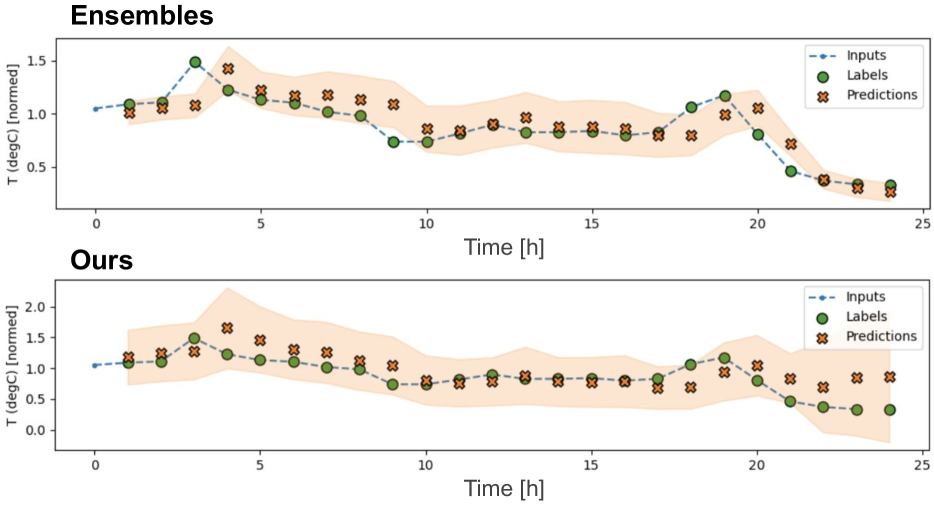
Figure 3: Comparison between Deep Ensembles and our model regarding temperature in Celsius (normalized) for every hour on the same day. More details are in Apd. C.2.

In this setting, we evaluate models in the real world with a weather time series dataset recorded by the Max Planck Institute for Biogeochemistry (Abadi et al., 2015). Specifically, the model will learn to predict the temperature for every hour from 14 different features (collected every 10 minutes), e.g., air temperature, atmospheric pressure, humidity, etc.

Tab. 2 quantitatively shows our method outperforms others in terms of calibration and sharpness in both IID and OOD settings. Notably, its predictive uncertainty is more calibrated and sharper than the well-known SOTA Ensembles. To take a closer look at this difference, we visualize the temperature prediction on OOD data in Fig. 3. We observe that Deep Ensembles is conservative, even when making incorrect predictions. In contrast, our model enables signaling when it is likely wrong. Importantly, it is more calibrated by always covering the true label in our confidence intervals, while at the same time, preserving the sharpness with correct predictions.

4.3 Benchmark UCI

We next conduct another benchmarking experiment on the UCI datasets (Amini et al., 2020). For testing on IID data, we leave tables in Apd. C.3, where our main observation is our Density-Regresiion still performs well in these IID-only dataset by having a low calibration and sharpness value. We mainly discuss the main result under distribution shifts on UCI: Wine Quality, which includes two datasets, related to red and white vinho verde wine samples, from the north of Portugal. The goal is to model wine quality based on physicochemical tests (Cortez et al., 2009). In our setting, we train models on red wine samples, and test on both the IID samples and the white vinho verde wine OOD samples. Tab. 3 shows our Density-Regression outperforms other baselines and has a competitive result with the SOTA Deep Enselbmes in all criteria. Notably, the competitive result is not only in uncertainty quality but also in NLL and RMSE, showing our method is robust under distribution shifts.

4.4 Monocular Depth Estimation

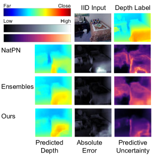
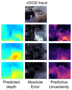
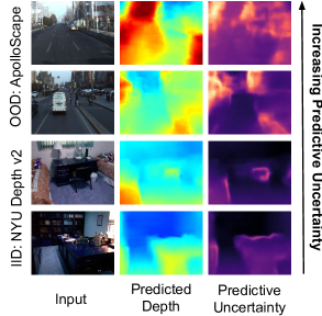
(a)	(b)	(c)

Figure 4: Comparison in pixel-wise depth predictions and predictive uncertainty on (a) IID and (b) $0.04$ noise level on corrupted OOD dataset. Detailed figures for the robustness under corrupted noise are in Apd. C.1; (c) Our model performance on the real-world OOD ApolloScape.

Finally, we present an application of our model in the monocular depth estimation task (Amini et al., 2020). We train models with U-Net (Ronneberger et al., 2015) on $27k$ RGB-to-depth image pairs of indoor scenes (e.g., bedrooms, kitchens, etc.) from the NYU Depth v2 (Silberman et al., 2012). Then, we test on this IID test-set and two OOD datasets, including its corrupted data by adding noise with the Fast Gradient Sign Method (Goodfellow et al., 2015) and a diverse outdoor driving ApolloScape (Huang et al., 2018). Tab. 4 once again confirms Density-Regression consistently provides a good quality uncertainty estimate by always achieving the lowest calibration error across three test sets, especially on the real-world OOD outdoor scenes dataset. Regarding the sharpness, it is worth noticing that, unlike calibration, sharpness is neither a sufficient nor necessary condition for a good uncertainty estimate. It will depend on the model’s accuracy: if a model has a high RMSE (e.g., on OOD outdoor scenes), the sharpness score should be high. Therefore, we marked the bold by comparing the calibration error first, then the sharpness later, i.e., if two models have the same calibration error, we compare their sharpness to select the better one.

To take a closer look at the performance, we visualize Fig. 4 (a) and Fig. 4 (b) to compare the predicted depth map, its error comparing to the ground truth, and the corresponding predicted uncertainty for every pixel. Firstly, we observe that Density-Regression is more robust (i.e., the robustness performance on the OOD data) than NatPN (Charpentier et al., 2022) by lower pixel values in the absolute error image. Secondly, it provides more certain predictions for correct pixels and less certain for incorrect ones than other methods. Finally, it can provide certain predictions on IID data, and when the corrupted OOD images are far from the training set, its certainty decreases correspondingly. This confirms a hypothesis that our model is distance-aware, helping to improve the quality of uncertainty quantification under distribution shifts.

Regarding the real-world OOD ApolloScape, we also observe from Fig. 4 (c) that our model can provide confident prediction on IID images. And when the OOD dataset is far from IID, its predictive uncertainty also increases correspondingly. Additionally, Fig. 5 (c) also shows that when compared to other methods under distribution shifts, our model is also more well-calibrated by less over-confidence and under-confidence, resulting in the closest to the ideal calibration line.

4.5 Test-time Efficiency Evaluation

So far, we have empirically shown our model can provide a high-quality uncertainty estimation and have a competitive result with the SOTA Deep Ensembles across several tasks. We next show that our method outperforms Deep Ensembles regarding test-time efficiency. Indeed, Fig. 5 (a) and Fig. 5 (b) show our model has less than four times the model size and five times faster computation than Ensembles across different GPU architectures. Notably, when compared to the best efficient model, i.e., Deterministic Gaussian DNN, our model is only slightly higher due to $p(Z;\alpha)$ density function (the minus of ours to Deterministic can measure this gap). As a result, our method not only has a better uncertainty quality, but also has a higher test-time efficiency than many sampling-free methods, e.g., Quantile, EDL, NatPN, SNGP, and DUE.

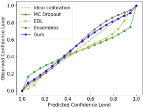
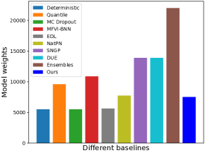
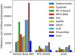
(a)	(b)	(c)

Figure 5: (a) Visualization of calibration error with reliability diagram on the real-world OOD ApolloScape; (b) Comparison in model storage requirement at test-time; (c) Inference cost comparison at test-time across three modern GPU architectures (detailed in Apd. B.2).

5 Related work

Uncertainty and Robustness. More discussion of Uncertainty and Robustness can be found in the literature of  Tran et al. (2022); Bui and Maifeld-Carucci (2022); Ovadia et al. (2019); Koh et al. (2021); Minderer et al. (2021); Hendrycks and Dietterich (2019). For the regression setting, Gustafsson et al. (2023); Tran et al. (2020); Dheur and Ben Taieb (2023) have recently empirically covered SOTA techniques. To summarize, there are three main approaches: sampling-based, sampling-free, and replacing loss function. Regarding sampling-based models, the typical approaches includes GP (Gardner et al., 2018; Lee et al., 2018), BNN (Blundell et al., 2015; Wen et al., 2018), Dropout (Gal and Ghahramani, 2016a, b; Gal et al., 2017), and the SOTA Ensembles (Hansen and Salamon, 1990). These sampling-based models, however, are struggling with scalability in terms of the number of weights and inference speed (Nado et al., 2021). To tackle this challenge, there are some lightweight sampling-based models have been proposed recently, including BatchEnsemble (Wen et al., 2020), Rank-1 BNN (Dusenberry et al., 2020), and Heteroscedastic (Collier et al., 2021). However, these works often only focus on the classification setting.

Therefore, novel sampling-free approaches to improve uncertainty estimation have recently been proposed. Starting with Deterministic Gaussian DNN (Chua et al., 2018), then with Quantile Regression (Koenker and Bassett, 1978; Romano et al., 2019), deterministic GP (Liu et al., 2020; van Amersfoort et al., 2022), and Bayesian inference closed-form based (Amini et al., 2020; Charpentier et al., 2020, 2022). However, the uncertainty quality of these methods is often still degraded when compared to sampling-based models. For instance, if the prior hyper-parameters are poorly defined, the Bayesian-based model EDL (Amini et al., 2020) and Posterior Network (Charpentier et al., 2020) will result in a bad performance in practice. Conversely, Density-Regression does not require any prior hyper-parameters in training and test time. Regarding replacing the loss function, there exists the post-hoc calibration (Kuleshov et al., 2018; Song et al., 2019; Romano et al., 2019; Vovk et al., 2005; Tibshirani et al., 2019; Prinster et al., 2022, 2023) and regularization approaches (Chung et al., 2021; Mukhoti et al., 2020; Dheur and Ben Taieb, 2023). In contrast, our baselines only do MLE using the objective function in Eq. 2 without depending on any regularization or re-calibration set.

Improving uncertainty quality via density estimation. The idea of improving DNN uncertainty via Density Estimation has been significantly studied (Kuleshov and Deshpande, 2022; Charpentier et al., 2022, 2020; Mukhoti et al., 2023; Kotelevskii et al., 2022). However, these work either entail post-hoc re-calibration, OOD samples in training, or pre-defined prior parameters in test time. For instance, NatPN (Charpentier et al., 2022, 2020) customizes the last layer of DNN with sensitive priors, not normalized by a natural exponent function, resulting in a bad accuracy performance in practice (Nado et al., 2021).

To summarize, compared to prior work, our method does not use any post-hoc re-calibration, OOD samples in training, or pre-defined prior parameters in test time. Closest to our work is Density-Softmax (Bui and Liu, 2024), which is also based on density function and distance awareness property to enhance the quality of uncertainty estimation and robustness under distribution shifts. However, it only works for the classification task, and extending to the regression task is non-trivial.

6 Conclusion

Improving uncertainty quantification is a critical problem in trustworthy AI. There has been growing interested in using sampling-based methods to ensure AI systems are reliable. Challenges often arise when deploying such models in real-world domains. In this regard, our Density-Regression significantly improves test-time efficiency while preserving reliability. We provide theoretical guarantees for our framework and prove it is distance-aware on the feature space. With this property, we empirically show our method is fast, lightweight, and provides high-quality uncertainty estimates in plenty of high-stake real-world applications like weather forecasting and depth estimation. Given this, we hope Density-Regression will inspire researchers and developers to make further progress in improving the efficiency and trustworthiness of DNN.

Checklist

1. For all models and algorithms presented, check if you include:

   1. A clear description of the mathematical setting, assumptions, algorithm, and/or model. [Yes]

   2. An analysis of the properties and complexity (time, space, sample size) of any algorithm. [Yes]

   3. (Optional) Anonymized source code, with specification of all dependencies, including external libraries. [Yes]

2. For any theoretical claim, check if you include:

   1. Statements of the full set of assumptions of all theoretical results. [Not Applicable]

   2. Complete proofs of all theoretical results. [Yes]

   3. Clear explanations of any assumptions. [Not Applicable]

3. For all figures and tables that present empirical results, check if you include:

   1. The code, data, and instructions needed to reproduce the main experimental results (either in the supplemental material or as a URL). [Yes]

   2. All the training details (e.g., data splits, hyperparameters, how they were chosen). [Yes]

   3. A clear definition of the specific measure or statistics and error bars (e.g., with respect to the random seed after running experiments multiple times). [Yes]

   4. A description of the computing infrastructure used. (e.g., type of GPUs, internal cluster, or cloud provider). [Yes]

4. If you are using existing assets (e.g., code, data, models) or curating/releasing new assets, check if you include:

   1. Citations of the creator If your work uses existing assets. [Yes]

   2. The license information of the assets, if applicable. [Not Applicable]

   3. New assets either in the supplemental material or as a URL, if applicable. [Not Applicable]

   4. Information about consent from data providers/curators. [Not Applicable]

   5. Discussion of sensible content if applicable, e.g., personally identifiable information or offensive content. [Not Applicable]

5. If you used crowdsourcing or conducted research with human subjects, check if you include:

   1. The full text of instructions given to participants and screenshots. [Not Applicable]

   2. Descriptions of potential participant risks, with links to Institutional Review Board (IRB) approvals if applicable. [Not Applicable]

   3. The estimated hourly wage paid to participants and the total amount spent on participant compensation. [Not Applicable]

 

Density-Regression: Efficient and Distance-Aware Deep Regressor for Uncertainty Estimation under Distribution Shifts
(Supplementary Material)

  Broader impacts. High-quality uncertainty estimate is an important property in trustworthy AI, and Density-Regression can significantly improve uncertainty quality and test-time efficiency. This could be particularly beneficial in high-stake applications (e.g., healthcare, finance, policy decision-making, etc.), where the trained model needs to be deployed and inference on low-resource hardware or real-time response software.

Limitations:

1. Density model performance in practice. The uncertainty quality of Density-Regression depends on the density function. Our results show if the likelihood on test OOD feature is lower than IID set, then Density-Regression can reduce the over-confidence of Deterministic Gaussian DNN. That said, it can be a risk that our model might not fully capture the real-world complexity by estimating density function is not always trivial in practice (Nalisnick et al., 2019; Bui and Liu, 2024; Charpentier et al., 2022).

2. Training cost. Despite showing success in test-time efficiency, we raise awareness about the challenge of training Density-Regression. Specifically, Density-Regression requires a longer training time than Deterministic Gaussian DNN due to three separate training steps in Alg. 1 (e.g., Fig. 14).

Remediation. Given the aforementioned limitations, we encourage people who extend our work to: (1) proactively confront the model design and parameters to desired behaviors in real-world use cases; (2) be aware of the training challenge and prepare enough time to pre-train our framework in practice.

Future work. We plan to tackle Density-Regression’s limitations, including improving estimation techniques to enhance the quality of the density function and continuing to reduce the number of parameters to deploy this framework in real-world systems.

Reproducibility. The source code to reproduce our results is in the attached zip file of this supplementary material. We provide all proofs in Apd. A, experimental settings in Apd. B, and detailed results in Apd. C.

Appendix A Proofs

In this appendix, we provide the proofs for all the results in the main paper.

A.1 Lemma A.1 and the proof

Lemma A.1.

When $\mathcal{Y}$ is the label space and $\Phi(x,y)$ is the sufficient statistic of the joint distribution $\mathbb{P}(x,y)$ associated with $(x,y)\in\mathcal{X}\times\mathcal{Y}$, we have the predictive distribution follows

$$p(y|x;\theta)=\exp\left(\eta(\theta_{g})^{\top}\Phi(f(x),y)-\log\left(\int_{y^{\prime}\in\mathcal{Y}}\exp\left(\eta(\theta_{g})^{\top}\Phi(f(x),y^{\prime})\right)dy^{\prime}\right)\right),$$ (16)

where $\theta=(\theta_{g},\theta_{f})$ is the parameter vector of the forecast $h=g\circ f$ and $\eta$ is the natural function for the parameter $\theta$.

Proof.

We have a random variable $x$ that belongs to the exponential family with the Probability density function

$$p(x;\theta)=h(x)\exp(\eta(\theta)^{\top}\Phi(x)-A(\theta)),$$ (17)

where $h(x)$ is the underlying measure, $\theta$ is the parameter vector, $\eta$ is the natural function for parameter $\theta$, $\Phi(x)$ is the sufficient statistic, and the log-normalizer

$$A(\theta)=\log\int_{\mathcal{X}}h(x)\exp\left(\eta(\theta)^{\top}\Phi(x)\right)dx.$$ (18)

For $\mathcal{Y}$ is the label space and $\Phi(x,y)$ is the sufficient statistic of the joint distribution $\mathbb{P}(x,y)$ associated with $(x,y)\in\mathcal{X}\times\mathcal{Y}$, we have the join Probability density function

$$p(x,y;\theta)=h(x)\exp\left(\eta(\theta)^{\top}\Phi(x,y)-A(\theta)\right).$$ (19)

By Bayes’s rule, we obtain

$$p(y|x;\theta)=\frac{p(x|y;\theta)}{\int_{y^{\prime}\in\mathcal{Y}}p(x|y^{\prime};\theta)p(y^{\prime}|\theta)dy^{\prime}}=\frac{p(x,y;\theta)}{\int_{y^{\prime}\in\mathcal{Y}}p(x,y^{\prime};\theta)dy^{\prime}}=\frac{h(x)\exp\left(\eta(\theta)^{\top}\Phi(x,y)-A(\theta)\right)}{\int_{y^{\prime}\in\mathcal{Y}}h(x)\exp\left(\eta(\theta)^{\top}\Phi(x,y^{\prime})-A(\theta)\right)dy^{\prime}}.$$ (20)

Assumed the $h(x)$ base reference measure to be a function only of $x$ so that we can cancel it from the numerator and denominator in the last step above. Therefore, we get

$$p(y|x;\theta)=\frac{\exp\left(\eta(\theta)^{\top}\Phi(x,y)\right)}{\int_{y^{\prime}\in\mathcal{Y}}\exp\left(\eta(\theta)^{\top}\Phi(x,y^{\prime})\right)dy^{\prime}}=\exp\left(\eta(\theta)^{\top}\Phi(x,y)-\log\left(\int_{y^{\prime}\in\mathcal{Y}}\exp\left(\eta(\theta)^{\top}\Phi(x,y^{\prime})\right)dy^{\prime}\right)\right).$$ (21)

As a result, when $y=g(f(x))$, we obtain

$$p(y|x;\theta) =\exp\left(\eta(\theta_{g})^{\top}\Phi(f(x),y)-\log\left(\int_{y^{\prime}\in\mathcal{Y}}\exp\left(\eta(\theta_{g})^{\top}\Phi(f(x),y^{\prime})\right)dy^{\prime}\right)\right)$$ (22)

$$=\frac{\exp\left(\eta(\theta_{g})^{\top}\Phi(f(x),y)\right)}{\int_{y^{\prime}\in\mathcal{Y}}\exp\left(\eta(\theta_{g})^{\top}\Phi(f(x),y^{\prime})\right)dy^{\prime}}$$ (23)

of Lemma A.1 ∎

A.2 Proof of Theorem 3.1

Proof.

Since the sufficient statistic has the form $\Phi(z,y)=\begin{bmatrix}zy^{2}&y^{2}&2zy&2y&z&1\end{bmatrix}$, where $z=f(x)$, replace it to the dot product of the natural parameter $\eta(\theta)$ with sufficient statistic $\Phi(z,y)$, we get

$$\eta(\theta_{g})^{\top}\Phi(z,y) =\begin{bmatrix}\theta_{1}&\theta_{2}&\theta_{3}&\theta_{4}&\theta_{5}&\theta_{6}\end{bmatrix}\begin{bmatrix}zy^{2}&y^{2}&2zy&2y&z&1\end{bmatrix}^{\top}$$ (24)

$$=\begin{bmatrix}\theta_{1}&\theta_{2}\end{bmatrix}\begin{bmatrix}z\\ 1\end{bmatrix}y^{2}+2\begin{bmatrix}\theta_{3}&\theta_{4}\end{bmatrix}\begin{bmatrix}z\\ 1\end{bmatrix}y+\begin{bmatrix}\theta_{5}&\theta_{6}\end{bmatrix}\begin{bmatrix}z\\ 1\end{bmatrix}$$ (25)

$$=\begin{bmatrix}\theta_{1}&\theta_{2}\end{bmatrix}\begin{bmatrix}z\\ 1\end{bmatrix}y^{2}+2\begin{bmatrix}\theta_{3}&\theta_{4}\end{bmatrix}\begin{bmatrix}z\\ 1\end{bmatrix}y+\frac{\left(-\begin{bmatrix}\theta_{3}&\theta_{4}\end{bmatrix}\begin{bmatrix}z\\ 1\end{bmatrix}\right)^{2}}{\begin{bmatrix}\theta_{1}&\theta_{2}\end{bmatrix}\begin{bmatrix}z\\ 1\end{bmatrix}}$$ (26)

$$=\theta_{g}^{\sigma}\begin{bmatrix}z\\ 1\end{bmatrix}y^{2}+2\theta_{(y,x_{1})}\begin{bmatrix}z\\ 1\end{bmatrix}y+\frac{\left(-\theta_{g}^{\mu}\begin{bmatrix}z\\ 1\end{bmatrix}\right)^{2}}{\theta_{g}^{\sigma}\begin{bmatrix}z\\ 1\end{bmatrix}}.$$ (27)

Hence, we get

$$-p(z;\alpha)\eta(\theta_{g})^{\top}\Phi(z,y)=-p(z;\alpha)\theta_{g}^{\sigma}\begin{bmatrix}z\\ 1\end{bmatrix}y^{2}-2p(z;\alpha)\theta_{g}^{\mu}\begin{bmatrix}z\\ 1\end{bmatrix}y-p(z;\alpha)\frac{\left(-\theta_{g}^{\mu}\begin{bmatrix}z\\ 1\end{bmatrix}\right)^{2}}{\theta_{g}^{\sigma}\begin{bmatrix}z\\ 1\end{bmatrix}},$$ (28)

and the corresponding log-normalizer

$$\log\int_{\mathcal{Y}}\exp\left(-p(z;\alpha)\eta(\theta_{g})^{\top}\Phi(z,y)\right)dy$$ (29)

$$=\log\int_{\mathcal{Y}}\exp\left(-p(z;\alpha)\theta_{g}^{\sigma}\begin{bmatrix}z\\ 1\end{bmatrix}y^{2}-2p(z;\alpha)\theta_{g}^{\mu}\begin{bmatrix}z\\ 1\end{bmatrix}y-p(z;\alpha)\frac{\left(-\theta_{g}^{\mu}\begin{bmatrix}z\\ 1\end{bmatrix}\right)^{2}}{\theta_{g}^{\sigma}\begin{bmatrix}z\\ 1\end{bmatrix}}\right)dy$$ (30)

$$=\log\left(\sqrt{\frac{\pi}{p(z;\alpha)\theta_{g}^{\sigma}\begin{bmatrix}z\\ 1\end{bmatrix}}}\exp\left(\underbrace{\frac{\left(2p(z;\alpha)\theta_{g}^{\mu}\begin{bmatrix}z\\ 1\end{bmatrix}\right)^{2}}{4p(z;\alpha)\theta_{g}^{\sigma}\begin{bmatrix}z\\ 1\end{bmatrix}}-p(z;\alpha)\frac{\left(-\theta_{g}^{\mu}\begin{bmatrix}z\\ 1\end{bmatrix}\right)^{2}}{\theta_{g}^{\sigma}\begin{bmatrix}z\\ 1\end{bmatrix}}}_{0}\right)\right)$$ (31)

$$=\log\left(\sqrt{\frac{\pi}{p(z;\alpha)\theta_{g}^{\sigma}\begin{bmatrix}z\\ 1\end{bmatrix}}}\right)=\frac{1}{2}\log\left(\frac{\pi}{p(z;\alpha)\theta_{g}^{\sigma}\begin{bmatrix}z\\ 1\end{bmatrix}}\right).$$ (32)

So, replace the result of Equation 28 and Equation 29 to the Exponential form of Density-Regressor, we obtain

$$p(y|x;\theta)=\exp\left(-p(z;\alpha)\eta(\theta_{g})^{\top}\Phi(z,y)-\log\int_{\mathcal{Y}}\exp\left(-p(z;\alpha)\eta(\theta_{g})^{\top}\Phi(z,y)\right)dy\right)\text{, where }z=f(x)$$ (33)

$$=\exp\left(-p(z;\alpha)\theta_{g}^{\sigma}\begin{bmatrix}z\\ 1\end{bmatrix}y^{2}-2p(z;\alpha)\theta_{g}^{\mu}\begin{bmatrix}z\\ 1\end{bmatrix}y-p(z;\alpha)\frac{\left(-\theta_{g}^{\mu}\begin{bmatrix}z\\ 1\end{bmatrix}\right)^{2}}{\theta_{g}^{\sigma}\begin{bmatrix}z\\ 1\end{bmatrix}}-\frac{1}{2}\log\left(\frac{\pi}{p(z;\alpha)\theta_{g}^{\sigma}\begin{bmatrix}z\\ 1\end{bmatrix}}\right)\right)$$ (34)

$$=\exp\{\frac{-1}{2}2\cdot p(z;\alpha)\theta_{g}^{\sigma}\begin{bmatrix}z\\ 1\end{bmatrix}y^{2}+2\cdot p(z;\alpha)\theta_{g}^{\sigma}\begin{bmatrix}z\\ 1\end{bmatrix}\frac{-\theta_{g}^{\mu}\begin{bmatrix}z\\ 1\end{bmatrix}}{\theta_{g}^{\sigma}\begin{bmatrix}z\\ 1\end{bmatrix}}y$$ (35)

$$-\left(\frac{-\theta_{g}^{\mu}\begin{bmatrix}z\\ 1\end{bmatrix}}{\theta_{g}^{\sigma}\begin{bmatrix}z\\ 1\end{bmatrix}}\right)^{2}\left(\frac{1}{2}2\cdot p(z;\alpha)\theta_{g}^{\sigma}\begin{bmatrix}z\\ 1\end{bmatrix}\right)-\frac{1}{2}\log\left(2\pi\frac{1}{2\cdot p(z;\alpha)\theta_{g}^{\sigma}\begin{bmatrix}z\\ 1\end{bmatrix}}\right)\}.$$ (36)

On the other hand, we have the Probability density function of the Gaussian distribution $\mathcal{N}(\mu,\sigma^{2})$ has the form

$$p(y|x;\theta) =\exp\left(\frac{-1}{2\sigma^{2}}y^{2}+\frac{\mu}{\sigma^{2}}y-\frac{1}{2\sigma^{2}}\mu^{2}-\frac{1}{2}\log(2\pi\sigma^{2})\right)$$ (37)

$$=\exp\left(\frac{-1}{2\sigma^{2}}y^{2}+\frac{\mu}{\sigma^{2}}y-\left(\frac{1}{2\sigma^{2}}\mu^{2}+\frac{1}{2}\log(2\pi\sigma^{2})\right)\right).$$ (38)

Applying the result from Lemma A.1, when the Exponential family has the form

$$p(y|x;\theta)=\exp\left(\eta(\theta_{g})^{\top}\Phi(z=f(x),y)-\log\int_{\mathcal{Y}}\exp\left(\eta(\theta_{g})^{\top}\Phi(z=f(x),y)\right)dy\right),$$ (39)

we obtain

$$\log\int_{\mathcal{Y}}\exp\left(\frac{-1}{2\sigma^{2}}y^{2}+\frac{\mu}{\sigma^{2}}y\right)dy=\log\left(\sqrt{\pi 2\sigma^{2}}\exp\left(\frac{\mu^{2}}{\sigma^{4}}\frac{2\sigma^{2}}{4}\right)\right)=\frac{1}{2\sigma^{2}}\mu^{2}+\frac{1}{2}\log(2\pi\sigma^{2}).$$ (40)

Combining the result from Equation 33, Equation 37, and Equation 40, we get

$$p(y|x;\theta) =\exp\{\frac{-1}{2}\underbrace{2\cdot p(z;\alpha)\theta_{g}^{\sigma}\begin{bmatrix}z\\ 1\end{bmatrix}}_{\sigma^{2}(x,\theta)^{-1}}y^{2}+\underbrace{2\cdot p(z;\alpha)\theta_{g}^{\sigma}\begin{bmatrix}z\\ 1\end{bmatrix}}_{\sigma^{2}(x,\theta)^{-1}}\underbrace{\frac{-\theta_{g}^{\mu}\begin{bmatrix}z\\ 1\end{bmatrix}}{\theta_{g}^{\sigma}\begin{bmatrix}z\\ 1\end{bmatrix}}}_{\mu(x,\theta)}y$$ (41)

$$-\left(\underbrace{\left(\frac{-\theta_{g}^{\mu}\begin{bmatrix}z\\ 1\end{bmatrix}}{\theta_{g}^{\sigma}\begin{bmatrix}z\\ 1\end{bmatrix}}\right)^{2}}_{\mu(x,\theta)^{2}}\underbrace{\left(\frac{1}{2}2\cdot p(z;\alpha)\theta_{g}^{\sigma}\begin{bmatrix}z\\ 1\end{bmatrix}\right)}_{\left(2\sigma^{2}(x.\theta)\right)^{-1}}+\frac{1}{2}\log\left(2\pi\underbrace{\frac{1}{2\cdot p(z;\alpha)\theta_{g}^{\sigma}\begin{bmatrix}z\\ 1\end{bmatrix}}}_{\sigma^{2}(x,\theta)}\right)\right)\}.$$ (42)

As a result, we obtain $p(y|x;\theta)\sim\mathcal{N}(\mu(x,\theta),\sigma^{2}(x,\theta))$, where

$$\mu(x,\theta)=-\left(\theta_{g}^{\sigma}\begin{bmatrix}z\\ 1\end{bmatrix}\right)^{-1}\left(\theta_{g}^{\mu}{\begin{bmatrix}z\\ 1\end{bmatrix}}\right)\text{ and }\sigma^{2}(x,\theta)=\left(2\cdot p(z;\alpha)\theta_{g}^{\sigma}\begin{bmatrix}z\\ 1\end{bmatrix}\right)^{-1}$$ (43)

of Theorem 3.1. ∎

A.3 Proof of Corollary 3.2

Proof.

From the result of Theorem 3.1, we have

$$\mu(x,\theta)=-\left(\theta_{g}^{\sigma}\begin{bmatrix}z\\ 1\end{bmatrix}\right)^{-1}\left(\theta_{g}^{\mu}{\begin{bmatrix}z\\ 1\end{bmatrix}}\right)\text{ and }\sigma^{2}(x,\theta)=\left(2\cdot p(z;\alpha)\theta_{g}^{\sigma}\begin{bmatrix}z\\ 1\end{bmatrix}\right)^{-1}.$$ (44)

Hence, firstly, we can rewrite the mean by

$$\mu(x,\theta)=\underbrace{\left(2\cdot p(z;\alpha)\theta_{g}^{\sigma}\begin{bmatrix}z\\ 1\end{bmatrix}\right)^{-1}}_{\sigma^{2}(z,\theta)}-2\cdot p(z;\alpha)\theta_{g}^{\mu}{\begin{bmatrix}z\\ 1\end{bmatrix}}.$$ (45)

On the other hand, we have the log of standard deviation as follows

$$\log(\sigma(x,\theta)) =\log\left(\frac{1}{\sqrt{2\cdot p(z;\alpha)\theta_{g}^{\sigma}\begin{bmatrix}z\\ 1\end{bmatrix}}}\right)=-\log\left(2\cdot p(z;\alpha)\theta_{g}^{\sigma}\begin{bmatrix}z\\ 1\end{bmatrix}\right)^{\frac{1}{2}}$$ (46)

$$=-\frac{1}{2}\log\left(2\cdot p(z;\alpha)\theta_{g}^{\sigma}\begin{bmatrix}z\\ 1\end{bmatrix}\right)=-\frac{1}{2}\left[\log(2)+\log(p(z;\alpha))+\log(\theta_{g}^{\sigma}\begin{bmatrix}z\\ 1\end{bmatrix})\right]$$ (47)

$$=-\frac{1}{2}\left[\log(2)+\log(p(z;\alpha))+\theta_{g}^{\sigma}\begin{bmatrix}z\\ 1\end{bmatrix}\right]\text{ (parameterised directly the $\log$ by $\theta_{g}^{\sigma}\begin{bmatrix}z\\ 1\end{bmatrix}$)}.$$ (48)

Therefore, we obtain the variance

$$\sigma^{2}(x;\theta)=\exp\left(\log(\sigma(x,\theta))\right)^{2}=\exp\left(-\frac{1}{2}\left[\log(2)+\log(p(z;\alpha))+\theta_{g}^{\sigma}\begin{bmatrix}z\\ 1\end{bmatrix}\right]\right)^{2}$$ (49)

of Corollary 3.2. ∎

A.4 Proof of Theorem 3.5

Proof.

Using Lemma 3.4, we have $\lim_{d(z_{t},Z_{s})\rightarrow\infty}p(z_{t};\alpha)\rightarrow 0$, i.e., if $d(z_{ood},Z_{s})\rightarrow\infty$ then $p(z_{ood};\alpha)\rightarrow 0$. Therefore, we obtain

$$\lim_{p(z_{ood};\alpha)\rightarrow 0}\sigma^{2}(x_{ood};\theta)=\lim_{p(z_{ood};\alpha)\rightarrow 0}\left(2\cdot p(z_{ood};\alpha)\theta_{g}^{\sigma}\begin{bmatrix}z\\ 1\end{bmatrix}\right)^{-1}=\infty.$$ (50)

Conversely, we have $\lim_{d(z_{t},Z_{s})\rightarrow 0}p(z_{t};\alpha)\rightarrow\infty$, i.e., if $d(z_{iid},Z_{s})\rightarrow 0$ then $p(z_{iid};\alpha)\rightarrow\infty$. Therefore, we obtain

$$\lim_{p(z_{iid};\alpha)\rightarrow\infty}\sigma^{2}(x_{iid};\theta)=\lim_{p(z_{iid};\alpha)\rightarrow\infty}\left(2\cdot p(z_{iid};\alpha)\theta_{g}^{\sigma}\begin{bmatrix}z\\ 1\end{bmatrix}\right)^{-1}=0$$ (51)

of Theorem 3.5. ∎

A.5 Proof of Theorem 3.6

Proof.

The proofs contain three parts. The first part shows density function $p(z_{t};\alpha)$ is monotonically decreasing w.r.t. distance function $\mathbb{E}\left\|z_{t}-Z_{s}\right\|_{\mathcal{Z}}$. The second part shows the metric $u(x_{t})$ is maximized when $p(z_{t};\alpha)\rightarrow 0$. The third part shows $u(x_{t})$ monotonically decreasing w.r.t. $p(z_{t};\alpha)$ on the interval $\left(0,\infty\right]$.

Part (1). The monotonic decrease of density function $p(z_{t};\alpha)$ w.r.t. distance function $\mathbb{E}\left\|z_{t}-Z_{s}\right\|_{\mathcal{Z}}$: Consider the probability density function $p(z_{t};\alpha)$ follows Normalizing-Flows which output the Gaussian distribution with mean (median) $\mu$ and standard deviation $\sigma$, then we have

$$p(z_{t};\alpha)=\frac{1}{\sigma\sqrt{2\pi}}\exp\left(\frac{-1}{2}\left(\frac{z_{t}-\mu}{\sigma}\right)^{2}\right).$$ (52)

Take derivative, we obtain

$$\frac{d}{dz_{t}}p(z_{t};\alpha) =\left[\frac{-1}{2}\left(\frac{z_{t}-\mu}{\sigma}\right)^{2}\right]^{\prime}p(z_{t};\alpha)=\frac{\mu-z_{t}}{\sigma^{2}}p(z_{t};\alpha)\Rightarrow\begin{cases}\frac{d}{dz_{t}}p(z_{t};\alpha)>0&\text{ if }z_{t}<\mu,\\ \\ \frac{d}{dz_{t}}p(z_{t};\alpha)=0&\text{ if }z_{t}=\mu,\\ \\ \frac{d}{dz_{t}}p(z_{t};\alpha)<0&\text{ if }z_{t}>\mu.\end{cases}$$ (53)

Consider the distance function $\mathbb{E}\left\|z_{t}-Z_{s}\right\|_{\mathcal{Z}}$ follows the absolute norm, then we have

$$\mathbb{E}\left\|z_{t}-Z_{s}\right\|_{\mathcal{Z}}=\mathbb{E}\left(\left|z_{t}-Z_{s}\right|\right)=\int_{-\infty}^{z_{t}}\mathbb{P}(Z_{s}\leq t)dt+\int_{z_{t}}^{+\infty}\mathbb{P}(Z_{s}\geq t)dt.$$ (54)

Take derivative, we obtain

$$\frac{d}{dz_{t}}\mathbb{E}\left\|z_{t}-Z_{s}\right\|_{\mathcal{Z}}=\mathbb{P}(Z_{s}\leq z_{t})-\mathbb{P}(Z_{s}\geq z_{t})\Rightarrow\begin{cases}\frac{d}{dz_{t}}\mathbb{E}\left\|z_{t}-Z_{s}\right\|_{\mathcal{Z}}<0&\text{ if }z_{t}<\mu,\\ \\ \frac{d}{dz_{t}}\mathbb{E}\left\|z_{t}-Z_{s}\right\|_{\mathcal{Z}}=0&\text{ if }z_{t}=\mu,\\ \\ \frac{d}{dz_{t}}\mathbb{E}\left\|z_{t}-Z_{s}\right\|_{\mathcal{Z}}>0&\text{ if }z_{t}>\mu.\end{cases}$$ (55)

Combining the result in Equation 53 and Equation 55, we have $p(z_{t};\alpha)$ is maximized when $\mathbb{E}\left\|z_{t}-Z_{s}\right\|_{\mathcal{Z}}$ is minimized at the median $\mu$, $p(z_{t};\alpha)$ increase when $\mathbb{E}\left\|z_{t}-Z_{s}\right\|_{\mathcal{Z}}$ decrease and vice versa. As a consequence, we obtain $p(z_{t};\alpha)$ is monotonically decreasing w.r.t. distance function $\mathbb{E}\left\|z_{t}-Z_{s}\right\|_{\mathcal{Z}}$.

Part (2). The maximum of metric $u(x_{t})$: Consider $u(x_{t})=v(d(x_{t},X_{s}))$ in Def. 2.2, let $u(x_{t})$ is the entropy of predictive distribution of Density-Regression $p(y|x;\theta)$, i.e., $u(x_{t})=\mathrm{H}(Y|X=x_{t})$, where $\mathrm{H}(Y|X=x_{t})$ be the entropy of $Y$ conditioned on $X$ taking a certain value $x_{t}$ via $p(y|x;\theta)$. When the predictive distribution of Density-Regression follows the Normal distribution, i.e., $p(y|x;\theta)\sim\mathcal{N}(\mu(x,\theta),\sigma^{2}(x,\theta))$, we have

$$u(x_{t}) =\mathrm{H}(Y|X=x_{t})=-\int_{\mathcal{Y}}p(y|x_{t})\log(p(y|x_{t}))dy$$ (56)

$$=-\int_{\mathcal{Y}}\frac{1}{\sqrt{2\pi\sigma^{2}(x_{t},\theta)}}\exp\left(-\frac{\left(y-\mu(x_{t},\theta)^{2}\right)}{2\sigma^{2}(x_{t},\theta)}\right)\log\left[\frac{1}{\sqrt{2\pi\sigma^{2}(x_{t},\theta)}}\exp\left(-\frac{\left(y-\mu(x_{t},\theta)^{2}\right)}{2\sigma^{2}(x_{t},\theta)}\right)\right]dy$$ (57)

$$=-\int_{\mathcal{Y}}\frac{1}{\sqrt{2\pi\sigma^{2}(x_{t},\theta)}}\exp\left(-\frac{\left(y-\mu(x_{t},\theta)^{2}\right)}{2\sigma^{2}(x_{t},\theta)}\right)\left[\log\left(\frac{1}{\sqrt{2\pi\sigma^{2}(x_{t},\theta)}}\right)-\left(\frac{\left(y-\mu(x_{t},\theta)^{2}\right)}{2\sigma^{2}(x_{t},\theta)}\right)\right]dy$$ (58)

$$=-\log\left(\frac{1}{\sqrt{2\pi\sigma^{2}(x_{t},\theta)}}\right)\underbrace{\int_{\mathcal{Y}}\underbrace{\frac{\exp\left(-\frac{\left(y-\mu(x_{t},\theta)^{2}\right)}{2\sigma^{2}(x_{t},\theta)}\right)}{\sqrt{2\pi\sigma^{2}(x_{t},\theta)}}}_{p(y|x_{t})}dy}_{1}+\int_{\mathcal{Y}}\left(\frac{\left(y-\mu(x_{t},\theta)^{2}\right)}{2\sigma^{2}(x_{t},\theta)}\right)\underbrace{\frac{\exp\left(-\frac{\left(y-\mu(x_{t},\theta)^{2}\right)}{2\sigma^{2}(x_{t},\theta)}\right)}{\sqrt{2\pi\sigma^{2}(x_{t},\theta)}}}_{p(y|x_{t})}dy$$ (59)

$$=\frac{1}{2}\log\left(2\pi\sigma^{2}(x_{t},\theta)\right)+\frac{1}{2\sigma^{2}(x_{t},\theta)}\int_{\mathcal{Y}}\left(y-\mu(x_{t},\theta)\right)^{2}dy.$$ (60)

Combine with the fact that $\int_{\mathcal{Y}}\left(y-\mu(x_{t},\theta)\right)^{2}dy=\sigma^{2}(x_{t},\theta)$, we obtain

$$u(x_{t})=\frac{1}{2}\log\left(2\pi\sigma^{2}(x_{t},\theta)\right)+\frac{1}{2}.$$ (61)

Since $u(x_{t})$ is now just a continuous function of its variance $\sigma^{2}(x_{t},\theta)$, it is monotone increasing w.r.t. $\sigma^{2}(x_{t},\theta)$ on the interval $(0,\infty]$. Therefore, we get $u(x_{t})$ is maximized when $\sigma^{2}(x_{t};\theta)$ is maximized. As a result, when $\sigma^{2}(x_{t},\theta)=\left(2\cdot p(z_{t};\alpha)\theta_{g}^{\sigma}\begin{bmatrix}z_{t}\\ 1\end{bmatrix}\right)^{-1}$, where $z_{t}=f(x_{t})$, we obtain $u(x_{t})$ is maximized when $p(z_{t};\alpha)\rightarrow 0$, which will happen if $z_{t}$ is OOD data (by the result in Thm. 3.5 and Proof A.4).

Part (3). The monotonically decrease of metric $u(x_{t})$ on the interval $\left(0,\infty\right]$: Consider the function

$$\mathcal{F}(p(z_{t};\alpha))=\frac{1}{2}\log\left(2\pi\left(2\cdot p(z_{t};\alpha)\theta_{g}^{\sigma}\begin{bmatrix}z_{t}\\ 1\end{bmatrix}\right)^{-1}\right)+\frac{1}{2}.$$ (62)

Let $a=p(z_{t};\alpha)$, $b=\theta_{g}^{\sigma}\begin{bmatrix}z_{t}\\ 1\end{bmatrix}$, then

$$\mathcal{F}(a)=\frac{1}{2}\log\left(\frac{2\pi}{2ab}\right)+\frac{1}{2}=\frac{1}{2}\left[\log(\pi)-\log(ab)\right]+\frac{1}{2},$$ (63)

and we need to find $\frac{d}{da}\mathcal{F}$. Take derivative, we obtain

$$\frac{d}{da}\mathcal{F}=\frac{-1}{2a}<0\text{ (due to $a\in\left(0,\infty\right]$)},$$ (64)

combining with $u(x_{t})$ is maximized if $a\rightarrow 0$, we obtain $u(x_{t})$ decrease monotonically on the interval $\left(0,\infty\right]$.

Combining the result in Part (2). $u(x_{t})$ is maximized if $p(z_{t};\alpha)\rightarrow 0$ which will happen if $z_{t}$ is OOD data, and the result in Part (3). $u(x_{t})$ is decrease monotonically w.r.t. $p(z_{t};\alpha)$ on the interval $\left(0,\infty\right]$, which will happen if $x_{t}$ is closer to IID data since the likelihood value $p(z_{t};\alpha)$ increases, we obtain the distance awareness of $-p(z;\alpha)\theta_{g}^{\top}\Phi(z,y)$.

Combining the result in Part (1). $p(z_{t};\alpha)$ is monotonically decreasing w.r.t. distance function $\mathbb{E}\left\|z_{t}-Z_{s}\right\|_{\mathcal{Z}}$ and the result distance awareness of $-p(z;\alpha)\theta_{g}^{\top}\Phi(z,y)$, we obtain the conclusion: $p(y|x;\theta)\propto\exp(-p(f(x);\alpha)\theta_{g}^{\top}\Phi(f(x),y))$ is distance aware on feature space $\mathcal{Z}$ of Theorem 3.6. ∎

Appendix B Experimental settings

In this appendix, we summarize the baselines that we compared in our experiments and provide more detail about our implementation as well as the demo code snippet.

B.1 Baseline details

We provide an exhaustive literature review of 10 SOTA related methods which are used to make comparisons with our model:

• Deterministic DNN (Vapnik, 1998) corresponds to Deterministic Regression in Section 2.

• Deterministic Gaussian DNN (Chua et al., 2018) is discussed in Section 2.

• Quantile Regression (Romano et al., 2019) makes the forecast $h:\mathcal{X}\rightarrow\mathbb{R}^{2}$ to output the prediction intervals with the lower quantile $q^{\alpha/2}(x)=\inf\{y\in\mathbb{R}:F_{Y|X}(y|x)>\alpha/2\}$ and upper quantile $q^{1-\alpha/2}(x)=\inf\{y\in\mathbb{R}:F_{Y|X}(y|x)>(1-\alpha/2)\}$, where $F_{Y|X}$ is the conditional CDF. Then, this forecast $h$ will be trained by using the pinball loss (Steinwart and Christmann, 2011).

• MC Dropout (Gal and Ghahramani, 2016a) includes dropout regularization method in the model. In test-time, it uses MC sampling by dropout to make different predictions, then obtain the final mean and variance by Equation. 3.

• MFVI BNN (Wen et al., 2018) uses the BNN by putting distribution over the weight by mean and variance per each weight. In test-time, it performs prediction by using Equation. 3. Because each weight consists of mean and variance, the total model weights will double as the Deterministic DNN.

• EDL (Amini et al., 2020) is based on Evidential Deep Learning (Sensoy et al., 2018) by making use of conjugate prior property in Bayesian Inference to compute posterior distribution in closed-form. This approach is sensitive to hyper-parameters by requiring to selection of Prior’s parameters.

• NatPN (Charpentier et al., 2022) is the closest to our work by also estimating the density function on the marginal feature space. However, it is based on EDL so their loss function and the regressor function are different by the Bayesian approach. Due to belonging to the Bayesian perspective like EDL, it needs to select a "good" Prior distribution, which is often difficult in practice.

• SNGP (Liu et al., 2020) is a combination of the last GP layer with Spectral Normalization to the hidden layers. This algorithm is primarily designed for the classification, however, we can extend it to the regression task by making the GP layer output the mean and variance like Deterministic Gaussian DNN.

• DUE (van Amersfoort et al., 2022) is an extension version of SNGP by constrain Deep Kernel Learning’s feature extractor to approximately preserve distances through a bi-Lipschitz constraint.

• Deep Ensembles (Lakshminarayanan et al., 2017) includes multiple Deterministic DNN trained with different seeds. In test-time, the final prediction is calculated from the mean of the list prediction of the ensemble by Equation. 3. Due to aggregates from multiple deterministic models, the latency and total of model weights needed to store will increase linearly w.r.t. the number of models.

B.2 Implementation

Dataset, source code, and hyper-parameter setting. Our source code is available at https://github.com/Angie-Lab-JHU/density_regression, including our notebook demo on the toy dataset, scripts to download the benchmark dataset, setup for environment configuration, and our provided code (detail in README.md). All baselines follow the same hyper-parameters setting, data-split, and evaluation technique in training. Specifically, for the Toy-dataset, Benchmark UCI, and monocular depth estimation, we follow EDL (Amini et al., 2020). For Time series weather forecasting, we follow the Time series forecasting Tensorflow tutorial (Abadi et al., 2015). Regarding the density function, we use the “KernelDensity(kernel = ’exponential’, metric = "l1")” for the Toy-dataset, and we reuse the Normalizing Flows architecture following Density-Softmax (Bui and Liu, 2024) for the remained dataset.

Computing system. We test our model on three different settings, including (1) a single GPU: NVIDIA Tesla K80 accelerator-12GB GDDR5 VRAM with 8-CPUs: Intel(R) Xeon(R) Gold 6248R CPU @ 3.00GHz with 8GB RAM per each; (2) a single GPU: NVIDIA RTX A5000-24564MiB with 8-CPUs: AMD Ryzen Threadripper 3960X 24-Core with 8GB RAM per each; and (3) a single GPU: NVIDIA A100-PCIE-40GB with 8 CPUs: Intel(R) Xeon(R) Gold 6248R CPU @ 3.00GHz with 8GB RAM per each.

B.3 Demo notebook code for Algorithm 1

⬇ import tensorflow as tf \par#Define a features extractor f. model = tf.keras.Sequential([ tf.keras.layers.Dense(100, activation = "relu"), tf.keras.layers.Dense(100, activation = "relu"), ]) #Define a regressor g. regressor = tf.keras.layers.Dense(2) \par#Define a tf step function to pre-train model w.r.t. Eq. 11. @tf.function def pre_train_step(x, y): with tf.GradientTape() as tape: y_pred = regressor(model(x, training = True), training = True) M_ys, M_ymu = tf.split(y_pred, 2, axis = -1) log_std = -1/2 * (tf.math.log(2.) + M_ys) var = tf.exp(log_std) ** 2 mean = var * (-2 * M_ymu) loss_value = tf.reduce_mean(2 * log_std + ((y - mean) / tf.exp(log_std)) ** 2) \parlist_weights = model.trainable_weights + regressor.trainable_weights grads = tape.gradient(loss_value, list_weights) optimizer.apply_gradients(zip(grads, list_weights)) return loss_value \par#Define a tf step function to re-update the regressor by feature density model w.r.t. Eq. 15. @tf.function def train_step(z, y, loglikelihood): with tf.GradientTape() as tape: y_pred = regressor(z, training = True) M_ys, M_ymu = tf.split(y_pred, 2, axis = -1) log_std = -1/2 * (tf.math.log(2.) + loglikelihood + M_ys) var = tf.exp(log_std) ** 2 mean = var * (-2 * tf.exp(loglikelihood) * M_ymu) loss_value = tf.reduce_mean(2 * log_std + ((y - mean) / tf.exp(log_std)) ** 2) \parlist_weights = regressor.trainable_weights grads = tape.gradient(loss_value, list_weights) optimizer.apply_gradients(zip(grads, list_weights)) return loss_value \par#Define a tf step function to make inference w.r.t. Cor. 3.2. @tf.function def test_step(z, loglikelihood): y_pred = regressor(z, training = False) M_ys, M_ymu = tf.split(y_pred, 2, axis = -1) log_std = -1/2 * (tf.math.log(2.) + loglikelihood + M_ys) var = tf.exp(log_std) ** 2 mean = var * (-2 * tf.exp(loglikelihood) * M_ymu) y_pred = tf.concat([mean, var], 1) return y_pred

Appendix C Additional results

In this appendix, we collect additional results that we deferred from the main paper.

C.1 Monocular depth estimation

Figure 6: Visualization of an example with different shift intensities and Density-Regression’s performance, including predicted depth, absolute prediction error, and predictive uncertainty per pixel. Density-Regression confidence on IID ($\epsilon=0$), and the confidence decreases w.r.t. the increasing of the shift intensities on OOD.

C.2 Time-series

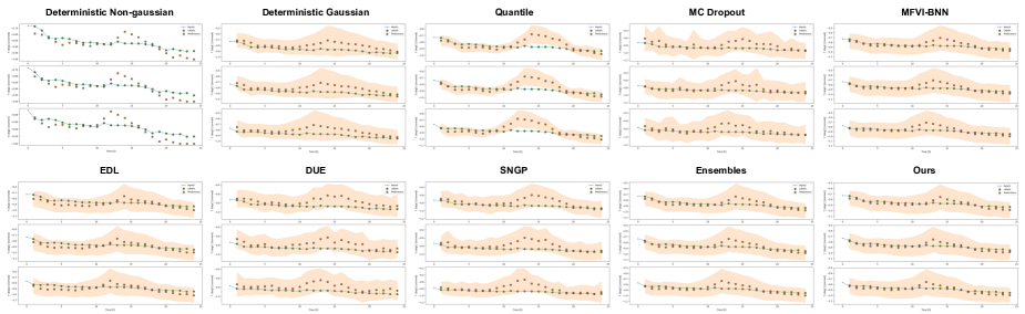
Figure 7: Comparison between methods in terms of temperature in Celsius (normalized) for every hour on three days on IID data. Our Density-Regression is still certain on IID.

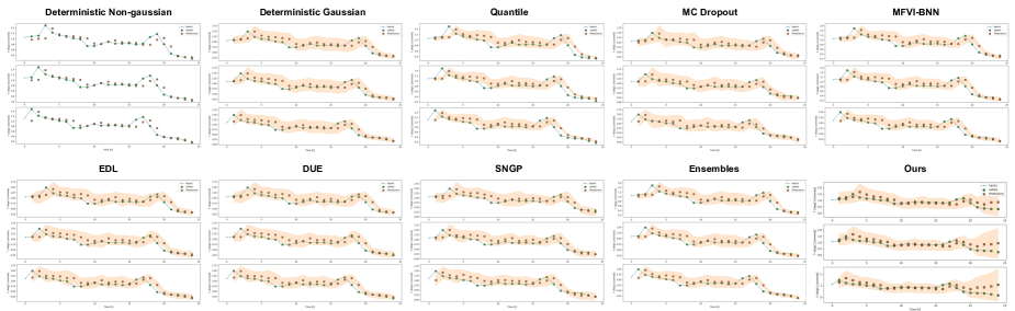
Figure 8: Comparison between methods in terms of temperature in Celsius (normalized) for every hour on three days on OOD data. Our Density-Regression is more uncertain on OOD.

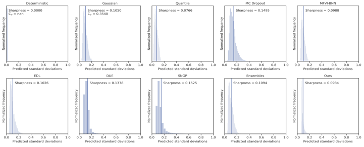
Figure 9: Detailed visualization of regression error, parity plot, calibration curve, and distribution plots with sharpness on the IID Time series weather forecasting.

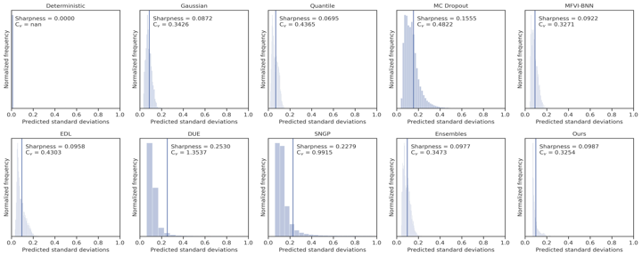
Figure 10: Detailed visualization of regression error, parity plot, calibration curve, and distribution plots with sharpness on the OOD Time series weather forecasting.

C.3 Benchmark UCI

Table 5: UCI: Boston housing

Method	NLL ($\downarrow$)	RMSE ($\downarrow$)	Cal ($\downarrow$)	Sharp ($\downarrow$)
Deterministic	2.64 $\pm$ 0.26	3.05 $\pm$ 0.21	0.39 $\pm$ 0.25	0.45 $\pm$ 0.08
Quantile	2.73 $\pm$ 0.75	3.03 $\pm$ 0.19	0.95 $\pm$ 0.49	0.30 $\pm$ 0.02
MC Dropout	2.42 $\pm$ 0.09	3.03 $\pm$ 0.26	0.54 $\pm$ 0.14	0.49 $\pm$ 0.06
MFVI-BNN	6.06 $\pm$ 0.51	10.9 $\pm$ 1.82	6.51 $\pm$ 0.71	17.2 $\pm$ 5.58
EDL	2.35 $\pm$ 0.06	3.02 $\pm$ 0.21	0.41 $\pm$ 0.19	0.76 $\pm$ 0.23
SNGP	2.37 $\pm$ 0.06	4.62 $\pm$ 0.33	0.42 $\pm$ 0.42	0.49 $\pm$ 0.03
DUE	2.35 $\pm$ 0.09	3.21 $\pm$ 0.28	0.41 $\pm$ 0.28	0.44 $\pm$ 0.05
Ensembles	2.30 $\pm$ 0.07	2.91 $\pm$ 0.11	0.25 $\pm$ 0.16	0.40 $\pm$ 0.03
Ours	2.46 $\pm$ 0.04	2.93 $\pm$ 0.11	0.22 $\pm$ 0.12	0.37 $\pm$ 0.01

Table 6: UCI: Concrete

Method	NLL ($\downarrow$)	RMSE ($\downarrow$)	Cal ($\downarrow$)	Sharp ($\downarrow$)
Deterministic	3.02 $\pm$ 0.09	5.58 $\pm$ 0.92	0.71 $\pm$ 0.78	0.39 $\pm$ 0.06
Quantile	3.24 $\pm$ 0.14	5.94 $\pm$ 0.54	1.04 $\pm$ 1.22	0.30 $\pm$ 0.03
MC Dropout	3.23 $\pm$ 0.05	6.33 $\pm$ 0.39	0.48 $\pm$ 0.38	0.50 $\pm$ 0.07
MFVI-BNN	6.93 $\pm$ 0.18	17.2 $\pm$ 4.51	8.64 $\pm$ 1.15	20.5 $\pm$ 6.13
EDL	3.03 $\pm$ 0.14	5.18 $\pm$ 0.5	2.24 $\pm$ 0.34	3.23 $\pm$ 2.26
SNGP	3.45 $\pm$ 0.07	7.59 $\pm$ 0.57	0.63 $\pm$ 0.61	0.56 $\pm$ 0.04
DUE	3.47 $\pm$ 0.07	7.82 $\pm$ 0.58	0.48 $\pm$ 0.45	0.56 $\pm$ 0.06
Ensembles	2.93 $\pm$ 0.04	4.82 $\pm$ 0.18	0.44 $\pm$ 0.24	0.37 $\pm$ 0.03
Ours	2.97 $\pm$ 0.08	4.94 $\pm$ 0.48	0.23 $\pm$ 0.33	0.30 $\pm$ 0.01

Table 7: UCI: Energy

Method	NLL ($\downarrow$)	RMSE ($\downarrow$)	Cal ($\downarrow$)	Sharp ($\downarrow$)
Deterministic	1.95 $\pm$ 0.27	2.18 $\pm$ 0.11	1.10 $\pm$ 1.40	0.21 $\pm$ 0.01
Quantile	1.91 $\pm$ 0.51	2.21 $\pm$ 0.16	1.15 $\pm$ 1.01	0.18 $\pm$ 0.02
MC Dropout	2.11 $\pm$ 0.08	2.94 $\pm$ 0.09	0.59 $\pm$ 0.64	0.36 $\pm$ 0.05
MFVI-BNN	3.14 $\pm$ 0.57	3.00 $\pm$ 0.15	1.77 $\pm$ 1.40	6.99 $\pm$ 2.31
EDL	1.64 $\pm$ 0.12	2.23 $\pm$ 0.13	3.05 $\pm$ 2.33	12.1 $\pm$ 4.12
SNGP	1.77 $\pm$ 0.11	2.18 $\pm$ 0.18	0.82 $\pm$ 0.82	0.27 $\pm$ 0.02
DUE	1.90 $\pm$ 0.09	2.61 $\pm$ 0.24	0.57 $\pm$ 0.64	0.29 $\pm$ 0.04
Ensembles	1.53 $\pm$ 0.07	2.14 $\pm$ 0.07	0.67 $\pm$ 0.54	0.24 $\pm$ 0.02
Ours	1.56 $\pm$ 0.13	2.15 $\pm$ 0.09	0.77 $\pm$ 0.84	0.22 $\pm$ 0.02

Table 8: UCI: Kin8nm

Method	NLL ($\downarrow$)	RMSE ($\downarrow$)	Cal ($\downarrow$)	Sharp ($\downarrow$)
Deterministic	-1.17 $\pm$ 0.03	0.08 $\pm$ 0.00	0.13 $\pm$ 0.15	0.30 $\pm$ 0.02
Quantile	-1.08 $\pm$ 0.05	0.08 $\pm$ 0.00	0.54 $\pm$ 0.42	0.26 $\pm$ 0.02
MC Dropout	-0.91 $\pm$ 0.02	0.11 $\pm$ 0.01	0.31 $\pm$ 0.17	0.53 $\pm$ 0.02
MFVI-BNN	-0.03 $\pm$ 0.11	0.18 $\pm$ 0.03	1.58 $\pm$ 1.57	5.12 $\pm$ 2.00
EDL	-1.07 $\pm$ 0.05	0.08 $\pm$ 0.00	0.83 $\pm$ 0.00	9.99 $\pm$ 0.30
SNGP	-1.05 $\pm$ 0.02	0.09 $\pm$ 0.00	0.18 $\pm$ 0.09	0.39 $\pm$ 0.01
DUE	-1.02 $\pm$ 0.02	0.09 $\pm$ 0.00	0.16 $\pm$ 0.08	0.40 $\pm$ 0.01
Ensembles	-1.25 $\pm$ 0.02	0.08 $\pm$ 0.00	0.40 $\pm$ 0.33	0.33 $\pm$ 0.02
Ours	-1.22 $\pm$ 0.02	0.08 $\pm$ 0.00	0.11 $\pm$ 0.19	0.30 $\pm$ 0.01

Table 9: UCI: Naval propulsion plant

Method	NLL ($\downarrow$)	RMSE ($\downarrow$)	Cal ($\downarrow$)	Sharp ($\downarrow$)
Deterministic	-4.93 $\pm$ 0.62	0.00 $\pm$ 0.00	2.58 $\pm$ 1.39	0.30 $\pm$ 0.05
Quantile	-4.79 $\pm$ 0.21	0.00 $\pm$ 0.00	3.04 $\pm$ 1.12	0.39 $\pm$ 0.02
MC Dropout	-4.69 $\pm$ 0.07	0.00 $\pm$ 0.00	0.66 $\pm$ 0.34	0.52 $\pm$ 0.05
MFVI-BNN	-4.07 $\pm$ 0.11	0.03 $\pm$ 0.01	4.10 $\pm$ 0.42	1.61 $\pm$ 0.11
EDL	-5.37 $\pm$ 0.27	0.00 $\pm$ 0.00	8.25 $\pm$ 0.00	100 $\pm$ 0.00
SNGP	-4.05 $\pm$ 0.08	0.00 $\pm$ 0.00	0.54 $\pm$ 0.49	0.74 $\pm$ 0.02
DUE	-3.89 $\pm$ 0.10	0.01 $\pm$ 0.00	0.71 $\pm$ 0.44	0.77 $\pm$ 0.03
Ensembles	-5.68 $\pm$ 0.17	0.00 $\pm$ 0.00	2.52 $\pm$ 1.04	0.30 $\pm$ 0.03
Ours	-5.42 $\pm$ 0.09	0.00 $\pm$ 0.00	2.29 $\pm$ 0.96	0.38 $\pm$ 0.01

Table 10: UCI: Power plant

Method	NLL ($\downarrow$)	RMSE ($\downarrow$)	Cal ($\downarrow$)	Sharp ($\downarrow$)
Deterministic	2.85 $\pm$ 0.03	4.03 $\pm$ 0.08	0.19 $\pm$ 0.18	0.24 $\pm$ 0.02
Quantile	3.03 $\pm$ 0.03	4.38 $\pm$ 0.05	0.34 $\pm$ 0.11	0.19 $\pm$ 0.01
MC Dropout	2.85 $\pm$ 0.02	4.22 $\pm$ 0.08	0.22 $\pm$ 0.24	0.27 $\pm$ 0.01
MFVI-BNN	4.02 $\pm$ 0.10	4.55 $\pm$ 0.31	10.7 $\pm$ 7.58	9.11 $\pm$ 3.04
EDL	2.82 $\pm$ 0.02	4.07 $\pm$ 0.08	8.21 $\pm$ 0.07	9.61 $\pm$ 6.72
SNGP	2.81 $\pm$ 0.01	4.10 $\pm$ 0.06	0.12 $\pm$ 0.09	0.25 $\pm$ 0.01
DUE	2.84 $\pm$ 0.02	4.19 $\pm$ 0.08	0.18 $\pm$ 0.26	0.26 $\pm$ 0.01
Ensembles	2.78 $\pm$ 0.01	3.99 $\pm$ 0.05	0.18 $\pm$ 0.18	0.23 $\pm$ 0.01
Ours	2.80 $\pm$ 0.02	4.02 $\pm$ 0.06	0.11 $\pm$ 0.12	0.22 $\pm$ 0.02

Table 11: UCI: Protein

Method	NLL ($\downarrow$)	RMSE ($\downarrow$)	Cal ($\downarrow$)	Sharp ($\downarrow$)
Deterministic	2.90 $\pm$ 0.02	4.63 $\pm$ 0.07	0.17 $\pm$ 0.09	0.76 $\pm$ 0.02
Quantile	3.19 $\pm$ 0.15	5.19 $\pm$ 0.04	3.26 $\pm$ 0.21	0.60 $\pm$ 0.01
MC Dropout	2.94 $\pm$ 0.07	4.85 $\pm$ 0.02	0.23 $\pm$ 0.08	3.76 $\pm$ 1.01
MFVI-BNN	3.68 $\pm$ 0.53	5.97 $\pm$ 0.55	3.54 $\pm$ 1.87	4.19 $\pm$ 1.44
EDL	3.20 $\pm$ 0.22	5.01 $\pm$ 0.45	3.50 $\pm$ 0.10	9.16 $\pm$ 3.22
SNGP	2.82 $\pm$ 0.01	4.57 $\pm$ 0.02	0.14 $\pm$ 0.04	0.78 $\pm$ 0.01
DUE	2.86 $\pm$ 0.02	4.69 $\pm$ 0.04	0.16 $\pm$ 0.07	0.79 $\pm$ 0.02
Ensembles	2.83 $\pm$ 0.01	4.58 $\pm$ 0.01	0.12 $\pm$ 0.04	0.79 $\pm$ 0.02
Ours	2.84 $\pm$ 0.01	4.61 $\pm$ 0.02	0.10 $\pm$ 0.04	0.73 $\pm$ 0.01

Table 12: UCI: Yacht

Method	NLL ($\downarrow$)	RMSE ($\downarrow$)	Cal ($\downarrow$)	Sharp ($\downarrow$)
Deterministic	1.29 $\pm$ 0.28	2.29 $\pm$ 0.56	0.93 $\pm$ 0.66	0.15 $\pm$ 0.03
Quantile	2.58 $\pm$ 0.93	3.90 $\pm$ 0.26	2.13 $\pm$ 1.72	0.17 $\pm$ 0.04
MC Dropout	1.82 $\pm$ 0.13	2.76 $\pm$ 0.38	2.19 $\pm$ 0.65	0.28 $\pm$ 0.03
MFVI-BNN	9.40 $\pm$ 1.14	22.6 $\pm$ 6.26	7.68 $\pm$ 0.39	28.9 $\pm$ 4.01
EDL	1.12 $\pm$ 0.16	2.48 $\pm$ 0.53	1.42 $\pm$ 1.25	0.30 $\pm$ 0.07
SNGP	1.16 $\pm$ 0.17	6.53 $\pm$ 0.49	1.29 $\pm$ 0.87	0.49 $\pm$ 0.05
DUE	1.22 $\pm$ 0.26	4.56 $\pm$ 1.23	1.38 $\pm$ 1.02	0.40 $\pm$ 0.08
Ensembles	1.18 $\pm$ 0.10	2.22 $\pm$ 0.21	2.02 $\pm$ 0.32	0.17 $\pm$ 0.02
Ours	1.24 $\pm$ 0.19	2.20 $\pm$ 0.42	0.87 $\pm$ 0.56	0.15 $\pm$ 0.03

Table 13: UCI: Year Prediction MSD

Method	NLL ($\downarrow$)	RMSE ($\downarrow$)	Cal ($\downarrow$)	Sharp ($\downarrow$)
Deterministic	3.49 $\pm$ 0.01	9.65 $\pm$ 0.07	0.06 $\pm$ 0.04	0.46 $\pm$ 0.02
Quantile	3.45 $\pm$ 0.01	9.46 $\pm$ 0.04	0.12 $\pm$ 0.02	0.37 $\pm$ 0.01
MC Dropout	3.50 $\pm$ 0.01	10.3 $\pm$ 0.08	0.07 $\pm$ 0.01	57.5 $\pm$ 4.49
MFVI-BNN	4.21 $\pm$ 0.10	11.5 $\pm$ 0.97	0.25 $\pm$ 0.04	26.1 $\pm$ 5.12
EDL	4.09 $\pm$ 0.22	11.2 $\pm$ 0.90	0.22 $\pm$ 0.08	21.1 $\pm$ 8.05
SNGP	3.52 $\pm$ 0.01	11.2 $\pm$ 0.17	0.12 $\pm$ 0.08	0.58 $\pm$ 0.01
DUE	3.53 $\pm$ 0.06	11.3 $\pm$ 0.81	0.10 $\pm$ 0.03	0.59 $\pm$ 0.04
Ensembles	3.35 $\pm$ 0.01	9.31 $\pm$ 0.03	0.06 $\pm$ 0.03	0.48 $\pm$ 0.02
Ours	3.39 $\pm$ 0.00	9.57 $\pm$ 0.02	0.04 $\pm$ 0.02	0.40 $\pm$ 0.01

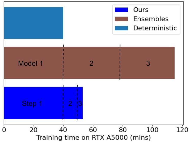
Table 14: Training time comparison between Deterministic, Ensembles, and Ours on the depth estimation setting.

References

- Tran et al. (2022) Dustin Tran, Jeremiah Liu, Michael W. Dusenberry, Du Phan, Mark Collier, Jie Ren, Kehang Han, Zi Wang, Zelda Mariet, Huiyi Hu, Neil Band, Tim G. J. Rudner, Karan Singhal, Zachary Nado, Joost van Amersfoort, Andreas Kirsch, Rodolphe Jenatton, Nithum Thain, Honglin Yuan, Kelly Buchanan, Kevin Murphy, D. Sculley, Yarin Gal, Zoubin Ghahramani, Jasper Snoek, and Balaji Lakshminarayanan. Plex: Towards reliability using pretrained large model extensions, 2022.
- Nado et al. (2021) Zachary Nado, Neil Band, Mark Collier, Josip Djolonga, Michael Dusenberry, Sebastian Farquhar, Angelos Filos, Marton Havasi, Rodolphe Jenatton, Ghassen Jerfel, Jeremiah Liu, Zelda Mariet, Jeremy Nixon, Shreyas Padhy, Jie Ren, Tim Rudner, Yeming Wen, Florian Wenzel, Kevin Murphy, D. Sculley, Balaji Lakshminarayanan, Jasper Snoek, Yarin Gal, and Dustin Tran. Uncertainty Baselines: Benchmarks for uncertainty & robustness in deep learning. arXiv preprint arXiv:2106.04015, 2021.
- Guo et al. (2017) Chuan Guo, Geoff Pleiss, Yu Sun, and Kilian Q. Weinberger. On calibration of modern neural networks. In Proceedings of the 34th International Conference on Machine Learning, 2017.
- Kuleshov et al. (2018) Volodymyr Kuleshov, Nathan Fenner, and Stefano Ermon. Accurate uncertainties for deep learning using calibrated regression. In Proceedings of the 35th International Conference on Machine Learning, 2018.
- Kuleshov and Deshpande (2022) Volodymyr Kuleshov and Shachi Deshpande. Calibrated and sharp uncertainties in deep learning via density estimation. In Proceedings of the 39th International Conference on Machine Learning, 2022.
- Minderer et al. (2021) Matthias Minderer, Josip Djolonga, Rob Romijnders, Frances Hubis, Xiaohua Zhai, Neil Houlsby, Dustin Tran, and Mario Lucic. Revisiting the calibration of modern neural networks. In Advances in Neural Information Processing Systems, 2021.
- Bui et al. (2021) Manh-Ha Bui, Toan Tran, Anh Tran, and Dinh Phung. Exploiting domain-specific features to enhance domain generalization. In Advances in Neural Information Processing Systems, 2021.
- Koh et al. (2021) Pang Wei Koh, Shiori Sagawa, Henrik Marklund, Sang Michael Xie, Marvin Zhang, Akshay Balsubramani, Weihua Hu, Michihiro Yasunaga, Richard Lanas Phillips, Irena Gao, Tony Lee, Etienne David, Ian Stavness, Wei Guo, Berton Earnshaw, Imran Haque, Sara M Beery, Jure Leskovec, Anshul Kundaje, Emma Pierson, Sergey Levine, Chelsea Finn, and Percy Liang. Wilds: A benchmark of in-the-wild distribution shifts. In Proceedings of the 38th International Conference on Machine Learning, 2021.
- Lakshminarayanan et al. (2017) Balaji Lakshminarayanan, Alexander Pritzel, and Charles Blundell. Simple and scalable predictive uncertainty estimation using deep ensembles. In Advances in Neural Information Processing Systems, 2017.
- Chen et al. (2016) Xiangli Chen, Mathew Monfort, Anqi Liu, and Brian D. Ziebart. Robust covariate shift regression. In Proceedings of the 19th International Conference on Artificial Intelligence and Statistics, 2016.
- Romano et al. (2019) Yaniv Romano, Evan Patterson, and Emmanuel Candes. Conformalized quantile regression. In Advances in Neural Information Processing Systems, 2019.
- Liu et al. (2020) Jeremiah Liu, Zi Lin, Shreyas Padhy, Dustin Tran, Tania Bedrax Weiss, and Balaji Lakshminarayanan. Simple and principled uncertainty estimation with deterministic deep learning via distance awareness. In Advances in Neural Information Processing Systems, 2020.
- van Amersfoort et al. (2022) Joost van Amersfoort, Lewis Smith, Andrew Jesson, Oscar Key, and Yarin Gal. On feature collapse and deep kernel learning for single forward pass uncertainty, 2022.
- Sensoy et al. (2018) Murat Sensoy, Lance Kaplan, and Melih Kandemir. Evidential deep learning to quantify classification uncertainty. In Advances in Neural Information Processing Systems, 2018.
- Charpentier et al. (2022) Bertrand Charpentier, Oliver Borchert, Daniel Zügner, Simon Geisler, and Stephan Günnemann. Natural posterior network: Deep bayesian predictive uncertainty for exponential family distributions. In International Conference on Learning Representations, 2022.
- Chua et al. (2018) Kurtland Chua, Roberto Calandra, Rowan McAllister, and Sergey Levine. Deep reinforcement learning in a handful of trials using probabilistic dynamics models. In Advances in Neural Information Processing Systems, 2018.
- Tran et al. (2020) Kevin Tran, Willie Neiswanger, Junwoong Yoon, Qingyang Zhang, Eric Xing, and Zachary W Ulissi. Methods for comparing uncertainty quantifications for material property predictions. Machine Learning: Science and Technology, 2020.
- Gneiting et al. (2007) Tilmann Gneiting, Fadoua Balabdaoui, and Adrian E. Raftery. Probabilistic Forecasts, Calibration and Sharpness. Journal of the Royal Statistical Society Series B: Statistical Methodology, 2007.
- Bui and Liu (2024) Ha Manh Bui and Anqi Liu. Density-softmax: Efficient test-time model for uncertainty estimation and robustness under distribution shifts, 2024.
- Charpentier et al. (2020) Bertrand Charpentier, Daniel Zügner, and Stephan Günnemann. Posterior network: Uncertainty estimation without ood samples via density-based pseudo-counts. In Advances in Neural Information Processing Systems, 2020.
- Vapnik (1998) Vladimir N. Vapnik. Statistical Learning Theory. Wiley-Interscience, 1998.
- Dinh et al. (2017) Laurent Dinh, Jascha Sohl-Dickstein, and Samy Bengio. Density estimation using real NVP. In International Conference on Learning Representations, 2017.
- Papamakarios et al. (2021) George Papamakarios, Eric Nalisnick, Danilo Jimenez Rezende, Shakir Mohamed, and Balaji Lakshminarayanan. Normalizing flows for probabilistic modeling and inference. Journal of Machine Learning Research, 2021.
- Hernandez-Lobato and Adams (2015) Jose Miguel Hernandez-Lobato and Ryan Adams. Probabilistic backpropagation for scalable learning of bayesian neural networks. In Proceedings of the 32nd International Conference on Machine Learning, 2015.
- Abadi et al. (2015) Martín Abadi, Ashish Agarwal, Paul Barham, Eugene Brevdo, Zhifeng Chen, Craig Citro, Greg S. Corrado, Andy Davis, Jeffrey Dean, Matthieu Devin, Sanjay Ghemawat, Ian Goodfellow, Andrew Harp, Geoffrey Irving, Michael Isard, Yangqing Jia, Rafal Jozefowicz, Lukasz Kaiser, Manjunath Kudlur, Josh Levenberg, Dandelion Mané, Rajat Monga, Sherry Moore, Derek Murray, Chris Olah, Mike Schuster, Jonathon Shlens, Benoit Steiner, Ilya Sutskever, Kunal Talwar, Paul Tucker, Vincent Vanhoucke, Vijay Vasudevan, Fernanda Viégas, Oriol Vinyals, Pete Warden, Martin Wattenberg, Martin Wicke, Yuan Yu, and Xiaoqiang Zheng. TensorFlow: Large-scale machine learning on heterogeneous systems, 2015. Software available from tensorflow.org.
- Amini et al. (2020) Alexander Amini, Wilko Schwarting, Ava Soleimany, and Daniela Rus. Deep evidential regression. In Advances in Neural Information Processing Systems, 2020.
- Cortez et al. (2009) P. Cortez, Antonio Luíz Cerdeira, Fernando Almeida, Telmo Matos, and José Reis. Modeling wine preferences by data mining from physicochemical properties. Decis. Support Syst., 2009.
- Ronneberger et al. (2015) Olaf Ronneberger, Philipp Fischer, and Thomas Brox. U-net: Convolutional networks for biomedical image segmentation. In Medical Image Computing and Computer-Assisted Intervention – MICCAI 2015. Springer International Publishing, 2015.
- Silberman et al. (2012) Nathan Silberman, Derek Hoiem, Pushmeet Kohli, and Rob Fergus. Indoor segmentation and support inference from rgbd images. In Computer Vision – ECCV 2012. Springer Berlin Heidelberg, 2012.
- Goodfellow et al. (2015) Ian Goodfellow, Jonathon Shlens, and Christian Szegedy. Explaining and harnessing adversarial examples. In International Conference on Learning Representations, 2015.
- Huang et al. (2018) Xinyu Huang, Xinjing Cheng, Qichuan Geng, Binbin Cao, Dingfu Zhou, Peng Wang, Yuanqing Lin, and Ruigang Yang. The apolloscape dataset for autonomous driving. In 2018 IEEE/CVF Conference on Computer Vision and Pattern Recognition Workshops (CVPRW), 2018.
- Bui and Maifeld-Carucci (2022) Ha Manh Bui and Iliana Maifeld-Carucci. Benchmark for uncertainty & robustness in self-supervised learning, 2022.
- Ovadia et al. (2019) Yaniv Ovadia, Emily Fertig, Jie Ren, Zachary Nado, D. Sculley, Sebastian Nowozin, Joshua Dillon, Balaji Lakshminarayanan, and Jasper Snoek. Can you trust your model's uncertainty? evaluating predictive uncertainty under dataset shift. In Advances in Neural Information Processing Systems, 2019.
- Hendrycks and Dietterich (2019) Dan Hendrycks and Thomas Dietterich. Benchmarking neural network robustness to common corruptions and perturbations. In International Conference on Learning Representations, 2019.
- Gustafsson et al. (2023) Fredrik K. Gustafsson, Martin Danelljan, and Thomas B. Schön. How reliable is your regression model’s uncertainty under real-world distribution shifts? Transactions on Machine Learning Research, 2023.
- Dheur and Ben Taieb (2023) Victor Dheur and Souhaib Ben Taieb. A large-scale study of probabilistic calibration in neural network regression. In Proceedings of the 40th International Conference on Machine Learning, 2023.
- Gardner et al. (2018) Jacob Gardner, Geoff Pleiss, Kilian Q Weinberger, David Bindel, and Andrew G Wilson. Gpytorch: Blackbox matrix-matrix gaussian process inference with gpu acceleration. In Advances in Neural Information Processing Systems, 2018.
- Lee et al. (2018) Jaehoon Lee, Jascha Sohl-dickstein, Jeffrey Pennington, Roman Novak, Sam Schoenholz, and Yasaman Bahri. Deep neural networks as gaussian processes. In International Conference on Learning Representations, 2018.
- Blundell et al. (2015) Charles Blundell, Julien Cornebise, Koray Kavukcuoglu, and Daan Wierstra. Weight uncertainty in neural networks. In Proceedings of the 32nd International Conference on Machine Learning, 2015.
- Wen et al. (2018) Yeming Wen, Paul Vicol, Jimmy Ba, Dustin Tran, and Roger Grosse. Flipout: Efficient pseudo-independent weight perturbations on mini-batches. In International Conference on Learning Representations, 2018.
- Gal and Ghahramani (2016a) Yarin Gal and Zoubin Ghahramani. Dropout as a bayesian approximation: Representing model uncertainty in deep learning. In Proceedings of The 33rd International Conference on Machine Learning, 2016a.
- Gal and Ghahramani (2016b) Yarin Gal and Zoubin Ghahramani. A theoretically grounded application of dropout in recurrent neural networks. In Advances in Neural Information Processing Systems, 2016b.
- Gal et al. (2017) Yarin Gal, Jiri Hron, and Alex Kendall. Concrete dropout. In Advances in Neural Information Processing Systems, 2017.
- Hansen and Salamon (1990) L.K. Hansen and P. Salamon. Neural network ensembles. IEEE Transactions on Pattern Analysis and Machine Intelligence, 1990.
- Wen et al. (2020) Yeming Wen, Dustin Tran, and Jimmy Ba. Batchensemble: an alternative approach to efficient ensemble and lifelong learning. In International Conference on Learning Representations, 2020.
- Dusenberry et al. (2020) Michael Dusenberry, Ghassen Jerfel, Yeming Wen, Yian Ma, Jasper Snoek, Katherine Heller, Balaji Lakshminarayanan, and Dustin Tran. Efficient and scalable Bayesian neural nets with rank-1 factors. In Proceedings of the 37th International Conference on Machine Learning, 2020.
- Collier et al. (2021) Mark Collier, Basil Mustafa, Efi Kokiopoulou, Rodolphe Jenatton, and Jesse Berent. Correlated input-dependent label noise in large-scale image classification. In Proceedings of the IEEE/CVF Conference on Computer Vision and Pattern Recognition (CVPR), 2021.
- Koenker and Bassett (1978) Roger W Koenker and Jr Bassett, Gilbert. Regression Quantiles. Econometrica, 1978.
- Song et al. (2019) Hao Song, Tom Diethe, Meelis Kull, and Peter Flach. Distribution calibration for regression. In Proceedings of the 36th International Conference on Machine Learning, 2019.
- Vovk et al. (2005) Vladimir Vovk, Alex Gammerman, and Glenn Shafer. Algorithmic Learning in a Random World. Springer-Verlag, Berlin, Heidelberg, 2005. ISBN 0387001522.
- Tibshirani et al. (2019) Ryan J Tibshirani, Rina Foygel Barber, Emmanuel Candes, and Aaditya Ramdas. Conformal prediction under covariate shift. In Advances in Neural Information Processing Systems, 2019.
- Prinster et al. (2022) Drew Prinster, Anqi Liu, and Suchi Saria. Jaws: Auditing predictive uncertainty under covariate shift. In Advances in Neural Information Processing Systems, 2022.
- Prinster et al. (2023) Drew Prinster, Suchi Saria, and Anqi Liu. JAWS-x: Addressing efficiency bottlenecks of conformal prediction under standard and feedback covariate shift. In Proceedings of the 40th International Conference on Machine Learning, 2023.
- Chung et al. (2021) Youngseog Chung, Willie Neiswanger, Ian Char, and Jeff Schneider. Beyond pinball loss: Quantile methods for calibrated uncertainty quantification. In Advances in Neural Information Processing Systems, 2021.
- Mukhoti et al. (2020) Jishnu Mukhoti, Viveka Kulharia, Amartya Sanyal, Stuart Golodetz, Philip Torr, and Puneet Dokania. Calibrating deep neural networks using focal loss. In Advances in Neural Information Processing Systems, 2020.
- Mukhoti et al. (2023) Jishnu Mukhoti, Andreas Kirsch, Joost van Amersfoort, Philip HS Torr, and Yarin Gal. Deep deterministic uncertainty: A new simple baseline. In Proceedings of the IEEE/CVF Conference on Computer Vision and Pattern Recognition, 2023.
- Kotelevskii et al. (2022) Nikita Kotelevskii, Aleksandr Artemenkov, Kirill Fedyanin, Fedor Noskov, Alexander Fishkov, Artem Shelmanov, Artem Vazhentsev, Aleksandr Petiushko, and Maxim Panov. Nonparametric uncertainty quantification for single deterministic neural network. In Advances in Neural Information Processing Systems, 2022.
- Nalisnick et al. (2019) Eric Nalisnick, Akihiro Matsukawa, Yee Whye Teh, Dilan Gorur, and Balaji Lakshminarayanan. Do deep generative models know what they don’t know? In International Conference on Learning Representations, 2019.
- Steinwart and Christmann (2011) Ingo Steinwart and Andreas Christmann. Estimating conditional quantiles with the help of the pinball loss. Bernoulli, 2011.
Acronyms
- AI
- Artificial Intelligence
- BNN
- Bayesian Neural Network
- DNN
- Deep Neural Network
- DUE
- Deterministic Uncertainty Estimation
- EDL
- Evidential Deep Learning
- ERM
- Empirical Risk Minimization
- GP
- Gaussian Process
- IID
- Independent-identically-distributed
- MC
- Monte-Carlo
- MFVI
- Mean-Field Variational Inference
- MLE
- Maximum Likelihood Estimation
- NatPN
- Natural Posterior Network
- NLL
- Negative log-likelihood
- OOD
- Out-of-Distribution
- RMSE
- Root Mean Square Error
- SNGP
- Spectral-normalized Neural Gaussian Process
- SOTA
- State-of-the-art
Glossary