Unitary quantum gravitational physics and the CMB parity asymmetry
Abstract
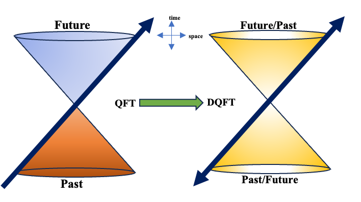
The proposal of Direct-Sum Quantum Field Theory (DQFT) offers a new perspective for quantum fields by combining parity and time reversal operations, blurring the distinction between quantum past and future while preserving causality. This approach provides a unitary QFT in curved spacetime, resolving the information-loss paradox. When applied to inflationary quantum fluctuations, DQFT predicts variations in CMB measurements, explaining longstanding anomalies as a result of parity asymmetry. The data strongly supports the unitary treatment of quantum fluctuations, with a probability over 650 times greater than the standard prediction. This significant discrepancy underscores the validity and importance of the DQFT approach in understanding the intricate relationship between gravity and quantum mechanics.
Introduction - Understanding and testing the interplay between gravity and quantum mechanics (QM) is the most important key to unraveling the new physics beyond the standard model of particle physics and Einstein’s general relativity (GR). The merge of GR and QM is an essential physics to be unlocked at the length scales of gravitational horizons. For this, we perhaps need an in-depth understanding of how one can resolve an age-old conundrum in the concept of time between the GR and QM. The success of Quantum field theory (QFT) in Minkowski spacetime Coleman (2018) already teaches us several lessons in this regard. Indeed QFT is the culmination of special relativity (SR) and QM where the concept of time already enters into the conflict. In SR, the space and time are on equal footing but in QM spatial coordinates are elevated to operators while time is just a parameter due to its anti-unitary nature under discrete transformation (). The SR and QM are merged by imposing the commutativity of operators corresponding to space-like distances. The underlying reason is that SR forbids any sort of communication happening in space-like distances and we respect it and achieve it in formulating the rules of second quantization. This is exactly the lesson one must keep in mind for understanding quantum fields in curved spacetime. That is we take lessons from classical physics and apply them according to the rules of quantum physics. The quantum field theory in curved spacetime (QFTCS) is the first step in seeing GR and QM together besides the renormalizable ultra-violet complete quantum gravity that may be required at the Planck scales. Furthermore, QFTCS is a necessity in the context of understanding inflationary quantum fluctuations Mukhanov and Chibisov (1981); Sasaki (1986).
In this letter, we address crucial questions related to the meaning of time reversal and parity inversions in the context of inflationary background spacetime to place quantum fields on it and uncover their true nature in the cosmic microwave background (CMB). We explain how the direct-sum quantum field theory (DQFT) is a necessity to resolve the unitarity and information-loss problem of QFTCS. The question of unitarity in QFTCS precedes the question of a completely renormalizable quantum gravity theory of Planck scales. In contrast to the widespread schools of thought that argue unitarity in QFTCS needs to be given up within GR and QM, we came up with a fundamental understanding of it and an observational test of it by the remarkable revelation of parity asymmetry in the CMB. We find that the theory of inflationary quantum fluctuations with DQFT (which we call shortly DSI which stands for ”Direct-Sum inflation”) fits up to 650 times better than the Standard Inflation (SI). This letter ultimately presents the picture of how a new theory of QFTCS emerged from fundamental questions of quantum gravitational physics that can potentially explain the observed CMB large-scale anomalies. The new results in this letter are further complemented with our companion paper Gaztañaga and Sravan Kumar (2024).
DQFT, in a nutshell, ()- DQFT formulation emerges from a simple demand that a quantum state or a quantum field operator respects the discrete symmetries (Parity and time reversal ) of the background spacetime. Here we summarize the conceptual understanding of DQFT and direct the reader to Gaztañaga and Sravan Kumar (2024); Sravan Kumar and Marto (2023a, b) for more details. We start with the direct-sum Schrödinger equation
| (1) |
where is the time-independent Hamiltonian (which is Hermitian) that is symmetric. The quantum state is the direct-sum of two components
| (2) | ||||
where are the two components of the same state at parity conjugate points. The component is a positive energy state that evolves forward in time as where the parametric time arrow while the can also be seen as positive energy state that evolves back in time as with the parametric time convention . One can notice here the purely anti-unitary character of time associated with the replacement Donoghue and Menezes (2019). The direct-sum Schrödinger equation does not have any arrow of time associated with it in comparison to the conventional Schrödinger equation. The direct-sum splitting of the quantum state (2) implies the Hilbert space splitting into a direct-sum of the two corresponding to parity conjugate points in position space: . The position and momentum commutation relations now become double associated with parity conjugate position and momentum space operators denoted by subscripts and their relations are
| (3) | ||||
This framework only makes the wavefunction of the quantum system explicitly symmetric that resonates with the assumed symmetry of the physical system i.e., and the results of standard quantum mechanics remains the same as shown with the example of harmonic oscillator worked out in Gaztañaga and Sravan Kumar (2024). The DQFT in Minkowski spacetime ( which is symmetric) is just built on the direct-sum Schrödinger equation, following how standard QFT is built. See Appendix A for more details and Fig.1 for an illustration.
DQFT in curved spacetime, gravitational horizons unitarity and information-loss paradox ()- The de Sitter (dS) spacetime is a perfect testing ground for exploring the theory of QFTCS because of its maximally symmetric aspect and it is also relevant for unlocking the nature of inflationary quantum fluctuations. Furthermore, dS spacetime has the closest resemblance with black holes where the most important conundrums in quantum physics emerge such as the loss of unitarity and information-loss paradox.
We start with the dS metric in the flat Friedman-Lemaître-Robertson-Walker (FLRW) coordinates
| (4) |
where the scale factor is the clock that determines the expansion of the Universe, is the Hubble parameter and is the conformal time. If one has to place quantum theory in dS spacetime (4) the first and foremost things to be understood are the parity and time reversal operations. The usual conception of understanding the expansion of the Universe is to restrict to . But the metric carries a symmetry
| (5) |
and restricting to before quantization of a classical field (as it is usually followed in standard QFTCS) means throwing away the symmetry by hand (5). The expanding Universe can be realized in two ways:
| (6) |
This would explain why in the Wheeler-de Witt equation the cosmic time does not explicitly appear, rather the scale factor is the clock that runs with expanding Universe Kiefer (2007). Note that does not change at all any properties of dS space. For example, curvature invariants such as Ricci scalar remain the same under discrete sign flip of H. The equation (6) illustrates two possible time realizations for an expanding universe. By convention, choosing or results in information loss beyond the horizon. Schrödinger in his famous monograph of 1956 Erwin Schrodinger (1956) rejected the idea of two Universes because it would lead to a conundrum of ignorance of information beyond the horizon which in modern language pure states evolving into mixed states which leads the violation of unitarity and information-loss Gibbons and Hawking (1977); Parikh et al. (2003).
Similar to the Minkowski space (see Appendix A), the quantum fields in the dS space are created in a direct-sum vacuum corresponding to the direct-sum Fock space . This implies, that everywhere in dS space a quantum field is tied by time forward and backward evolutions at the parity conjugate points, see Appendix B. At any moment of dS expansion, the parity-conjugate points on the comoving horizon are space-like separated for an imaginary classical observer as shown in Fig. 2.
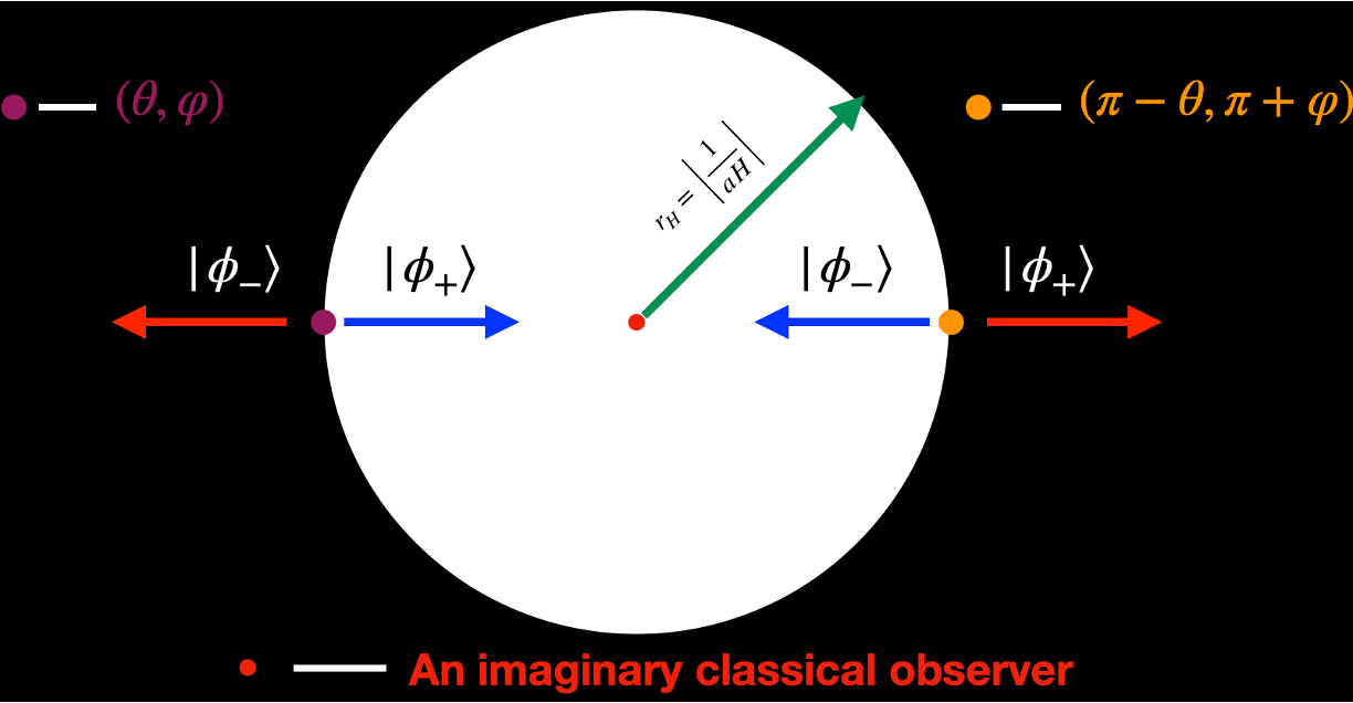
Note that by DQFT construction, the direct-sum quantum states that follow from (20) are the opposite time evolving positive energy states at the parity conjugate points and this holds for any imaginary classical observer. Furthermore, DQFT preserves the causality and locality too. A consequence of this is that any state that disappears beyond the horizon happens to be a direct-sum state that reappears at the antipodal point. This is because all the imaginary classical observers including those on the horizons of each other should observe the same direct-sum quantum states .
This means the horizon acts as a mirror which maps every information outside the horizon to the states inside the horizon. Fig. 2 gives the pictorial representation of this. This feature of DQFT implies any maximally entangled state (a pure state)
| (7) |
remains within the horizon because no information is lost beyond the horizon. Every information of each of the entanglement pairs is mapped to within the horizon, thus the pure state will remain a pure state. In other words, DQFT forbids any entanglement beyond the gravitational horizons. DQFT constructs a direct-sum Hilbert space with the interior and exterior being separated by a superselection rule Wick et al. (1952); nLab authors (2023). Thus, there would be an observer complementarity. We can also understand the same from the point of view of dS space in static coordinates which reads as
| (8) | ||||
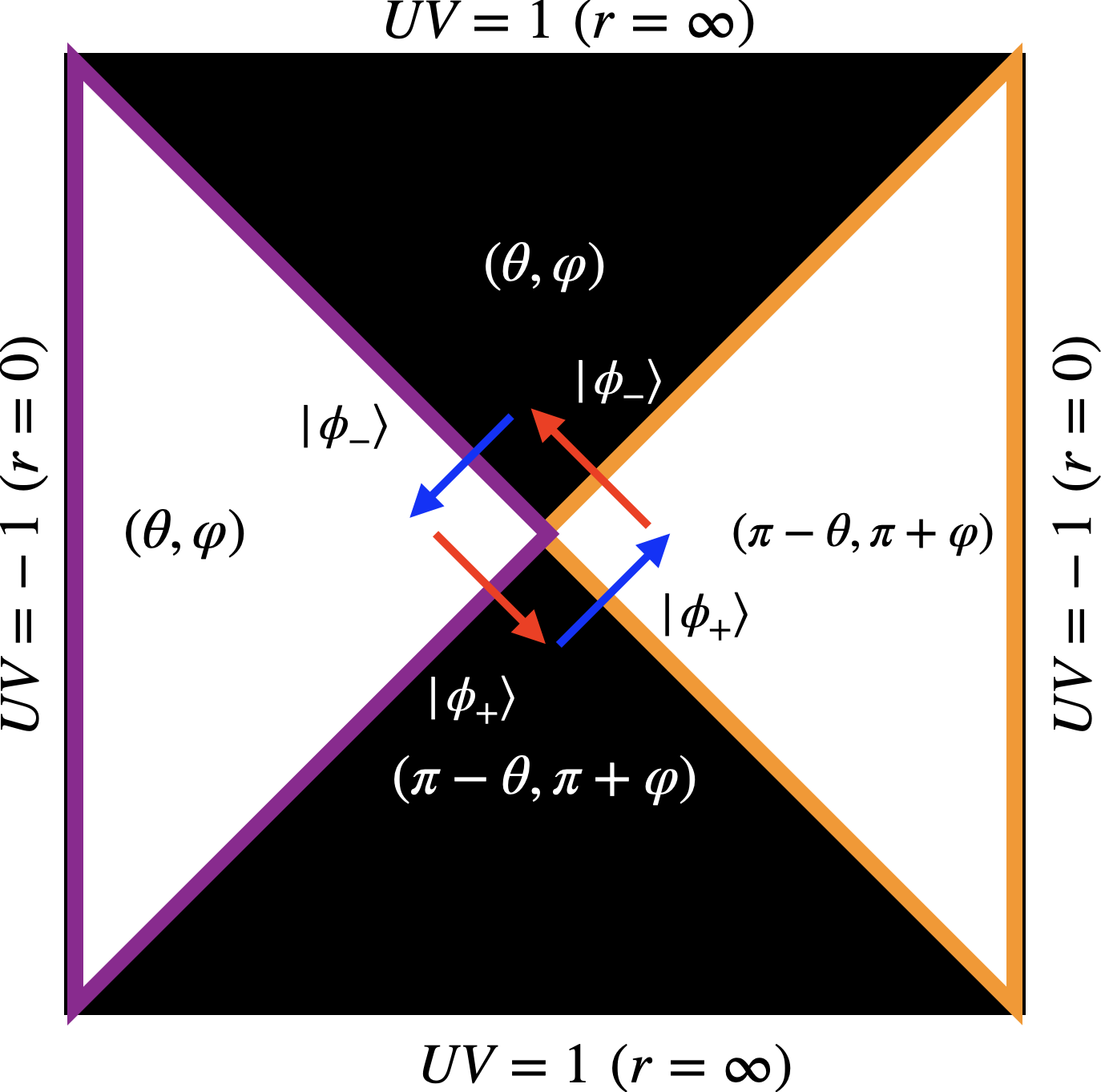
where and . The relation between the flat FLRW (4) and (8) is just a simple coordinate change Lanczos and Hoenselaers (1997); Hartman (2017). A very practiced view of flat dS spacetime (4) is that it covers only half of the dS space. But we must keep in mind the symmetry (6) which implies that (4) can cover the entire dS space. Thus the maximally symmetric nature of dS spacetime sets no difference whether it is expressed in flat, closed, open FLRW coordinates or the static coordinates Mukhanov and Winitzki (2007). The use of mapping flat coordinates to static coordinates here is that we can realize how unitarity can be achieved with DQFT whereas it is lost in the standard QFT as it was shown by Gibbons and Hawking in 1977 Gibbons and Hawking (1977). In Fig. 3, we show the unitary quantum physics in the static dS space through the conformal (not) Penrose diagram, where we see the three-dimensional space split by parity for the interior (the white region) and exterior (the dark region) of the cosmological event horizon. We can picture here how none of the observers lose any information beyond the horizon. If any state leaves the horizon it is only the direct-sum component of what is inside the horizon. This means any observer can perfectly reconstruct information about what is beyond the horizon. Any state beyond the horizon is not entangled with what is inside. This means the Hilbert spaces of the interior and exterior states cannot be connected by direct-product () but rather should be related by direct-sum (). This has to be like this because beyond-the-horizon time is not the same, so one cannot do the same quantum mechanics everywhere. In other words, the gravitational horizons are special, they separate different spacetimes by a boundary. Thus, they cannot be treated as a standard null surface where quantum states can be entangled across. Furthermore, we stress that no entanglement across the horizon does not lead to firewalls which happens in standard QFTCS but not in direct-sum QFTCS. We suggest Ref. Sravan Kumar and Marto (2023b) to the reader for further analogous discussion on unitarity and no information loss in the context of the Schwarzschild black hole. In a nutshell, DQFT offers a new understanding of dS space where any observer’s physics of the universe is complete, and no information is lost outside any observer’s Universe. This is exactly what Schrödinger envisioned a quantum theory to achieve in 1956 Erwin Schrodinger (1956). Furthermore, our achievement of DQFT echoes well with the recent classical understanding of dS through the Black Hole Universe (BHU) proposal Gaztanaga (2022); Gaztañaga (2023).
Direct-sum Inflation (DSI) and CMB parity asymmetry - Inflationary quantum fluctuations are the initial seeds for large-scale structure formation. It is important to understand their quantum nature to derive consistent CMB predictions. Inflation is by definition a quasi-dS expansion Starobinsky (1980) and this means that (6) is spontaneously broken by the presence of a non-perturbative scalar field in addition to the GR’s tensor degree of freedom. Our focus here is on single-field inflation. The metric and scalar field matter quantum fluctuations are generated during inflation. The quantity which is a gauge invariant combination of them is called the curvature perturbation (), and it is an effective (scalar) degree of freedom. It connects the quantum physics of inflation to CMB observations. The action for curvature perturbation at the linear order is
| (9) |
where which is nearly constant during inflation characterized by the smallness of slow-roll parameters for number of e-foldings. The canonical variable which is a redefinition of curvature perturbation that we eventually quantize is
| (10) |
In the framework of DSI, the canonical variable is promoted to field operator that is split into direct-sum of two components
| (11) |
which generate quantum fields in a direct-sum vacuum
| (12) |
in which they evolve forward and backward in time at the parity conjugate points in physical space. In analogy with (6), the time reversal operation (quantum mechanically) in an expanding quasi-dS Universe is
| (13) |
The CMB provides temperature fluctuations all over the sky :
| (14) |
the Fourier coefficients are characterized by the angular power spectrum . Because (and is broken by the slow-roll parameters (13), we expect the quantum field during inflation to evolve time asymmetrically at parity conjugate points in physical space. This leads to an angular power spectrum of the CMB exhibiting an excess of power in the odd multipoles compared to the even ones, as described by (21) in Appendix C.
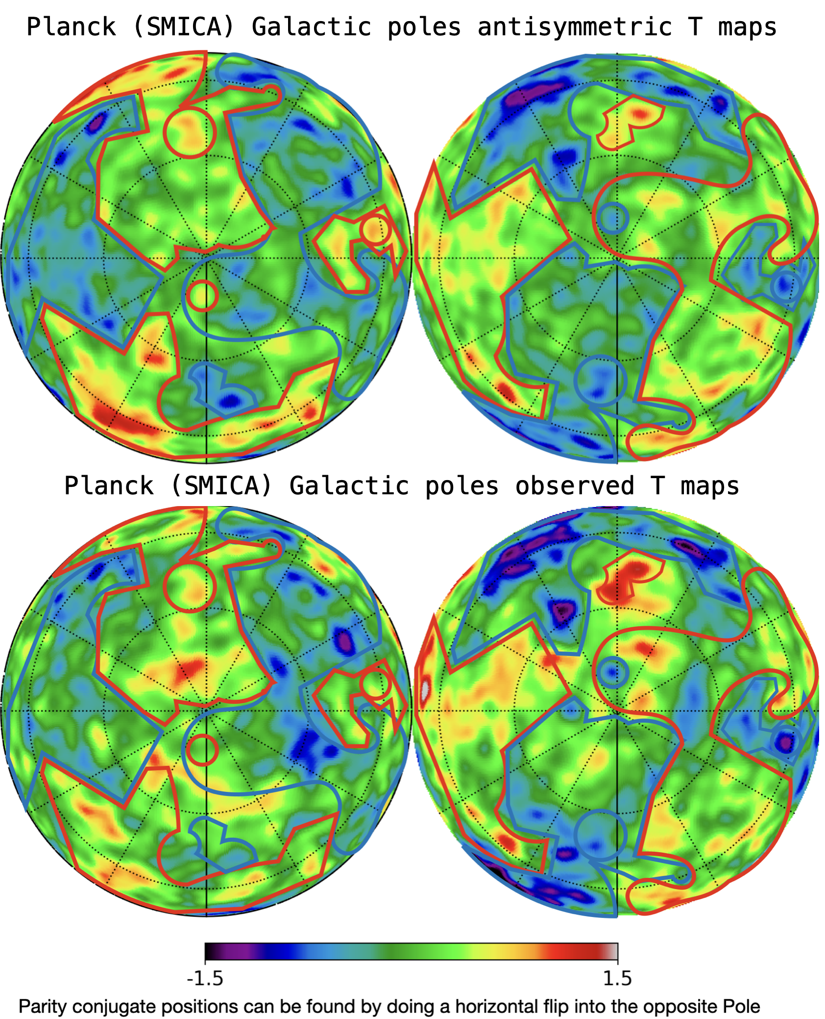
In Fig. 4 we can see visually the parity asymmetry by the close resemblance between odd parity temperature maps and the original CMB maps from Planck data Akrami et al. (2020a). This reflects that the Planck temperature maps contain an additional pure odd parity component. The DSI framework exactly generates this additional odd symmetry as we can see in (21). It is worth noticing here that if we take the average of even and odd power spectra we recover the well-known near-scale invariant power spectrum of Standard Inflation (SI). The benefit of DSI is that there are no additional free parameters. The parity asymmetry just depends on the spectral index at the scale ( or ) as measured by the Planck data Akrami et al. (2020b).
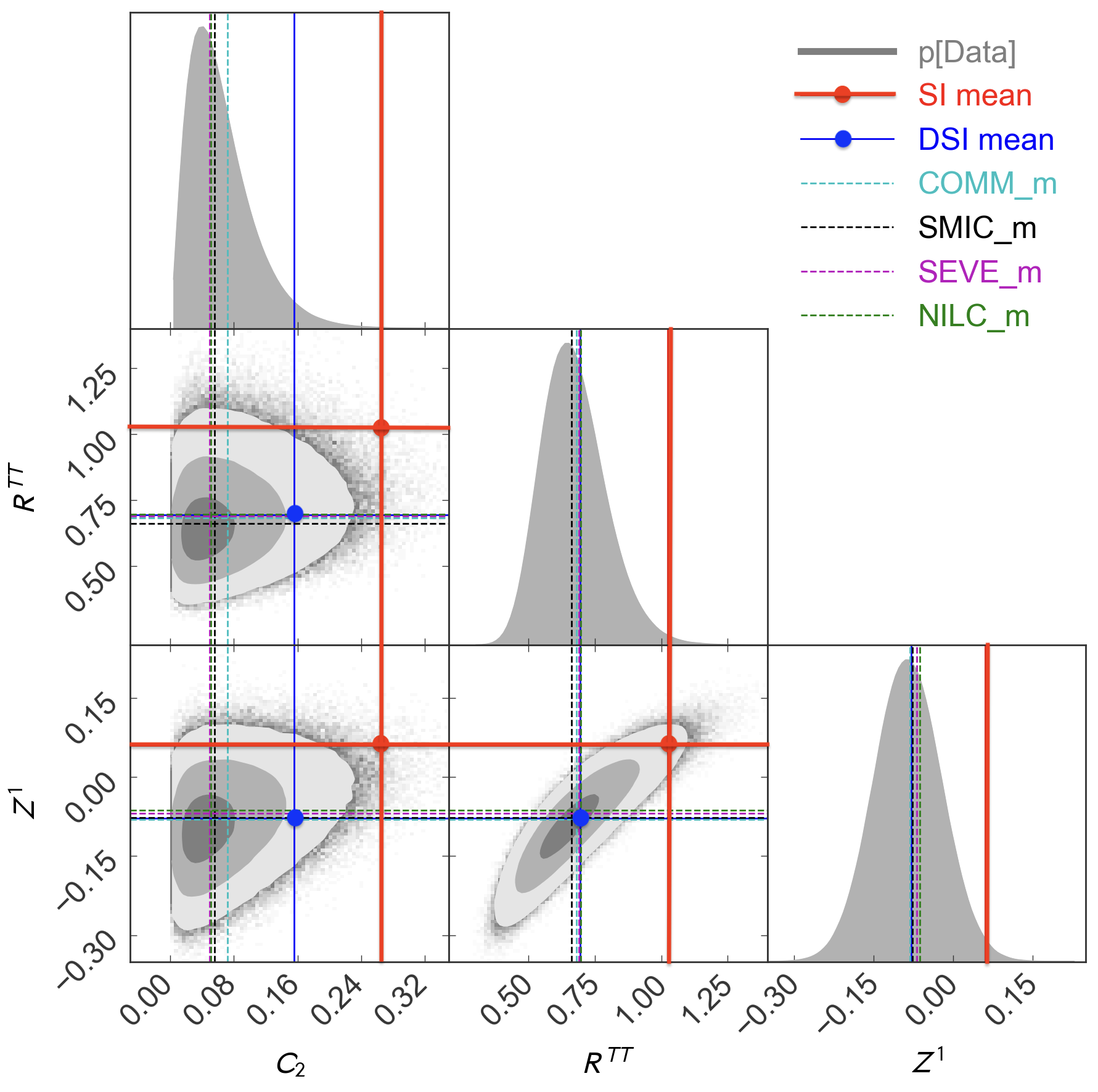
In Fig. 6 we present how the observational data prefers significantly DSI over SI. Observed quantities include the observed low quadrupolar amplitude , the even-to-odd multipole ratio of angular power spectra:
| (15) |
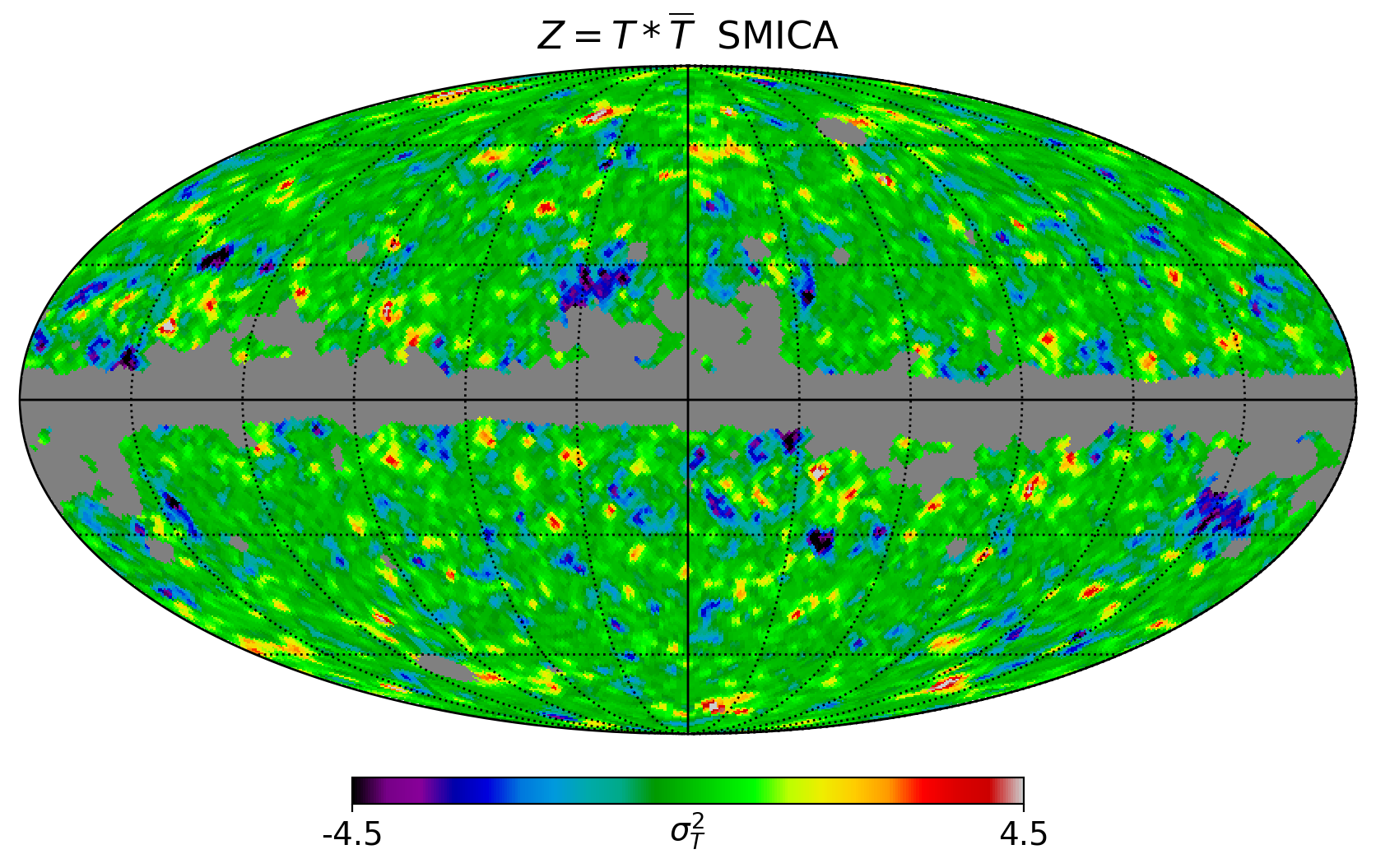
and the mean of the parity map displayed in Fig.5, where represents the parity conjugate or antipode of the sky position . The likelihood probability associated with DSI in these plots is up to 650 times larger than that of SI. DSI favors odd parity, leading to a lower . This, in turn, diminishes the significance of other CMB anomalies Schwarz et al. (2016), such as the Hemispherical Power Asymmetry, the axis of Evil, and the anomalous 2-point correlation function (See Gaztañaga and Sravan Kumar (2024) for further details).
Conclusions- In this letter, we underscore the pivotal role of unitary Quantum Field Theory in Curved Spacetime (QFTCS) in elucidating the intricacies of early Universe physics. Contrary to prevailing notions, we contend that the issue of unitarity in QFTCS is not inherently tied to quantum gravity at Planck scales, but rather stems from our incomplete comprehension of quantum fields in curved spacetime.
With the -symmetric formulation of Schrödinger equation (1), the DQFT framework reinstates unitarity, which was previously thought to be lost in curved spacetime. Fig. 2-3 visually represent this concept, illustrating how a hypothetical classical observer consistently experiences pure states without encountering information loss beyond the horizon.
Furthermore, the striking correlation illustrated in Fig. 4-6 between the observed hot and cold mirrored structures of the CMB map at antipodal points strongly supports the unitary treatment of inflationary quantum fluctuations within the framework of DQFT. Our findings indicate that superhorizon fluctuations at antipodes manifest as conjugates, a prediction derived from direct-sum QFTCS. This prediction is substantially favored with a probability over 650 times greater than that of the standard QTFCS.
Acknowledgements.
EG acknowledges grants from Spain Plan Nacional (PGC2018-102021-B-100) and Maria de Maeztu (CEX2020-001058-M). KSK acknowledges the Royal Society for the Newton International Fellowship.References
- Coleman (2018) S. Coleman, Lectures of Sidney Coleman on Quantum Field Theory, edited by B. G.-g. Chen, D. Derbes, D. Griffiths, B. Hill, R. Sohn, and Y.-S. Ting (WSP, Hackensack, 2018).
- Mukhanov and Chibisov (1981) V. F. Mukhanov and G. V. Chibisov, JETP Lett. 33, 532 (1981), [Pisma Zh. Eksp. Teor. Fiz.33,549(1981)].
- Sasaki (1986) M. Sasaki, Prog. Theor. Phys. 76, 1036 (1986).
- Gaztañaga and Sravan Kumar (2024) E. Gaztañaga and K. Sravan Kumar, arXiv e-prints 10.48550/arXiv.2401.08288 (2024).
- Sravan Kumar and Marto (2023a) K. Sravan Kumar and J. Marto, arXiv e-prints , arXiv:2305.06046 (2023a).
- Sravan Kumar and Marto (2023b) K. Sravan Kumar and J. Marto, arXiv e-prints 10.48550/arXiv.2307.10345 (2023b).
- Donoghue and Menezes (2019) J. F. Donoghue and G. Menezes, Phys. Rev. Lett. 123, 171601 (2019), arXiv:1908.04170 [hep-th] .
- Kiefer (2007) C. Kiefer, Quantum Gravity, 2nd ed. (Oxford University Press, New York, 2007).
- Erwin Schrodinger (1956) Erwin Schrodinger, Expanding universes, Cambridge University Press (1956).
- Gibbons and Hawking (1977) G. W. Gibbons and S. W. Hawking, Phys. Rev. D 15, 2738 (1977).
- Parikh et al. (2003) M. K. Parikh, I. Savonije, and E. P. Verlinde, Phys. Rev. D 67, 064005 (2003), arXiv:hep-th/0209120 .
- Wick et al. (1952) G. C. Wick, A. S. Wightman, and E. P. Wigner, Phys. Rev. 88, 101 (1952).
- nLab authors (2023) nLab authors, superselection theory, https://ncatlab.org/nlab/show/superselection+theory (2023), .
- Lanczos and Hoenselaers (1997) K. Lanczos and C. Hoenselaers, GR and Gravitation 29, 361 (1997).
- Hartman (2017) T. Hartman, Lecture Notes on Classical de Sitter Space (2017).
- Mukhanov and Winitzki (2007) V. Mukhanov and S. Winitzki, Introduction to quantum effects in gravity (Cambridge University Press, 2007).
- Gaztanaga (2022) E. Gaztanaga, Universe 8, 257 (2022).
- Gaztañaga (2023) E. Gaztañaga, MNRAS 521, L59 (2023).
- Starobinsky (1980) A. A. Starobinsky, Phys. Lett. B91, 99 (1980).
- Akrami et al. (2020a) Y. Akrami et al. (Planck), Astron. Astrophys. 641, A7 (2020a).
- Akrami et al. (2020b) Y. Akrami et al. (Planck), Astron. Astrophys. 641, A10 (2020b), arXiv:1807.06211 [astro-ph.CO] .
- Schwarz et al. (2016) D. J. Schwarz, C. J. Copi, D. Huterer, and G. D. Starkman, Class. Quant. Grav. 33, 184001 (2016).
Appendix A Appendix A: Klein-Gordon field operator in DQFT
The Klein-Gordon field operator for DQFT in Minkowski spacetime split into direct-sum
| (16) |
where
| (17) |
where . The creation and annihilation operators satisfy the canonical relations
| (18) |
which defines the positive norm states in the direct-sum vacuums . The DQFT splits the Fock space as the direct-sum of two Fock spaces corresponding to the field’s components where states of forward in time and backward in time at parity conjugate regions of position space can be created and annihilated by the pair of operators (18). Since the Minkowski spacetime is symmetric the scalar field operator in DQFT respects the same symmetry. For further details on DQFT and invariance see Sravan Kumar and Marto (2023a).
Appendix B Appendix B: DQFT in dS
Applying DQFT in dS Gaztañaga and Sravan Kumar (2024); Sravan Kumar and Marto (2023a), by construction the scalar field operator is the direct-sum of two components
| (19) |
where
| (20) |
Here the operators satisfy the similar relations like in (18). The dS mode functions corresponding to the standard Bunch-Davies vacuum of the DQFT.
Appendix C Appendix C: DSI angular power spectrum
Following Gaztañaga and Sravan Kumar (2024), the CMB power spectrum in DSI is:
| (21) | ||||
where , and
| (22) |
Here, are the Hankel and Bessel functions of the first kind, and is the cut-scale we impose as (22) is accurate enough for low- or large angular scales. This cut-off scale is also related to the coarse gaining scale of stochastic inflation Gaztañaga and Sravan Kumar (2024) which determines the large wavelength modes that have already become classical on the onset of inflation while the mode exiting the horizon. In DSI, these large wavelength modes create parity asymmetric inhomogeneities that correct the FLRW spacetime on large scales. The parity asymmetry ceases to exist towards the small scales because the symmetry recovered towards the short distance scales. This can be seen in Fig. 11 of Gaztañaga and Sravan Kumar (2024). An intuitive explanation for this is that large wavelength modes experience quantum gravitational effects more than those of short wavelength modes.