Abstract

Spatially resolved relative phase measurement of two adjacent 1D Bose gases is enabled by matter-wave interference upon free expansion. However, longitudinal dynamics is typically ignored in the analysis of experimental data. We provide an analytical formula showing a correction to the readout of the relative phase due to longitudinal expansion and mixing with the common phase. We numerically assess the error propagation to the estimation of the gases’ physical quantities such as correlation functions and temperature. Our work characterizes the reliability and robustness of interferometric measurements, directing us to the improvement of existing phase extraction methods necessary to observe new physical phenomena in cold-atomic quantum simulators.

Contents

1. 1 Introduction
2. 2 Free expansion dynamics of parallel 1D Bose gases
3. 3 Readout phase error due to longitudinal expansion
4. 4 Reconstruction of physical quantities
   1. 4.1 Correlation functions
   2. 4.2 Full Distribution Functions
   3. 4.3 Velocity-velocity correlation
   4. 4.4 Mean occupation number & temperature
5. 5 Summary & Discussion
6. 6 Acknowledgments
7. A Free expansion dynamics
8. B Derivation of the transverse fit formula
9. C Corrections due to longitudinal dynamics
10. D Relative phase fitting initialization
11. E Additional plots

1 Introduction

Matter-wave interference [1] not only highlights the quantum nature of matter but also provides ultra precise sensors for metrology and serves as a sensitive probe for the intricate many body physics of ultracold quantum gases and quantum simulators [2]. A key technique thereby is time-of-flight (TOF) measurements, where the quantum gas expands upon being released from the trap. If two such expanded clouds overlap, they form a matter-wave interference pattern from which the relative phase between the trapped clouds can be extracted. If the expansion preserves local information, properties connected to the relative local phase in the original samples can be extracted.

This rational was extensively used in particular for 1D cold-atomic quantum field simulators to study non-equilibrium dynamics [3], prethermalization [4, 5], area law scaling of the mutual information[6], and quantum thermodynamics [7, 8]. This is because the statistical properties of relative phases [9] can be used to infer physical quantities of the gas such as temperature [10], relaxation time scales [11, 12]; the nature of excitations through full distribution functions [13, 14] and quantum tomography [15]; the quantum field theory description through correlation functions [16, 17]; and the propagation of information [18, 19].

In this work, we perform a focused study on the TOF measurement of two parallel 1D Bose gases, going beyond the initial idealized reasoning in [20, 21]. We systematically address a variety of different physical phenomena that can modify the interference patterns and thereby the extraction of the local relative phase. We assess the accuracy of the decoding, i.e. the inference of the relative phase in the trapped clouds from the observed interference. Such a detailed and systematic analysis of the various effects that can influence TOF measurement becomes indispensable when pushing further the detailed analysis of low dimensional many body quantum systems and the quantum field simulators they enable.

To reliably extract the relative phase, we need an accurate understanding of the measurement dynamics. If the trap is switched off rapidly, the dynamics are well approximated by a quench into free evolution [20, 21], which leads to the gas expanding ballistically while free falling. For 1D systems, such free expansion can be divided into expansion in the transversal directions (perpendicular to the length of the gas) and longitudinal direction (along the length of the gas). Although previous studies [22, 23] often neglect longitudinal expansion, recent theoretical works have started to address its significance [21, 24, 25]. In particular, they unveil new phenomena affecting the formation of interference patterns such as density ripples [20], and mixing with common (symmetric) phases [21, 24]. A natural question then arises: How do these factors influence the relative phase extraction fidelity and the determination of gases’ physical properties? To the best of our knowledge, no systematic answer has been offered in the literature. This paper therefore aims to comprehensively address this question.

The paper is structured as follows: after a brief introduction in Sec. 1, we summarize the developments in modelling TOF measurement dynamics for parallel 1D systems in Sec. 2. In Sec. 3 we develop a perturbative theory for incorporating longitudinal dynamics, and derive analytical expressions for the systematic readout errors in the extracted phase. Sec. 4 provide numerical analyses to assess the influence of errors on the estimation of the various physical quantities of the gases, accounting for modelling errors (Sec. 4). We conclude with a brief discussion and outloook in Sec. 5.

2 Free expansion dynamics of parallel 1D Bose gases

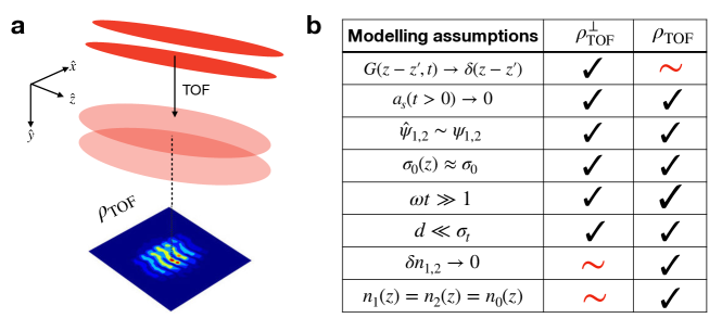
Figure 1: (a) The setup schematics for relative phase measurement of parallel (quasi-)one dimensional Bose gases (red) after time of flight (TOF) adapted from Ref. [26] (b) Comparison table for the assumptions used to derive different models for TOF density [Eqs. (4)-(5)]. The $\sim$ symbol means that the assumption can be relaxed in general.

We consider a pair of parallel one-dimensional bosonic gases of length $L$ extending along the $z$-axis (longitudinal axis) and separated by a distance $d$ along one of the transversal axes, e.g. the $x$-axis [Fig. 1a]. Let $\hat{\psi}_{j}(z)$ be the bosonic annihilation operator with subscripts $j=1,2$ indexing the left and right well respectively. This operator can be decomposed as $\hat{\psi}_{j}(z)=e^{i\hat{\phi}_{j}}\sqrt{\hat{n}_{j}}$ with $\hat{n}_{j}$ and $\hat{\phi}_{j}$ being the density and phase operators. In this paper, we will use the semi-classical approximation by replacing $\hat{\psi}_{j}(z)$ with a scalar field $\psi_{j}(z)=e^{i\phi_{j}(z)}\sqrt{n_{j}(z)+\delta n_{j}(z)}$ where $n_{j}(z)$ is the mean density, and $\delta n_{j}(z),\phi_{j}(z)$ are density and phase fluctuations respectively. The objective of 1D Bose gases interferometry is to measure the relative phase fluctuation $\phi_{-}(z)=\phi_{2}(z)-\phi_{1}(z)$. This can be achieved through TOF scheme, whereby the atomic cloud is imaged after being released and expanded for some time $t$. The image encodes information about the in-situ phase fluctuations in the resulting interference pattern of the expanded density measured in experiments.

In the following, we assume the system to be initially in the quasi-1D regime, i.e. only occupying the Gaussian transverse ground state wavefunction [27, 28, 22]

$$\Psi_{j}(x,y,z,0)=\frac{1}{\sqrt{\pi\sigma_{0}^{2}(z)}}\exp\left(-\frac{(x\pm d/2)^{2}+y^{2}}{2\sigma_{0}(z)^{2}}\right)\psi_{j}(z),$$ (1)

where the right and left wells are assumed to be symmetric with respect to the origin. The Gaussian width $\sigma_{0}^{2}(z)=\sigma_{0}^{2}\sqrt{1+2a_{s}n_{j}(z)}$ depends on the scattering length $a_{s}$, the mean density $n_{j}(z)$, and the single-particle ground state width $\sigma_{0}=\sqrt{\hbar/(m\omega)}$ given by the atomic mass $m$ and the transverse trapping frequency $\omega$. For the moment, we will ignore the radial broadening due to atomic repulsion such that the width $\sigma_{0}(z)\equiv\sigma_{0}$ is uniform along the condensate. We discuss the effect of scattering in Sec. 5 and Appendix E.

We model TOF expansion as a ballistic expansion, without any external potential nor any interaction (i.e. $a_{s}(t>0)=0$). The latter is justified due to the fast decrease of interaction energy as a result of the rapid expansion of the gas in the tightly confined transverse directions. Thus, for $t>0$ the system is effectively governed by free particle dynamics [20, 25, 21]

$$\Psi_{j}(\vec{r},z,t)=\int d^{2}\vec{r}^{\prime}\;dz^{\prime}\;G(\vec{r}-\vec{r}^{\prime},t)G(z-z^{\prime},t)\;\Psi_{j}(\vec{r}^{\prime},z^{\prime},0),$$ (2)

where $\vec{r}$ is a short-hand notation for the position vector in the transverse plane and $G(\xi,t)=\sqrt{\frac{m}{2\pi i\hbar t}}e^{-m\xi^{2}/2i\hbar t}$ is the free, single-particle Green’s function. We also note that a recent work [25] has developed a fast and efficient method to numerically evaluate Eq. (2). In our analytical contributions, we make use of additional approximations to obtain a simplified analytical form of the time evolution. Thus, our results are complementary to that of Ref. [25], while paving the way for a further systematic understanding of the TOF scheme.

As the gases expand, they start to overlap and coherently interfere. We are interested in the density image of the atomic cloud after interference as seen from the vertical direction ($y$-axis), i.e.

$$\rho_{\rm TOF}(x,z,t)=\int dy\;|\Psi_{1}(\vec{r},z,t)+\Psi_{2}(\vec{r},z,t)|^{2}.$$ (3)

After substituting the time-evolved fields from Eq. (2) and applying the assumptions listed in Fig. 1b, one arrives at a simplified formula for the expanded density [22, 23]

$$\rho_{\text{TOF}}^{\perp}(x,z,t)=A(z,t)e^{-x^{2}/\sigma_{t}^{2}}\Big{[}1+C(z)\cos\big{(}kx+\phi_{-}(z)\big{)}\Big{]},$$ (4)

where $\sigma_{t}=\sigma_{0}\sqrt{1+\omega^{2}t^{2}}$ is the expanded Gaussian width, $k(t)=d/(\sigma_{0}^{2}\omega t)=md/(\hbar t)$ is inverse fringe spacing, and $A(z,t)$ and $C(z)$ are interference peaks and contrasts respectively. In experiments, the relative phase $\phi_{-}(z)$ is obtained by fitting the interference image to Eq. (4), and so we refer to it as ‘transversal fit formula’. The superscript $\perp$ means we have ignored longitudinal dynamics by substituting $G(z-z^{\prime},t)\approx\delta(z-z^{\prime})$ in Eq. (2). In addition, the formula also assumes $\omega t\gg 1$ and $d\ll\sigma_{t}$ such that the overlapping transverse Gaussian can be approximated as a single Gaussian centred at the origin. Furthermore, although they can be relaxed, we consider identical mean density $n_{1}(z)=n_{2}(z)=n_{0}(z)$ and ignore density fluctuation $\delta n_{1,2}\ll n_{0}$.

This work explores the impact of longitudinal expansion on the accuracy of relative phase extraction. In other words, we go beyond Eq. (4) by including longitudinal dynamics in our analysis, where the final density after expansion and interference is written as [21]

$$\rho_{\text{TOF}}(x,z,t)=Ae^{-x^{2}/\sigma_{t}^{2}}\left|\int_{-L/2}^{L/2}dz^{\prime}\;G(z-z^{\prime},t)\sqrt{n_{0}(z^{\prime})}e^{i\phi_{+}(z^{\prime})/2}\cos\left(\frac{kx+\phi_{-}(z^{\prime})}{2}\right)\right|^{2},$$ (5)

where $\phi_{+}(z):=\phi_{1}(z)+\phi_{2}(z)$ is the common (symmetric) phase [24, 29], typically unmeasured in experiments. We provide a detailed derivation of Eq. (5) in Appendix A and we show how to recover Eq. (4) from Eq. (5) in Appendix B. The mixing with common degrees of freedom in Eq. (5) is a new phenomenon neglected in Eq. (4). Meanwhile, longitudinal expansion manifests itself through the Green’s function kernel which allows local correlation between density at $z$ and $z^{\prime}\neq z$. We refer to Eq. (5) as the ‘full expansion formula’. Unlike the transversal fit formula, the integral form and the dependence on the common phase make it difficult to use the full expansion formula as a fit function.

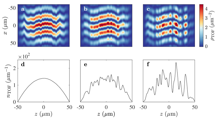
Figure 2: Comparison between three different TOF expansion models: (a) $\rho_{\rm TOF}^{\perp}$ , (b) $\rho_{\rm TOF}$ with $\phi_{+}(z)=0$, and (c) $\rho_{\rm TOF}$ with $\phi_{+}(z)\neq 0$. Panels d - f show the respective TOF longitudinal density $n_{\rm TOF}=\int\rho_{\rm TOF}\;dx$. The mean insitu density $n_{0}(z)$ is set to follow the Thomas-Fermi approximation in harmonic potential (inverse parabola) with peak density $75\;\rm{\mu m}^{-1}$. The other parameter values are $t=15\;\rm ms$, $\omega=2\pi\times 2\;\rm{kHz}$, $L=100\;\rm\mu m$, $d=3\;\mu m$, and $m$ is the mass of ${}^{87}\rm{Rb}$. These parameters are fixed throughout the paper unless stated otherwise.

We conclude our description of these models by illustrating their differences in Fig. 2a-c, showing a comparison between interference patterns of identical phase profiles computed with different expansion models. Their differences are visible through the longitudinal variation of the central peaks. They can also be seen more clearly by numerically evaluating longitudinal density $n_{\rm TOF}(z,t)=\int dx\;\rho_{\rm TOF}(x,z,t)$, which is directly measurable in experiments by imaging the atoms along the $x$-axis[22, 20, 10]. The result is shown in Figs. 2d-e with the transverse fit formula showing no density ripples [Fig. 2d], i.e. $n_{\rm TOF}(z)=n_{0}(z)$, in contrast with the full formula [Figs. 2e-f].

The density ripples imply the presence of systematic longitudinal correlations in the interference pattern induced by free expansion, which is neglected in the transversal expansion model. Since we read out the relative phase from the interference pattern, it is natural to ask whether this density correlation will cause a systematic correlation in the readout phase as well, leading to a systematic error between true insitu phase and the readout phase. This error is indeed numerically reported in Ref. [21] but with no systematic characterization of their behaviour. We will discuss this in the next section.

3 Readout phase error due to longitudinal expansion

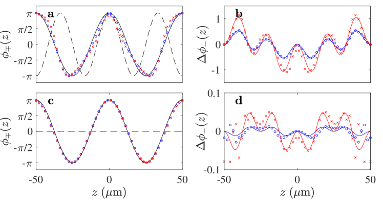
Figure 3: (a) Input relative (solid black line) and common (dashed black line) phase profiles $\phi_{-}(z)=\pi\cos(4\pi z/L)$ and $\phi_{+}(z)=\pi\cos(6\pi z/L)$ together with the extracted phase profiles $\phi_{-}^{\text{(out)}}(z)$ with $t=7\;\rm ms$ (blue circles) and $t=15\;\rm ms$ (red crosses). (b) Phase shift induced by longitudinal expansion $\Delta\phi_{-}(z,t)=\phi_{-}(z)-\phi_{-}^{\text{(out)}}(z)$. The solid lines are fitting curves based on Eq. (9). Panels c-d are repetition of a-b with $\phi_{+}(z)=0$. Numerical errors have been accounted for by subtracting the phase error using the transversal model in both encoding and decoding. The initial mean density profile is the same as in Fig. 2 (inverse parabola).

In experimental analysis, longitudinal dynamics are often ignored, and Eq. (4) is used to read out the relative phase from the density interference pattern. If we relax this assumption, the expression for the final density is given by Eq. (5), which is considerably more complicated and no longer useful as a fitting function. Our aim in this section is to assess the modelling error that may arise from ignoring longitudinal expansion. We do this by treating the integral in Eq. (5) perturbatively.

We start by defining an integrand function,

$$I(x,z^{\prime},t)\equiv\sqrt{n_{0}(z^{\prime})}e^{i\phi_{+}(z^{\prime})/2}\cos\left(\frac{kx+\phi_{-}(z^{\prime})}{2}\right),$$ (6)

so that the integral in Eq. (5) can be written as $\int_{-L/2}^{L/2}dz^{\prime}\;G(z-z^{\prime},t)I(x,z^{\prime},t)$. Similar the stationary phase approximation, the integrand’s dominant contribution will come from $z^{\prime}\approx z$. We may then perform asymptotic expansion of the integral around that point in analogy to Laplace’s method [30], i.e. we perform Taylor expansion of $I(x,z^{\prime},t)$ centred around $z$.

We show in Appendix C that up to second-order approximation, Eq. (5) can always be expressed in the following form

$$\rho_{\rm TOF}(x,z,t)\approx A^{\prime}(z,t)e^{-x^{2}/\sigma^{2}(t)}\left[1+C^{\prime}(z,t)\cos\left(kx+\phi_{-}(z)-\Delta\phi_{-}(z,t)\right)\right],$$ (7)

where $A^{\prime}(z,t),\;C^{\prime}(z,t)$ now include corrections from longitudinal expansion. The above implies that, at least up to the second order, longitudinal expansion does not change the functional relationship between $\rho_{\rm TOF}(x,z,t)$ and $\phi_{-}(z)$. This demonstrates the robustness of the transversal fit formula; nevertheless, longitudinal expansion still influences the extracted fit parameters. In particular, it introduces a systematic phase shift $\Delta\phi_{-}(z,t)$ into the readout phase, so that

$$\phi_{-}^{\rm(out)}(z,t)=\phi_{-}(z)-\Delta\phi_{-}(z,t).$$ (8)

For a uniform gas, the dominant corrections for the phase $\Delta\phi_{-}(z,t)$ are expressed in terms of scaled derivatives of the phases

$$\Delta\phi_{-}(z,t)=\frac{1}{2}(\partial_{\eta}\phi_{-})(\partial_{\eta}\phi_{+})+\frac{1}{8}(\partial_{\eta}^{2}\phi_{-})(\partial_{\eta}\phi_{-})^{2}+O(\partial_{\eta}^{4}),$$ (9)

where derivatives are taken with respect to a scaled coordinate $\eta=z/\ell_{t}$ with $\ell_{t}=\sqrt{\hbar t/m}$ being the length scale of longitudinal expansion. In the standard Bogoliubov theory for 1D gas [31], the scaled derivative of the phase with respect to a finite lattice length is considered a small parameter. Similarly, our formula is expanded with respect to small parameters $\partial_{\eta}\phi_{\pm}$ with $\ell_{t}$ being analogous to lattice length. The corrections to Eq. (9) are of order four or higher in scaled phase derivatives [see Appendix C].

Equations (7)-(9) are the main analytical results of this paper. In particular, Eq. (9) is useful to assess the reliability of the existing phase readout protocol. For example, it shows that the readout error grows with a longer expansion time. This is intuitive since a longer longitudinal expansion time would lead to a more systematic longitudinal correlation spread along the gas. Moreover, Eq. (9) also clearly shows a dominant phase shift correction due to mixing with the common phase, which was previously unnoticed. We also find a higher-order correction that depends only on the derivatives of the relative phase, signifying a systematic error purely due to the presence of longitudinal Green’s function.

We compare our analytical prediction with numerical data by encoding smooth phase profiles, e.g. $\phi_{-}(z)=\pi\cos(4\pi z/L)$ and $\phi_{+}(z)=\pi\cos(6\pi z/L)$, into density interference pattern computed with the full expansion formula and then decode the relative phase with the transverse fit formula. We find agreement between numerical data and our analytical prediction up to finite size effects near the boundary [Fig. 3]. We also examined the fit for various other smooth profiles and obtained similar results. Note that the numerical data does not assume uniform density and yet Eq. (9) fits the data quite well, demonstrating the usefulness of our formula in realistic scenarios where density varies sufficiently slowly.

4 Reconstruction of physical quantities

Ultimately, we are interested in reconstructing physical quantities associated with the gas’ initial state, which we assume to be given by a Hamiltonian of the form [20, 32]

$$H=H_{LL}(\delta\rho_{+},\phi_{+})+H_{LL}(\delta\rho_{-},\phi_{-})-2\hbar Jn_{0}\int dz\;\cos\phi_{-}(z)~{},$$ (10)

where $H_{LL}$ is the Luttinger-Liquid Hamiltonian. While the common mode is determined by this Gaussian theory, the non-Gaussianity of the relative degrees of freedom can be experimentally tuned via the single particle tunnelling strength $J$, giving rise to the sine-Gordon model. The relevance of the cosine potential can be characterized by $q=\lambda_{T}/l_{J}$ which is directly related to the experimentally accessible coherence factor $\langle\cos(\phi_{-})\rangle$. The thermal coherence length $\lambda_{T}=\hbar^{2}n_{\rm 1D}/(mk_{B}T)$ for uniform gas $n_{0}=n_{\rm 1D}$ and phase locking length $l_{J}=\frac{1}{2}\sqrt{\hbar/mJ}$ determine the randomization and restoration of the phase due to temperature and tunnel coupling respectively. In thermal equilibrium phase correlation functions for varying $q$, i.e. strength of the tunnel coupling $J$, have been experimentally computed up to the 10-th order [32] and found in agreement with predictions of the sine-Gordon model.

In this section, we assess the reliability of TOF measurement for such a task, especially in the light of possible error propagation from $\Delta\phi_{-}(z,t)$. To this aim, we will mainly resort to numerical simulation, where our workflow is summarized in Fig. 4.

• Independent sampling of relative and common phase profiles. We sample many instances of $\{\phi_{\mp}^{\rm(in)}(z)\}$ from a many body state. In our case, the many body state would either be a thermal Gaussian state or a non-Gaussian sine-Gordon state. The phase profiles corresponding to thermal Gaussian state are sampled from a multivariate normal distribution following a thermal covariance matrix [15], with small tunnelling $J=0.1\;Hz$ to renormalize the zero modes. Meanwhile, the non-Gaussian phase profiles are sampled by a stochastic process described by an Itô equation [33, 34].

  The sampled phase profiles are the input to our simulation. Using these inputs, the ground-truth physical quantities $\mathcal{O}\left(\left\{\phi_{-}^{\rm(in)}(z)\right\}\right)$ can be computed. Although it may contain statistical fluctuations, given sufficiently many samples of the phase profiles, the computed quantities $\mathcal{O}$ should closely match their theoretical values.

• Simulation of the TOF encoding of phases into density interference patterns. Given the phase profiles, we simulate TOF by computing density after TOF ($\rho_{\rm TOF}$) using Eq. (5) with varying expansion time $t$. To control for the influence of common phases, we perform the simulation twice for every $t$, once with zero common phase ($\phi_{+}(z)=0$) and the second time with the sampled common phase ($\phi_{+}(z)=\phi_{+}^{\rm(in)}(z)$). In addition, we simulate the transverse expansion model to control for numerical error in the relative phase decoding process (explained below).

• Decoding of interference patterns to extract relative phase. With the obtained $\rho_{\rm TOF}$, we use Eq. (4) as a fitting function to extract $\phi_{-}(z)$. To do so, we solve a constrained optimization $\phi_{-}^{\text{(out)}}(z)\in[-2\pi,2\pi]$ problem using the interior-point algorithm. We initialize the optimizer by feeding a linear function $\phi_{-}^{\text{(0)}}(z)=-kx_{\text{max}}$ where $x_{\text{max}}$ is the transversal peak position at fixed $z$ [Appendix D]. Due to phase multiplicity over a $2\pi$ period, we sometimes observe phase jumps (discontinuity) in the optimization output. We eliminate the discontinuity by applying a phase unwrapping protocol where we add a multiple of $2\pi$ to the phase whenever we detect a jump larger than $\pi$ until the discontinuity is eliminated. However, this protocol is inaccurate for highly fluctuating profiles in finite resolution, which puts a limit on the temperatures for which our method performs reliably.

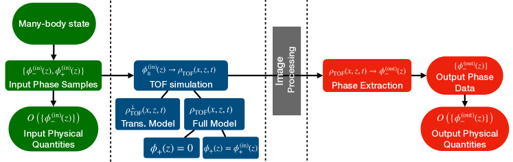
Figure 4: The simulation workflow is divided into four stages, separated by the dotted lines. The first stage (green boxes) represents the input to the simulation, obtained by sampling relative and common phase profiles from an input state. The next stage (blue boxes) represents TOF encoding implemented with three different models. The last stage (red boxes) represents decoding where relative phases and physical quantities are inferred by fitting with the transverse fit formula (4). The goal of the simulation is to compare the input and output physical quantities. Current progress is underway to further investigate the effects of image processing in the experimental setup, which will allow us to observe the interplay between modelling and experimental errors.

After obtaining all the decoded phases data $\{\phi_{-}^{\rm(out)}(z)\}$, we compute the inferred physical quantities $\mathcal{O}(\{\phi_{-}^{\rm(out)}(z)\})$ and compare them to the input $\mathcal{O}(\{\phi_{-}^{\rm(in)}(z)\})$ in different scenarios. Note that in Fig. 4, there is an additional image processing stage between the encoding and decoding process. This is the stage where the initial interference pattern gets modified due to the experimental setup and limitations of the imaging devices.

4.1 Correlation functions

Equal-time higher-order correlations contain detailed information about the many body state, and can be directly calculated from the extracted phase profiles after time of flight. Computing all correlation functions is tantamount to solving a many body problem  [32, 17, 22]. The $N$-th order relative phase correlation function referenced at $z=0$ is defined by

$$G^{(N)}(\mathbf{z})=\left\langle\prod_{i=1}^{N}\left(\phi_{-}(z_{i})-\phi_{-}(0)\right)\right\rangle\ ,$$ (11)

where $\mathbf{z}=(z_{1},z_{2},...,z_{N})$. In general, the correlation function can be decomposed into the connected and disconnected part

$$G^{(N)}(\mathbf{z})=G^{(N)}_{\rm con}(\mathbf{z})+G^{(N)}_{\rm dis}(\mathbf{z}).$$ (12)

The disconnected part can be expressed in terms of lower-order correlations while the connected part contains genuine new information about $N$-body interactions [32, 17]. The computation of correlation function of order larger than two is analytically difficult, except for special cases such as non-interacting Gaussian states, where higher-order connected correlations vanish identically for $N>2$.

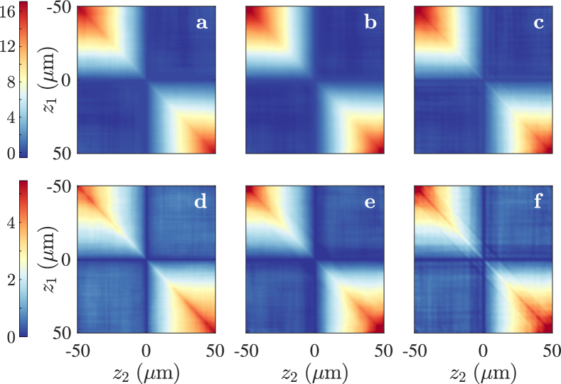
Figure 5: (a) Input second-order correlation $G^{(2)}(z_{1},z_{2})$ for $q=0.5$ (b) TOF reconstruction of $G^{(2)}(z_{1},z_{2})$ with $t=15\;\rm ms$ expansion time (c) Corrected $G^{(2)}(z_{1},z_{2})$ using our analytical formula Eq. (9). The second row (d-f) is the same as the first row (a-c) but with $q=3$. The common phase is sampled from a thermal distribution with $T_{+}=75\;\rm nK$.

Here, we check the validity of our analytical correction Eq. (9) for thermal states by directly correcting the readout phase

$$\phi_{-}^{\rm(corrected)}(z)=\phi_{-}^{\rm(out)}(z)+\Delta\phi_{-}^{\rm(in)}(z)$$ (13)

before computing correlations of the form of Eq. (12). We therefore compute the correction $\Delta\phi_{-}^{\rm(in)}$ directly, assuming knowledge of the input phases. Importantly, we do not linearize the phase correction terms (see Appendix C), as this introduces unphysical higher-order connected correlations for Gaussian states in the corrected phase profiles. We will discuss this below in more detail.

Additionally, due to the multimode nature of thermal states, the perturbative correction $\Delta\phi_{-}^{\rm(in)}$ needs to be low-pass filtered since the correction is only valid for small enough phase gradients, see discussion below Eq. (9). Here we use a hard cutoff $k_{c}$ in momentum space, and fit separate cutoffs for the second and fourth order corrections in order to minimize the squared summed deviation of the full fourth order correlation. Analytically we would expect the cutoff to be such, that $\ell_{t}k_{c}\sim O(1)$, which is in reasonable agreement with the fitted values (see caption of Figs. 6).

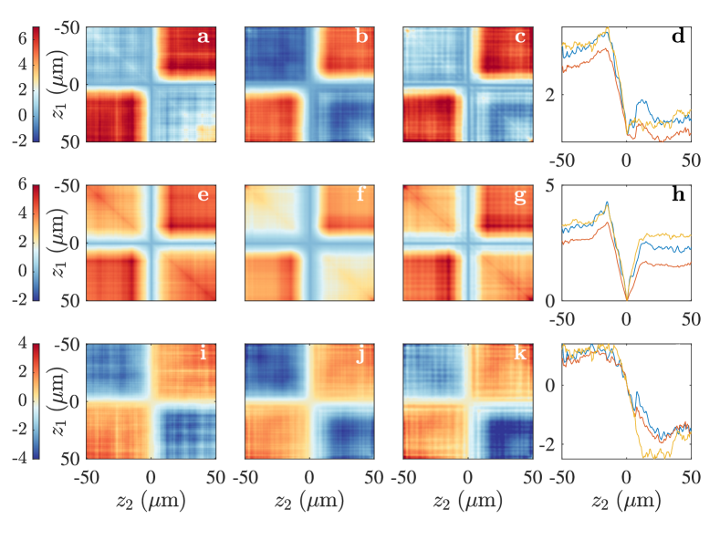
Figure 6: The first row (a-d) shows a cut of the full fourth-order correlation function $G^{(4)}(z_{1},z_{2},z_{3},z_{4})$ with $z_{3}=-z_{4}=15\mu\mathrm{m}$ in the non-Gaussian regime $q=3$. The fitted cutoffs are $k_{c}\simeq 0.6\mu\mathrm{m}^{-1}$ and $k_{c}\simeq 3.1\mu\mathrm{m}^{-1}$ for the second- and fourth-order corrections. Panel (a) shows the input, panel (b) shows TOF reconstruction with $t=15\;\rm ms$, panel (c) shows the corrected reconstruction, and panel (d) shows a cut of $z_{1}=10\;\mu m$ with yellow line showing the input, red line showing the TOF output, and blue line showing the corrected output. Panels (e-h) and panels (i-l) are similar to panels (a-d) but for disconnected correlation $G_{\rm dis}^{(4)}$ and connected correlation $G_{\rm con}^{(4)}$ respectively. The common phase is sampled from a thermal distribution with $T_{+}=75\;\rm nK$.

We first compare the second order correlation $G^{(2)}$ for sine-Gordon Hamiltonian in Gaussian ($q=0.5$) and non-Gaussian ($q=3$) regimes. The comparison is shown in Fig. 5. We observe only small differences between input and output correlation in the small $J$ Gaussian regime of the sine-Gordon model, implying that TOF can faithfully reconstruct Gaussian correlation. However, in non-Gaussian regimes, we observe a spread of cross-shaped strip at the center, which can be interpreted as correction from higher order correlation terms induced by systematic phase shift error. In Figs. 5c-d and Figs. 5g-h, we find that the corrected $G^{(2)}(z_{1},z_{2})$ accurately reproduce the input correlation in both Gaussian and non-Gaussian regimes. This result complements the result in Fig. 3 and demonstrates the validity of our analytical formula Eq. (9) in multimode cases.

Probing non-Gaussianity requires us to probe correlation function of order larger than two. For Gaussian states, the correlation function $G^{(N)}$ factorizes into a function of second-order correlation, such that it only contains disconnected part $G^{N}_{\rm dis}$ while its connected part $G^{N}_{\rm con}$ vanishes. Hence, the approximately Gaussian case of $q=0.5$ is of little interest. In contrast, $G^{N}_{\rm con}$ contains a non-trivial structure for non-Gaussian states. Therefore, in Fig. 6, we compare the input, output, and corrected $G^{(4)}(z_{1},z_{2},z_{3},z_{4})$ cut at fixed $z_{3}=-z_{4}=15\mu m$ in the non-Gaussian regime of $q=3$. We observe that TOF reconstruction introduces a systematic error that modifies the symmetry of the cut, but our correction is able to address the error effectively. Similar corrections can be derived directly for averaged correlations, which do not require explicit knowledge of the single phase profiles but only a well-defined, e.g. thermal, state of the common degrees of freedom. A detailed analysis of the dynamics and mixing of higher-order correlations during TOF reaches beyond the current scope of this paper and will be discussed in detail in a followup publication.

4.2 Full Distribution Functions

Shot-to-shot variations of the interference patterns for pairs of independently created one-dimensional Bose condensates can reveal signatures of quantum fluctuation. In Ref. [13], they show that a key quantity to observe quantum fluctuation in this system is the full distribution function $P(\xi)$ where

$$\xi(l)=\frac{\left|\int_{-l/2}^{l/2}e^{i\phi_{-}(z)}\;dz\right|^{2}}{\left\langle\left|\int_{-l/2}^{l/2}e^{i\phi_{-}(z)}\;dz\right|^{2}\right\rangle},$$ (14)

with $l$ being a variable distance from $0$ to $L$. We are interested in calculating the probability distribution $P(\xi)$ for different length scales $l$. Both theoretically and experimentally, it was observed that for a length scale comparable to the total gas length $\ell\sim L$, the distribution $P(\xi)$ is dominated by thermal fluctuations while for shorter lengths, $P(\xi)$ provides unambiguous signatures of quantum fluctuations [13]. This quantity is also used to study prethermalization of 1D Bose gases after coherent splitting [35, 36, 26].

We compare the input and reconstructed (output) full distribution function $P(\xi)$ for three different length scales in Fig. 7. We find that except for a minor reduction in the high-contrast probability, the qualitative features of the input and output distribution almost coincide. The suppression of the high-contrast probability implies that, as expansion time becomes longer, the medium contrast becomes over-represented and so it could slightly modify the skewness of the underlying distribution. We believe this is due to additional fluctuation coming from the systematic phase shift $\Delta\phi_{-}(z,t)$ which grows with expansion time. Furthermore, by comparing the first and second rows in Fig. 7, we also show that the common phase does not significantly influence the full distribution function. Overall, we observe the same quantum to thermal distribution transition as reported in Ref. [13]. Thus, longitudinal expansion and common phase do not play significant roles here and the existing phase readout protocol can faithfully reproduce the full distribution function function $P(\xi)$.

Figure 7: Full distribution function $P(\xi)$ computed with $10^{3}$ phase profiles sampled from a thermal state with $T_{\pm}=75\;\rm(nK)$. The top (bottom) row a-c (d-f) corresponds to the case where $\phi_{+}(z)=0$ ($\phi_{+}(z)\neq 0$). The length scales are $l=9.8\;\rm{\mu m}$ (a,d), $l=25.5\;\rm\mu m$ (b,e), and $l=49\;\rm\mu m$ (c,f). The blue histogram is the input, red (yellow) histogram is the reconstructed distribution from $7\;\rm ms$ ($15\;\rm ms$) full expansion.

4.3 Velocity-velocity correlation

The spatial derivative of phase has a physical meaning as a velocity field $u_{\pm}(z)=(\hbar/m)\partial_{z}\phi_{\pm}(z)$ in the hydrodynamics description of cold Bosonic gas. Here, we specifically look at the correlation in the relative velocities

$$C_{u}(z,z^{\prime})=\braket{\partial_{z}\phi_{-}(z)\partial_{z^{\prime}}\phi_{-}(z^{\prime})}-\braket{\partial_{z}\phi_{-}(z)}\braket{\partial_{z^{\prime}}\phi_{-}(z^{\prime})},$$ (15)

where $\braket{.}$ denotes average over realization. If the relative velocities of the atoms at $z$ and $z^{\prime}$ are independent, then $C_{u}(z,z^{\prime})$ vanishes. Any non-zero values (discounting statistical fluctuation) for this quantity reflect a correlation in the relative velocities, i.e. if $C_{u}(z,z^{\prime})>0$ the relative velocities of the atoms at $z$ and $z^{\prime}$ tend to align whereas if $C_{u}(z,z^{\prime})<0$ they tend to be opposite. Recently, the velocity-velocity correlation has been measured in experiments to observe curved light cones in a cold-atomic quantum field simulator [19].

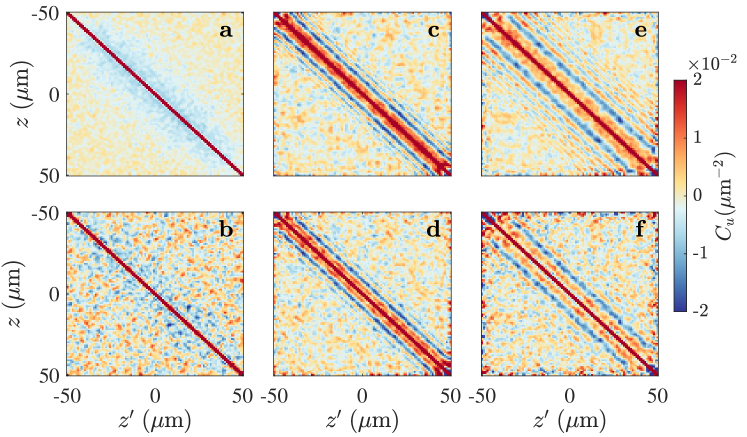
Figure 8: Velocity-velocity correlation $C_{u}(z,z^{\prime})$ calculated from (a) input phase profiles and (b) extracted profiles with $7\rm\;ms$ transversal expansion (c) $7\rm\;ms$ full expansion with $\phi_{+}(z)=0$ and (d) $\phi_{+}(z)\neq 0$. Panels (e)-(f) are the same as (c)-(d) except for $t=15\;\rm ms$. Panel (a) is generated with $10^{4}$ phase profiles whereas panels (b)-(f) are generated with $500$ TOF simulation. The upper bound of the color bar has been adjusted to low values to accentuate structures in the off-diagonals. The input phase profiles are sampled from a thermal distribution with temperatures $T_{\pm}=75\;\rm nK$.

We compare the input and output velocity correlation in Fig. 8. The in situ velocity correlation $C_{u}^{\rm(in)}(z,z^{\prime})$ for a thermal state is not completely diagonal. Instead, it has a weak and short-distance anti-correlation as shown by Fig. 8a.

Interestingly, we observe spatial propagation of the initial anti-correlation in TOF model with longitudinal expansion shown in Figs. 8c-d and Figs. 8e-f, which does not appear in the control simulation with only transversal expansion [Fig. 8b]. We observe the length scale for this correlation (the span of the off-diagonal) increases with a longer expansion time. Such propagation of correlation can be physically understood in a quasi-particle picture, where neighbouring quasi-particles with initial opposite velocity correlation will move further away from each other as the gas expands longitudinally. We also observe alternating patterns of positive and negative correlation which indicates momentum interference in the longitudinal direction [Fig. 8e]. However, this long-distance correlation and anti-correlation are randomized when common phases are involved and only the propagation of the primary anti-correlation persists [Fig. 8f].

This propagation is similar to what has been observed experimentally in the context of a quench from an interacting to non-interacting pair of Luttinger liquids [19]. The difference here is that we report the propagation of velocity correlation due to quenching into a free Hamiltonian induced by TOF measurement protocol. Our results point to the necessity of calibrating the results of dynamical propagation of velocity-velocity correlation such as in Ref. [19] to the measurement background.

4.4 Mean occupation number & temperature

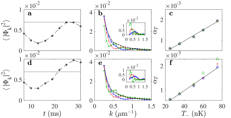
Figure 9: Thermal ($T_{-}=50\;\rm nK$) mean occupation number $\braket{}{\Phi_{k}}{{}^{2}}$ computed using 200 realizations of TOF measurement simulation. In panel a, $k=20\pi/L$ ($\approx 0.63\;\rm\mu m^{-1}$) is fixed but expansion time is varied. In panel b, $k$ is varied but expansion times are fixed at different values: $t=7\;\rm ms$ (blue circles), $t=15\;\rm{ms}$ (red crosses), and $t=30\;\rm ms$ (green triangles). The black solid lines are the ground truths computed from the input data. To emphasize the oscillation in the intermediate mode, we only plot data points with $k\geq 10\pi/L\approx 0.31\;\rm\mu m^{-1}$. The inset shows the residue $\Delta_{k}=\braket{}{\Phi_{k}^{\rm(in)}}{{}^{2}}-\braket{}{\Phi_{k}^{\rm(out)}}{{}^{2}}$. Panel c shows inverse thermal coherence length $\alpha_{T}$ as a function of temperature $T_{-}$. Panels d-f are the repetition of a-c but include common phase with temperature $T_{+}=T_{-}$.

The mean power spectrum $\braket{}{\Phi_{k}}{{}^{2}}$ where $\Phi_{k}=(1/L)\int_{-L/2}^{L/2}e^{-ikz}\phi_{-}(z)\;dz$ is another relevant physical quantity of the gas, since it is related to the gas temperature $T$. In particular, it is directly related to the temperature of the relative sector $T_{-}$, which in general can be different from the temperature of the common sector $T_{+}$. For a uniform thermal state, their relation is given by [37]

$$\braket{}{\Phi_{k}}{{}^{2}}=\frac{mk_{B}T}{\hbar^{2}k^{2}n_{\rm 1D}}=\frac{\alpha_{T}}{k^{2}},$$ (16)

where $\alpha_{T}=1/\lambda_{T}=mk_{B}T/(\hbar^{2}n_{\rm 1D})$ is inverse thermal coherence length. By fitting the mean power spectrum with respect to $k^{-2}$, we can obtain $\alpha_{T}$ and extract the temperature of the relative phase $T_{-}$. For the purpose of our simulation, we will assume the relative and common degrees of freedom are in thermal equilibrium with respect to each other ($T_{+}=T_{-}$).

We start by comparing the input and output mean power spectrum for a thermal state with a fixed temperature $T_{-}=50\;\rm nK$. We first fixed the momentum to be $k=20\pi/L$ and varied the expansion time $t$. We find a non-trivial oscillation of $\braket{}{\Phi_{k}^{\rm(out)}}{{}^{2}}$ with respect to $t$ attributed to longitudinal expansion [Figs. 9a,d]. In principle, a perfectly faithful reconstruction of $\braket{}{\Phi_{k}}{{}^{2}}$ generally should not depend on the expansion time.

This oscillation is also visible when we plot $\braket{}{\Phi_{k}}{{}^{2}}$ as a function of $k$ for different values of expansion time as shown in Figs. 9b,e, where we have omitted the low-momentum population $k<10\pi/L$ to emphasize the oscillation in the intermediate mode regime. The insets in Figs. 9b,e show the residue between input and output power spectrum $\Delta_{k}=\braket{}{\Phi_{k}^{\rm(in)}}{{}^{2}}-\braket{}{\Phi_{k}^{\rm{(out)}}}{{}^{2}}$, which qualitatively resembles the evolution of density ripple spectrum [20]. As expansion time gets longer, the maximum of the residue $\Delta_{k}^{(\max)}=\max_{k}(\Delta_{k})$ grows and its peak location $k_{\max}$ shifts to a lower mode.

Free expansion dynamics has no mode-mode interaction so the origin of the oscillation must be due to single-mode dynamics. We hypothesize that such an oscillation arises from single-mode free particle quadrature dynamics between phase fluctuation and density fluctuation which has a characteristic frequency $\hbar k^{2}/2m$. As a result, energy goes back and forth between phase and density fluctuations of a single mode. However, since density fluctuation is ignored in our analysis, only one of the quadrature fluctuations is included in Fig. 9. The energy in phase quadrature can not exceed its initial energy. This may explain why the output power spectrum appears to be upper-bounded by its in situ values [Figs. 9a,b]. However, this upper bound can be violated for high enough common phase temperature [Figs. 9d,e] because initial common phase fluctuation can give extra energy to the relative phase [see Eq. (9)].

Finally, we check the impact of this oscillation to the reading of temperature using Eq. (16). We perform fitting $\braket{}{\Phi_{k}}{{}^{2}}=\alpha_{T}k^{-2}$ for different values of $T_{-}$ and then plot $\alpha_{T}$ as a function of $T_{-}$ shown in Figs. 9c,f. We find that the oscillation due to longitudinal expansion does not significantly affect the readout of temperatures, but the additional fluctuation from common phase does make a difference for medium to long expansion time ($t>15\;\rm ms$) and high enough $T_{+}\geq 60\;\rm nK$.

5 Summary & Discussion

In summary, we derived an analytical expression for systematic phase shift error due to longitudinal expansion, specifically due to mixing with the common degrees of freedom and the presence of longitudinal Green’s function. We also assessed the error propagation into the reconstruction of physical quantities related to the statistics of relative phase field.

The analysis done in this paper is subjected to the validity of the modelling approximations [see Fig. 1]. One approximation we made was to ignore the broadening due to atomic repulsion $\sigma_{0}^{2}(z)=\sigma_{0}^{2}\sqrt{1+2a_{s}n_{0}(z)}\approx\sigma_{0}^{2}$. Relaxing this assumption makes it difficult to obtain an analytical relation between the initial state and the final measured density due to the non-separability of the initial state. However, assuming that the non-separability is weak, there exists an ansatz that can phenomenologically capture the most relevant features of interference image broadened by scattering. The ansatz [22] is to replace all $\sigma_{0}$ appearing in Eq. (4) by the broadened $\sigma_{0}(z)$. Note that the fringe spacing now also depends on $z$, i.e. $k(z,t)=d/(\sigma_{0}^{2}(z)\omega t)$. Taking longitudinal expansion into account, we can develop a similar ansatz to modify Eq. (5). We replace all $\sigma_{0}$ with $\sigma_{0}(z^{\prime})$ and propagate it with a Green’s function. Preliminary numerical simulation with this ansatz has revealed that scattering only affects the width of the final image, but it does not significantly affect other extracted fit parameters [Fig. 10 in Appendix E].

Furtheremore, throughout this paper, we have ignored the impact of density fluctuations by assuming $\delta n_{1,2}\ll n_{0}$ which might not be accurate in higher temperatures. Moreover, we have ignored the final state interaction in our analysis so that the time evolution is fully ballistic. A more refined modelling would be to include the hydrodynamic effect at the initial phase of the expansion, where interaction energy still remains in the system. Only after interaction energy sufficiently decays, does the system follow fully ballistic dynamics. In future work, we will explore the role of final state interaction with a 3D Gross-Pitaevskii equation.

In addition to refining the model, another future direction is to extract the common phase from TOF interference pattern. From this study, we find that information about the common phase is imprinted on the density ripple. Density ripple has been used for thermometry in the case of single condensate [20, 10]. However, the significance of density ripple in the two condensates case has not been explored. Developing a readout method of the common phase from density ripple could be useful in unlocking the full potential of 1D Bose gas interference experiments, especially in non-equilibrium. For example, it is known that the higher order correction to the sine-Gordon model for describing tunnel-coupled 1D Bose gas involves a coupling between relative and common phase [38, 24]. Moreover, density imbalances between atoms in the two double wells can also lead to coupling between relative and common phases, leading to double-light cone thermalization [29]. Finally, having access to a common phase could also allow us to simulate spin-charge transport in 1D Bose gases [29, 36]. This work serves as a fundamental starting point for further research in this direction.

In conclusion, our quantitative analysis confirms the reliability of time-of-flight measurements within defined parameters. Additionally, our study underscores two significant findings. Firstly, it identifies avenues for enhancing modelling methods to achieve more accurate reconstructions. Secondly, we observe the potential for extracting additional information from TOF measurements[39], thus augmenting the measurement capabilities of cold atomic quantum simulators. These advancements may serve to enhance future explorations of the physics of cold atomic systems.

6 Acknowledgments

We would like to thank Yuri van Nieuwkerk for discussions at the early stages of this work and Amin Tajik for help in using imaging resolution modelling developed by Thomas Schweigler and Frederik Moller.

TM, MG, KZA and NN were supported through the start-up grant of the Nanyang Assistant Professorship of Nanyang Technological University, Singapore which was awarded to NN. Additionally, MG has been supported by the Presidential Postdoctoral Fellowship of the Nanyang Technological University. SE acknowledges support by the Austrian Science Fund (FWF) [Grant No. I6276, QuFT-Lab].

Appendix A Free expansion dynamics

In this Appendix, we will derive the expansion dynamics of the Bosonic fields including both transversal and longitudinal dynamics, elucidating earlier works by Yuri, Essler, and Schmiedmayer [21]. Let us consider the 3D time-dependent Gross-Pitaevskii equation

$$i\hbar\frac{\partial\Psi}{\partial t}=-\frac{\hbar^{2}}{2m}\nabla^{2}\Psi+V(x,y,z)\Psi+g|\Psi|^{2}\Psi.$$ (17)

Upon free expansion, we set all trapping potential to zero $V(x,y,z)=0$ and we neglect final state interaction $g=0$, so that the equation of motion is essentially that of free particles. Then, the time evolution is given by convolution with a Green’s function

$$\Psi(\vec{r},z,t)=\int d^{2}\vec{r}^{\prime}\;dz\;G(\vec{r}-\vec{r}^{\prime},t)G(z-z^{\prime},t)\Psi(\vec{r}^{\prime},z,0),$$ (18)

where we have separated the transversal $\vec{r}=(x,y)$ and longitudinal $z$ components of the evolution and that $G(\xi,t)=\sqrt{m/2\pi i\hbar t}\exp(-m\xi^{2}/2i\hbar t)$ is the free, single-particle Green’s function.

Next, we substitute the initial state [Eq. (1) in the main text] and integrate over the transverse directions, giving us the time-evolved fields

$$\Psi_{1,2}(x,y,z,t)= \frac{1}{\sqrt{\pi\sigma_{t}^{2}}}\exp\left(-\frac{(x\pm d/2)^{2}+y^{2}}{2\sigma_{t}^{2}}\right)\exp\left(\frac{im[(x\pm d/2)^{2}+y^{2}]}{2\hbar t}\right)\times$$

$$\int dz^{\prime}\;G(z-z^{\prime},t)\sqrt{n_{0}(z^{\prime})}e^{i\phi_{1,2}(z^{\prime})},$$ (19)

where $\sigma_{t}=\sigma_{0}\sqrt{1+\omega^{2}t^{2}}$ is the expanded width. Note that we have assumed $\omega t\gg 1$ and explicitly ignored density fluctuation $\delta n_{1,2}\ll n_{0}$.

We are concerned with the coherent superposition of the two fields when they overlap

$$\Psi(\vec{r},z,t)=\Psi_{1}(\vec{r},z,t)+\Psi_{2}(\vec{r},z,t).$$ (20)

If we wait long enough such that $d\ll\sigma_{t}$ the transverse Gaussian envelopes can be approximated into a single Gaussian centred at the origin. Consequently, the expression for the superposed field becomes relatively simple

$$\Psi(\vec{r},z,t)=Ae^{-\frac{|\vec{r}|^{2}}{\sigma_{t}^{2}}}\int_{-L/2}^{L/2}dz^{\prime}\;G(z-z^{\prime},t)\sqrt{n_{0}(z^{\prime})}e^{i\phi_{+}(z^{\prime})/2}\cos\left(\frac{kx+\phi_{-}(z^{\prime})}{2}\right).$$ (21)

with $A$ being a normalization constant, $k=md/(\hbar t)$ is the inverse fringe spacing, $\phi_{\mp}(z)=\phi_{2}(z)\mp\phi_{1}(z)$ are relative (-) and common (+) phases. Equation (5) in the main text is then easily obtained from $\rho_{\text{TOF}}(x,z,t)=\int dy\;|\Psi(\vec{r},z,t)|^{2}$.

Appendix B Derivation of the transverse fit formula

We continue to derive the transversal fit formula [Eq. (4) in the main text] including the effects of mean density imbalance as well as density fluctuations. This section is a restatement of other similar derivations in the literature [23, 22, 21].

We start from the extended version of Eq. (4) in the main text, taking into account density fluctuations and different mean densities in each well

$$\rho_{\rm TOF}(x,z,t)=Ae^{-x^{2}/\sigma_{t}^{2}}\bigg{|}\int_{-L/2}^{L/2} dz^{\prime}G(z^{\prime}-z,t)e^{i\phi_{+}(z^{\prime})/2}\Big{[}\sqrt{n_{1}(z^{\prime})+\delta n_{1}(z^{\prime})}e^{-i\phi_{-}(z^{\prime})/2}e^{-ikx/2}$$

$$+\sqrt{n_{2}(z^{\prime})+\delta n_{2}(z^{\prime})}e^{i\phi_{-}(z^{\prime})/2}e^{ikx/2}\Big{]}\bigg{|}^{2}.$$ (22)

Next, we ignore longitudinal dynamics by substituting $G(z-z^{\prime},t)\rightarrow\delta(z-z^{\prime})$ and integrate over $z^{\prime}$

$$\rho_{\rm TOF}^{\perp}(x,z,t) =Ae^{-x^{2}/\sigma_{t}^{2}}\Bigg{|}\sqrt{n_{1}(z)+\delta n_{1}(z)}e^{-i\frac{kx+\phi_{-}(z)}{2}}+\sqrt{n_{2}(z)+\delta n_{2}(z)}e^{i\frac{kx+\phi_{-}(z)}{2}}\Bigg{|}^{2}$$

$$\cong Ae^{-x^{2}/\sigma_{t}^{2}}\left[n_{+}(z)+\delta n_{+}(z)\right]\left[1+C(z)\cos(kx+\phi_{-}(z)\right],$$ (23)

where

$$n_{+}(z)=n_{1}(z)+n_{2}(z)\qquad\delta n_{+}(z)=\delta n_{1}(z)+\delta n_{2}(z),$$ (24)

and interference contrast $C(z)$

$$C(z)=\frac{2\sqrt{(n_{1}(z)+\delta n_{1}(z))(n_{2}(z)+\delta n_{2}(z))}}{n_{+}(z)+\delta n_{+}(z)}.$$ (25)

Note that contrast is maximum $C(z)=1$ when $n_{1}(z)=n_{2}(z)$ and $\delta n_{1}(z)=\delta n_{2}(z)=0$. After absorbing $n_{+}(z),\delta n_{+}(z)$ into the normalization constant $A$, we recover Eq. (4) in the main text.

Appendix C Corrections due to longitudinal dynamics

Here, we present a detailed derivation of the new analytical results contained in the main text [Eqs. (7) - (9)]. We start from the full expansion formula [Eq. (5) in the main text]

$$\rho_{\text{TOF}}(x,z,t)=A(t)e^{-x^{2}/\sigma_{t}^{2}}\;\Bigg{|}\int_{-L/2}^{L/2}dz^{\prime}G(z-z^{\prime},t)I(x,z^{\prime},t)\Bigg{|}^{2},$$ (26)

where

$$I(x,z^{\prime},t)=\sqrt{n_{0}(z^{\prime})}e^{i\phi_{+}(z^{\prime})/2}\cos\Bigg{(}\frac{kx+\phi_{-}(z^{\prime})}{2}\Bigg{)}.$$ (27)

We treat longitudinal expansion perturbatively by performing Taylor expansion of $I(x,z^{\prime},t)$ around small $\Delta z=z^{\prime}-z$

$$I(x,z^{\prime},t)=I(x,z,t)+\Delta z\;\partial_{z}I+\frac{\Delta z^{2}}{2}\partial_{z}^{2}I+O\big{(}\Delta z^{3}\big{)}.$$ (28)

Substituting Eq. (28) to the integral in Eq. (26), we find that the zeroth order term will give us the transversal expansion formula with a maximum contrast $C=1$

$$\rho_{\rm TOF}^{\perp}(x,z,t) \approx A(t)e^{-x^{2}/\sigma_{t}^{2}}\Big{|}I(x,z,t)\int_{-\infty}^{\infty}G(\Delta z,t)\;d(\Delta z)\Big{|}^{2}$$

$$=\frac{A(t)n_{0}(z)}{2}e^{-x^{2}/\sigma_{t}^{2}}[1+\cos\big{(}kx+\phi_{-}(z)\big{)}],$$ (29)

where we have extended the integration limit from $[-L/2,L/2]$ to $(-\infty,\infty)$.

Let us now compute the higher-order corrections. The first order term will vanish because it is proportional to $\int_{-\infty}^{\infty}\bigl{(}\Delta z\;G(\Delta z,t)\bigr{)}\;d(\Delta z)=0$. Therefore, the next non-zero correction will come from the second-order term,

$$\rho_{\rm TOF}(x,z,t)\approx A(t)e^{-x^{2}/\sigma_{t}^{2}}\Big{|}I+\frac{\partial_{z}^{2}I}{2}\int_{-\infty}^{\infty}\bigl{(}\Delta z^{2}G(\Delta z,t)\bigr{)}\;d(\Delta z)\Big{|}^{2}.$$ (30)

It is easy to check that $\int_{-\infty}^{\infty}\bigl{(}\Delta z^{2}G(\Delta z,t)\bigr{)}d(\Delta z)=\frac{i\hbar t}{m}=i\ell_{t}^{2}$ where we have defined $\ell_{t}=\sqrt{\hbar t/m}$ to be the length scale of longitudinal expansion. Substituting the integral and defining a derivative with respect to scaled coordinate $\eta=z/\ell_{t}$, one obtains

$$\rho_{\rm TOF}(x,z,t) \approx A(t)e^{-x^{2}/\sigma_{t}^{2}}\Big{|}I+\frac{1}{2}i\;\partial_{\eta}^{2}I\Big{|}^{2}$$ (31)

$$=\rho_{\rm TOF}^{\perp}(x,z,t)+A(t)e^{-x^{2}/\sigma_{t}^{2}}\Big{[}-\text{Im}(I^{*}\partial_{\eta}^{2}I)+\frac{1}{4}|\partial_{\eta}^{2}I|^{2}\Big{]}$$ (32)

$$=\rho_{\text{TOF}}^{\perp}(x,z,t)+\Delta\rho^{(2)}+\Delta\rho^{(4)}$$ (33)

with $\Delta\rho^{(n)}$ being the n-th order correction terms in scaled derivatives $\partial_{\eta}I$ which we expect to be small [see the main text for reasoning].

We first focus on the leading order correction $\Delta\rho^{(2)}=-A(t)e^{-x^{2}/\sigma_{t}^{2}}\text{Im}(I^{*}\partial_{\eta}^{2}I).$ To compute this term, we must first compute $\partial_{z}^{2}I=\ell_{t}^{-2}\partial_{\eta}^{2}I$

$$\partial_{z}^{2}I=\Gamma(z)\cos\left(\frac{kx+\phi_{-}(z)}{2}\right)-\Lambda(z)\sin\left(\frac{kx+\phi_{-}(z)}{2}\right),$$ (34)

where

$$\Gamma(z)=\partial_{z}^{2}\psi_{+}-\frac{\psi_{+}(\partial_{z}\phi_{-})^{2}}{4}\qquad\Lambda(z)=\partial_{z}\psi_{+}\partial_{z}\phi_{-}+\frac{\psi_{+}\partial_{z}^{2}\phi_{-}}{2}$$ (35)

and $\psi_{+}(z)=\sqrt{n_{0}(z)}e^{i\phi_{+}(z)/2}$. For simplicity, we will consider the case $n_{0}(z)=n_{1D}=\text{const.}$ which gives us

$$\Delta\rho^{(2)}=-A(t)e^{-x^{2}/\sigma_{t}^{2}}\frac{n_{0}}{4}[\partial_{\eta}^{2}\phi_{+}(1+\cos(kx+\phi_{-}))-\partial_{\eta}\phi_{-}\partial_{\eta}\phi_{+}\sin(kx+\phi_{-})]\ .$$ (36)

Combining the above with the expression for $\rho_{\rm TOF}^{\perp}$ in Eq. (C) and using trigonometric identity $a\cos x+b\sin x=\sqrt{a^{2}+b^{2}}\cos(x-\alpha)$ with $\tan\alpha=b/a$ we can express $\rho_{\rm TOF}$ as

$$\rho_{\rm TOF}(x,z,t)\approx A^{\prime}(z,t)e^{-x^{2}/\sigma_{t}^{2}}[1+C(z,t)\cos(kx+\phi_{-}(z)-\Delta\phi_{-}^{(2)}(z,t))]$$ (37)

with

$$A^{\prime}(z,t)=\frac{A(t)n_{0}(z)}{2}\left(1-\frac{1}{2}\partial_{\eta}^{2}\phi_{+}\right)\qquad$$ (38)

$$C(z,t)=\sqrt{\left(1-\frac{1}{2}\partial_{\eta}^{2}\phi_{+}\right)^{2}+\left(\frac{1}{2}\partial_{\eta}\phi_{-}\partial_{\eta}\phi_{+}\right)^{2}}$$ (39)

$$\Delta\phi_{-}^{(2)}(z,t)=\arctan\left(\frac{\frac{1}{2}\partial_{\eta}\phi_{+}\partial_{\eta}\phi_{-}}{1-\frac{1}{2}\partial_{\eta}^{2}\phi_{+}}\right)\approx\frac{1}{2}\partial_{\eta}\phi_{+}\partial_{\eta}\phi_{-}\ .$$ (40)

In the main text, we are also interested in cases where $\phi_{+}=0$. For such cases, the above derivation implies $\Delta\phi_{-}^{(2)}=0$ and so higher order terms need to be taken into account.

Let us now consider the $\Delta\rho^{(4)}$ term in Eq. (31). Below, we explicitly write the form of $|\partial_{z}^{2}I|^{2}$,

$$|\partial_{z}^{2}I|^{2}= \frac{1}{2}\Big{(}|\Gamma(z)|^{2}+|\Lambda(z)|^{2}\Big{)}+\frac{1}{2}\Big{(}|\Gamma(z)|^{2}-|\Lambda(z)|^{2}\Big{)}\cos(kx+\phi_{-}(z))$$

$$-\text{Re}\Big{(}\Gamma^{*}(z)\Lambda(z)\Big{)}\sin(kx+\phi_{-}(z)).$$ (41)

To simplify the expressions, we again use the assumption $n_{0}=n_{\rm 1D}=\text{const.}$, such that

$$\Gamma(z)=\frac{\sqrt{n_{\rm 1D}}}{2{\ell_{t}^{2}}}e^{i\phi_{+}(z)/2}F(\eta)\qquad\Lambda(z)=\frac{\sqrt{n_{\rm 1D}}}{2{\ell_{t}^{2}}}e^{i\phi_{+}(z)/2}G(\eta),$$ (42)

where $F(\eta),\;G(\eta)$ are dimensionless functions

$$F(\eta)=\partial_{\eta}^{2}\phi_{+}-\frac{(\partial_{\eta}\phi_{+})^{2}+(\partial_{\eta}\phi_{-})^{2}}{2}\qquad G(\eta)=i(\partial_{\eta}\phi_{+})(\partial_{\eta}\phi_{-})+\partial_{\eta}^{2}\phi_{-}.$$ (43)

Thus, the density correction is given by,

$$\Delta\rho^{(4)}=\frac{1}{16}A(t)e^{-x^{2}/\sigma_{t}^{2}}(|F|^{2}+|G|^{2})\bigg{[}1+\frac{|F|^{2}-|G|^{2}}{|F|^{2}+|G|^{2}}\cos(kx+\phi_{-})-\frac{{2}\text{Re}(F^{*}G)}{|F|^{2}+|G|^{2}}\sin(kx+\phi_{-})\bigg{]}.$$ (44)

Putting $\rho_{\text{TOF}}^{\perp},\;\Delta\rho^{(2)}$, and $\Delta\rho^{(4)}$ together, one can always recast the entire expression into the form

$$\rho_{\rm TOF}(x,z,t)\approx A(z,t)e^{-x^{2}/\sigma_{t}^{2}}\left[1+C(z,t)\cos\big{(}kx+\phi_{-}(z)-\Delta\phi_{-}(z)\big{)}\right],$$ (45)

which is one of the main analytical results of the main text [Eq. (7)]. Note that the validity of Eq. (45) does not depend on the specific forms of $A(z,t)$ and $C(z,t)$. It only relies on the fact that the correction terms are always proportional to $\sin(kx+\phi_{-})$ or $\cos(kx+\phi_{-})$ and so it will also be valid in varying mean density cases.

In the simplest case of $n_{0}(z)=n_{\rm 1D}$ and $\phi_{+}(z)=0$, we find a higher order phase shift

$$\Delta\phi_{-}^{(4)}(z,t)\Big{|}_{\phi_{+}=0}=-\arctan\Bigg{(}\frac{2\text{Re}(F^{*}G)}{8+(|F|^{2}-|G|^{2})}\Bigg{)}\approx\frac{1}{8}\left(\partial_{\eta}\phi_{-}\right)^{2}\left(\partial_{\eta}^{2}\phi_{-}\right).$$ (46)

Summing Eq. (40) with Eq. (46) gives another analytical result of the main text [Eq. (9)].

Appendix D Relative phase fitting initialization

In this section, we show the approximate linear relationship between relative phase $\phi_{-}$ and the interference peak’s transversal position $x_{\rm max}$ for a fixed longitudinal position $z$. We use this approximate linear relationship to provide an initial guess for the optimizer used in fitting.

For simplicity, we assume $\rho_{\rm TOF}$ to be well approximated by the standard fitting formula [Eq. (4) in the main text] with $C=1$. To find the transversal peak location, we simply solve $\partial\rho_{\rm TOF}^{\perp}/\partial x|_{x=x_{\text{max}}}=0$, which gives the condition

$$\frac{2x}{\sigma_{t}^{2}}\bigg{[}1+\cos\left(kx_{\rm max}+\phi_{-}^{(0)}\right)\bigg{]}+k\sin\left(kx_{\rm max}+\phi_{-}^{(0)}\right)=0,$$ (47)

where the superscript 0 indicates a ’guess’ value (initial value to feed into the optimizer). Using the half-angle formula, we obtain

$$\cos\left(\frac{kx_{\rm max}+\phi_{-}^{(0)}}{2}\right)\Bigg{[}\frac{2x}{\sigma_{t}^{2}}\cos\Bigg{(}\frac{kx_{\rm max}+\phi_{-}^{(0)}}{2}\Bigg{)}+k\sin\Bigg{(}\frac{kx_{\rm max}+\phi_{-}^{(0)}}{2}\Bigg{)}\Bigg{]}=0,$$ (48)

For non-zero interference, we must have $\cos([kx+\phi_{-}^{(0)}]/2)\neq 0$ and so to satisfy Eq. (48), the terms inside the paranthesis have to vanish. Finally, we can solve for $\phi_{-}^{(0)}$ and the result is

$$\phi_{-}^{(g)}=-kx_{\text{max}}+2\arctan\Big{(}-\frac{2\omega t}{1+\omega^{2}t^{2}}\frac{x_{\rm max}}{d}\Big{)}\approx-\frac{md}{\hbar t}x_{\rm max}$$ (49)

where in the last approximation we have used $\omega t\gg 1$ such that the $\arctan$ function changes very slowly with $x_{\rm max}$.

Appendix E Additional plots

Figure 10: Single shot relative phase extraction with and without scattering-induced broadening. Panels a - b show interference pattern without ($\sigma_{0}=\text{const.}$) and with scattering-induced broadening ($\sigma_{0}^{2}(z)=\sigma_{0}^{2}\sqrt{1+a_{s}n_{0}(z)}$). Panels c-f show the extracted fit parameters $\{\phi_{-},A,C,\sigma\}$ without (red) and with interaction broadening. The black solid (dashed) line in panel c is the input relative (common) phase. From this figure, we observe that scattering-induced broadening does not significantly impact the extracted fit parameters except the width.

References

- [1] A. D. Cronin, J. Schmiedmayer and D. E. Pritchard, Optics and interferometry with atoms and molecules, Rev. Mod. Phys. 81(3), 1051 (2009).
- [2] T. Langen, R. Geiger and J. Schmiedmayer, Ultracold atoms out of equilibrium, Annu. Rev. Cond. Mat. Phys. 6, 201 (2015).
- [3] S. Hofferberth, I. Lesanovsky, B. Fischer, T. Schumm and J. Schmiedmayer, Non-equilibrium coherence dynamics in one-dimensional bose gases, Nature 449, 324 (2007).
- [4] T. Langen, R. Geiger, M. Kuhnert, B. Rauer and J. Schmiedmayer, Local emergence of thermal correlations in an isolated quantum many-body system, Nature Phys. 9, 640 (2013), 10.1038/nphys2739.
- [5] T. Langen, S. Erne, R. Geiger, B. Rauer, T. Schweigler, M. Kuhnert, W. Rohringer, I. E. Mazets, T. Gasenzer and J. Schmiedmayer, Experimental observation of a generalized Gibbs ensemble, Science 348, 207 (2015), 10.1126/science.1257026.
- [6] M. Tajik, I. Kukuljan, S. Sotiriadis, B. Rauer, T. Schweigler, F. Cataldini, J. Sabino, F. Møller, P. Schüttelkopf, S.-C. Ji et al., Verification of the area law of mutual information in a quantum field simulator, Nature Physics pp. 1–5 (2023).
- [7] M. Gluza, J. Sabino, N. H. Ng, G. Vitagliano, M. Pezzutto, Y. Omar, I. Mazets, M. Huber, J. Schmiedmayer and J. Eisert, Quantum field thermal machines, PRX Quantum 2(3), 030310 (2021).
- [8] J. Schmiedmayer, One-dimensional atomic superfluids as a model system for quantum thermodynamics, In Thermodynamics in the Quantum Regime: Fundamental Aspects and New Directions, pp. 823–851. Springer (2019).
- [9] A. Imambekov, V. Gritsev and E. Demler, Ultracold Fermi gases, Proc. Internat. School Phys. Enrico Fermi, 2006, chap. Fundamental noise in matter interferometers, IOS Press, Amsterdam, The Netherlands (2007).
- [10] F. Møller, T. Schweigler, M. Tajik, J. a. Sabino, F. Cataldini, S.-C. Ji and J. Schmiedmayer, Thermometry of one-dimensional bose gases with neural networks, Phys. Rev. A 104, 043305 (2021), 10.1103/PhysRevA.104.043305.
- [11] M. Pigneur, T. Berrada, M. Bonneau, T. Schumm, E. Demler and J. Schmiedmayer, Relaxation to a phase-locked equilibrium state in a one-dimensional bosonic josephson junction, Phys. Rev. Lett. 120 (2018), 10.1103/physrevlett.120.173601.
- [12] M. Gluza, T. Schweigler, M. Tajik, J. Sabino, F. Cataldini, F. S. Møller, S.-C. Ji, B. Rauer, J. Schmiedmayer, J. Eisert and S. Sotiriadis, Mechanisms for the emergence of Gaussian correlations, SciPost Phys. 12, 113 (2022), 10.21468/SciPostPhys.12.3.113.
- [13] S. Hofferberth, I. Lesanovsky, T. Schumm, A. Imambekov, V. Gritsev, E. Demler and J. Schmiedmayer, Probing quantum and thermal noise in an interacting many-body system, Nature Physics 4(6), 489 (2008).
- [14] T. Kitagawa, A. Imambekov, J. Schmiedmayer and E. Demler, The dynamics and prethermalization of one-dimensional quantum systems probed through the full distributions of quantum noise, New J. Phys. 13(7), 073018 (2011), 10.1088/1367-2630/13/7/073018.
- [15] M. Gluza, T. Schweigler, B. Rauer, C. Krumnow, J. Schmiedmayer and J. Eisert, Quantum read-out for cold atomic quantum simulators, Comm. Phys. 3, 12 (2020), 10.1038/s42005-019-0273-y.
- [16] T. Schweigler, V. Kasper, S. Erne, I. Mazets, B. Rauer, F. Cataldini, T. Langen, T. Gasenzer, J. Berges and J. Schmiedmayer, Experimental characterization of a quantum many-body system via higher-order correlations, Nature 545, 323 (2017).
- [17] T. V. Zache, T. Schweigler, S. Erne, J. Schmiedmayer and J. Berges, Extracting the field theory description of a quantum many-body system from experimental data, Phys. Rev. X 10, 011020 (2020), 10.1103/PhysRevX.10.011020.
- [18] T. Langen, R. Geiger, M. Kuhnert, B. Rauer and J. Schmiedmayer, Local emergence of thermal correlations in an isolated quantum many-body system, Nature Phys. 9, 640 (2013).
- [19] M. Tajik, M. Gluza, N. Sebe, P. Schüttelkopf, F. Cataldini, J. Sabino, F. Møller, S.-C. Ji, S. Erne, G. Guarnieri et al., Experimental observation of curved light-cones in a quantum field simulator, Proceedings of the National Academy of Sciences 120(21), e2301287120 (2023).
- [20] A. Imambekov, I. E. Mazets, D. S. Petrov, V. Gritsev, S. Manz, S. Hofferberth, T. Schumm, E. Demler and J. Schmiedmayer, Density ripples in expanding low-dimensional gases as a probe of correlations, Phys. Rev. A 80, 033604 (2009), 10.1103/PhysRevA.80.033604.
- [21] Y. D. van Nieuwkerk, J. Schmiedmayer and F. Essler, Projective phase measurements in one-dimensional Bose gases, SciPost Physics 5, 046 (2018), 10.21468/scipostphys.5.5.046.
- [22] T. Schweigler, Correlations and dynamics of tunnel-coupled one-dimensional Bose gases, Ph.D. thesis, TU Wien, arxiv:1908.00422 (2019).
- [23] T. Langen, Non-equilibrium dynamics of one-dimensional Bose gases, Springer (2015).
- [24] Y. D. van Nieuwkerk, J. Schmiedmayer and F. H. Essler, Josephson oscillations in split one-dimensional bose gases, arXiv preprint arXiv:2010.11214 (2020).
- [25] J.-F. Mennemann, S. Erne, I. Mazets and N. J. Mauser, The discrete green’s function method for wave packet expansion via the free schrödinger equation, arXiv preprint arXiv:2303.09464 (2023).
- [26] D. A. Smith, M. Gring, T. Langen, M. Kuhnert, B. Rauer, R. Geiger, T. Kitagawa, I. Mazets, E. Demler and J. Schmiedmayer, Prethermalization revealed by the relaxation dynamics of full distribution functions, New Journal of Physics 15(7), 075011 (2013).
- [27] M. Rigol, V. Dunjko, V. Yurovsky and M. Olshanii, Relaxation in a completely integrable many-body quantum system: An ab initio study of the dynamics of the highly excited states of 1D lattice hard-core bosons, Phys. Rev. Lett. 98, 050405 (2007), 10.1103/PhysRevLett.98.050405.
- [28] L. Salasnich, A. Parola and L. Reatto, Transition from three dimensions to one dimension in bose gases at zero temperature, Phys. Rev. A 70, 013606 (2004), 10.1103/PhysRevA.70.013606.
- [29] T. Langen, T. Schweigler, E. Demler and J. Schmiedmayer, Double light-cone dynamics establish thermal states in integrable 1d bose gases, New Journal of Physics 20(2), 023034 (2018).
- [30] C. M. Bender and S. A. Orszag, Advanced mathematical methods for scientists and engineers I: Asymptotic methods and perturbation theory, Springer Science & Business Media (2013).
- [31] C. Mora and Y. Castin, Extension of Bogoliubov theory to quasicondensates, Phys. Rev. A 67, 053615 (2003), 10.1103/PhysRevA.67.053615.
- [32] T. Schweigler, V. Kasper, S. Erne, I. E. Mazets, B. Rauer, F. Cataldini, T. Langen, T. Gasenzer, J. Berges and J. Schmiedmayer, Experimental characterization of a quantum many-body system via higher-order correlations, Nature 545(7654), 323 (2017), 10.1038/nature22310.
- [33] S. Beck, I. E. Mazets and T. Schweigler, Nonperturbative method to compute thermal correlations in one-dimensional systems, Phys. Rev. A 98, 023613 (2018), 10.1103/PhysRevA.98.023613.
- [34] C. W. Gardiner et al., Handbook of stochastic methods, vol. 3, springer Berlin (1985).
- [35] M. Gring, M. Kuhnert, T. Langen, T. Kitagawa, B. Rauer, M. Schreitl, I. E. Mazets, D. A. Smith, E. Demler and J. Schmiedmayer, Relaxation and prethermalization in an isolated quantum system, Science 337, 1318 (2012).
- [36] T. Kitagawa, A. Imambekov, J. Schmiedmayer and E. Demler, The dynamics and prethermalization of one-dimensional quantum systems probed through the full distributions of quantum noise, New Journal of Physics 13(7), 073018 (2011).
- [37] H.-P. Stimming, N. J. Mauser, J. Schmiedmayer and I. Mazets, Fluctuations and stochastic processes in one-dimensional many-body quantum systems, Phys. Rev. Lett. 105(1), 015301 (2010), 10.1103/PhysRevLett.105.015301.
- [38] V. Gritsev, A. Polkovnikov and E. Demler, Linear response theory for a pair of coupled one-dimensional condensates of interacting atoms, Phys. Rev. B 75, 174511 (2007), 10.1103/PhysRevB.75.174511.
- [39] T. Murtadho, M. Gluza and N. Ng (2024), In preparation.