Anomalous Hall Crystals in Rhombohedral Multilayer Graphene II: General Mechanism and a Minimal Model
Abstract
We propose a minimal “three-patch model” for the anomalous Hall crystal (AHC), a topological electronic state that spontaneously breaks both time-reversal symmetry and continuous translation symmetry. The proposal for this state is inspired by the recently observed integer and fractional quantum Hall states in rhombohedral multilayer graphene at zero magnetic field. There, interaction effects appear to amplify the effects of a weak moiré potential, leading to the formation of stable, isolated Chern bands. It has been further shown that Chern bands are stabilized in mean field calculations even without a moiré potential, enabling a realization of the AHC state. Our model is built upon the dissection of the Brillouin zone into patches centered around high symmetry points. Within this model, the wavefunctions at high symmetry points fully determine the topology and energetics of the state. We extract two quantum geometrical phases of the non-interacting wavefunctions that control the stability of the topologically nontrivial AHC state. The model predicts that the AHC state wins over the topological trivial Wigner crystal in a wide range of parameters, and agrees very well with the results of full self-consistent Hartree-Fock calculations of the rhombohedral multilayer graphene Hamiltonian.
I Introduction
Interacting electrons in the absence of external periodic potential can spontaneously break continuous translation symmetry, a phenomenon first predicted by Wigner in the context of the jellium model [1]. Solid state systems, where translation symmetry is explicitly broken by the atomic potential, seem incompatible with realizing such spontaneous translation breaking. However, continuous translation symmetry can be (approximately) restored at very low electron densities: experiments both with strong magnetic field [2, 3, 4, 5, 6] and without [7, 8, 9, 10, 11, 12, 13, 14] have reported Wigner crystals. The profusion of two-dimensional materials with controllable electron densities therefore presents an excellent opportunity to explore the physics of electron crystallization, yet little has been realized, or even predicted, beyond Wigner crystals.
While Wigner crystals are essentially classical crystals of localized electrons, it is in principle possible to generate a topologically nontrivial phase under spontaneous translation symmetry breaking. This was first borne out in Hall crystals, a topologically nontrivial state formed by electrons in a Landau level spontaneously breaking translation symmetry [15, 16, 17, 18]. Surprisingly, recent experiments on rhombohedral multilayer graphene (RMG) [19] suggested an avenue for realizing such a topological Wigner crystal at zero magnetic field. There, pentalayer RMG, with a moiré potential induced by an aligned hBN crystal on one side, shows both Chern insulating (CI) and fractional Chern insulating (FCI) states at zero magnetic field, also called fractional quantum anomalous Hall (FQAH) states [20, 21, 22, 23, 24, 25]. These states appear under a sizable perpendicular displacement field that polarizes the electrons to one side — and combined experimental [19, 26] and theoretical evidence [27, 28, 29, 30, 31] indicate it is the side away from the hBN moiré, strongly suppressing the moiré potential. This creates a puzzle: how can such a weak moiré potential stabilize a Chern insulator?
Remarkably, self-consistent Hartree-Fock (SCHF) calculations in models of RMG revealed that the Chern insulator is stable even in the absence of moiré potential [28, 29]. In this limit the state is interpreted as spontaneously breaking translation symmetry. To emphasize that it appears at zero magnetic field, the state was named an anomalous Hall crystal. In mean-field treatments of models without the moiré potential, the state is surprisingly stable to various perturbations, such as changes in the microscopic hopping parameters. Although the role of the moiré potential in experiment is currently under debate [31], the ubiquity of the AHC phase in theoretical models without a moiré potential is striking.
The appearance of AHC ground states in these models poses a fundamental conceptual question: when and why do these models give rise to a topological state? Due to its nontrivial topology, the AHC state does not admit a simple classical explanation for its stability á la Wigner crystals. A simple understanding of its stability is presently lacking.
Beyond the fundamental interest in its stability, the AHC provides a mechanism to generate nontrivial band topology different from previous examples such as nonzero magnetic field, band inversion [32, 33, 34, 35] and background skyrmionic textures [36, 37, 38, 39, 40, 41, 42]. Here, it is the spontaneously broken translation symmetry that predominantly generates the requisite Berry curvature. The source of this Berry curvature is the interference of plane waves: after translation breaking, the state at each crystalline momentum is a superposition of several plane waves whose phase winding generates Berry curvature [43]. In fact, the Chern number is highly constrained by the interference pattern between a small subset of plane waves near the high-symmetry points.
To study the stability and origin of topology, we construct a minimal phenomenological model, the “three-patch model,” wherein we keep a minimal number of plane waves to represent translation-broken states with different Chern numbers. This amounts to keeping only three electrons and seven plane wave states.
Despite its simplicity, the three-patch model both illustrates when the AHC state is energetically favorable, and matches realistic phase diagrams closely. Particularly, we show that the stability of the AHC phase depends on the scattering phases between plane waves, which are in turn dictated by the quantum geometric phases of the plane wave states. Furthermore, the three-patch model reproduces the full Hartree-Fock prediction for the phase boundary between the AHC and a trivial crystal with striking accuracy, serving as a posteriori confirmation of its generality and applicability. The three-patch model thus gives a tractable way to understand the anomalous Hall crystal mechanism of generating quantized anomalous Hall states.
The remainder of this work is organized as follows. In Section II we introduce the “three-patch model”, an analytical-solvable model with a stable anomalous Hall crystal phase. Based on this simple picture, we make a number of specific predictions about microscopic models of RMG. By studying the model with RMG spinors, we predict that both the Hartree and Fock interactions cooperate to stabilize the state in a large part of the parameter space. We further predict a quantum phase transition between the state and state, driven by a change in quantum geometry.
We then provide an intuitive picture to understand the charge densities of the three-patch states. This also allows us to graphically examine the energetics of the states, which reveals that the Hartree interaction always favors the AHC state. In Section III, we perform SCHF calculation using a simplified Hamiltonian for RMG. We confirm that ground states found in SCHF match the three-patch characteristics, and verify that the SCHF phase diagram is closely mirrored by the prediction by the three-patch model. We conclude with some discussion about future directions in Section IV.
II A Three-patch model of an anomalous Hall crystal
We discuss a mechanism for generating Chern bands in models of interacting electrons where both crystallinity, i.e. spontaneous breaking of the continuous translation, and band topology are spontaneously generated. Some of the ingredients, which are made more precise below, are (i) a relatively flat energy dispersion in the momentum range of interest, and a large dispersion outside it, (ii) quantum geometry encoded in a multicomponent wavefunction that varies over the Brillouin zone, which seeds the Chern character of the final state and (iii) symmetry, retained partly for analytical convenience. This general mechanism is encapsulated in a minimal “three-patch model”. Solving the minimal model gives a simple criterion based on quantum geometry for obtaining the AHC as the ground state, which is satisfied in a wide range of parameters.
II.1 Construction of the Three-Patch Model
We now construct the three-patch model, highlighting the hypotheses it requires.
Consider an electronic band of a multi-orbital continuum quantum system with continuous translation symmetry, symmetry, and broken time-reversal symmetry (for example, the valley of rhombohedral multilayer graphene). The Hilbert space is spanned by plane wave states , where is the wavevector and denotes the component (i.e. spin, layer, sublattice, etc.). We choose a basis for components that are irreps of , so that the action of on the basis states is
| (1) |
Eigenstates in the band of interest are indexed by unrestricted momentum such that
| (2) |
where is the single-particle Hamiltonian of the system, and . These wavefunctions therefore take the unnormalized plane wave form
| (3) |
We also define to be the orbital-space spinor.
We add density-density interactions in the usual way:
| (4) | ||||
where is the sum of real space densities over all components.
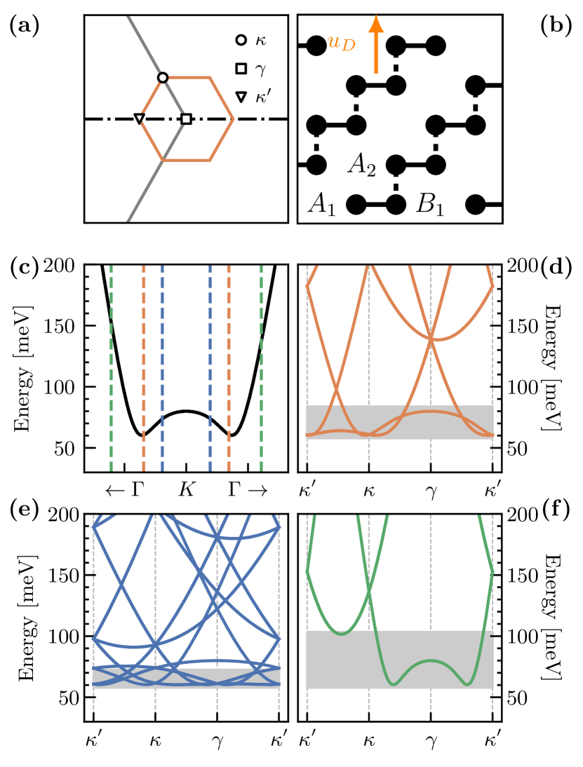
We restrict our attention to a fixed electron density , where we will study the energetic competition between crystalline insulating ground states. In anticipation of spontaneous translation symmetry breaking, we consider a hexagonal “superlattice” generated by , shown in Fig. 1(a). The superlattice size is chosen such that there is one electron per unit cell i.e. filling . While this is not due to an explicitly translation-breaking superlattice potential (e.g. moiré potential), we adopt notation from that context. The band structure is folded (but not yet electronically hybridized) onto a hexagonal mini Brillouin zone (mBZ), Fig. 1(b), with reciprocal lattice vectors and three high-symmetry points and . Fig 1(b) shows and get folded to , while and are folded to . We choose at a high symmetry point before translation breaking. The folded single-particle band structure is three-fold degenerate on the edge of the bottom band at and , which we call mini-valleys. The symmetry enforce degeneracy of the kinetic energy , so the folded band structure is three-fold degenerate.
To make analytic progress, we impose three physical conditions on the ground states. 1) Crystallization: spontaneous symmetry breaking of continuous translations while preserving . This gives a hexagonal “superlattice” with three invariant momenta , and . 2) Weak coupling mean field: the ground state is a Slater determinant state that only hybridizes energetically proximate bands. 3) Three-patch assumption: the single-particle orbitals that make up the ground state wavefunction is essentially homogeneous in large patches around the three invariant momenta. This is in spirit similar to previous “patch models” or “hotspot models” in the superconductivity community [44, 45, 46, 47, 48, 49, 50, 51, 52, 53, 54, 55, 56, 57, 58]. We will argue in App. D that these three conditions can be physically motivated if the band dispersion has a flat bottom and a dispersive edge. Moreover, we verify these three conditions are consistent with SCHF ground states of microscopic model of RMG in Sec. III.
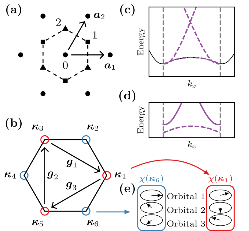
Under these assumptions, the ground states of can be physically modeled by symmetric Slater determinants with one electron at each of the high symmetry points. This procedure is detailed in App. D. Briefly, this follows by taking a single representative -point for each high-symmetry patch, which we conveniently take to be the high-symmetry points. Since the state is weakly coupled, only low-energy bands are allowed to hybridize, giving three states at due to symmetry-enforced band crossings, but generically only one at , as shown in Fig. 1(c). The only possible single-particle wavefunctions are
| (5) | ||||
where we fix the gauge , and the states are indexed by angular momenta defined by
| (6) |
In the above, we fixed the gauge such that .
Given the discrete choices at each momentum point, there are exactly Slater determinant states at filling one electron per -point, which are fully characterized by and . In first quantization,
| (7) |
where is the antisymmetrization operator. Each captures the character of a full 2D state whose Chern number is given by
| (8) |
This follows from the theory of symmetry indicators [33, 59, 60, 61, 62, 63, 64], which posits that the sum of angular momentum at symmetric momenta determines the Chern number mod i.e. . This can be thought of as a generalization of the famous Fu-Kane formula for inversion symmetric topological insulators [33], which was later generalized to discrete rotation symmetries [60]. We choose the origin such that above, implying Eq. (8). We will refer to three possible values of as simply , although in principle the Chern number can be larger.
Due to , these Slater determinant states have degenerate kinetic energy, so their energetic competition is determined solely through interactions:
| (9) |
Below we will evaluate the energies analytically to determine when a state is stabilized.
II.2 Analytical solution of the three-patch model
We will now perform a full analytical evaluation of the three-patch energy in Eq. (9). As it is the energy of a Slater determinant state, we can perform Wick contraction to separate Hartree and Fock contributions:
| (10) |
Here, the Hartree and Fock (exchange) energies between single particle states are defined as
| (11) |
where again is the component of the single-particle wavefunctions at high symmetry point , and the repeated indiced are summed over.
Naively, the interaction energy Eq. (10) comes with three pairs of terms. However, translation by shifts angular momenta , and as we show in App. C. Thus, the energy can only depend on . Since the term does not depend on , it cannot have dependence on angular momenta; the same goes for the term. The only term with dependence on is the term.
By explicit computation in Fourier space, we obtain the energy of the interaction term as a function of :
| (12) | ||||
| (13) |
where we defined form factors , and is the Fourier transform of interaction at momentum . The physical meaning of each term in this sum is clear: they correspond to different scattering processes with momentum transfer .
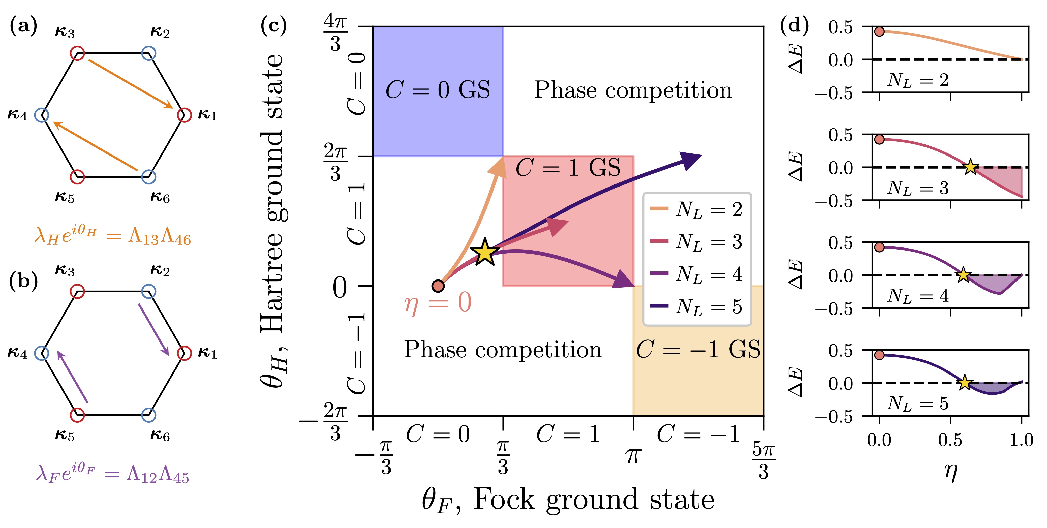
Only the scattering processes depicted in Fig. 2(a, b) and their rotated counterparts have dependence. Collecting those together, and using the action to simplify the expression, we get
| (14) | ||||
| (15) | ||||
| (16) | ||||
Here is a term that does not depend on the Chern number . We parameterized the form factors in terms of two angles
| (17) |
The ground state of is determined by alone. For certain values of and , the ground states of the Hartree and the Fock terms agree, uniquely determining the ground state. In Fig. 2(c), we show a 2D phase diagram of the three-patch model as a function of and . The “frustration free” regions where the Hartree ground state and the Fock ground state agree are shaded with color.
We note these angles are connected to the Pancharatnam overlap
| (18) |
where is defined to be . The angle records the accumulated geometric phase by a path along the mBZ boundaries. In the case where spinors vary slowly along the path, the phase can be approximated by the total Berry curvature within the Brillouin zone. The Fock term starts favoring a state when , which approximately translates to , i.e. half the Berry curvature necessary for the state. The Hartree term, however, favors the state at arbitrarily small , whose competition with the Fock term determines the ultimate ground state.
II.3 Topological Transition from RMG spinors
The phases and can depend on the detail of the spinor structure, which in turn determine whether the is stable. We now consider a concrete example of the spinor to examine the behavior of and . We take the following spinor motivated by the physics of RMG systems:
| (19) |
where is a positive number less than 1, is the normalization factor. The components have action given by .
In Fig. 2(c), we show parametric curves for for various values of . We see that at , the curve never enters the region where both Hartree and Fock terms favor the ground state (labeled as “ GS” in the figure), while for other number of layers, a significant portion of the curve is inside the “ GS” region. We conclude that the AHC state forms at a large range of for , regardless of the values of and .
To see this more quantitatively, we evaluate the Hartree and Fock energies explicitly. They can be organized in powers of (See App. A):
| (20) | ||||
| (21) |
We consider two types of interactions: short-range interaction, i.e. contact interaction (), and long-range interaction, i.e. Coulomb interaction ().
Let us define to be the energy difference between the Coulomb energy of the state and the lowest energy state:
| (22) |
Values signal that is the ground state with the Coulomb interaction. We plot this for in Fig. 2(d). We see that for , becomes the ground state at , marked by a yellow star, while the never becomes the unique ground state for . The corresponding critical point is marked in Fig. 2(c) as well, where the single yellow star covers all the critical points. As the Hartree term always favors the state, the transition point is slightly outside of the “ GS” region. We conclude that the AHC state is favored for large enough for .
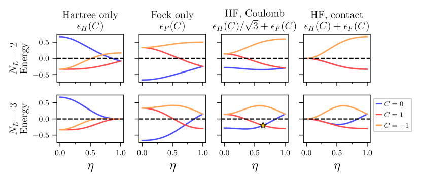
Having understood the case of Coulomb interaction for , we now look at Hartree and Fock contributions separately. Since many of the qualitative features are similar for all , we focus on . We plot the Hartree and Fock energies (), as well as contact and Coulomb energies () in Fig. 3. We note the following features of these plots, which can also be analytically confirmed: 1) Hartree always favors the state, 2) Fock favors the for all values of for , but favors above for , 3) Coulomb interaction energy behaves qualitatively similarly to the Fock interaction energy, and 4) The contact interaction makes and exactly degenerate at , which is a general feature of spinors (which is true in general for , see App. B).
We stress again that the energetics of the phase transition for this choice of spinors is mostly governed by the Fock exchange energy, manifesting in the similarity between the Fock energy curve and the Coulomb energy curve. While the Hartree energy always favors the state, it only shifts the phase transition point slightly.
II.4 Three-patch states in real space
In this section, we inspect the charge density of the three-patch states with RMG spinors, discussed in Sec. II.3. These charge densities are not only characteristic features of the different three-patch states, but also let us peek into their energetics in different regimes.
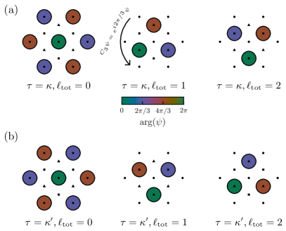
Let us consider the single particle state at with angular momentum . The symmetry of the spinors , fixes the dependence of to the form , where is the angular momentum of spinor component . Using this fact, we can rewrite each component of (Eq. (5) as follows:
| (23) |
The spatial wavefunction is given by
| (24) |
in which is the total angular momentum of the component. At point, it can be written as . The functions for can be obtained by complex conjugation. Some of the key properties of these wavefunctions are reviewed in App. C.
Let us now consider the RMG-inspired spinor, Eq. (19), with :
| (25) |
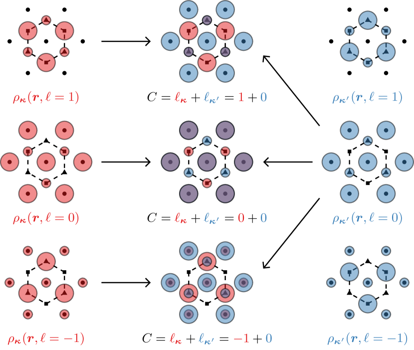
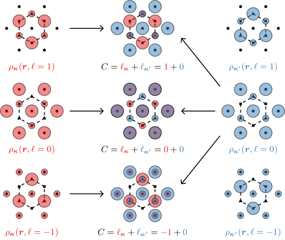
Since the components have different angular momenta , their charge densities appear offset from each other, resulting in the charge density pattern shown in the left column of Fig. 4. We likewise show the charge densities in in the right column.
The total charge densities are simply the sum of these charge densities. We note that for each Chern number, there are three possible charge densities corresponding to different angular momenta. In Sec. III.4, we show that these schematic charge densities agree well with actual SCHF charge densities.
These spatial density patterns can be used to understand some aspects of the energetics of the three-patch states. In App. E, we show that the three-patch charge densities can be used to understand 1) Hartree energy competition between and state, 2) Fock energy competition between and at small , and 3) the stability of the state under honeycomb potential.
We caution the readers that even though the charge densities provide a simple graphical picture to understand some aspects of the energy competition, it also fails to predict many important features. In particular, it does not capture the strength of the Fock interaction at large , thus failing to capture the stability of the AHC state.
III Application of the three-patch model to Rhombohedral Multilayer Graphene
We now introduce a streamlined microscopic model of rhombohedral multilayer graphene (RMG) [65]. We note that our model neglects detailed effects such as lattice relaxation, longer-range hoppings within the rhombohedral graphene, and the layer-dependence of the Coulomb interactions. We also neglect the hBN moiré potential [66, 67, 68, 69], but allow for interaction generated spontaneous translation breaking. We show this simplified model hosts an AHC state within SCHF, and furthermore provides a concrete justification for the three-patch model and its approximations.
III.1 Hamiltonian
Consider layers of graphene with rhombohedral stacking with creation operators where labels sublattice and labels layer. From the side (Fig. 5(d)), RMG forms a staircase with different hopping strengths within and between layers — akin to the SSH chain. The Hamiltonian is
| (26) | ||||
where is the intralayer hopping, is the interlayer hopping, in terms of graphene interatomic vectors , is the graphene lattice constant, and is the electron density on layer . Finally, is a displacement field that polarizes electrons in the conduction bands towards the top layer. We have neglected further-neighbor hoppings for simplicity. The model enjoys rotation symmetry, two-fold rotation , mirror , time-reversal, and standard discrete translations.
We consider an interacting Hamiltonian
| (27) |
where is the charge density operator at wavevector , is the sample area, corresponds to the double-gated Coulomb interactions with gate distance and dielectric (unless otherwise specified). Finally, normal ordering is with respect to the fermionic vacuum at charge neutrality for simplicity. We note this vacuum is strongly renormalized in realistic models in the limit , necessitating “Hartree-Fock subtraction” or other techniques to property renormalize the kinetic term in order to model the realistic system [31]. In the simplified model used here we take only the lowest conduction band to be dynamical.
We often consider a “ghost” superlattice that sets the scale of translation breaking. At superlattice scale we choose mini reciprocal lattice vectors
| (28) |
that generate the mini-Brillouin zone (mBZ) shown in Fig. 5(a). We choose the mBZ to be centered at the graphene point and oriented the same way as the graphene Brillouin zone, with high-symmetry points .
III.2 Spinor structure of RMG
We now investigate the spinor structure of RMG. As has been shown in Sec. II, a fundamental input to the three-patch model are the spinors at the corners of the mBZ, i.e. the points.
We assume the time-reversal symmetry has been broken by spontaneous valley polarization, and focus on near the graphene point. We can simplify Eq. (26) by approximating , where is the graphene Fermi velocity, and . When , the spectrum corresponds to the topological phase of the SSH chain [70, 71]. It hosts two localized boundary modes, polarized on A and B sublattices. The mode has (unnormalized) wavefunction
| (29) |
in the basis . Its normalized counterpart is . The boundary mode is where flips sublattice, and reverses the order of the layers.
If , then the layer edge modes give the that give the highest energy valence band and lowest energy conduction band of RMG. We can thus project the single-particle Hamiltonian into a two-dimensional Hilbert space spanned by and :
| (30) |
where . At small enough , the diagonal part dominates, and we can approximate the energy eigenstate by .
Dropping the sublattices, and performing a layer-dependent gauge transformation, we find that the spinor at the are given by
| (31) |
where
| (32) |
Thus, we recover the spinor structure used in Sec. II.3, allowing us to compare the phenomenology of the section to that of the simplified RMG Hamiltonian.
The critical in the three-patch model, where the state transitions to a state, corresponds to an electronic density of , with a corresponding superlattice length scale of approximately .
III.3 Density range of validity
The band structure of RMG under displacement field, Fig. 5(c), has a relatively flat band bottom, suggesting it could host three-patch states. We now carefully demarcate the density regime where expect the three-patch phenomenology.
Given an electron density, we choose a mini Brillouin Zone (e.g. Eq. (28)) and corresponding superlattice scale so the system is at filling of the superlattice. We then fold the band structure onto the mini-Brillouin zone. Note that since there is no superlattice-scale potential, there is no eigenvalue repulsion.
There is a range of densities in which the minimal model is applicable. The dashed lines in Fig. 5(c) show the mBZ boundaries corresponding to three different densities. Fig. 5(d) shows the band structure at optimal density (orange line), whose lowest band is relatively flat compared to the interaction scale (gray shading), promoting symmetry breaking. Moreover, the large gap to the second band exceeds the interaction scale significantly at , disfavoring mixing. Thus, the ground state is likely to be a weakly coupled symmetry-broken state.
Outside this range of densities, the three-patch assumptions can break down. If the density is too low [Fig. 5(e)], then the other bands will mix strongly at , violating the assumed form of the wavefunction in Eq. (5). This will potentially alter the angular momentum . Alternatively, too large a density [Fig. 5(f)] makes the band too dispersive at the mBZ boundaries, potentially favoring a Fermi liquid over a crystal. Henceforth we focus on the “Goldilocks zone” of densities corresponding to folding the bands near the edge of the flat band bottom.
III.4 Three-patch states as SCHF ground states
In Sec. II, we showed that there is a close energetic competition between and states in the three-patch model using RMG spinors. We now show that the microscopic model Eq. (27) not only realizes this energetic competition, but recapitulates the same real space charge density patterns.
We briefly comment on our SCHF numerics. We explicitly allow translation symmetry breaking by using the folded band structure in the mBZ defined in Eq. (28). We assume valley and spin polarization, resulting from the flavor Stoner ferromagnetism due to the large density of states [72]. We choose the superlattice scale such that the filling is one electron per superlattice unit cell at each density considered. We project to the lowest 7 conduction bands for simplicity, although we note that it may become uncontrolled due to the reduced Hilbert space. See Ref. [29] for further numerical details.
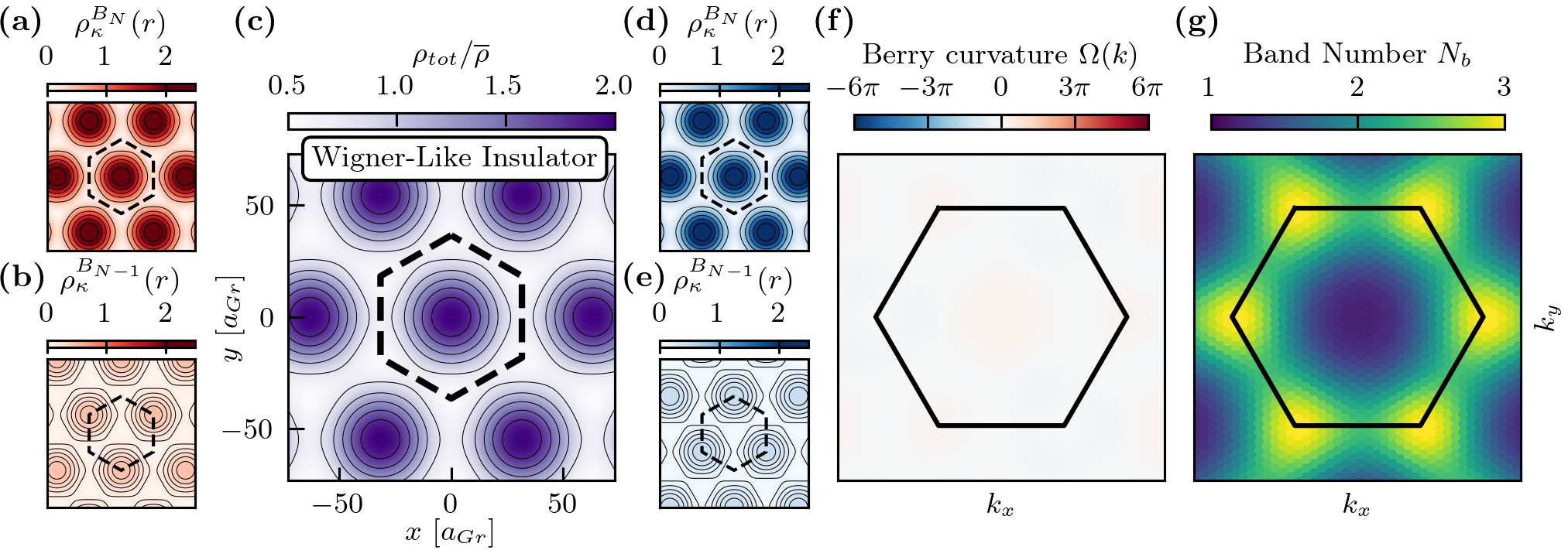
At low densities, corresponding to low , the ground state is a topologically trivial insulator. Its real-space charge density is shown in Fig. 6(c), which has an overall triangular lattice of a Wigner-like insulator — just as in Fig. 4. This charge density is essentially determined by the sum of charge densities from and . In the dominant spinor components, shown in (a) and (d), the charge is centered at the same Wyckoff positions, with the subdominant components “filling in the gaps” to produce the same structure shown in Fig. 10. The Berry curvature, shown in Fig. 6(f) is small everywhere, giving .
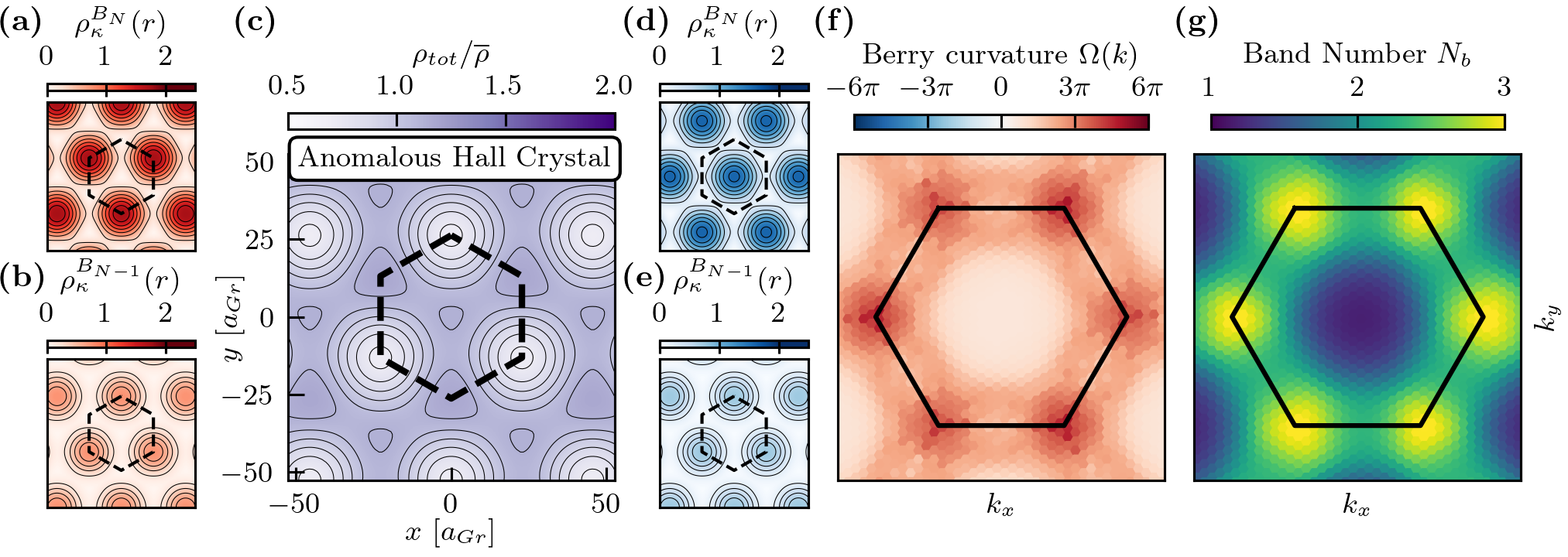
At higher densities, i.e. higher , there is a transition to a state. Fig. 7(c) shows its charge density, which is fairly uniform with peaks on a hexagonal lattice. Now the dominant components are centered on different Wyckoff positions at versus , but the subdominant components are on top of each other. Referring to Fig. 4, we can see this is precisely the same structure as the state there, whose dominant and subdominant components are represented by large and small circles, respectively. Here the Berry curvature, Fig. 7(f), is strongly peaked at and , with a slight breaking.
The success of the three-patch model, which only contains three single-particle wavefunctions, to reproduce the SCHF charge density is consistent with three-patch assumptions. We now explicitly verify that the ground states are weak-coupling states that mix only a few low-lying bands in the folded band structure: this can be revealed by studying the number of single-particle bands of the folded band structure mixed into the occupied band of the SCHF ground state. To quantify this, we note that SCHF eigenstates have the form
| (33) |
where runs over superlattice reciprocal vectors, i.e. different (unhybridized) mini-bands. We define a mini-band distribution function
| (34) |
When the eigenstate is an equal superposition of plane waves (i.e. mini-bands after folding), the von Neumann entropy of the band distribution function equals . Therefore, we define the band number
| (35) |
to quantify the number of bands that mix at each -point.
The band number is shown in Fig. 6,7 (g). It is approximately near , but is close to 3 in at . This confirms that only minibands close to the band bottom appear in the SCHF wavefunction, explicitly confirming the “weak coupling” assumption. In fact, we can see the appearance of large patch-like features near , and . The assumptions of the three-patch model are therefore borne out in microscopic SCHF, so we should expect the phenomenology and predictions of the three-patch model to hold.
III.5 Microscopic verification of the three-patch phase diagram
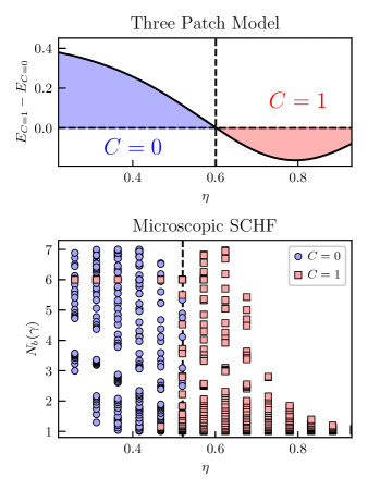
The previous sections demonstrated translation breaking, weak band mixing and clear patches in SCHF ground states of RMG, putting the model into the regime of the three-patch model. We therefore expect the predictions and phenomenology of the three-patch model to appear in the microscopic model. We now show a striking manifestation of this: the competition between and is set by a single parameter .
Fig. 8(a) shows the energy difference between state and the state in the three patch model with Coulomb interaction using spinors from Eq. (29) with . There is a phase transition around . We recall that in RMG, the value of is given by
| (36) |
where is the point for a superlattice such that the electronic density corresponds to .
If is the primary driver of the phase transition between and — as predicted by the three-patch model — there should be a clean phase boundary in terms of alone. To verify this, we first compute the microscopic ground state over a high dimensional parameter space, then dimensionally reduce the results in terms of just two variables. Explicitly, we select and , which quantifies the number of remote bands that mix at the point, and must be close to for the three patch model to be applicable. Concretely, we take , and vary , , and . We identify metallic data points either by a large occupation difference in the mBZ or by a small indirect gap less than . We discard such metallic data points as they are outside the scope of the three-patch model.
The dimensionally-reduced SCHF phase diagram is shown in Fig. 8(b). We see that all of the points above (dashed line) belong to the phase, while most of the points below are in the phase. We note that the and phase boundary in SCHF at goes far beyond the weak coupling point, potentially hinting that the three-patch model works beyond the weak-coupling assumption. We may thus conclude that indeed controls the topological phase transition, and that the three-patch model accurately predicts the critical value. We will comment further on the striking success of the three-patch model in the discussion.
III.6 Three-patch states from analytical mean-field equation
In this brief section, we use a mean field gap equation to analyze the interaction-driven gap. Surprisingly, we find gap opening induces nearly constant wavefunctions in the patches.
Let us focus on a small momentum patch of radius at . At each point in the patch, there are three low-lying states in the Hilbert space of the folded Brillouin zone corresponding to plane waves , , and , defined in Eq. (2). In this three-dimensional Hilbert space, the linearized dispersion of each plane-wave state (before folding) is given by
| (37) |
where is the unit vector parallel to , and is the effective Fermi velocity at the patch. We assume the dispersion is small, since the patch is near a local minimum of dispersion in experimental relevant regimes [see Fig. 5(c)].
We consider a mean-field Hamiltonian by projecting the Hatree and Fock terms into this subspace. By symmetry, it takes the form
| (38) |
where the mean field can be written as
| (39) |
where is the form factor of plane wave states. The first term is the Hartree contribution, whereas the second term is the Fock contribution.
Since we are only interested in the vicinity of , we assume that all the spinors around the points are roughly unchanging:
| (40) |
We also approximate . With these approximations, Eq. (III.6) can be drastically simplified:
| (41) |
Note that now the mean-field potential is independent of , and thus so is the mean-field Hamiltonian Eq. (III.6).
To solve the self-consistent equation Eq. (41), we consider the single-particle Hamiltonian , and solve for the lowest energy single-particle state of . In the absence of the kinetic part , the lowest energy eigenstate takes the form
| (42) |
if we take to be real and negative. We note that the eigenstate at has angular momentum . Now we treat perturbatively, assuming to be small. The lowest energy eigenstate of the full Hamiltonian is given by
| (43) |
Evaluating with , we find
| (44) |
Cancelling from each side, it is easy to see the equation admits a nonzero solution only if the prefactor is positive.
The positivity condition on the prefactor has a quantum geometric interpretation. It can be written as
| (45) |
where is the quantum distance [43]. This inequality is satisfied for physical interactions , revealing a mean field tendency to open a gap. In fact, in the limit of the contact interaction , the left-hand side of the inequality reduces to , revealing that the quantum distance between spinors is a major driving force behind the symmetry breaking tendency. We also note that the positivity of the prefactor is a necessary, but not sufficient, condition for opening a finite gap. Unlike in BCS theory, the -integral does not diverge at , and thus the equation does not hold for an arbitrarily small prefactor. It is amusing to note that the magnitude of the form factors controls the gap, while their phase controls the topology of a resulting insulator.
From Eq. (43), we see that the wavefunctions are all perturbatively close to , controlled by the small ratio , giving rise to a patch-like behavior. The physical interpretation of this is straightforward: the Fock energy favors a large overlap between wavefunctions, similar to how it favors ferromagnetic configuration between spins with large, negative Fock energy. The states around are therefore perturbatively close to each other, controlled by the dispersion that is small around the flat band bottom.
IV Conclusion and outlook
In this work, we constructed a physically-motivated minimal “three-patch model” for the AHC state composed of seven spinor-valued plane waves at the high symmetry points , , and . In the three-patch model, these high symmetry point wavefunctions completely determine both the energetics and the topology of the states, through which we predict the phase diagram of the RMG. The success of the phenomenological three-patch model is striking. Despite its extreme simplicity — with analytic solvability, no kinetic energy, and a vastly reduced Hilbert space — it qualitatively and quantitatively captures the results of microscopic SCHF calculations. This has a fascinating implication: the competition between and is mostly or fully determined by interactions.
Given the example of Wigner crystals, one might expect the topologically trivial electronic crystal to win the energetic competition. But here a crucial extra ingredient is present: the spinor structure. The spinors enter via two geometrical phases, and , that determine the ground state favored by the Hartree and Fock terms respectively. These can compete, but there is a broad “frustration free” regime where Hartree and Fock terms collaborate to favor . In fact, the spinors of RMG fall in this “frustration free” regime in the broad range of the phase diagram.
When comparing careful self-consistent Hartree-Fock results on the simplified RMG Hamiltonian and Coulomb interaction with , we found that the three-patch model successfully described many features of RMG, at least in the weak-coupling regime. In particular, we found that the three-patch model qualitatively reproduced the phase diagram as shown in Fig. 8. The phase boundary between the topological and trivial state was mostly determined by a single parameter of the spinor. Rather surprisingly, the three-patch model also captured the precise charge density pattern obtained from numerics, which in part justifies the effectiveness of our three-patch model.
It is fruitful to consider this unusual mechanism that generated the Berry curvature in the AHC state. Explicitly, the Berry curvature comes from phase-ful superpositions of plane waves produced from gap opening — not just the intrinsic Berry curvature present in the single particle bands before folding. Even if there is only an infinitesimal amount of intrinsic Berry curvature, such as for the spinor at with contact interactions (Fig. 3), the AHC state can still be favored. The AHC thus represents a novel scenario where interaction-driven spontaneous translation breaking is the source of topology. The high density of states regimes without much Berry curvature, which are often realized near the bottom of a band, may thus permit AHC states. We suggest this mechanism opens an unexplored regime where quantized anomalous Hall effects might occur.
In fact, the three-patch model provides a simple algorithm to look for AHC candidate materials: 1) Perform ab initio calculations to look for compound with the band structure with a flat band bottom, 2) Compute the spinor structure near the band bottom, and 3) Compute the quantum geometric phases and . If these phases lie in the “frustration free” region, the compound is a potential AHC candidate.
We note a simple experimental prediction of the three-patch model. Since the critical value of is proportional to , increasing the interlayer hopping by applying pressure would increase the density necessary to stabilize the AHC state. Pressure therefore might drive a quantum phase transition between the AHC state and the Wigner-like insulator state.
An essential future direction is to go beyond mean-field theory. While the three-patch model describes the competition between insulators, it is silent on the competition against an interacting Fermi liquid state. Moreover, there is a fascinating possibility that the AHC state can compete with a fractional anomalous Hall crystal, where a larger unit cell is fractionally occupied, resulting in a translation broken topologically ordered state. Understanding these questions requires analytical or numerical techniques that can treat many strongly-correlated bands, and will be a topic for future work. We hope that the three-patch model will provide valuable insight and phenomenological guidance for such future studies.
Note added—After the completion of this work, Ref. [73] appeared, which proposed a different model system to realize the AHC.
Acknowledgements.
We acknowledge Long Ju, Zhengguan Lu, Tonghang Han, Jixiang Yang, T. Senthil, Trithep Devakul, Yongxin Zeng, Patrick J. Ledwith, Eslam Khalaf, Ruihua Fan, Rahul Sahay, Erez Berg, Dmitry Chichinadze, Chang-Geun Oh, Charlie Marcus, Maksym Serbyn, and Bertrand I. Halperin for insightful discussions. T.W., T.W., and M.Z. are supported by the U.S. Department of Energy, Office of Science, Office of Basic Energy Sciences, Materials Sciences and Engineering Division under Contract No. DE-AC02-05-CH11231 (Theory of Materials program KC2301). T.W. is also supported by the Heising-Simons Foundation, the Simons Foundation, and grant no. PHY-2309135 to the Kavli Institute for Theoretical Physics (KITP). A.V. is supported by the Simons Collaboration on Ultra-Quantum Matter, which is a grant from the Simons Foundation (651440, A.V.) and by the Center for Advancement of Topological Semimetals, an Energy Frontier Research Center funded by the US Department of Energy Office of Science, Office of Basic Energy Sciences, through the Ames Laboratory under contract No. DEAC02-07CH11358. This research is funded in part by the Gordon and Betty Moore Foundation’s EPiQS Initiative, Grant GBMF8683 to T.S. D.E.P. is supported by the Simons Collaboration on Ultra-Quantum Matter, which is a grant from the Simons Foundation.References
- [1] E. Wigner. On the Interaction of Electrons in Metals. Phys. Rev., 46(11):1002–1011, December 1934. Publisher: American Physical Society.
- [2] Yu. E. Lozovik and V. I. Yudson. Crystallization of a two-dimensional electron gas in a magnetic field. Soviet Journal of Experimental and Theoretical Physics Letters, 22:11, July 1975. ADS Bibcode: 1975JETPL..22…11L.
- [3] E. Y. Andrei, G. Deville, D. C. Glattli, F. I. B. Williams, E. Paris, and B. Etienne. Observation of a Magnetically Induced Wigner Solid. Phys. Rev. Lett., 60(26):2765–2768, June 1988. Publisher: American Physical Society.
- [4] M. B. Santos, Y. W. Suen, M. Shayegan, Y. P. Li, L. W. Engel, and D. C. Tsui. Observation of a reentrant insulating phase near the 1/3 fractional quantum Hall liquid in a two-dimensional hole system. Phys. Rev. Lett., 68(8):1188–1191, February 1992. Publisher: American Physical Society.
- [5] J. Falson, I. Sodemann, B. Skinner, D. Tabrea, Y. Kozuka, A. Tsukazaki, M. Kawasaki, K. von Klitzing, and J. H. Smet. Competing correlated states around the zero-field Wigner crystallization transition of electrons in two dimensions. Nat. Mater., 21(3):311–316, March 2022. Publisher: Nature Publishing Group.
- [6] Yen-Chen Tsui, Minhao He, Yuwen Hu, Ethan Lake, Taige Wang, Kenji Watanabe, Takashi Taniguchi, Michael P. Zaletel, and Ali Yazdani. Direct observation of a magnetic field-induced Wigner crystal, December 2023. arXiv:2312.11632 [cond-mat].
- [7] C. C. Grimes and G. Adams. Evidence for a Liquid-to-Crystal Phase Transition in a Classical, Two-Dimensional Sheet of Electrons. Phys. Rev. Lett., 42(12):795–798, March 1979. Publisher: American Physical Society.
- [8] Jongsoo Yoon, C. C. Li, D. Shahar, D. C. Tsui, and M. Shayegan. Wigner Crystallization and Metal-Insulator Transition of Two-Dimensional Holes in GaAs at $B=0$. Phys. Rev. Lett., 82(8):1744–1747, February 1999. Publisher: American Physical Society.
- [9] M. S. Hossain, M. K. Ma, K. A. Villegas Rosales, Y. J. Chung, L. N. Pfeiffer, K. W. West, K. W. Baldwin, and M. Shayegan. Observation of spontaneous ferromagnetism in a two-dimensional electron system. Proceedings of the National Academy of Sciences, 117(51):32244–32250, December 2020. Publisher: Proceedings of the National Academy of Sciences.
- [10] Tomasz Smoleński, Pavel E. Dolgirev, Clemens Kuhlenkamp, Alexander Popert, Yuya Shimazaki, Patrick Back, Xiaobo Lu, Martin Kroner, Kenji Watanabe, Takashi Taniguchi, Ilya Esterlis, Eugene Demler, and Ataç Imamoğlu. Signatures of Wigner crystal of electrons in a monolayer semiconductor. Nature, 595(7865):53–57, July 2021. Publisher: Nature Publishing Group.
- [11] You Zhou, Jiho Sung, Elise Brutschea, Ilya Esterlis, Yao Wang, Giovanni Scuri, Ryan J. Gelly, Hoseok Heo, Takashi Taniguchi, Kenji Watanabe, Gergely Zaránd, Mikhail D. Lukin, Philip Kim, Eugene Demler, and Hongkun Park. Bilayer Wigner crystals in a transition metal dichalcogenide heterostructure. Nature, 595(7865):48–52, July 2021. Publisher: Nature Publishing Group.
- [12] Fangyuan Yang, Alexander A. Zibrov, Ruiheng Bai, Takashi Taniguchi, Kenji Watanabe, Michael P. Zaletel, and Andrea F. Young. Experimental Determination of the Energy per Particle in Partially Filled Landau Levels. Phys. Rev. Lett., 126(15):156802, April 2021. Publisher: American Physical Society.
- [13] Jiho Sung, Jue Wang, Ilya Esterlis, Pavel A. Volkov, Giovanni Scuri, You Zhou, Elise Brutschea, Takashi Taniguchi, Kenji Watanabe, Yubo Yang, Miguel A. Morales, Shiwei Zhang, Andrew J. Millis, Mikhail D. Lukin, Philip Kim, Eugene Demler, and Hongkun Park. Observation of an electronic microemulsion phase emerging from a quantum crystal-to-liquid transition, December 2023. arXiv:2311.18069 [cond-mat].
- [14] Ziyu Xiang, Hongyuan Li, Jianghan Xiao, Mit H. Naik, Zhehao Ge, Zehao He, Sudi Chen, Jiahui Nie, Shiyu Li, Yifan Jiang, Renee Sailus, Rounak Banerjee, Takashi Taniguchi, Kenji Watanabe, Sefaattin Tongay, Steven G. Louie, Michael F. Crommie, and Feng Wang. Quantum Melting of a Disordered Wigner Solid, February 2024. arXiv:2402.05456 [cond-mat].
- [15] Steven Kivelson, C. Kallin, Daniel P. Arovas, and J. R. Schrieffer. Cooperative ring exchange theory of the fractional quantized Hall effect. Phys. Rev. Lett., 56(8):873–876, February 1986. Publisher: American Physical Society.
- [16] B. I. Halperin, Z. Tešanović, and F. Axel. Compatibility of Crystalline Order and the Quantized Hall Effect. Phys. Rev. Lett., 57(7):922–922, August 1986. Publisher: American Physical Society.
- [17] Steven Kivelson, C. Kallin, Daniel P. Arovas, and J. Robert Schrieffer. Cooperative ring exchange and the fractional quantum Hall effect. Phys. Rev. B, 36(3):1620–1646, July 1987. Publisher: American Physical Society.
- [18] Zlatko Tešanović, Françoise Axel, and B. I. Halperin. “Hall crystal” versus Wigner crystal. Phys. Rev. B, 39(12):8525–8551, April 1989. Publisher: American Physical Society.
- [19] Zhengguang Lu, Tonghang Han, Yuxuan Yao, Aidan P. Reddy, Jixiang Yang, Junseok Seo, Kenji Watanabe, Takashi Taniguchi, Liang Fu, and Long Ju. Fractional quantum anomalous Hall effect in multilayer graphene. Nature, 626(8000):759–764, February 2024. Number: 8000 Publisher: Nature Publishing Group.
- [20] N. Regnault and B. Andrei Bernevig. Fractional Chern Insulator. Phys. Rev. X, 1(2):021014, December 2011. Publisher: American Physical Society.
- [21] Evelyn Tang, Jia-Wei Mei, and Xiao-Gang Wen. High-Temperature Fractional Quantum Hall States. Phys. Rev. Lett., 106(23):236802, June 2011. Publisher: American Physical Society.
- [22] Kai Sun, Zhengcheng Gu, Hosho Katsura, and S. Das Sarma. Nearly Flatbands with Nontrivial Topology. Phys. Rev. Lett., 106(23):236803, June 2011. Publisher: American Physical Society.
- [23] Titus Neupert, Luiz Santos, Claudio Chamon, and Christopher Mudry. Fractional Quantum Hall States at Zero Magnetic Field. Phys. Rev. Lett., 106(23):236804, June 2011. Publisher: American Physical Society.
- [24] Emil J. Bergholtz and Zhao Liu. Topological flat band models and fractional chern insulators. Int. J. Mod. Phys. B, 27(24):1330017, September 2013. Publisher: World Scientific Publishing Co.
- [25] Zhao Liu and Emil J. Bergholtz. Recent developments in fractional Chern insulators. In Tapash Chakraborty, editor, Encyclopedia of Condensed Matter Physics (Second Edition), pages 515–538. Academic Press, Oxford, January 2024.
- [26] Guorui Chen, Aaron L. Sharpe, Eli J. Fox, Ya-Hui Zhang, Shaoxin Wang, Lili Jiang, Bosai Lyu, Hongyuan Li, Kenji Watanabe, Takashi Taniguchi, Zhiwen Shi, T. Senthil, David Goldhaber-Gordon, Yuanbo Zhang, and Feng Wang. Tunable correlated Chern insulator and ferromagnetism in a moiré superlattice. Nature, 579(7797):56–61, March 2020. Number: 7797 Publisher: Nature Publishing Group.
- [27] Zhihuan Dong, Adarsh S. Patri, and T. Senthil. Theory of fractional quantum anomalous Hall phases in pentalayer rhombohedral graphene moir\’e structures, November 2023. arXiv:2311.03445 [cond-mat].
- [28] Boran Zhou, Hui Yang, and Ya-Hui Zhang. Fractional quantum anomalous Hall effects in rhombohedral multilayer graphene in the moir\’eless limit and in Coulomb imprinted superlattice, November 2023. arXiv:2311.04217 [cond-mat].
- [29] Junkai Dong, Taige Wang, Tianle Wang, Tomohiro Soejima, Michael P. Zaletel, Ashvin Vishwanath, and Daniel E. Parker. Anomalous Hall Crystals in Rhombohedral Multilayer Graphene I: Interaction-Driven Chern Bands and Fractional Quantum Hall States at Zero Magnetic Field, November 2023. arXiv:2311.05568 [cond-mat].
- [30] Zhongqing Guo, Xin Lu, Bo Xie, and Jianpeng Liu. Theory of fractional Chern insulator states in pentalayer graphene moir\’e superlattice, December 2023. arXiv:2311.14368 [cond-mat].
- [31] Yves H. Kwan, Jiabin Yu, Jonah Herzog-Arbeitman, Dmitri K. Efetov, Nicolas Regnault, and B. Andrei Bernevig. Moir\’e Fractional Chern Insulators III: Hartree-Fock Phase Diagram, Magic Angle Regime for Chern Insulator States, the Role of the Moir\’e Potential and Goldstone Gaps in Rhombohedral Graphene Superlattices, December 2023. arXiv:2312.11617 [cond-mat].
- [32] B. Andrei Bernevig, Taylor L. Hughes, and Shou-Cheng Zhang. Quantum Spin Hall Effect and Topological Phase Transition in HgTe Quantum Wells. Science, 314(5806):1757–1761, December 2006. Publisher: American Association for the Advancement of Science.
- [33] Liang Fu and C. L. Kane. Topological insulators with inversion symmetry. Phys. Rev. B, 76(4):045302, July 2007. Publisher: American Physical Society.
- [34] Chaoxing Liu, Taylor L. Hughes, Xiao-Liang Qi, Kang Wang, and Shou-Cheng Zhang. Quantum Spin Hall Effect in Inverted Type-II Semiconductors. Phys. Rev. Lett., 100(23):236601, June 2008. Publisher: American Physical Society.
- [35] Haijun Zhang, Chao-Xing Liu, Xiao-Liang Qi, Xi Dai, Zhong Fang, and Shou-Cheng Zhang. Topological insulators in Bi2Se3, Bi2Te3 and Sb2Te3 with a single Dirac cone on the surface. Nature Phys, 5(6):438–442, June 2009. Publisher: Nature Publishing Group.
- [36] Jinwu Ye, Yong Baek Kim, A. J. Millis, B. I. Shraiman, P. Majumdar, and Z. Tešanović. Berry Phase Theory of the Anomalous Hall Effect: Application to Colossal Magnetoresistance Manganites. Phys. Rev. Lett., 83(18):3737–3740, November 1999. Publisher: American Physical Society.
- [37] Kenya Ohgushi, Shuichi Murakami, and Naoto Nagaosa. Spin anisotropy and quantum Hall effect in the kagom\’e lattice: Chiral spin state based on a ferromagnet. Phys. Rev. B, 62(10):R6065–R6068, September 2000. Publisher: American Physical Society.
- [38] Keita Hamamoto, Motohiko Ezawa, and Naoto Nagaosa. Quantized topological Hall effect in skyrmion crystal. Phys. Rev. B, 92(11):115417, September 2015. Publisher: American Physical Society.
- [39] Kevin A. van Hoogdalem, Yaroslav Tserkovnyak, and Daniel Loss. Magnetic texture-induced thermal Hall effects. Phys. Rev. B, 87(2):024402, January 2013. Publisher: American Physical Society.
- [40] Fengcheng Wu, Timothy Lovorn, Emanuel Tutuc, Ivar Martin, and A. H. MacDonald. Topological Insulators in Twisted Transition Metal Dichalcogenide Homobilayers. Phys. Rev. Lett., 122(8):086402, February 2019. Publisher: American Physical Society.
- [41] Nisarga Paul and Liang Fu. Topological magnetic textures in magnetic topological insulators. Phys. Rev. Res., 3(3):033173, August 2021. Publisher: American Physical Society.
- [42] Stefan Divic, Henry Ling, T. Pereg-Barnea, and Arun Paramekanti. Magnetic skyrmion crystal at a topological insulator surface. Phys. Rev. B, 105(3):035156, January 2022. Publisher: American Physical Society.
- [43] Arno Böhm, Ali Mostafazadeh, Hiroyasu Koizumi, Qian Niu, and Josef Zwanziger. The Geometric phase in quantum systems: foundations, mathematical concepts, and applications in molecular and condensed matter physics. Springer, 2003.
- [44] John A. Hertz. Quantum critical phenomena. Phys. Rev. B, 14:1165–1184, Aug 1976.
- [45] A. J. Millis. Effect of a nonzero temperature on quantum critical points in itinerant fermion systems. Phys. Rev. B, 48:7183–7196, Sep 1993.
- [46] Rahul Nandkishore, Ronny Thomale, and Andrey V. Chubukov. Superconductivity from weak repulsion in hexagonal lattice systems. Phys. Rev. B, 89:144501, Apr 2014.
- [47] Ar. Abanov and Andrey V. Chubukov. Spin-fermion model near the quantum critical point: One-loop renormalization group results. Phys. Rev. Lett., 84:5608–5611, Jun 2000.
- [48] Ar. Abanov and A. Chubukov. Anomalous scaling at the quantum critical point in itinerant antiferromagnets. Phys. Rev. Lett., 93:255702, Dec 2004.
- [49] Max A. Metlitski and Subir Sachdev. Quantum phase transitions of metals in two spatial dimensions. ii. spin density wave order. Phys. Rev. B, 82:075128, Aug 2010.
- [50] Seth Whitsitt and Subir Sachdev. Renormalization group analysis of a fermionic hot-spot model. Phys. Rev. B, 90:104505, Sep 2014.
- [51] H. J. Schulz. Superconductivity and antiferromagnetism in the two-dimensional hubbard model: Scaling theory. Europhysics Letters, 4(5):609, sep 1987.
- [52] I. E. Dzialoshinskii. The superconducting transitions due to Van Hove singularities in the electron spectrum. Zhurnal Eksperimentalnoi i Teoreticheskoi Fiziki, 93:1487–1498, October 1987.
- [53] Lederer, P., Montambaux, G., and Poilblanc, D. Antiferromagnetism and superconductivity in a quasi two-dimensional electron gas. scaling theory of a generic hubbard model. J. Phys. France, 48(10):1613–1618, 1987.
- [54] Nobuo Furukawa, T. M. Rice, and Manfred Salmhofer. Truncation of a two-dimensional fermi surface due to quasiparticle gap formation at the saddle points. Phys. Rev. Lett., 81:3195–3198, Oct 1998.
- [55] Karyn Le Hur and T. Maurice Rice. Superconductivity close to the mott state: From condensed-matter systems to superfluidity in optical lattices. Annals of Physics, 324(7):1452–1515, 2009. July 2009 Special Issue.
- [56] Rahul Nandkishore, L. S. Levitov, and A. V. Chubukov. Chiral superconductivity from repulsive interactions in doped graphene. Nature Physics, 8(2):158–163, Feb 2012.
- [57] Hiroki Isobe, Noah F. Q. Yuan, and Liang Fu. Unconventional superconductivity and density waves in twisted bilayer graphene. Phys. Rev. X, 8:041041, Dec 2018.
- [58] Da-Chuan Lu, Taige Wang, Shubhayu Chatterjee, and Yi-Zhuang You. Correlated metals and unconventional superconductivity in rhombohedral trilayer graphene: A renormalization group analysis. Phys. Rev. B, 106:155115, Oct 2022.
- [59] Ari M. Turner, Yi Zhang, Roger S. K. Mong, and Ashvin Vishwanath. Quantized response and topology of magnetic insulators with inversion symmetry. Phys. Rev. B, 85(16):165120, April 2012. Publisher: American Physical Society.
- [60] Chen Fang, Matthew J. Gilbert, and B. Andrei Bernevig. Bulk topological invariants in noninteracting point group symmetric insulators. Phys. Rev. B, 86(11):115112, September 2012. Publisher: American Physical Society.
- [61] Hoi Chun Po, Ashvin Vishwanath, and Haruki Watanabe. Symmetry-based indicators of band topology in the 230 space groups. Nat Commun, 8(1):50, June 2017. Number: 1 Publisher: Nature Publishing Group.
- [62] Barry Bradlyn, L. Elcoro, Jennifer Cano, M. G. Vergniory, Zhijun Wang, C. Felser, M. I. Aroyo, and B. Andrei Bernevig. Topological quantum chemistry. Nature, 547(7663):298–305, July 2017. Number: 7663 Publisher: Nature Publishing Group.
- [63] Hoi Chun Po. Symmetry indicators of band topology. J. Phys.: Condens. Matter, 32(26):263001, April 2020. Publisher: IOP Publishing.
- [64] Jennifer Cano and Barry Bradlyn. Band Representations and Topological Quantum Chemistry. Annual Review of Condensed Matter Physics, 12(1):225–246, 2021. _eprint: https://doi.org/10.1146/annurev-conmatphys-041720-124134.
- [65] Fan Zhang, Bhagawan Sahu, Hongki Min, and A. H. MacDonald. Band structure of A B C -stacked graphene trilayers. Phys. Rev. B, 82(3):035409, July 2010.
- [66] Jeil Jung, Arnaud Raoux, Zhenhua Qiao, and A. H. MacDonald. Ab initio theory of moiré superlattice bands in layered two-dimensional materials. Phys. Rev. B, 89(20):205414, May 2014.
- [67] Pilkyung Moon and Mikito Koshino. Electronic properties of graphene/hexagonal-boron-nitride moiré superlattice. Phys. Rev. B, 90(15):155406, October 2014.
- [68] Ya-Hui Zhang, Dan Mao, Yuan Cao, Pablo Jarillo-Herrero, and T. Senthil. Nearly flat Chern bands in moir\’e superlattices. Phys. Rev. B, 99(7):075127, February 2019. Publisher: American Physical Society.
- [69] Youngju Park, Yeonju Kim, Bheema Lingam Chittari, and Jeil Jung. Topological flat bands in rhombohedral tetralayer and multilayer graphene on hexagonal boron nitride moire superlattices, April 2023. arXiv:2304.12874 [cond-mat].
- [70] Ruijuan Xiao, F. Tasnádi, K. Koepernik, J. W. F. Venderbos, M. Richter, and M. Taut. Density functional investigation of rhombohedral stacks of graphene: Topological surface states, nonlinear dielectric response, and bulk limit. Phys. Rev. B, 84(16):165404, October 2011. Publisher: American Physical Society.
- [71] W. P. Su, J. R. Schrieffer, and A. J. Heeger. Solitons in Polyacetylene. Phys. Rev. Lett., 42(25):1698–1701, June 1979. Publisher: American Physical Society.
- [72] Haoxin Zhou, Tian Xie, Areg Ghazaryan, Tobias Holder, James R. Ehrets, Eric M. Spanton, Takashi Taniguchi, Kenji Watanabe, Erez Berg, Maksym Serbyn, and Andrea F. Young. Half- and quarter-metals in rhombohedral trilayer graphene. Nature, 598(7881):429–433, October 2021. Number: 7881 Publisher: Nature Publishing Group.
- [73] Yongxin Zeng, Daniele Guerci, Valentin Crépel, Andrew J. Millis, and Jennifer Cano. Sublattice structure and topology in spontaneously crystallized electronic states, February 2024. arXiv:2402.17867 [cond-mat].
Appendix A Derivation of Hartree and Fock energies for RMG spinors
We evaluate the Hartree and Fock energies Eqs. (20,21) explicitly. Recall that the spinor is given by
| (46) |
where .
The form factor is defined by . Then,
| (47) | ||||
| (48) |
Therefore, we get
| (49) | ||||
| (50) | ||||
| (51) | ||||
| (52) |
Similarly, we get for Fock
| (53) | ||||
| (54) | ||||
| (55) | ||||
| (56) |
Appendix B Proof of degeneracy under contact interaction
We will now prove the curious fact that if and spinors only have two components (with angular momentum and , respectively), then the Chern number and states will remain degenerate under contact interaction.
We now define
| (57) |
The action is given again by . We fix the gauge such that .
In contact interactions, we can take . Thus
| (60) |
which means that . We note that contact interaction annihilates all intra-orbital interactions, and one can generally prove that the and states are still degenerate under any inter-orbital interaction.
Appendix C Real space properties of orbitals at and
In this appendix, we will explain two elementary characteristics of symmetric orbitals at and points. Recall that Wyckoff positions are points in the unit cell that are invariant under a spatial symmetry action. With the current choice of the lattice, these points are integer multiples of
| (61) |
Below we will establish the following two facts:
-
1.
The orbital-resolved charge densities of symmetric states at and points have peaks and zeros at the Wyckoff points, determined by both the orbital angular momentum and the state angular momentum ;
-
2.
The action of the translation translates , and .
To understand the first statement, take the point without loss of generality. Now, consider the state : its orbital-resolved charge density is given by
| (62) |
We now make use of the definition Eq. (5). Consider the momentum point : Let’s say . Then, due to the gauge choice , we have , and similarly .
We may now compute the angular-momentum resolved charge density:
| (63) | ||||
Since for and for (modulo ), we may immediately deduce
| (64) |
where the if and otherwise.
This motivates a definition of
| (65) |
Indeed, a similar calculation for the shows that
| (66) |
where labels the and points.
This establishes the first fact: the peak of the charge density is at a Wyckoff position determined by a signed total angular momentum, . Particularly, one can see in Fig. 9 that although the charge density peaks of at point and at point share the same Wyckoff positions, the wavefunctions have different phase structures and thus different angular momenta.
As for the second fact, we show it explicitly:
| (67) | ||||
The point calculation is exactly similar. Both of these statements can be checked graphically in Fig. 9.
Appendix D Justification of the three-patch model
In this appendix, we will motivate the building blocks of the three-patch model from simple physical conditions of the single-particle band structure. We will also discuss how we arrive at the restricted Hilbert space in Eq. (5) and below.
Spontaneous translation symmetry breaking can occur in the case that the interaction strength is much larger than the bandwidth of the lowest band within the mBZ:
| (68) |
In the limit where the lowest band is completely flat, the Fermi surface can be arbitrarily deformed without being penalized by the kinetic energy. In this way, we can create low-energy Fermi surfaces with perfect nesting conditions, which are in general unstable to the creation of insulating states by the exchange interaction. This thus corresponds to condition (i) stated at the beginning of Sec. II. Once we take the dispersion into account, a gap equation must be solved to investigate the existence of such instabilities, which is performed under various approximations in Sec. III.6.
The “weak coupling mean field” assumption has two subparts. It firstly states that the state is weakly coupled. This can also be implemented by an energetic constraint: we need a large gap between the point and its higher harmonics, which means that there will be a large direct gap around the point in the folded band structure. In the case where
| (69) |
interactions cannot hybridize the point wavefunction with other plane waves, and thus the state will be weakly coupled. It also states that the state can be described as a Slater determinant state. While this mean-field approximation is uncontrolled, as long as we consider a variational space of Hartree-Fock states, this assumption is always satisfied.
The three-patch assumption is harder to justify a priori from the knowledge of the single-particle Hamiltonian alone. Physically, the Fock interaction is strong between nearby momentum given the small momentum exchange, and thus the single particle wavefunctions can be plausibly inferred to be similar. However, realistically, the best we can do is an a posteriori justification by inspecting the nature of the SCHF ground state, which we have performed carefully for the ground states of the RMG Hamiltonian.
In the remainder of this section, we will explain in detail how to physically obtain the reduced Hilbert space Eq. (5) from the assumptions above.
We only consider Slater determinant states. After we fold the Brillouin zone, the states are then labeled by crystalline momentum :
| (70) |
where is the occupation number at mBZ momentum , and is the creation operator with mBZ momentum . Since we assumed the state to be an insulator, we fill the low-energy band of the mean-field Hamiltonian in the mBZ such that for all crystalline momentum .
The weak-coupling assumption then allows us to reduce to a low-energy Hilbert space with the lowest energy plane waves. Explicitly, we can restrict to a Slater determinant states generated by low energy plane waves:
| (71) |
Here the sum over is only non-zero when is small relative to the interaction strength.
Finally, the three-patch enables a further reduction to an analytically tractable model. Since the wavefunction is assumed to be homogeneous within each patch, we pick one representative momentum to describe the whole patch. The most natural choice is the set of high symmetry points . Schematically, this reduction in Hilbert space can be written as:
| (72) |
The high symmetry points have one, three, and three low-energy states respectively. We will assume that electronic states from the higher shells have a gap to these low-energy states that is much larger compared to the interaction energy. Following (71), and symmetry, the associated creation operators are , and with angular momentum . Their single-particle wavefunctions are thus given by Eq. (5), which we reproduce here
| (73) | ||||
By the assumption that we have an insulating state with , we have one electron per representative state in the patch. Together with the Slater determinant assumption, we arrive at variational states
| (74) |
This establishes the three-patch model.
Appendix E Energetic competition of the three-patch states
We now use the charge density pattern above to infer some features of the Hartree and Fock energies. The Hartree energy between and corresponds to the interaction energy of classical charge configurations. It now becomes a simple visual exercise: we can visually figure out which charge densities are on top of each other by looking at Fig. 10. It is easy to see that the state has the least density overlap between . This is confirmed in the Hartree energy plot in Fig. 10.
At small , the Fock term can be similarly graphically evaluated. This is because Fock exchange energy is controlled by the alignment of pseudospins, and at small most weight is on the top layer. We conclude the state has the lowest Fock energy due to the large overlap between the top layer charge densities, as confirmed in the Fock energy plot in Fig. 10. We note, however, that this visual exercise misses other contributions such as intercomponent interactions, and is qualitatively incorrect at large , as evidenced by the fact that state can have lower Fock energy.
We note an interesting implication of the density patterns. Consider a potential such that , where . This potential has a honeycomb shape, where the electrons are favored to form a triangular lattice at the superlattice points. If we apply this potential to the first component of the spinor, the state, which has a triangular charge density in the first component, gains more energy than states. On the other hand, if the potential is applied to the second component, the state is favored over the other states, since the charge density of the second component forms a triangular lattice. This consideration implies that the phase boundary can be shifted by such external potentials.