Volume-entangled exact eigenstates in the PXP and related models in any dimension

Abstract

In this work, we describe an approach for unveiling many-body Einstein-Podolsky-Rosen-like volume-entangled exact scars hosted by diverse PXP-type models for Rydberg-blockaded atom systems and discuss experimentally relevant aspects of these previously unknown states.

Introduction

The observation of unusually slow thermalization dynamics and unexpected many-body revivals during a quench from a Néel-type state in the pioneering Rydberg atom experiment [1] ignited significant interest in the so-called PXP model [2], which is an idealized description of Rydberg atomic systems in the nearest-neighbor blockade regime. The attribution of this atypical dynamics to the presence of the special “scar” eigenstates weakly violating the eigenstate thermalization hypothesis (ETH) in the spectrum of the one-dimensional PXP Hamiltonian [3, 4] opened the field of quantum many-body scars [5, 6, 7]. Although various perspectives on the mechanisms leading to the emergence of these states have been put forth [3, 4, 8, 9, 10, 11, 12, 13, 14, 15, 16, 17], no comprehensive theory explaining ETH-violating phenomena in systems evolving under PXP-type Hamiltonians is currently available (for reviews of this and broader scar topics see [18, 19, 20, 21]). Despite its apparent simplicity, the PXP Hamiltonian, being non-integrable and chaotic based on the level statistics, typically eludes analytical treatment, which is evident from the scarcity of exact results, even though much effort has been dedicated to its study in the recent years. For example, only two exact zero energy eigenstates related by translation are currently known for the PXP chain with periodic boundary conditions (PBC) [9]; exponentially many states with valence bond solid orders have been found in two-dimensional PXP models [22, 23]. All currently known exact eigenstates exhibit area law scaling of entanglement.

In this work, we report first exact volume-entangled scar states hosted by various PXP-type models including the paradigmatic and most extensively studied ones, such as the PBC chain and square lattice. We start by introducing a new zero-energy eigenstate of the PBC chain and proceed by generalizing its structure to a wide variety of geometries. We point out the experimental relevance of this new type of states by providing a concrete and feasible protocol for their preparation on near-term Rydberg quantum devices[24, 25, 26, 27, 28, 29, 30, 31, 32, 33], which relies only on strictly local measurements and evolution under the natural PXP-type Hamiltonian. We also provide examples of the utility of these new eigenstates for studying non-trivial quantum dynamics such as out-of-time-order correlator (OTOC) functions, and discuss their possible applicability to fidelity benchmarking and quantum advantage problems.

Eigenstate of the PXP chain

Consider a state on a spin-1/2 chain of size $N=2L$ with PBC defined as

$$\ket{\Lambda}=\frac{1}{\sqrt{\chi}}\sum_{f\in\mathcal{F}^{(p)}_{L}}(-1)^{|f|}\ket{f}_{1,\ldots,L}\otimes\ket{f}_{L+1,\ldots,2L},$$ (1)

where $\mathcal{F}^{(p)}_{L}$ is the set of bitstrings defining the nearest neighbour Rydberg blockaded subspace for chains of $L$ spins with PBC, $|f|$ stands for the parity of the bitstring $f$, and, in terms of the Fibonacci numbers $F_{n}$, $\chi=\left|\mathcal{F}^{(p)}_{L}\right|=F_{L-1}+F_{L+1}$ (see Fig. 1 illustrating $\ket{\Lambda}$).

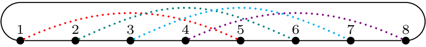
Figure 1: State $\ket{\Lambda}$ on an $N=2L=8$ PBC chain. Dotted lines indicate the pairing pattern of perfectly correlated spins.

By inspection, each $\ket{f}\otimes\ket{f}$ in Eq. (1) satisfies the Rydberg blockade on the full PBC chain; $\ket{\Lambda}$ is invariant under the global “particle-hole” symmetry operator $C_{\text{ph}}=\prod_{i=1}^{N}Z_{i}$ (where $Z_{i}\equiv\outerproduct{0}{0}_{i}-\outerproduct{1}{1}_{i}$), arbitrary bond or site inversions, and translation by one site. It is also invariant under the pseudo-local $\text{SWAP}_{i,i+L}$ and $Z_{i}Z_{i+L}$ unitaries. We claim that $\ket{\Lambda}$ is an exact zero energy eigenstate of the Hamiltonian

$$H_{\text{PXP}}(N)=\sum_{i=1}^{N}P_{i-1}X_{i}P_{i+1},\quad(i\equiv i+N),$$ (2)

where $P_{i}\equiv\outerproduct{0}{0}_{i}$ and $X_{i}\equiv\outerproduct{1}{0}_{i}+\outerproduct{0}{1}_{i}$.

For any $f\in\mathcal{F}^{(p)}_{L}$, the neighborhoods of spins $1$ and $L$ ($L+1$ and $2L$) are identical in $\ket{f}_{1,\ldots,L}$ ($\ket{f}_{L+1,\ldots,2L}$) and $\ket{f}_{1,\ldots,L}\otimes\ket{f}_{L+1,\ldots,2L}$ if PBC are assumed in the half-system $[1,\dots,L]$ ($[L+1,\dots,2L]$) and the actual system $[1,\dots,2L]$. This means that the action of $H_{\text{PXP}}(N)$ on $\ket{\Lambda}$ is equivalent to the action of the “disconnected-halves” (DH) Hamiltonian $H_{\text{DH}}(L)$ — i.e., $H_{\text{DH}}(L)\ket{\Lambda}=H_{\text{PXP}}(N)\ket{\Lambda}$ — written as a sum of two decoupled PXP Hamiltonians with half-system PBC:

$$H_{\text{DH}}(L)=H_{\text{PXP}}^{\text{left}}(L)_{1,\ldots,L}+H_{\text{PXP}}^{\text{right}}(L)_{L+1,\ldots,2L}.$$ (3)

It is then easy to show that $H_{\text{PXP}}^{\text{left}}(L)\ket{\Lambda}=-H_{\text{PXP}}^{\text{right}}(L)\ket{\Lambda}$, and thus $H_{\text{PXP}}(N)\ket{\Lambda}=H_{\text{DH}}(L)\ket{\Lambda}=0$ (see Sec. I. of the Supplemental Material [34]).

The same argument holds for Hamiltonians with terms of the form $A_{[i-m,\dots,i-1]}X_{i}B_{[i+1,\dots,i+n]}$, where $A$ and $B$ are arbitrary diagonal in the computational basis operators with support on, respectively, $m$ and $n$ sites to the left and to the right of $i$, in particular for all deformations of the Rydberg blockade Hamiltonian in Refs. [8, 10, 35]. Also, terms at different locations can come with different couplings as long as they are identical for sites $i$ and $i+L$; the only necessary condition is that the action of $H_{\text{PXP}}^{\text{left}}(L)$ is identical to that of $H_{\text{PXP}}^{\text{right}}(L)$, and that this action only connects basis states with opposite parities. In particular, if $L$ is even, the nullspaces of Hamiltonians $H_{o}$ and $H_{e}$ defined by restricting the sum in Eq. (2) to, respectively, odd and even sites both contain $\ket{\Lambda}$, which means this state is invariant under Floquet unitaries $U^{o/e}_{\tau}=e^{-iH_{o/e}\tau}$ used to define the Floquet PXP model in Refs. [36, 37, 17]. Similar arguments hold also for models with extended Rydberg blockades, in which case $\mathcal{F}_{L}^{(p)}$ in Eq. (1) should be substituted for a set of bitstrings corresponding to an appropriate constrained Hilbert space. Generalizations discussed in this paragraph also apply to states introduced in later sections.

Tracing over half of the chain in Eq. (1) gives a reduced density matrix of the maximally mixed Gibbs ensemble of a Rydberg-blockaded PBC chain of size $L$ (thus the von Neumann entanglement entropy $\mathcal{S}_{1/2}=\log\chi$; i.e., $\mathcal{S}_{1/2}\propto L$); any observable with support on a geometrically connected half-system is distributed as if it is sampled from such infinite-temperature ensemble. In contrast, non-local observables on sites separated by distance $L$ have highly non-thermal expectation values due to perfect correlation between the spins. For a detailed discussion of the entanglement structure of $\ket{\Lambda}$ see Sec. II. of the Supplemental Material [34].

Relation to other volume-entangled states

Various volume-entangled states constructed on a doubled Hilbert space appeared in the literature; most notably, the thermofield-double state (TFD) [38, 39], its infinite-temperature variant, the many-body Einstein-Podolsky-Rosen (EPR) state [39], and the rainbow scars [40]. Defined on the same Hilbert space, $\ket{\Lambda}$ and the EPR state would differ only by the phases depending on the parity of each half-system basis state in the former.

To see the connection with the rainbow scars, let us formulate $\ket{\Lambda}$ within the framework presented in [40]. Let $H$ be a Hamiltonian with two decoupled terms acting identically on identical systems $\mathcal{A}$ and $\mathcal{\bar{A}}$, in analogy with Eq. (3):

$$H=H_{\mathcal{A}}+H_{\mathcal{\bar{A}}}.$$ (4)

We assume that the terms are real-valued in the computational basis, as is the case in all of our models. We further stipulate that $\mathcal{C}_{\text{ph}}$ is a spectral reflection symmetry [41] operator of $H_{\mathcal{A}}$ and $H_{\mathcal{\bar{A}}}$; i.e.,

$$\{H_{\mathcal{A}},(\mathcal{C}_{\text{ph}})_{\mathcal{A}}\}=\{H_{\mathcal{\bar{A}}},(\mathcal{C}_{\text{ph}})_{\mathcal{\bar{A}}}\}=0.$$ (5)

Now, consider a state defined as

$$\ket*{\widetilde{\Lambda}}=\frac{1}{\sqrt{\dim\mathcal{K}}}\sum_{n=1}^{\dim\mathcal{K}}\ket{\psi_{n}}\otimes\mathcal{C}_{\text{ph}}\ket{\psi_{n}},$$ (6)

where $\ket{\psi_{n}}$ are real-valued eigenstates of $H_{\mathcal{A}}$ spanning a Krylov subspace $\mathcal{K}$. Because of the anticommutation relations in Eq. (5), each term of $\ket*{\widetilde{\Lambda}}$ is annihilated by the Hamiltonian in Eq. (4), so $\ket*{\widetilde{\Lambda}}$ is a zero energy eigenstate of $H$. Even though the eigenstates $\ket{\psi_{n}}$ are not known, we can write $\ket*{\widetilde{\Lambda}}$ in terms of the computational basis states spanning $\mathcal{K}$. Multiplying Eq. (6) by the resolution of identity $\sum_{f,g}\outerproduct{f}{f}\otimes\outerproduct{g}{g}$, where $f,g$ are bitstrings defining the said computational basis, we obtain [using $\mathcal{C}_{\text{ph}}\ket{g}=(-1)^{|g|}\ket{g}$ and $\innerproduct{g}{\psi_{n}}\in\mathbb{R}$]

$$\ket*{\widetilde{\Lambda}}=\frac{1}{\sqrt{\dim\mathcal{K}}}\sum_{f:\ket{f}\in\mathcal{K}}(-1)^{|f|}\ket{f}\otimes\ket{f},$$ (7)

which is identical to the state given in Eq. (1) if we assume the terms in Eq. (4) are Hamiltonians $H_{\text{PXP}}(L)$, and $\mathcal{K}=\operatorname{span}\{\ket{f}:f\in\mathcal{F}_{L}^{(p)}\}$.

Per the above construction, $\ket*{\widetilde{\Lambda}}$ is an eigenstate of a system composed of two decoupled subsystems $\mathcal{A}$ and $\mathcal{\bar{A}}$. We can, however, interpret the Hamiltonian in Eq. (4) as $H_{\text{DH}}$ equivalent to some “genuine” coupled Hamiltonian with respect to its action on $\ket*{\widetilde{\Lambda}}$. Finding such genuine Hamiltonian (not necessarily unique) would, essentially, amount to running the argument like that leading to Eq. (3) backwards. We discuss this reverse process next.

Geometric generalization

For concreteness, but without loss of generality, consider $\ket*{\widetilde{\Lambda}}=\ket{\Lambda}$, the state hosted by the PBC chain discussed earlier. Let us determine what PXP-like Hamiltonians hosts it as a zero energy eigenstate. By “PXP-like” we mean Hamiltonians of the form

$$\widetilde{H}_{\text{PXP}}(G)=\sum_{i\in V}X_{i}\prod_{j\in V:(i,j)\in E}P_{j},$$ (8)

where $G=(V,E)$ is an undirected graph with vertices $V$ being a set of spin labels, and edges $E\subset V\crossproduct V$ a map of interactions—here, Rydberg blockades—between pairs of spins.

Per spectral reflection symmetry argument of the previous section, $\ket*{\widetilde{\Lambda}}$ is a zero-energy eigenstate of the Hamiltonian $\widetilde{H}_{\text{PXP}}(G_{\mathcal{A}}\cup G_{\mathcal{\bar{A}}})$, where $G_{\mathcal{A}}\cong G_{\mathcal{\bar{A}}}$ are isomorphic graphs — ring graphs in the PBC chain case — and $\cup$ denotes a union of all vertices and edges (resulting in two separate connected components). Let graph isomorphism be established by the correspondence between vertices with labels $i$ and $\bar{i}$, and let $\ket{f}\otimes\ket{f}$ terms in Eq. (7) be of the form $\ket{s_{1}s_{2}\dots s_{L}}_{1,2,\dots,L}\otimes\ket{s_{1}s_{2}\dots s_{L}}_{\bar{1},\bar{2},\dots,\bar{L}}$ .

Due to the perfect correlation of spins with labels $i$ and $\bar{i}$, the action of $\widetilde{H}_{\text{PXP}}(G_{\mathcal{A}}\cup G_{\mathcal{\bar{A}}})$ on $\ket*{\widetilde{\Lambda}}$ is equivalent to that of $\widetilde{H}_{\text{PXP}}(G_{\mathcal{C}})$ for

$$G_{\mathcal{C}}=\left(\cdots\circ\mathcal{W}^{(a_{2},b_{2})}_{\nu_{2}}\circ\mathcal{W}^{(a_{1},b_{1})}_{\nu_{1}}\right)\left(G_{\mathcal{A}}\cup G_{\mathcal{\bar{A}}}\right),$$ (9)

where $\mathcal{W}^{(a,b)}_{\nu}$ is the “graph modifying” operator whose non-trivial cases, assuming for $\forall\ i\in V:\exists!\ \bar{i}\in V$, are

$$\mathcal{W}_{+}^{(a,b)}(G)=(V,E\cup(a,\bar{b})), \text{if }(a,b)\in E,$$ (10)

$$\mathcal{W}_{-}^{(a,b)}(G)=(V,E\setminus(a,b)), \text{if }(\bar{a},b),(a,\bar{b})\in E,$$

with $V$ and $E$ being the sets of vertices and edges of $G$. To ensure $\mathcal{W}^{(a,b)}_{\nu}$ is symmetric with respect to vertices of $G_{\mathcal{A}}$ and $G_{\mathcal{\bar{A}}}$, we set $\bar{\bar{i}}\equiv i$. The $\nu=\text{``$+$''}$ branch of $\mathcal{W}^{(a,b)}_{\nu}$ adds an intersystem interaction, which from the perspective of $\ket*{\widetilde{\Lambda}}$ only duplicates an already existing intrasystem interaction [i.e., decorates the $X_{a}$ operator in Eq. (8) with a superfluous projector $P_{\bar{b}}\simeq P_{b}$ on $\ket*{\widetilde{\Lambda}}$], whereas the $\nu=\text{``$-$''}$ branch removes an existing intrasystem interaction given a pair of equivalent for $\ket*{\widetilde{\Lambda}}$ intersystem interactions has been added. Thus, with respect to $\ket*{\widetilde{\Lambda}}$ and $\widetilde{H}_{\text{PXP}}(G_{\mathcal{C}})$, $\widetilde{H}_{\text{PXP}}(G_{\mathcal{A}}\cup G_{\mathcal{\bar{A}}})$ is the DH Hamiltonian.

In Fig. LABEL:sub@fig:ring, we demonstrate how Eq. (9) leads from $G_{\mathcal{A}}\cup G_{\mathcal{\bar{A}}}$ to $G_{\mathcal{C}}$ corresponding to the originally considered genuine Hamiltonian given in Eq. (2). Obviously, however, our specific choice of $G_{\mathcal{A}}$ was completely arbitrary, and the construction discussed above applies in general. Given any graph $G_{\mathcal{A}}$ and a product state basis $\{\ket{f}\}$ spanning a Krylov subspace $\mathcal{K}$ of $\widetilde{H}_{\text{PXP}}(G_{\mathcal{A}})$, there exists an eigenstate of the form given in Eq. (7) hosted by $\widetilde{H}_{\text{PXP}}(G_{\mathcal{A}}\cup G_{\mathcal{\bar{A}}})$ (where $G_{\mathcal{\bar{A}}}\cong G_{\mathcal{A}}$) and all (exponentially many) Hamiltonians that can be generated via Eq. (9). Note that $\ket*{\widetilde{\Lambda}}$ is, effectively, a purification of the maximally mixed ensemble $\{\ket{f}\}$ which spans the subspace $\mathcal{K}$ of $\widetilde{H}_{\text{PXP}}(G_{\mathcal{A}})$.

(a)

(b)

(c)

(d)

\begin{overpic}[width=433.62pt]{geometries} \put(-0.08,11.1){{(a)}} \put(4.2,11.1){{(b)}} \put(-0.08,9.0){{(c)}} \put(-0.08,5.05){{(d)}} \end{overpic}

Figure 2: Constructions of $\ket*{\widetilde{\Lambda}}$-like eigenstates. The edges of graphs $G_{\mathcal{A}}$ and $G_{\mathcal{\bar{A}}}$ are solid lines; edges added via $\mathcal{W}_{+}^{(a,b)}$ are dashed lines; edges removed via $\mathcal{W}_{-}^{(a,b)}$ are indicated by the “scissors” symbol. (a) PBC chain is produced by acting on $G_{\mathcal{A}}\cup G_{\mathcal{\bar{A}}}$ with $\mathcal{W}=\mathcal{W}_{-}^{(\bar{1},\bar{2})}\circ\mathcal{W}_{-}^{(1,2)}\circ\mathcal{W}_{+}^{(\bar{1},\bar{2})}\circ\mathcal{W}_{+}^{(1,2)}$. Here $\mathcal{W}_{+}^{(1,2)}$ and $\mathcal{W}_{+}^{(\bar{1},\bar{2})}$, respectively, add edges $(1,\bar{2})$ and $(\bar{1},2)$ indicated with dashed lines, whereas $\mathcal{W}_{-}^{(1,2)}$ and $\mathcal{W}_{-}^{(\bar{1},\bar{2})}$ remove the edges specified in the superscripts. Clearly, $H_{\text{PXP}}(\mathcal{W}(G_{\mathcal{A}}\cup G_{\mathcal{\bar{A}}}))$ is identical to $H_{\text{PXP}}(N=10)$ given in Eq. (2) up to the labels. (b) The dangler is one of many systems that can be generated from an OBC chain (shown as system $\mathcal{A}$) via the construction of Eq. (9). The dotted lines indicate the rainbow-like pattern of perfectly correlated spins. Note that if the Hilbert space has a dynamical constraint each pair of correlated spins becomes somewhat entangled with the rest of the system and thus does not exist in a pure Bell state. (c) $2L\times M$ square lattice. Although system $\mathcal{A}$ (whose geometry for a slightly larger system is sketched on the left) is not itself a regular square lattice, its “irregular” interactions enable the construction of Eq. (9). When the height $M>4$, such interactions would be between sites $(1,M),(2,M-1),\dots,(M/2-1,M/2+2)$ on top of an otherwise regular square lattice. (d) Construction of multiple eigenstates of the PXP model on $2L\times M$ cylinder. The three topologically distinct choices of system $\mathcal{A}$ (sketched for a larger cylindrical system to the left of the corresponding graph construction) generate distinct pairing patterns and, thus, linearly independent eigenstates of the composite system.

A question of practical relevance is what physically reasonable systems besides the ring can host eigenstates like $\ket*{\widetilde{\Lambda}}$, and do any of them have degenerate eigenstates of this type. Evidently, given any geometry defined by graph $G_{\mathcal{C}}$, if one can find graph $G_{\mathcal{A}}$ which generates $G_{\mathcal{C}}$ via the process prescribed by Eq. (9), then $\widetilde{H}_{\text{PXP}}(G_{\mathcal{C}})$ must host an eigenstate $\ket*{\widetilde{\Lambda}}$ of the form given in Eq. (7) for an appropriate Krylov subspace $\mathcal{K}$ (e.g., $\mathcal{R}$, which from now on will denote the generalized Rydberg blockaded subspace of a system implied by the context) of $H_{\text{PXP}}(G_{\mathcal{A}})$.

For a counterexample, suppose $G_{\mathcal{C}}$ is a chain of length $2L$ with open boundary conditions (OBC). Note that any sequence of operators in Eq. (10) cannot decrease the initial degree of a vertex in $G_{\mathcal{A}}\cup G_{\mathcal{\bar{A}}}$. Thus one vertex in $G_{\mathcal{A}}$ must have a degree of 1, whereas all other vertices must have a degree of at most 2. Since obtaining the connected $G_{\mathcal{C}}$ is impossible unless $G_{\mathcal{A}}$ is connected, $G_{\mathcal{A}}$ must be an OBC chain consisting of $L$ sites; let these sites have labels $1,2,\dots,L$. The only way to produce $G_{\mathcal{C}}$, then, is to combine $G_{\mathcal{A}}$ and $G_{\mathcal{\bar{A}}}$ with a single edge $(a,\bar{b})\in\{(1,\bar{1})$, $(1,\bar{L})$, $(L,\bar{1})$, $(L,\bar{L})\}$; i.e., by acting with $\mathcal{W}_{+}^{(a,b)}$. However, such $\mathcal{W}_{+}^{(a,b)}$ could act only if edge $(a,b)\in\{(1,1),(1,L),(L,1),(L,L)\}$ is in $G_{\mathcal{A}}$, which (unless $L=2$) is not possible.

A somewhat irregular OBC chain, the “dangler” shown in Fig. LABEL:sub@fig:dangler, can be constructed from $G_{\mathcal{A}}$ that is a true OBC chain. On $\mathcal{R}$, the eigenstate $\ket*{\widetilde{\Lambda}}$ hosted by the dangler system saturates the maximum bipartite entanglement entropy attainable for any two connected subsystems of equal size. In the following section, using this system as an example, we will discuss experimentally and theoretically interesting dynamical properties of Hamiltonians with $\ket*{\widetilde{\Lambda}}$-like eigenstates in their spectra.

Several less trivial constructions demonstrating the presence of $\ket*{\widetilde{\Lambda}}$-like eigenstates in the spectra of Hamiltonians corresponding to the square lattice with OBC and cylinder (exemplified for simplicity of presentation by a PBC 2-leg ladder) are given in Figs. LABEL:sub@fig:grid2d and LABEL:sub@fig:cylinder. Generically, the choice of $G_{\mathcal{A}}$ that can generate a given $G_{\mathcal{C}}$ is not unique. For instance, in Fig. LABEL:sub@fig:grid2d the cut could be horizontal instead of vertical, in which case $G_{\mathcal{A}}$ would be an $8\times 2$ lattice with 3 “irregular” interactions. However, up to arbitrary labels, such construction would yield an identical geometric pairing pattern of perfectly correlated spins $i$ and $\bar{i}$ to the one demonstrated. It can be shown that the pairing pattern uniquely determines $\ket*{\widetilde{\Lambda}}$ on $\mathcal{R}$ for any graph $G_{\mathcal{C}}$ (for proof see Sec. III. of the Supplemental Material [34]).

In contrast, the PBC 2-leg ladder (with an even number of sites along the PBC dimension) allows for multiple linearly independent $\ket*{\widetilde{\Lambda}}$-like eigenstates since the three choices of $G_{\mathcal{A}}$ (namely, OBC, PBC, and Möbius strip ladders) lead to distinct pairing patterns in the composite system. Note that the construction with $G_{\mathcal{A}}$ being an OBC ladder is essentially identical to the construction in Fig. LABEL:sub@fig:grid2d with the difference being that in the former case the “stitching” of the subsystems $\mathcal{A}$ and $\mathcal{\bar{A}}$ is performed across two boundaries; the construction with a PBC ladder is similar to that in Fig. LABEL:sub@fig:ring, whereas the construction with a Möbius strip is unique to this system. The PBC ladder and Möbius strip constructions yield distinct translationally invariant along the PBC direction eigenstates in a system of any size. The OBC ladder construction results in $L$ linearly independent symmetry-broken $L$-periodic eigenstates, where $L$ is half the number of spins along the PBC direction. Thus we get the total of $L+2$ linearly independent eigenstates residing in $\mathcal{R}$. The PBC and Möbius strip ladder constructions extend to the cylinder without any restriction on the number of PBC rings, whereas the OBC ladder construction works for a cylinder with an even number of PBC rings. In the latter case, $G_{\mathcal{A}}$ becomes an “irregular” OBC lattice with “irregular” interactions like those used in Fig. LABEL:sub@fig:grid2d at each boundary — also shown in the corresponding three-dimensional drawing in Fig. LABEL:sub@fig:cylinder.

Although the three constructions in Fig. LABEL:sub@fig:cylinder yield globally distinct pairing patterns, some of the correlated spin pairs are shared among multiple linearly independent eigenstates, as is the case for the pairs $(3,\bar{3})$ and $(4,\bar{4})$ in the OBC ladder and Möbius strip constructions. This means that the simultaneous eigenspace of the PXP, $Z_{3}Z_{\bar{3}}$, and $Z_{4}Z_{\bar{4}}$ Hamiltonians is at least 2-dimensional. In fact, in all numerically accessible systems we probed, the dimension of the simultaneous eigenspace of $\widetilde{H}_{\text{PXP}}(G_{\text{C}})$ and some fixed $Z_{i}Z_{\bar{i}}$ on $\mathcal{R}$ was exactly equal to the number of distinct $\ket*{\widetilde{\Lambda}}$-like eigenstates with correlated spins $i$ and $\bar{i}$ that can be constructed on the configuration defined by $G_{\text{C}}$. While no proof that this is always true is currently available, the following theorem addresses one special case.

Theorem 1.

The simultaneous eigenspace of $\widetilde{H}_{\text{PXP}}(G_{\mathcal{C}})$ and $Z_{1}Z_{\bar{1}}$ on $\mathcal{R}$, where graph $G_{\mathcal{C}}$ represents the dangler configuration shown in Fig. LABEL:sub@fig:dangler, is one-dimensional.

Proof.

See Sec. IV. of the Supplemental Material [34]. ∎

We emphasize that the statement of Theorem 1 is a very narrow special case of what appears to be a more general pattern; for example, we find numerically that the same statement holds for the regular PBC chain. The theorem is provided to demonstrate that such proofs can, in principle, be constructed, and to motivate the discussion in the following section.

Experimental relevance

(a)

(b)

(c)

(d)

\begin{overpic}[width=433.62pt]{prep_quench} \put(-0.08,6.15){{(a)}} \put(4.33,6.15){{(b)}} \put(-0.08,3.0){{(c)}} \put(4.33,3.0){{(d)}} \end{overpic}

Figure 3: Numerical study of an $N=18$ dangler system. (a) Squared projections of eigenstates onto the $+1$ eigenspace of $Z_{1}Z_{\bar{1}}$. The smaller star markers indicate the other eigenstates in the three-fold degenerate nullspace with the basis chosen such that they are ordered by the magnitude of the $\ket{\psi_{n}^{+}}$ component. (b),(c) State preparation via $Z_{1}Z_{\bar{1}}$ stroboscopic measurements separated by intervals $\tau$ (i.e., $k=\lfloor t/\tau\rfloor$ steps). Here, $\ket{\psi_{0}}=\ket{00\ldots 0}$. The rate of exponential decrease of preparation infidelity (b) and the corresponding rate of convergence of postselection probability toward $|\innerproduct{\Lambda_{\text{d}}}{\psi_{0}}|^{2}$ (c) depend on $\tau$: too frequent measurements impede information scrambling in the system in a way reminiscent of the quantum Zeno effect and thus result in slower convergence toward $\ket{\Lambda_{\text{d}}}$, whereas infrequent measurements are inefficient due to allowing the system to remain in an “idle” state in which the measurement-induced information had spread away from sites $1$ and $\bar{1}$. (d) Quench from the initial state $Z_{L}\ket{\Lambda_{\text{d}}}$ (here $L=9$). The curves show successive decay of spin-spin correlations starting from $\expectationvalue{Z_{L}Z_{\bar{L}}}$ and up to $\expectationvalue{Z_{1}Z_{\bar{1}}}$ as the “butterfly” cone spreads through the system. The inset shows the drop in the von Neumann entanglement entropy $\mathcal{S}_{1/2}$ (proportional to the mutual information between subsystems $\mathcal{A}$ and $\mathcal{\bar{A}}$) which results from information scrambling.

Let $G_{\mathcal{C}}$ be the dangler geometry in Fig. LABEL:sub@fig:dangler. Consider normalized eigenstates of the Hamiltonian $H_{\text{d}}=\widetilde{H}_{\text{PXP}}(G_{\mathcal{C}})$ on $\mathcal{R}$ written as $\ket{\psi_{n}}=\alpha_{n}\ket{\psi_{n}^{+}}+\beta_{n}\ket{\psi_{n}^{-}}$, where $\ket{\psi_{n}^{\pm}}$ are normalized projections onto the $\pm 1$ eigenspaces of $Z_{1}Z_{\bar{1}}$; the $+1$ projector is $\mathcal{P}^{+}_{1\bar{1}}=\outerproduct{00}{00}_{1\bar{1}}+\outerproduct{11}{11}_{1\bar{1}}$. An immediate consequence of Theorem 1 is that $\alpha_{n}=1$ iif $\ket{\psi_{n}}=\ket*{\widetilde{\Lambda}}\equiv\ket{\Lambda_{\text{d}}}$; otherwise, $|\alpha_{n}|<1$ [Fig. LABEL:sub@fig:zzprob]. Consider non-Hermitian operator $M_{\tau}=\mathcal{P}^{+}_{1\bar{1}}e^{-iH_{\text{d}}\tau}$ that applies the projective measurement $\mathcal{P}^{+}_{1\bar{1}}$ after some time evolution under $H_{\text{d}}$. In Sec. VI. of [34] we argue that for generic $\tau$

$$\lim_{k\to\infty}M_{\tau}^{k}=\outerproduct{\Lambda_{\text{d}}}{\Lambda_{\text{d}}},$$ (11)

which means that postselection on the $+1$ outcomes of a sequence of $Z_{1}Z_{\bar{1}}$ measurements in the dangler system evolving under the PXP-type Hamiltonian $H_{\text{d}}$ converges to the projector onto the $\ket{\Lambda_{\text{d}}}$ eigenstate. In Fig. LABEL:sub@fig:infidelity, we show examples of how the weight of the component of the wavefunction orthogonal to $\ket{\Lambda_{\text{d}}}$ becomes exponentially small in the number of successful (all resulting in the $+1$ outcomes) $Z_{1}Z_{\bar{1}}$ measurements.

We calculate the postselection probability $p_{k}$ (i.e., the probability of obtaining $k$ consecutive successful measurements) as follows:

$$p_{k}=\matrixelement{\psi_{k-1}}{M_{\tau}^{\dagger}M_{\tau}}{\psi_{k-1}}\,p_{k-1},$$ (12)

where $\ket{\psi_{k}}=M_{\tau}^{k}\ket{\psi_{0}}/\lVert M_{\tau}^{k}\ket{\psi_{0}}\rVert$ is the normalized wavefunction after $k$ successful measurements when one starts from the initial state $\ket{\psi_{0}}$. The first factor in Eq. (12) is the conditional probability of a successful $k^{\text{th}}$ measurement given that the previous $k-1$ measurements have been successful; note that per Eq. (11) this quantity approaches $1$, which means that after a long enough series of successful measurements it becomes exponentially unlikely to have an unsuccessful one. This is merely a consequence of the exponentially small in $k$ infidelity of the state with respect to $\ket{\Lambda_{\text{d}}}$ [Fig. LABEL:sub@fig:infidelity]. The solution of the recurrence in Eq. (12) is $p_{k}=\matrixelement{\psi_{0}}{\left[M_{\tau}^{\dagger}\right]^{k}M_{\tau}^{k}}{\psi_{0}}$, which formally shows that $M_{\tau}$ behaves like a regular measurement operator in the cascaded measurement scenario [42]; clearly $\lim_{k\to\infty}p_{k}=|\innerproduct{\Lambda_{\text{d}}}{\psi_{0}}|^{2}$ [Fig. LABEL:sub@fig:postsel].

The protocol discussed above enables deterministic preparation of the maximally entangled state $\ket{\Lambda_{\text{d}}}$ on the dangler system via strictly local measurements of only two spins, with fidelity limited only by the experimental imperfections of the PXP Hamiltonian and the needed quantum gates. In the idealized situation discussed here, benchmarking preparation fidelity of $\ket{\Lambda_{\text{d}}}$ (a well-defined state with pronounced experimental signatures) would not require access to either exact or approximate classical simulation, as is the case in the state-of-the-art benchmarking approaches depending on cross-entropy-based fidelity estimation [30, 31, 32, 43]; thus, our protocol may be seen as a blueprint for deterministic fidelity benchmarking and a potential method for unambiguous demonstration of high-fidelity quantum control in many-body Rydberg atomic systems.

After preparing the system in the eigenstate $\ket{\Lambda_{\text{d}}}$, one can study quench dynamics in the volume-entangled regime, which is opposite to the typically probed unitary evolution that starts from a simple product state. In Fig. LABEL:sub@fig:quench we show some experimentally accessible dynamical signatures of the dangler system whose initial state $\ket{\Lambda_{\text{d}}}$ is suddenly changed into another maximally entangled state $Z_{L}\ket{\Lambda_{\text{d}}}$ that has exponentially small overlap with $\ket{\Lambda_{\text{d}}}$ and is no longer an eigenstate of $H_{\text{d}}$. Note that $L$ is the leftmost point of the dangler system in our labelling of sites [see Fig. LABEL:sub@fig:dangler]; hence the effect of the perturbing operator $Z_{L}$ spreads first through the left half of the system, $[L,\dots,1]$. In Sec. VII. of [34] we argue that over some initial time interval the cross-system correlation functions $\expectationvalue{Z_{i}Z_{\bar{i}}}$ plotted in Fig. LABEL:sub@fig:quench are directly related to the OTOC $\expectationvalue{[Z_{i}(t),Z_{L}(0)]^{2}},i\in[1,\dots,L]$, for the infinite-temperature Gibbs ensemble of an OBC chain of size $L$ (such as the subsystem $\mathcal{A}$); we also discuss how this OTOC can be measured exactly using the corresponding $H_{\text{DH}}$. In Sec. VIII. of [34] we test the stability of the state preparation and quench protocols to perturbations and provide numerical evidence of their robustness.

Note that probes of quantum dynamics similar to the example discussed here do not require experimental capability beyond what is needed for preparing the system in the state $\ket{\Lambda_{\text{d}}}$ — in fact, state preparation appears to be the harder task among the two. Therefore, if experiments gain access to the beyond-classical regime in a scenario similar to that discussed here, the easily verifiable ability to prepare the system in the eigenstate $\ket{\Lambda_{\text{d}}}$ could serve as supportive evidence for claims of quantum advantage on the basis of experimental probes of quantum dynamics that would be impractical to perform by means of classical computation. We conclude by noting that while we focused on the state preparation and subsequent dynamics experiments in the specific dangler geometry, we expect similar physics to hold under appropriate conditions in various other systems realizing many-body EPR states discussed in this paper.

We thank Sanjay Moudgalya, Cheng-Ju Lin, Manuel Endres, Daniel Mark, Federica Surace, Pablo Sala, Sara Vanovac, and Leo Zhou for useful discussions and previous collaborations on related topics. This work was supported by the National Science Foundation through grant DMR-2001186.

Supplemental Material: Volume-entangled exact eigenstates in the PXP and related models in any dimension

I.   Proof $\ket{\Lambda}$ is an eigenstate of $H_{\text{PXP}}(N)$

In this section we show that $\ket{\Lambda}$ in Eq. (1) is an eigenstate of the Hamiltonian $H_{\text{DH}}(L)$ in Eq. (3) and, therefore, a zero energy eigenstate of $H_{\text{PXP}}(N)$ in Eq. (2). Up to normalization,

$$H_{\text{PXP}}^{\text{left}}(L)\ket{\Lambda}=\sum_{f\in\mathcal{F}^{(p)}_{L}}(-1)^{|f|}\left[H_{\text{PXP}}(L)\ket{f}\right]\otimes\ket{f},$$ (S1a)

$$H_{\text{PXP}}^{\text{right}}(L)\ket{\Lambda}=\sum_{f\in\mathcal{F}^{(p)}_{L}}(-1)^{|f|}\ket{f}\otimes\left[H_{\text{PXP}}(L)\ket{f}\right].$$ (S1b)

Eqs. (S1a) and (S1b) multiplied by resolutions of identity $\left(\sum_{g\in\mathcal{F}^{(p)}_{L}}\outerproduct{g}{g}\right)_{1,\ldots,L}$ and $\left(\sum_{g\in\mathcal{F}^{(p)}_{L}}\outerproduct{g}{g}\right)_{L+1,\ldots,2L}$, respectively, give

$$H_{\text{PXP}}^{\text{left}}(L)\ket{\Lambda} =\sum_{f,g\in\mathcal{F}^{(p)}_{L}}\gamma(f,g)\ket{g}\otimes\ket{f},$$ (S2a)

$$H_{\text{PXP}}^{\text{right}}(L)\ket{\Lambda} =\sum_{f,g\in\mathcal{F}^{(p)}_{L}}\gamma(f,g)\ket{f}\otimes\ket{g},$$ (S2b)

where $\gamma(f,g)=(-1)^{|f|}\matrixelement{g}{H_{\text{PXP}}(L)}{f}$. Note that it is acceptable for the terms in the resolutions of identity above to satisfy the half-system Rydberg blockade for PBC and not OBC because, by construction, $H_{\text{DH}}(L)$ acting on $\ket{\Lambda}$ does not produce any components that violate the PBC Rydberg blockade for any half of the system.

Since $\matrixelement{g}{H_{\text{PXP}}(L)}{f}\neq 0$ iif $|f|\neq|g|\mod 2$, it follows, per real-valuedness of $H_{\text{PXP}}(L)$ in this basis, that $\gamma(f,g)=-\gamma(g,f)$ and therefore $H_{\text{PXP}}^{\text{left}}(L)\ket{\Lambda}=-H_{\text{PXP}}^{\text{right}}(L)\ket{\Lambda}$. Thus $H_{\text{PXP}}(N)\ket{\Lambda}=H_{\text{DH}}(L)\ket{\Lambda}=0$.

II.   Entanglement structure of $\ket{\Lambda}$

In this section we summarize various results characterizing entanglement in the state $\ket{\Lambda}$ on the PBC chain. From the form of Eq. (1) we immediately see that the cut across two opposite bonds that produces two identical subsystems of size $L$ has Schmidt index $\chi$ with all the Schmidt values equal to $\chi^{-1/2}$. Therefore, the entanglement entropy between such half-systems is $\mathcal{S}_{1/2}=\log\chi$, which is linear in the system size for large $N$. Moreover, for any bipartition of an arbitrary system subject to Rydberg blockade into two separately connected subsystems of equal size (i.e., the subsystems that remain connected even if all intersystem bonds are removed), $\mathcal{S}_{1/2}\leq\log\left|\mathcal{F}^{(o)}_{L}\right|$, where $\left|\mathcal{F}^{(o)}_{L}\right|=F_{L+2}$ is the cardinality of the set $\mathcal{F}^{(o)}_{L}$ containing all bitstrings defining the Rydberg-blockaded subspace $\mathcal{R}$ for systems of $L$ spins with open boundary conditions (OBC). It is easy to show that $\log\left|\mathcal{F}^{(o)}_{L}\right|-\log\chi\to-\log(\varphi^{-3}+\varphi^{-1})\approx 0.16$ for large $N$, where $\varphi=(1+\sqrt{5})/2$ is the golden ratio. Thus $\ket{\Lambda}$ has the highest rate of half-system entanglement entropy growth with $N$ attainable on $\mathcal{R}$ whenever a system is partitioned into two individually connected subsystems.

Clearly, taking a partial trace over one half of the system results in a diagonal reduced density matrix (RDM) proportional to the identity. In fact, any partial trace of the form $\rho_{m}=\Tr_{B}\outerproduct{\Lambda}{\Lambda}$, where subsystem $B$ is a geometrically connected subset of $N-m\geq N/2$ sites is diagonal; by definition

$$\rho_{m}=\sum_{\begin{subarray}{c}f\in\mathcal{F}^{(p)}_{L},\\ g=f_{[m+1\dots L]}\end{subarray}}\left(\mathbf{1}_{m}\otimes\bra{gf}\right)\outerproduct{\Lambda}{\Lambda}\left(\mathbf{1}_{m}\otimes\ket{gf}\right)=\frac{1}{\chi}\sum_{\begin{subarray}{c}f\in\mathcal{F}^{(p)}_{L},\\ h=f_{[1\dots m]}\end{subarray}}\outerproduct{h}{h}=\frac{1}{\chi}\sum_{h\in\mathcal{F}^{(o)}_{m}}\alpha_{m}(h)\outerproduct{h}{h},$$ (S3)

where

$$\alpha_{m}(h)=F_{L-m+2-(h_{1}+h_{m})}.$$ (S4)

In particular,

$$\rho_{1}=\frac{1}{\chi}\left(F_{L+1}\outerproduct{0}{0}+F_{L-1}\outerproduct{1}{1}\right),$$ (S5)

which in the thermodynamic limit yields the following RDM corresponding to an infinite-temperature Gibbs ensemble:

$$\rho_{1}^{\infty}=\frac{1}{\sqrt{5}}(\varphi\outerproduct{0}{0}+\varphi^{-1}\outerproduct{1}{1}).$$ (S6)

From Eqs. (S3) and (S4) we see that $\rho_{m}$ will have $F_{m+2}$ diagonal entries (corresponding to the cardinality of $\mathcal{F}^{(o)}_{m}$), of which $F_{m}$ entries with $h_{1}+h_{m}=0$ will have $\alpha_{m}(h)=F_{L-m+2}$; $2F_{m-1}$ entries with $h_{1}+h_{m}=1$ will have $\alpha_{m}(h)=F_{L-m+1}$; and $F_{m-2}$ entries with $h_{1}+h_{m}=2$ will have $\alpha_{m}(h)=F_{L-m}$. Thus the Von Neumann entanglement entropy with respect to a bipartition into contiguous subsystems of sizes $m\in[1\dots L]$ and $N-m$ is

$$\mathcal{S}(\rho_{m}) =-\Tr[\rho_{m}\log\rho_{m}]$$ (S7)

$$=-\frac{1}{\chi}\bigg{(}\begin{aligned} F_{m}F_{L-m+2}\log\frac{F_{L-m+2}}{\chi}+2F_{m-1}F_{L-m+1}\log\frac{F_{L-m+1}}{\chi}+F_{m-2}F_{L-m}\log\frac{F_{L-m}}{\chi}\bigg{)}.\end{aligned}$$

For the last equation to be valid for $m=1$ and $m=L$, we need to assume that $F_{-1}=1$ (true for the extension of the Fibonacci numbers to negative integers given by $F_{-n}=(-1)^{n+1}F_{n}$), and that $0\cdot\log 0=0$. It follows from the discussion above that $F_{m}F_{L-m+2}+2F_{m-1}F_{L-m+1}+F_{m-2}F_{L-m}=\chi\cdot Tr\rho_{m}=\chi$ and, therefore, Eq. (S7) can also be written in a form that is more suitable for the case when $m$ is close to $L$ as follows:

$$\mathcal{S}(\rho_{m})=\log\chi-\frac{1}{\chi}\left(F_{m}F_{L-m+2}\log F_{L-m+2}+2F_{m-1}F_{L-m+1}\log F_{L-m+1}+F_{m-2}F_{L-m}\log F_{L-m}\right).$$ (S8)

In the thermodynamic limit, for any finite $m$, it is possible to show using exact expressions for $F_{m},F_{m-1},F_{m-2}$ and asymptotic expressions for $F_{L-m+2},F_{L-m+1},F_{L-m}$ that are exponentially accurate in $L$ that Eq. (S7) reduces to

$$\mathcal{S}(\rho_{m})=\left(m-\frac{2\varphi}{\sqrt{5}}\right)\log\varphi+\frac{1}{2}\log 5,$$ (S9)

indicating that entanglement entropy of $\ket{\Lambda}$ grows according to the volume law.

Next, let us consider non-local bipartitions. Of particular interest are those where one of the subsystems consists of two spins separated by some distance $\ell$, which we can take to be spins $1$ and $1+\ell$ w.l.o.g. and write the corresponding RDM as $\rho[1;1+\ell]$. Note that $\ket{\Lambda}$ is an eigenstate of the two-qubit SWAP gate acting on any two spins separated by distance $L$, which means that $\rho[1;1+\ell]=\rho[1;1+\ell\pm L]$. Therefore, for any $\ell\neq L$ we can consider the two spins to be from the same contiguous half-system, and it follows from Eq. (S3) that

$$\rho[1;1+\ell]=\rho[1;1+(\ell\mod L)]=\sum_{s,s^{\prime}\in\{0,1\}}\beta_{\ell}(s,s^{\prime})\outerproduct{ss^{\prime}}{ss^{\prime}},\qquad\ell\neq L,$$ (S10)

where coefficients $\beta_{\ell}(s,s^{\prime})$ result from taking a partial trace over a subsystem of size $L-2$, which excludes the specific spins at positions 1 and $l+\ell$, of an infinite-temperature Gibbs ensemble of size $L$. Thus for all pairs of spins in $\ket{\Lambda}$, except those separated by distance $l=L$, RDMs are diagonal mixtures of product states.

For spins separated by distance $l=L$ the situation is very different. To simplify the analysis, let us reorder the spins in $\ket{\Lambda}$ as follows: $\ket{s_{1}s_{2}\dots s_{L}}^{\otimes 2}\to\ket{s_{1}s_{1}}\otimes\ket{s_{2}\dots s_{L}}^{\otimes 2}$. Then in this reordered basis $\ket{\Lambda}$ can be written as

$$\ket{\Lambda}=\sum_{g\in\mathcal{F}_{L-1}^{(o)}}(-1)^{|g|}\left(\ket{00}-\delta_{g_{1},0}\delta_{g_{L-1},0}\ket{11}\right)\otimes\ket{g}^{\otimes 2}.$$ (S11)

Taking a partial trace over the last $N-2$ spins, one gets two-site density matrix for sites $1$ and $L$

$$\rho[1;1+L]=\frac{1}{\chi}\big{[}F_{L-1}(\ket{00}-\ket{11})(\bra{00}-\bra{11})+F_{L}\outerproduct{00}{00}\big{]},$$ (S12)

which for sufficiently large $L$ is very close to

$$\lim_{L\to\infty}\rho[1;1+L]=\frac{1}{\sqrt{5}\varphi}\left(\varphi^{2}\outerproduct{00}{00}+\outerproduct{11}{11}-\outerproduct{00}{11}-\outerproduct{11}{00}\right).$$ (S13)

Note that reduction from Eq. (S13) to single-spin RDM is in agreement with Eq. (S6).

In contrast with the rainbow scars constructed in [40], the entanglement “bonds” cut by any contiguous bipartition of $\ket{\Lambda}$ are not perfect Bell pairs. The corresponding RDM in the large size limit, $\lim_{L\to\infty}\rho[1;L+1]$, is a mixed state composed of two less-than-maximally entangled states, which up to normalization can be written as

$$\ket{\xi_{1}}=2\ket{00}-\eta\ket{11},$$ (S14)

$$\ket{\xi_{2}}=\eta\ket{00}+2\ket{11},$$

where $\eta=\sqrt{\varphi^{4}-2\varphi^{2}+5}-\varphi\approx 0.9545$; the eigenvalue associated with $\ket{\xi_{1}}$ in $\lim_{L\to\infty}\rho[1;L+1]$ is $p_{1}=(2\varphi^{2}+\eta)/(2\sqrt{5}\varphi)\approx 0.856$. The discrepancy between the entanglement structure of $\ket{\Lambda}$ and that of the rainbow state is entirely due to the fact that we restricted the former to $\mathcal{R}$, where the dynamical constraint makes each individual spin (and, by extension, any subsystem) of PXP model’s eigenstates entangled with the rest of the system — e.g., as shown by Eq. (S6). Such a restriction, obviously inessential to the general construction, was chosen due to its relevance for experiments with Rydberg atom arrays. By substituting $\mathcal{F}_{L}^{(p)}$ with $\{0,1\}^{L}$ in Eq. (1) we get a zero energy eigenstate of $H_{\mathrm{PXP}}(N)$ in the space free from any dynamical constraint. This eigenstate would be more rainbow-like; in particular, repeating the above analysis, one can easily show that $\rho_{1,L}$ will change from the mixed state given in Eqs. (S12)–(S14) to a pure Bell state proportional to $\ket{00}-\ket{11}$.

III.   Uniqueness of $\ket*{\widetilde{\Lambda}}$ on $\mathcal{R}$ from global pairing pattern

In this section we show that no two eigenstates on the Rydberg blockade subspace $\mathcal{R}$ of $\widetilde{H}_{\mathrm{PXP}}(G_{\mathcal{C}})$ (with $G_{\mathcal{C}}$ being an arbitrary graph with $N=2L$ vertices) can share the same global pairing pattern of perfectly correlated spins. Given any fixed pairing of sites into $L$ distinct pairs $(i,\bar{i})$, there can exist at most one eigenstate of $\widetilde{H}(G_{\mathcal{C}})$ characterized by it.

Lemma 2.

If $\ket{\psi}\in\mathcal{R}$ is a simultaneous eigenstate of $\widetilde{H}_{\mathrm{PXP}}(G_{\mathcal{C}})$ and $Z_{i}Z_{\bar{i}}$ for a given $i$, then $\ket{\psi}$ must be annihilated by $\mathcal{P}_{\mathcal{R}}(X_{i}+X_{\bar{i}})$, where $\mathcal{P}_{\mathcal{R}}$ is a projector onto $\mathcal{R}$, or, equivalently, $\ket{\psi}$ must be annihilated by the the sum of two terms of $\widetilde{H}_{\mathrm{PXP}}(G_{\mathcal{C}})$ that have an $X$ operator acting on spins at sites $i$ or $\bar{i}$.

Proof.

If $\ket{\psi}$ is a simultaneous eigenstate of $\widetilde{H}_{\mathrm{PXP}}(G_{\mathcal{C}})$ and $Z_{i}Z_{\bar{i}}$, it must be annihilated by

$$[\widetilde{H}_{\mathrm{PXP}}(G_{\mathcal{C}}),Z_{i}Z_{\bar{i}}]=\mathcal{P}_{\mathcal{R}}([X_{i},Z_{i}]Z_{\bar{i}}+Z_{i}[X_{\bar{i}},Z_{\bar{i}}])\propto\mathcal{P}_{\mathcal{R}}(Y_{i}Z_{\bar{i}}+Z_{i}Y_{\bar{i}}),$$ (S15)

and hence by

$$Z_{i}Z_{\bar{i}}[\widetilde{H}_{\mathrm{PXP}}(G_{\mathcal{C}}),Z_{i}Z_{\bar{i}}]\propto\mathcal{P}_{\mathcal{R}}(X_{i}+X_{\bar{i}}).$$ (S16)

In the above manipulations we used the fact that $[\mathcal{P}_{\mathcal{R}},Z_{i}Z_{\bar{i}}]=0$. ∎

Theorem 3.

If $\ket{\psi}\in\mathcal{R}$ is an eigenstate of $\widetilde{H}_{\mathrm{PXP}}(G_{\mathcal{C}})$ and

$$Z_{i}Z_{\bar{i}}\ket{\psi}=\ket{\psi}\text{~{}for~{}}\ \forall i\in[1..L],$$ (S17)

it must have zero energy and be unique.

Proof.

Eq. (S17) restricts $\ket{\psi}$ to the form

$$\ket{\psi}=\sum_{\ket{f}\in\mathcal{K}}c_{f}\ket{f}\otimes\ket{f},$$ (S18)

where $c_{f}$ are some coefficients and $\mathcal{K}\subset\mathbb{C}^{2^{L}}$ is a subspace spanned by computational basis states $\ket{f}$ such that $\ket{f}\otimes\ket{f}\in\mathcal{R}$. Thus, $\mathcal{C}_{\text{ph}}\ket{\psi}=\ket{\psi}$ — i.e., $\ket{\psi}$ has definite parity. This is only possible if $\ket{\psi}$ has zero energy.

Per Lemma 2, $\ket{\psi}$ must be annihilated by $\mathcal{P}_{\mathcal{R}}(X_{i}+X_{\bar{i}})$ for $\forall i\in[1..L]$, which gives

$$\mathcal{P}_{\mathcal{R}}(X_{i}+X_{\bar{i}})\ket{\psi}=\mathcal{P}_{\mathcal{R}}\sum_{\ket{f}\in\mathcal{K}}c_{f}\big{[}\left(X_{i}\ket{f}\right)\otimes\ket{f}+\ket{f}\otimes\left(X_{\bar{i}}\ket{f}\right)\big{]}=0.$$ (S19)

Taking an inner product of both sides Eq. (S19) with an arbitrary state $\bra{s}\otimes\bra{t}\in\mathcal{R}^{*}$ we get

$$\sum_{\ket{f}\in\mathcal{K}}\left(c_{f}\matrixelement{s}{X_{i}}{f}\innerproduct{t}{f}+c_{f}\innerproduct{s}{f}\matrixelement{t}{X_{i}}{f}\right)=0,$$ (S20)

where we used $X_{i}$ instead of $X_{\bar{i}}$ since the labels are arbitrary in expressions involving a half-system. Equation (S20) can be written as

$$c_{t}\matrixelement{s}{X_{i}}{t}+c_{s}\matrixelement{t}{X_{i}}{s}=(c_{s}+c_{t})\matrixelement{s}{X_{i}}{t}=0.$$ (S21)

A somewhat subtle point is that in going from Eq. (S20) to Eq. (S21) we implicitly restricted $\ket{s}$ and $\ket{t}$ to subspace $\mathcal{K}$. This is, of course, not problematic since given the form of Eq. (S18) $\mathcal{K}$ is exactly the subspace of interest.

Suppose $|t|$ is the Hamming weight (number of ones in bitstring $t$) of some $\ket{t}\in\mathcal{K}$. Consider the set $\Omega^{-}_{t}=\left\{\ket{q}:\ket{q}=X_{i}\ket{t}\ \text{and}\ |q|=|t|-1\right\}$. Clearly $\Omega^{-}_{t}=\varnothing$ iif $\ket{t}=\ket{00\ldots 0}$; otherwise, $\Omega^{-}_{t}$ is a nonempty set and $\Omega^{-}_{t}\subset\mathcal{K}$. This means for $\forall\ket{t}\in\mathcal{K}$, $|t|>0$ $\exists\ket{q_{1}}\in\Omega^{-}_{t}$, which then implies $c_{q_{1}}+c_{t}=0$. But then if $|q_{1}|>0$, $\exists\ket{q_{2}}\in\Omega^{-}_{q_{1}}$, implying $c_{q_{2}}+c_{q_{1}}=0$, and so on. This recurrence terminates at $|q_{|t|-1}|=1$ yielding $c_{q_{|t|}}+c_{q_{|t|-1}}=0$, where $q_{|t|}=00\ldots 0$. Using these relations we obtain

$$c_{t}=(-1)^{|t|}\cdot c_{00\dots 0}.$$ (S22)

Since $\ket{t}\in\mathcal{K}$ was arbitrary, we conclude that every amplitude in Eq. (S18) is related to $c_{00\dots 0}$. Thus, after plugging $c_{t}$ given in Eq. (S22) into Eq. (S18) and normalizing we get a unique state formally identical to $\ket*{\widetilde{\Lambda}}$ given in Eq. (7) of the main text. ∎

We note that the above argument for the uniqueness of the $\ket*{\widetilde{\Lambda}}$-type state for a given global pairing pattern holds for any PXP-type model on any graph $G_{C}$, but it does not guarantee that the state exists as an eigenstate (hence we had to assume it does). By examining the proof we can also formulate a simple sufficient condition for the eigenstate to exist in the Rydberg-blockaded subspace $\mathcal{R}$ of $\widetilde{H}_{\text{PXP}}(G_{\mathcal{C}})$ referencing only the $G_{C}$ and the global pairing $\{(i,\bar{i})\}$, which, naturally, defines two subgraphs $\widetilde{G}_{\mathcal{A}}$ and $\widetilde{G}_{\mathcal{\bar{A}}}$ with the same number of vertices but not necessarily the same structure. We also assume that the graph $G_{C}$ does not contain edges connecting $i$ and $\bar{i}$ for every $i$ (otherwise the corresponding spins would be fixed as $\ket{00}_{i\bar{i}}$ in the $\ket*{\widetilde{\Lambda}}$-type state, which is not interesting). Consider sets $\Omega_{i}=\{j,(i,j)\in E\}$ and $\Omega_{\bar{i}}=\{j,(\bar{i},j)\in E\}$ for $\forall i$. Given an arbitrary $G_{\mathcal{C}}$, these sets can contain vertices belonging to both subgraphs $\widetilde{G}_{\mathcal{A}}$ and $\widetilde{G}_{\mathcal{\bar{A}}}$. Let us introduce function $u(v)$ that acts as identity on the vertices $\widetilde{G}_{\mathcal{A}}$, but maps vertices of $\widetilde{G}_{\mathcal{\bar{A}}}$ to the corresponding vertices of $\widetilde{G}_{\mathcal{A}}$ (e.g., $u(\bar{1})$ = $1$, but $u(1)=1$). Now, a sufficient condition for the existence of a $\ket*{\widetilde{\Lambda}}$-type state given a global pairing pattern is the following:

$$\{u(j),j\in\Omega_{i}\}=\{u(j),j\in\Omega_{\bar{i}}\}\equiv\widetilde{\Omega}_{i}.$$ (S23)

In the wavefunction amplitude language as in the above uniqueness proof, this condition implies that, for any $i$ and any $\ket{g}_{\text{rest}}$, we have two non-trivial possibilities: either both $\ket{00}_{i\bar{i}}\ket{g}_{\text{rest}}\ket{g}_{\bar{\text{rest}}}$ and $\ket{11}_{i\bar{i}}\ket{g}_{\text{rest}}\ket{g}_{\bar{\text{rest}}}$ are in $\mathcal{R}$ and hence contribute to $\ket*{\widetilde{\Lambda}}$ with opposite amplitudes, in which case their total contribution is annihilated by $\mathcal{P}_{\mathcal{R}}(X_{i}+X_{\bar{i}})$; or $\ket{00}_{i\bar{i}}\ket{g}_{\text{rest}}\ket{g}_{\bar{\text{rest}}}$ is in $\mathcal{R}$ but $\ket{11}_{i\bar{i}}\ket{g}_{\text{rest}}\ket{g}_{\bar{\text{rest}}}$ is not due to blockades at $i$ and $\bar{i}$ provided by the rest of the spins, in which case only the former contributes to $\ket*{\widetilde{\Lambda}}$ and this contribution is annihilated by both $\mathcal{P}_{\mathcal{R}}X_{i}$ and $\mathcal{P}_{\mathcal{R}}X_{\bar{i}}$ due to the same blockades by the rest as guaranteed by the above condition. Hence $\mathcal{P}_{\mathcal{R}}(X_{i}+X_{\bar{i}})\ket*{\widetilde{\Lambda}}=0$.

In the graph language, the condition of Eq. (S23) effectively says that $G_{\mathcal{C}}$ can be constructed from two isomorphic graphs $G_{\mathcal{A}}$ and $G_{\mathcal{\bar{A}}}$ (sharing all the vertices, but not necessarily edges, with, respectively, $\widetilde{G}_{\mathcal{A}}$ and $\widetilde{G}_{\mathcal{\bar{A}}}$) via the construction of Eq. (9) in the main text. Given the condition is satisfied, we can define graph $G_{\mathcal{A}}$ explicitly as follows: $G_{\mathcal{A}}=(V_{\mathcal{A}},\{(i,j),i\in V_{\mathcal{A}}\ \text{and}\ j\in\widetilde{\Omega}_{i}\})$, where $V_{\mathcal{A}}$ are the vertices of $\widetilde{G}_{\mathcal{A}}$. Then the said $\ket*{\widetilde{\Lambda}}$-type state will purify the maximally mixed ensemble on $\mathcal{R}$ of $\widetilde{H}_{\text{PXP}}(G_{\mathcal{A}})$ on the system with the Hamiltonian $\widetilde{H}_{\text{PXP}}(G_{\mathcal{C}})$.

IV.   Uniqueness of the eigenstate of $Z_{1}Z_{\bar{1}}$ on $\mathcal{R}$ on the “dangler” configuration

Our goal in this section is to show that there is only one eigenstate of the PXP model on the dangler geometry that is also a $+1$ eigenstate of $Z_{1}Z_{\bar{1}}$, namely the $\ket*{\widetilde{\Lambda}}$-type state from the main text. Note that this is a much stronger statement than in the preceding section since we are requiring that only one pair of sites, $1$ and $\bar{1}$, is correlated.

Suppose $G_{\mathcal{C}}$ is the “dangler” graph [Fig. 2b in the main text] with $N=2L$ vertices, and $H_{\text{PXP}}=\widetilde{H}_{\text{PXP}}(G_{\mathcal{C}})$. The proof, established mainly via the following two lemmas, will lie in showing that any $+1$ eigenstate of $Z_{1}Z_{\bar{1}}$ must be characterized by a global paring pattern.

Lemma 4.

If $\ket{\psi}$ is an eigenstate of $H_{\mathrm{PXP}}$ and $Z_{1}Z_{\bar{1}}\ket{\psi}=\ket{\psi}$ then $\ket{\psi}$ must be a $+1$ eigenstate of $Z_{2}Z_{\bar{2}}$.

Proof.

Per Lemma 2, $\ket{\psi}$ must be annihilated by

$$H_{1}=P_{2}X_{1}P_{2}+X_{\bar{1}}P_{\bar{2}}.$$ (S24)

Note that at this point we cannot assume anything about the relationship between spins at sites $2$ and $\bar{2}$.

Let us write $\ket{\psi}$ as

$$\ket{\psi}=\sum_{s_{2}s_{1}s_{\bar{2}}\in\mathcal{F}^{(o)}_{3}}=\ket{s_{1}s_{1}}_{1,\bar{1}}\ket{s_{2}s_{\bar{2}}}_{2,\bar{2}}\ket*{\tilde{\phi}_{s_{2}s_{1}s_{\bar{2}}}}_{\text{rest}},$$ (S25)

where $\ket*{\tilde{\phi}_{s_{2}s_{1}s_{\bar{2}}}}_{\text{rest}}$ are unnormalized wavefunctions defined on the subsystem consisting of all spins except those with labels $1,\bar{1},2,\bar{2}$. For conciseness, in what follows we will drop the subscripts indicating the subsystems on the kets in the above tensor product, always understanding them appearing in the same order as in the above. From

$$H_{1}\ket{\psi}=\ket{10}\ket{00}\ket*{\tilde{\phi}_{000}}+\ket{01}\ket{00}\ket*{\tilde{\phi}_{000}}+\ket{01}\ket{10}\ket*{\tilde{\phi}_{100}}+\ket{10}\ket{00}\ket*{\tilde{\phi}_{010}}+\ket{01}\ket{00}\ket*{\tilde{\phi}_{010}}=0,$$ (S26)

we deduce that

$$\ket*{\tilde{\phi}_{000}}=-\ket*{\tilde{\phi}_{010}},$$ (S27a)

$$\ket*{\tilde{\phi}_{100}}=0.$$ (S27b)

While Eq. (S27a) gives us little useful information at this point, Eq. (S27b) says that components with spins $2$ and $\bar{2}$ in states, respectively, $\ket{1}$ and $\ket{0}$ are forbidden. Thus the only term in Eq. (S25) that is not a $+1$ eigenstate of $Z_{2}Z_{\bar{2}}$ is the one with $s_{2}s_{1}s_{\bar{2}}=001$. To prove the Lemma we need to show that it must vanish as well.

Let us write $\ket{\psi}$ explicitly utilizing everything we have learned about its form so far:

$$\ket{\psi}=\ket{00}\left(\ket{00}\ket*{\tilde{\phi}_{000}}+\ket{01}\ket*{\tilde{\phi}_{001}}+\ket{11}\ket*{\tilde{\phi}_{101}}\right)-\ket{11}\ket{00}\ket*{\tilde{\phi}_{000}},$$ (S28)

where we used the result of Eq. (S27a) to write the last term. Consider the individual unnormalized terms in Eq. (S28):

$$\ket*{\tilde{\psi}_{00}} =\ket{00}\left(\ket{00}\ket*{\tilde{\phi}_{000}}+\ket{01}\ket*{\tilde{\phi}_{001}}+\ket{11}\ket*{\tilde{\phi}_{101}}\right),$$ (S29a)

$$\ket*{\tilde{\psi}_{11}} =\ket{11}\ket{00}\ket*{\tilde{\phi}_{000}}.$$ (S29b)

Thus,

$$\ket{\psi}=\ket*{\tilde{\psi}_{00}}-\ket*{\tilde{\psi}_{11}}.$$ (S30)

Now, $\ket{\psi}$ must be an eigenstate of the Hamiltonian

$$H^{\prime}=H_{\text{PXP}}-H_{1}$$ (S31)

with the same eigenvalue $\lambda$ as that in $H_{\text{PXP}}\ket{\psi}=\lambda\ket{\psi}$. Since $H^{\prime}$ doesn’t modify spins $1$ and $\bar{1}$, and therefore doesn’t mix $\ket*{\tilde{\psi}_{00}}$ and $\ket*{\tilde{\psi}_{11}}$, we conclude that

$$H^{\prime}\ket*{\tilde{\psi}_{00}} =\lambda\ket*{\tilde{\psi}_{00}},$$ (S32a)

$$H^{\prime}\ket*{\tilde{\psi}_{11}} =\lambda\ket*{\tilde{\psi}_{11}}.$$ (S32b)

Let us rewrite Eq. (S32b) explicitly as follows:

$$H^{\prime}\ket*{\tilde{\psi}_{11}}=\ket{11}\left[\left(H^{\prime}-H_{2}\right)\ket{00}\ket*{\tilde{\phi}_{000}}\right]=\lambda\ket{11}\ket{00}\ket*{\tilde{\phi}_{000}},$$ (S33)

where $H_{2}$ denotes terms of $H^{\prime}$ with $X$ operators acting on sites $2$ and $\bar{2}$; i.e.,

$$H_{2}=P_{3}X_{2}P_{1}+P_{1}P_{\bar{1}}X_{\bar{2}}P_{\bar{3}}.$$ (S34)

From Eq. (S33) — which is correct because $H_{2}\ket*{\tilde{\psi}_{11}}=0$ and $H^{\prime}-H_{2}$ has no support on sites $1$ and $\bar{1}$ – we deduce that

$$\left(H^{\prime}-H_{2}\right)\ket{00}_{2,\bar{2}}\ket*{\tilde{\phi}_{000}}=\lambda\ket{00}_{2,\bar{2}}\ket*{\tilde{\phi}_{000}}.$$ (S35)

Note that the wavefunction in Eq. (S35) is defined on the subsystem that excludes sites $1$ and $\bar{1}$.

Let us now write the action of $H^{\prime}$ on $\ket*{\tilde{\psi}_{00}}$ in a rather strange fashion for reasons to become apparent shortly:

$$H^{\prime}\ket*{\tilde{\psi}_{00}} =H_{2}\ket{00}\ket{00}\ket*{\tilde{\phi}_{000}}$$ (S36)

$$+\ket{00}\left[\left(H^{\prime}-H_{2}\right)\ket{00}\ket*{\tilde{\phi}_{000}}\right]$$ (S37)

$$+H_{2}\ket{00}\ket{01}\ket*{\tilde{\phi}_{001}}$$ (S38)

$$+\ket{00}\left[\left(H^{\prime}-H_{2}\right)\ket{01}\ket*{\tilde{\phi}_{001}}\right]$$ (S39)

$$+H^{\prime}\ket{00}\ket{11}\ket*{\tilde{\phi}_{101}}.$$ (S40)

Acting with projector $\mathcal{P}_{0000}=\outerproduct{0000}{0000}_{1\bar{1}2\bar{2}}$ on both sides of Eq. (S32a), we get

$$\mathcal{P}_{0000}H^{\prime}\ket*{\tilde{\psi}_{00}}=\lambda\ket{00}\ket{00}\ket*{\tilde{\phi}_{000}}.$$ (S41)

Now, given the form of Eq. (S36), it is clear that $\mathcal{P}_{0000}$ will annihilate all terms except those in lines labeled as Eqs. (S37) and (S38). Thus

$$\mathcal{P}_{0000}H^{\prime}\ket*{\tilde{\psi}_{00}}=\ket{00}\left[\left(H^{\prime}-H_{2}\right)\ket{00}\ket*{\tilde{\phi}_{000}}\right]+\ket{00}\ket{00}\ket*{\tilde{\phi}_{001}}.$$ (S42)

where in the last line we used $P_{\bar{3}}\ket*{\tilde{\phi}_{001}}=\ket*{\tilde{\phi}_{001}}$ by Rydberg blockade on $\bar{3}$ from excited state at $\bar{1}$. Combining Eqs. (S35), (S41), and (S42), we obtain

$$\lambda\ket{00}\ket{00}\ket*{\tilde{\phi}_{000}}+\ket{00}\ket{00}\ket*{\tilde{\phi}_{001}}=\lambda\ket{00}\ket{00}\ket*{\tilde{\phi}_{000}}\implies\ket*{\tilde{\phi}_{001}}=0.$$ (S43)

In the above analysis we silently assumed that $L>2$. In the special case when $L=2$, $H^{\prime}-H_{2}=0$, $\ket*{\tilde{\phi}_{s_{2}s_{1}s_{\bar{2}}}}_{\text{rest}}$ are just numbers, and one arrives at exactly the same conclusion following similar steps. ∎

Lemma 5.

If $\ket{\psi}$ is an eigenstate of $H_{\mathrm{PXP}}$ and $Z_{i}Z_{\bar{i}}\ket{\psi}=\ket{\psi}$ for $\forall i\in[1,\dots,m]$, where $2\leq m<L$, then $\ket{\psi}$ must also be a $+1$ eigenstate of $Z_{m+1}Z_{\bar{m+1}}$.

Proof.

First, consider the case of $m=2$. We want to show that $\ket{\psi}$ must be an eigenstate of $Z_{3}Z_{\bar{3}}$ ($L\geq 3$). Per Lemma 2, $\ket{\psi}$ must be annihilated by the following operators:

$$H_{1}=P_{2}X_{1}P_{\bar{2}}+X_{\bar{1}}P_{\bar{2}}\simeq P_{2}X_{1}+X_{\bar{1}}P_{\bar{2}},$$ (S44a)

$$H_{2}=P_{3}X_{2}P_{1}+P_{1}P_{\bar{1}}X_{\bar{2}}P_{\bar{3}}\simeq P_{3}X_{2}P_{1}+P_{\bar{1}}X_{\bar{2}}P_{\bar{3}},$$ (S44b)

where in the expressions to the right of $\simeq$, we removed redundant projectors as far as acting on $\ket{\psi}$ is concerned.

Let us express $\ket{\psi}$ as

$$\ket{\psi}=\sum_{s_{1}s_{2}\in\mathcal{F}^{(o)}_{2}}\ket{s_{1}s_{1}}_{1,\bar{1}}\ket{s_{2}s_{2}}_{2,\bar{2}}\ket*{\tilde{\phi}_{s_{1}s_{2}}},$$ (S45)

where $\ket*{\tilde{\phi}_{s_{1}s_{2}}}$ are unnormalized wavefunctions defined on the subsystem consisting of all spins except those with labels $1,\bar{1},2,\bar{2}$. Note that of the three terms in Eq. (S45) the one with $s_{1}s_{2}=01$ is already a $+1$ eigenstate of $Z_{3}Z_{\bar{3}}$; i.e.,

$$Z_{3}Z_{\bar{3}}\ket*{\tilde{\phi}_{01}}=\ket*{\tilde{\phi}_{01}}$$ (S46)

because spins $3$ and $\bar{3}$ are forced to be in the state $\ket{0}$ by the adjacent spins $2$ and $\bar{2}$ in the state $\ket{1}$.

With spins in the same order as in Eq. (S45), the action of $H_{2}$ on $\ket{\psi}$ can be written as

$$H_{2}\ket{\psi}=\ket{00}\left[\ket{01}\left(\ket*{\tilde{\phi}_{01}}+P_{\bar{3}}\ket*{\tilde{\phi}_{00}}\right)+\ket{10}\left(\ket*{\tilde{\phi}_{01}}+P_{3}\ket*{\tilde{\phi}_{00}}\right)\right],$$ (S47)

where we have used $P_{3}\ket*{\tilde{\phi}_{01}}=P_{\bar{3}}\ket*{\tilde{\phi}_{01}}=\ket*{\tilde{\phi}_{01}}$. For $H_{2}$ to annihilate $\ket{\psi}$ the following two conditions must be satisfied:

$$P^{0}_{3}\ket*{\tilde{\phi}_{00}}=-\ket*{\tilde{\phi}_{01}},$$ (S48a)

$$P^{0}_{\bar{3}}\ket*{\tilde{\phi}_{00}}=-\ket*{\tilde{\phi}_{01}}.$$ (S48b)

Clearly, using $P_{j}=(1-Z_{j})/2$, this is only possible if $\ket*{\tilde{\phi}_{00}}$ does not have any components where spins $3$ and $\bar{3}$ are in different states. Thus we conclude that

$$Z_{3}Z_{\bar{3}}\ket*{\tilde{\phi}_{00}}=\ket*{\tilde{\phi}_{00}}.$$ (S49)

Finally, acting with $H_{1}$ on $\ket{\psi}$ we get

$$H_{1}\ket{\psi}=(\ket{10}\ket{00}+\ket{01}\ket{00})(\ket*{\tilde{\phi}_{00}}+\ket*{\tilde{\phi}_{10}}),$$ (S50)

which gives $\ket*{\tilde{\phi}_{10}}=-\ket*{\tilde{\phi}_{00}}$ and, therefore,

$$Z_{3}Z_{\bar{3}}\ket*{\tilde{\phi}_{10}}=\ket*{\tilde{\phi}_{10}}.$$ (S51)

Combining Eqs. (S45), (S46), (S49), and (S51) we conclude that

$$Z_{3}Z_{\bar{3}}\ket{\psi}=\ket{\psi}.$$ (S52)

Suppose the conditions of the Lemma are satisfied up to some $m>2$. Then $\ket{\psi}$ must be annihilated by operators $H_{1},H_{2},\dots,H_{m}$, analogous to the ones given in Eqs. (S44a) and (S44b). We can express $\ket{\psi}$ as

$$\ket{\psi}=\sum_{s_{1},s_{2},\dots,s_{m}\in\mathcal{F}^{(o)}_{m}}\ket{s_{1}\ldots s_{m-2}}_{1,\ldots,m-2}\ket{s_{1}\ldots s_{m-2}}_{\bar{1},\ldots,\bar{m-2}}\ket{s_{m-1}s_{m-1}}_{m-1,\bar{m-1}}\ket{s_{m}s_{m}}_{m,\bar{m}}\ket*{\tilde{\phi}_{s_{m-1}s_{m}}^{s_{1}\ldots s_{m-2}}},$$ (S53)

where $\ket*{\tilde{\phi}_{s_{m-1}s_{m}}^{s_{1}s_{2}\dots s_{m-2}}}$ are unnormalized wavefunctions defined on the subsystem consisting of all spins except those with labels $1,\bar{1},2,\bar{2},\dots,m,\bar{m}$. Now, via arguments identical to the ones we used in the $m=2$ case applied to individual wavefunction parts with any fixed $s_{1}s_{2}\dots s_{m-2}$ one can show that

$$Z_{m+1}Z_{\bar{m+1}}\ket*{\tilde{\phi}_{s_{m-1}s_{m}}^{s_{1}s_{2}\dots s_{m-2}}}=\ket*{\tilde{\phi}_{s_{m-1}s_{m}}^{s_{1}s_{2}\dots s_{m-2}}}.$$ (S54)

Specifically, if $s_{m-2}=0$, the argument is entirely identical with $H_{m}$ replacing $H_{2}$ and $H_{m-1}$ replacing $H_{1}$; whereas if $s_{m-2}=1$, then $s_{m-1}s_{m}$ can only take values $00$ and $01$, which means Eq. (S54) follows from only requiring that $H_{m}$ annihilate $\ket{\psi}$. ∎

We are now ready to prove the main result:

Theorem 6.

The simultaneous eigenspace of $\widetilde{H}_{\text{PXP}}(G_{\mathcal{C}})$ and $Z_{1}Z_{\bar{1}}$ on $\mathcal{R}$ is one-dimensional.

Proof.

Per Lemma 4, any state $\ket{\psi}$ in the simultaneous eigenspace of $\widetilde{H}_{\text{PXP}}(G_{\mathcal{C}})$ and $Z_{1}Z_{\bar{1}}$ must be an eigenstate of $Z_{2}Z_{\bar{2}}$. Then, by induction on the result of Lemma 5, $\ket{\psi}$ must also be an eigenstate of $Z_{i}Z_{\bar{i}}$ for any $i\in[1,\dots,L]$. Hence by Theorem 3, $\ket{\psi}$ must have zero energy and be unique. Since a state $\ket{\Lambda_{\text{d}}}$ satisfying the conditions of the Theorem has been constructed explicitly in the main text, the unique $\ket{\psi}$ discussed herein exists. ∎

V.   Uniqueness of the eigenstate of $Z_{1}Z_{\bar{1}}$ on two identical decoupled OBC chains

In this section we establish the same result as that obtained in the previous section for the dangler, but for a simpler system consisting of two identical decoupled OBC chains.

Suppose $G_{\mathcal{A}}$ and $G_{\mathcal{\bar{A}}}$ are isomorphic OBC chains of size $L$ (i.e., $G_{\mathcal{A}}\cup G_{\mathcal{\bar{A}}}$ is the decoupled system that generates the dangler). Before we proceed, let us remark that Lemma 5 applies without modification to the system considered here (one simply needs to assume the simplification made in Eq. (S44a) from the start); hence, we will invoke Lemma 5 in what follows.

Theorem 7.

The simultaneous eigenspace of $\widetilde{H}_{\text{PXP}}(G_{\mathcal{A}}\cup G_{\mathcal{\bar{A}}})$ and $Z_{1}Z_{\bar{1}}$ on $\mathcal{R}$ is one-dimensional.

Proof.

Per Lemma 2, $\ket{\psi}$ must be annihilated by

$$H_{1}=P_{2}X_{1}+X_{\bar{1}}P_{\bar{2}}.$$ (S55)

Consider $\ket{\psi}$ expressed in the form given by Eq. (S25). From

$$H_{1}\ket{\psi}=\ket{10}\ket{00}\ket*{\tilde{\phi}_{000}}+\ket{10}\ket{01}\ket*{\tilde{\phi}_{001}}+\ket{01}\ket{00}\ket*{\tilde{\phi}_{010}}+\ket{01}\ket{00}\ket*{\tilde{\phi}_{000}}+\ket{01}\ket{10}\ket*{\tilde{\phi}_{100}}+\ket{10}\ket{00}\ket*{\tilde{\phi}_{010}}=0,$$

we deduce that

$$\ket*{\tilde{\phi}_{000}}=-\ket*{\tilde{\phi}_{010}},\quad\ket*{\tilde{\phi}_{001}}=\ket*{\tilde{\phi}_{100}}=0.$$ (S56)

Hence $\ket{\psi}$ is a $+1$ eigenstate of $Z_{2}Z_{\bar{2}}$, which implies, by induction on the result of Lemma 5, that $\ket{\psi}$ is characterized by a global pairing pattern such that $Z_{i}Z_{\bar{i}}\ket{\psi}=\ket{\psi}$ for $\forall i\in[1,\dots,L]$. The rest of the argument is entirely identical to that used in Theorem 6. ∎

In particular, this result implies that the same state $\ket{\Lambda_{d}}$, whose preparation was described in the main text using projective $Z_{1}Z_{\bar{1}}$ measurements and dynamics under the dangler PXP model, can also be prepared on decoupled OBC chains through an identical protocol (this is illustrated in Figs. LABEL:sub@fig:dhinfidelity and LABEL:sub@fig:dhpostsel).

VI.   Composite evolution and projective measurement operator $M_{\tau}$

In this section we want to justify Eq. (11) in the main text. We assume there exists a provably unique state $\ket{\Lambda}$ that is a simultaneous eigenstate of some PXP-type Hamiltonian $H$ and projective measurement operator $\mathcal{P}_{1\bar{1}}^{+}$. The discussion easily generalizes to the case of multiple states $\ket{\Lambda_{1}},\ket{\Lambda_{2}},\dots,\ket{\Lambda_{n}}$ with the same properties.

We first describe an intuitive argument.

Due to its non-Hermiticity, operator $M_{\tau}$ is not particularly easy to work with. We can, however, express $M_{\tau}^{k}$ as a product of $k$ Hermitian operators and a unitary using the following structure:

$$M_{\tau}^{k}=e^{-kiH\tau}\times e^{kiH\tau}\mathcal{P}_{1\bar{1}}^{+}e^{-kiH\tau}\times\cdots\times e^{2iH\tau}\mathcal{P}_{1\bar{1}}^{+}e^{-2iH\tau}\times e^{iH\tau}\mathcal{P}_{1\bar{1}}^{+}e^{-iH\tau}.$$ (S57)

Note that in the context of amplitude damping (of anything orthogonal to $\ket{\Lambda}$) by $M_{\tau}^{k}$ the leftmost unitary $e^{-kiH\tau}$ has no effect and thus can be ignored. We can, therefore, view $M_{\tau}^{k}$ as a product of Hermitian Heisenberg operators $\mathcal{P}_{1\bar{1}}^{+}(t)=e^{iHt}\mathcal{P}_{1\bar{1}}^{+}e^{-iHt}$ written as

$$M_{\tau}^{k}\simeq\mathcal{P}_{1\bar{1}}^{+}(k\tau)\cdots\mathcal{P}_{1\bar{1}}^{+}(2\tau)\mathcal{P}_{1\bar{1}}^{+}(\tau).$$ (S58)

Clearly, $\sigma_{\mathcal{P}_{1\bar{1}}^{+}(t)}=\sigma_{\mathcal{P}_{1\bar{1}}^{+}}$, where $\sigma_{T}$ denotes the spectrum of an operator $T$; i.e., the spectra of all the operators in Eq. (S58) are identical and contain only 0’s and 1’s. Let $V_{t}^{\lambda}$, where $\lambda\in\{0,1\}$, be the time-dependent eigenspace of $\mathcal{P}_{1\bar{1}}^{+}(t)$ corresponding to eigenvalue $\lambda$, $V_{t}^{\lambda}=e^{iHt}V_{0}^{\lambda}$; therefore, $P_{1\bar{1}}^{+}(t)$ is a projector $\mathcal{H}\to V_{t}^{1}$, where $\mathcal{H}=V_{t}^{0}\oplus V_{t}^{1}$ is the full Hilbert space. For any two times $t_{1}$ and $t_{2}$, and any $\lambda$,

$$V_{t_{1}}^{\lambda}\cap V_{t_{2}}^{\lambda}\subseteq V_{t_{1}}^{\lambda},\quad V_{t_{1}}^{\lambda}\cap V_{t_{2}}^{\lambda}\subseteq V_{t_{2}}^{\lambda}$$ (S59)

Given the overall chaotic nature of the PXP Hamiltonian and only a single common eigenstate with $P_{1\bar{1}}^{+}$, it is reasonable to assume that for generic $t_{1}\neq t_{2}$, $V_{t_{1}}^{\lambda}\cap V_{t_{2}}^{\lambda}$ will be a proper subset of both $V_{t_{1}}^{\lambda}$ and $V_{t_{2}}^{\lambda}$. In other words, subspaces $V_{t_{1}}^{\lambda}$ and $V_{t_{2}}^{\lambda}$ will not be exactly equal; and if the interval between $t_{1}$ and $t_{2}$ is sufficiently large, these subspaces can be considered to occupy random regions of the full Hilbert space. Although each operator in Eq. (S59) has exactly $\dim V_{0}^{1}$ fixed points with eigenvalue 1, there is only one fixed point which is guaranteed to be shared among all these operators, namely $\ket{\Lambda}$. This, together with the assumption that equality is almost never obtained in Eq. (S59) for any consecutive times $t_{1}=q\tau$ and $t_{2}=(q+1)\tau$, we conclude that $M_{\tau}^{k}$ is a projector $\mathcal{H}\to V_{\tau}^{1}\cap V_{2\tau}^{1}\cap\cdots\cap V_{k\tau}^{1}$, which in the limit of large $k$ converges to $\mathcal{H}\to\operatorname{span}\{\ket{\Lambda}\}$.

This picture provides some insights into how state preparation dynamics depends on the interval between measurements [see Figs. LABEL:sub@fig:infidelity and LABEL:sub@fig:dhinfidelity]. The reason one cannot speed up state preparation via too frequent (small $\tau$) measurements is that subspaces $V_{q\tau}^{1}$ and $V_{(q+1)\tau}^{1}=e^{iH\tau}V_{q\tau}^{1}$ almost perfectly overlap, which does not allow for significant leakage of any amplitude out of the time-dependent $\lambda=1$ sector; the system becomes semi-confined in its original subspace projected onto $V_{\tau}^{1}$ in a way reminiscent of the quantum Zeno effect. On the other hand, in the case of infrequent measurements (large generic $\tau$), $V_{q\tau}^{1}\cap V_{(q+1)\tau}^{1}$ is, effectively, an overlap between two random subspaces in the full Hilbert space. The average rate of amplitude leakage per measurement as $\tau$ gets large is expected to saturate at some purely geometric quantity, so infrequent measurements simply result in a poor “duty cycle.”

Above, we reasoned in the operator picture without regard to states. We now present a complementary point of view thinking more in terms of states. Consider subspace orthogonal to $\ket{\Lambda}$, which we will denote $W$. Both $P_{1\bar{1}}^{+}$ and $H$ act within $W$, hence the same is true for $M_{\tau}$, and all the action below will be understood within $W$. We want to see if generically $|\mu|<1$ for all eigenvalues $\mu$ of $M_{\tau}$ in $W$. Note that the operator $M_{\tau}$ is non-Hermitian, but we can still find its (in general complex) eigenvalues and bring it to the Jordan normal form using a similarity transformation. Hence, if all $|\mu|<1$, with finite Jordan blocks (true for finite-dimensional Hilbert spaces), then large powers of this operator decay to zero, i.e., $\lim_{k\to\infty}M_{\tau}^{k}W=0$. Note that there is no contradiction between $\|M_{\tau}\|=1$ (which follows from earlier arguments) and eigenvalues of $M_{\tau}$ satisfying $|\mu|<1$: $\|M_{\tau}\|$ is related to eigenvalues of $(M_{\tau}^{\dagger}M_{\tau})^{1/2}$, which are not simply related to eigenvalues of $M_{\tau}$ for non-Hermitian $M_{\tau}$. On the other hand, those earlier arguments do not impose conditions on $\|M_{\tau}^{k}\|$ in $W$, and the Jordan normal form arguments show that it will decay to zero for large $k$ if all $|\mu|<1$.

Suppose $\mu$ is an eigenvalue of $M_{\tau}$ in $W$ and $\ket{\Phi}\in W$ is the corresponding eigenstate, $M_{\tau}\ket{\Phi}=\mu\ket{\Phi}$ (i.e., $\ket{\Phi}$ is a right eigenvector of $M_{\tau}$). Since $\|M_{\tau}\ket{\Phi}\|\leq\|\ket{\Phi}\|$, we must have $|\mu|\leq 1$. Suppose we have $|\mu|=1$. Let us denote $\ket{\Theta}=e^{-iH\tau}\ket{\Phi}$. We have $\|\ket{\Theta}\|=\|\ket{\Phi}\|$ and $P_{1\bar{1}}^{+}\ket{\Theta}=\mu\ket{\Phi}$, and since we have assumed $|\mu|=1$ and $P_{1\bar{1}}^{+}$ is a projector, we must have $P_{1\bar{1}}^{+}\ket{\Theta}=\ket{\Theta}$. The eigenvector condition $M_{\tau}\ket{\Phi}=\mu\ket{\Phi}$ then implies $\ket{\Theta}=\mu\ket{\Phi}$, i.e., $e^{-iH\tau}\ket{\Phi}=\mu\ket{\Phi}$, which in turn means that $P_{1\bar{1}}^{+}\ket{\Phi}=\ket{\Phi}$. Thus, $\ket{\Phi}$ is a simultaneous eigenstate of $P_{1\bar{1}}^{+}$ (with eigenvalue $+1$), and of $e^{-iH\tau}$. Hence, if we can argue that $P_{1\bar{1}}^{+}$ and $e^{-iH\tau}$ do not have simultaneous eigenstates in $W$, we obtain a contradiction, implying that $|\mu|$ cannot be equal to $1$ and hence must be smaller than $1$.

By the assumed uniqueness of $\ket{\Lambda}$, we know that $P_{1\bar{1}}^{+}$ and $H$ cannot have simultaneous eigenstates in $W$. This does not yet mean the same for $P_{1\bar{1}}^{+}$ and $e^{-iH\tau}$, since we may have a situation where an eigenstate of $P_{1\bar{1}}^{+}$ is, e.g., a superposition of two eigenstates of $H$ with distinct eigenvalues $\epsilon$ and $\epsilon^{\prime}$ that happen to produce $e^{-i\epsilon\tau}=e^{-i\epsilon^{\prime}\tau}$, and then this superposition is also an eigenstate of $e^{-iH\tau}$. This situation clearly requires fine-tuning of $\tau$, as well as more special properties of $H$ like the above superposition of two eigenstates of $H$ being an eigenstate of $P_{1\bar{1}}^{+}$. Intuitively, even properties like the latter are unlikely for a generic chaotic Hamiltonian $H$; however, we do not need to assume this to see that for most values of $\tau$ we will have $e^{-i\epsilon\tau}\neq e^{-i\epsilon^{\prime}\tau}$ for distinct eigenvalues $\epsilon\neq\epsilon^{\prime}$, and the above essentially covers any adversarial situation leading to there being simultaneous eigenstates of $P_{1\bar{1}}^{+}$ and $e^{-iH\tau}$ in $W$. A more formal argument is as follows. Suppose $\{\epsilon_{n}\}$ are distinct eigenvalues of $H$ with degeneracies $\{d_{n}\}$ and the corresponding eigenspaces $\{W_{n}\}$, $W=\oplus_{n}W_{n}$. As long as we are dealing with finite sets (true for finite systems), clearly, for most choices of $\tau$ the corresponding phase values $\{e^{-i\tau\epsilon_{n}}\}$ will be distinct (possible $\tau$ violating this being measure zero). These are then distinct eigenvalues of $e^{-iH\tau}$, and the corresponding eigenspaces are also uniquely fixed to be $\{W_{n}\}$. Hence any eigenstate of $e^{-iH\tau}$ must be within one of the $W_{n}$’s and hence must also be an eigenstate of $H$. Hence, any common eigenstate of $P_{1\bar{1}}^{+}$ and $e^{-iH\tau}$ in $W$ is also an eigenstate of $H$, which is not allowed.

Note that in these more formal arguments we require $\tau$ to be away from some special fine-tuned values that depend on the system size, and we also considered the limit $k\to\infty$ while keeping the dimension of the Hilbert space fixed, which however becomes exponentially large with the system size. While we cannot prove it, more suggestive earlier arguments and chaoticity of $H$ likely make the situation better producing reasonable convergence of $M_{\tau}^{k}W$ to zero for any generic $\tau$ and that does not require $k$ exponentially large in system size. In the end, our numerical studies of the state preparation in the main text is the strong and most practical evidence for this.

VII.   Measurement of the out-of-time-order correlation (OTOC) functions using $\ket*{\widetilde{\Lambda}}$-type states

In this section we start by justifying the claim made in the main text that for short enough time $t<t_{B}$ (where $t_{B}$ is the “butterfly” time to be defined more precisely later) the two-point correlators $\expectationvalue{Z_{i}Z_{\bar{i}}}=\bra{\psi(t)}Z_{i}Z_{\bar{i}}\ket{\psi(t)}$ measured as a function of time $t$ in the quench experiment with $\ket{\psi(t=0)}=Z_{L}\ket{\Lambda}$ in Fig. LABEL:sub@fig:quench are equivalent to the four-point out-of-time-order correlation (OTOC) function [44]

$$F(t)=\expectationvalue{W_{t}^{\dagger}V^{\dagger}W_{t}V},$$ (S60)

where $W_{t}=Z_{L}(t)$ and $V=Z_{i}$, and the average is taken with respect to the infinite-temperature Gibbs ensemble of an OBC chain of size $L$. We will then also show that the same protocol, when applied to identical decoupled OBC chains, allows measuring exact OTOCs for any time $t$. We will conclude the section with a short discussion on the more general applicability of our protocol to systems with different geometric configurations.

Denoting the unitary evolution by operator $U_{t}=e^{-iH_{\text{d}}t}$, the argument goes as follows:

$$\expectationvalue{Z_{i}Z_{\bar{i}}} =\Tr\left(Z_{i}Z_{\bar{i}}U_{t}Z_{L}\outerproduct{\Lambda_{\text{d}}}{\Lambda_{\text{d}}}Z_{L}U_{t}^{\dagger}\right)$$ (S61a)

$$=\Tr\left(Z_{i}Z_{\bar{i}}U_{t}Z_{L}U_{t}^{\dagger}\outerproduct{\Lambda_{\text{d}}}{\Lambda_{\text{d}}}U_{t}Z_{L}U_{t}^{\dagger}\right)$$ (S61b)

$$=\Tr\left(Z_{i}Z_{\bar{i}}Z_{L}(-t)\outerproduct{\Lambda_{\text{d}}}{\Lambda_{\text{d}}}Z_{L}(-t)\right)$$ (S61c)

$$=\Tr\left(Z_{L}(-t)Z_{i}Z_{\bar{i}}Z_{L}(-t)\outerproduct{\Lambda_{\text{d}}}{\Lambda_{\text{d}}}\right)$$ (S61d)

$$=\Tr\left(Z_{L}(-t)Z_{i}Z_{\bar{i}}Z_{L}(-t)Z_{i}Z_{\bar{i}}\outerproduct{\Lambda_{\text{d}}}{\Lambda_{\text{d}}}\right)$$ (S61e)

$$\stackrel{{\scriptstyle t<t_{B}}}{{\simeq}}\Tr\left(Z_{L}(-t)Z_{i}Z_{L}(-t)Z_{i}\outerproduct{\Lambda_{\text{d}}}{\Lambda_{\text{d}}}\right)$$ (S61f)

$$=\Tr\left(Z_{L}(-t)Z_{i}Z_{L}(-t)Z_{i}\outerproduct{\Lambda_{\text{d}}}{\Lambda_{\text{d}}}\right)$$ (S61g)

$$=\Tr_{\mathcal{A}}\Tr_{\mathcal{\bar{A}}}\left(Z_{L}(-t)Z_{i}Z_{L}(-t)Z_{i}\outerproduct{\Lambda_{\text{d}}}{\Lambda_{\text{d}}}\right)$$ (S61h)

$$=\Tr_{\mathcal{A}}\sum_{f\in\mathcal{F}_{L}^{(o)}}\left(\mathbf{1}_{\mathcal{A}}\otimes\bra{f}_{\bar{A}}\left[Z_{L}(-t)Z_{i}Z_{L}(-t)Z_{i}\outerproduct{\Lambda_{\text{d}}}{\Lambda_{\text{d}}}\right]\mathbf{1}_{\mathcal{A}}\otimes\ket{f}_{\mathcal{\bar{A}}}\right)$$ (S61i)

$$\stackrel{{\scriptstyle t<t_{B}}}{{\simeq}}\Tr_{\mathcal{A}}\left(Z_{L}(-t)Z_{i}Z_{L}(-t)Z_{i}\sum_{f\in\mathcal{F}_{L}^{(o)}}\left[\mathbf{1}_{\mathcal{A}}\otimes\bra{f}_{\bar{A}}\outerproduct{\Lambda_{\text{d}}}{\Lambda_{\text{d}}}\mathbf{1}_{\mathcal{A}}\otimes\ket{f}_{\mathcal{\bar{A}}}\right]\right)$$ (S61j)

$$=\Tr_{\mathcal{A}}\left(Z_{L}(-t)Z_{i}Z_{L}(-t)Z_{i}\;\frac{1}{\left|\mathcal{F}_{L}^{(o)}\right|}\sum_{f\in\mathcal{F}_{L}^{(o)}}\outerproduct{f}{f}\right)$$ (S61k)

$$=\expectationvalue{Z_{L}(-t)Z_{i}Z_{L}(-t)Z_{i}}_{\{\ket{f}:f\in\mathcal{F}_{L}^{(o)}\}}.$$ (S61l)

In lines labeled as Eqs. (S61b) and (S61e) we used the invariance of the density matrix $\outerproduct{\Lambda_{\text{d}}}{\Lambda_{\text{d}}}$ under multiplication by $U_{t}$, $U_{t}^{\dagger}$ and $Z_{i}Z_{\bar{i}}$ from either left or right (since $\ket{\Lambda_{\text{d}}}$ is the eigenstate of all these operators with eigenvalue $+1$). In lines labeled as Eqs. (S61f) and (S61j) we assumed that the “butterfly” cone of the operator $Z_{L}(t)$ has not yet reached subsystem $\mathcal{\bar{A}}$; thus the “butterfly” time $t_{B}$ approximately corresponds to the time when $\expectationvalue{Z_{1}Z_{\bar{1}}}$ correlator starts decaying [see Fig. LABEL:sub@fig:quench]. We also wrote schematically $\Tr$ as $\Tr_{\mathcal{A}}\Tr_{\mathcal{\bar{A}}}$, where only $\Tr_{\mathcal{\bar{A}}}$ is a true partial trace in the sense that it produces a RDM, for clarity; the outer $\Tr_{\mathcal{A}}$ is a full trace of the RDM defined on subsystem $\mathcal{A}$ that produces a scalar. Finally, $\mathcal{F}_{L}^{(o)}$ is the set of Rydberg-blockaded bitstrings on the OBC chain of length $L$, and the last equation is infinite-temperature average over the corresponding ensemble.

The approximate $ZZ$ OTOC discussed above can be made exact. By our construction in the main text, Fig. LABEL:sub@fig:dangler, state $\ket{\Lambda_{\text{d}}}$ is also an eigenstate of the decoupled Hamiltonian $\widetilde{H}(G_{\mathcal{A}}\cup G_{\mathcal{\bar{A}}})=\widetilde{H}(G_{\mathcal{A}})+\widetilde{H}(G_{\mathcal{\bar{A}}})$, where $G_{\mathcal{A}}$ and $G_{\mathcal{\bar{A}}}$ are isomorphic OBC chain graphs with $L$ vertices. Per Theorem 7, the same state preparation protocol as that discussed in the main text in context of the dangler system can be applied to a system consisting of two decoupled chains — i.e., a system evolving under the Hamiltonian $\widetilde{H}(G_{\mathcal{A}}\cup G_{\mathcal{\bar{A}}})$ [see Figs. LABEL:sub@fig:dhinfidelity and LABEL:sub@fig:dhpostsel]. Alternatively, if the experiment has the capability to decouple the subsystems $\mathcal{A}$ and $\mathcal{\bar{A}}$ (e.g., by moving the two subsystems apart via optical tweezers) it may be possible switch from $H_{\text{d}}$ to the decoupled Hamiltonian $\widetilde{H}(G_{\mathcal{A}})+\widetilde{H}(G_{\mathcal{\bar{A}}})$ once the system is prepared in the eigenstate $\ket{\Lambda_{\text{d}}}$. In either case, the same quench protocol as discussed earlier will allow to measure the exact ZZ OTOC on the subsystem $\mathcal{A}$ at any time $t$.

Since $[\widetilde{H}(G_{\mathcal{A}}),\widetilde{H}(G_{\mathcal{\bar{A}}})]=0$, the unitary evolution operator decouples into commuting terms: $U_{t}=U_{\mathcal{A}}U_{\mathcal{\bar{A}}}$, where each term has support only on its corresponding subsystem and the time $t$ is kept implicit. Then, following similar steps as before and simplifying, we have

$$\expectationvalue{Z_{i}Z_{\bar{i}}} =\Tr\left(Z_{i}Z_{\bar{i}}\cancel{U_{\mathcal{\bar{A}}}}U_{\mathcal{A}}Z_{L}U_{\mathcal{A}}^{\dagger}\cancel{U_{\mathcal{\bar{A}}}^{\dagger}}\outerproduct{\Lambda_{\text{d}}}{\Lambda_{\text{d}}}\cancel{U_{\mathcal{\bar{A}}}}U_{\mathcal{A}}Z_{L}U_{\mathcal{A}}^{\dagger}\cancel{U_{\mathcal{\bar{A}}}^{\dagger}}\right)$$ (S62)

$$=\Tr\left(Z_{i}Z_{\bar{i}}Z_{L}(-t)_{\mathcal{A}}\outerproduct{\Lambda_{\text{d}}}{\Lambda_{\text{d}}}Z_{L}(-t)_{\mathcal{A}}\right)$$

$$=\Tr\left(Z_{i}\cancel{Z_{\bar{i}}}Z_{L}(-t)_{\mathcal{A}}Z_{i}\cancel{Z_{\bar{i}}}\outerproduct{\Lambda_{\text{d}}}{\Lambda_{\text{d}}}Z_{L}(-t)_{\mathcal{A}}\right)$$

$$=\Tr\left(Z_{L}(-t)_{\mathcal{A}}Z_{i}Z_{L}(-t)_{\mathcal{A}}Z_{i}\outerproduct{\Lambda_{\text{d}}}{\Lambda_{\text{d}}}\right)$$

$$=\expectationvalue{Z_{L}(-t)_{\mathcal{A}}Z_{i}Z_{L}(-t)_{\mathcal{A}}Z_{i}}_{\{\ket{f}:f\in\mathcal{F}_{L}^{(o)}\}},$$

where $Z_{L}(-t)_{\mathcal{A}}$ is operator $Z_{L}$ evolved under $\widetilde{H}(G_{\mathcal{A}})$ in the Heisenberg picture. Since $\widetilde{H}(G_{\mathcal{A}})$ doesn’t have support on the subsystem $\mathcal{\bar{A}}$, $Z_{L}(-t)_{\mathcal{A}}$ never spreads outside of subsystem $\mathcal{A}$ (meaning it commutes with any operator with support on subsystem $\mathcal{\bar{A}}$ only), and no approximations related to $t_{B}$ are necessary. We show the exact OTOC measurements in Fig. LABEL:sub@fig:dhquench and compare them with the corresponding approximate measurement using the dangler Hamiltonian in Fig. LABEL:sub@fig:otoccomp. Note that while approximation in Eq. (S61f) is valid for times up to $(L+\bar{i})/v_{B}$ where $v_{B}$ is the “butterfly” velocity, a more conservative estimate is assumed in Eq. (S61j); that being $t_{B}\sim L/v_{B}$ — which appears to be around $t_{B}\sim 5$ for the cases shown in Figs. LABEL:sub@fig:quench and LABEL:sub@fig:dhquench — since beyond this time $Z_{L}(-t)$ will be affected by the interaction term between the two half-systems of the dangler. Interestingly, this latter effect appears relatively smaller than expected, and for spins farther from the link connecting the two subsystems (i.e., from spins $1$ and $\bar{1}$) the agreement between exact and approximate OTOCs in Fig. LABEL:sub@fig:otoccomp holds for significantly longer than $t_{B}$.

(a)

(b)

(c)

(d)

\begin{overpic}[width=433.62pt]{supp_prep_quench_true_otoc.pdf} \put(-0.08,8.85){{(a)}} \put(5.95,8.85){{(b)}} \put(12.05,8.85){{(c)}} \put(-0.08,4.4){{(d)}} \end{overpic}

Figure S1: Numerical study of an $N=2L=18$ decoupled OBC chains system. (a),(b) State preparation via $Z_{1}Z_{\bar{1}}$ measurements in a setting identical to that described in Figs. LABEL:sub@fig:infidelity and LABEL:sub@fig:postsel in the main text. Note that the overall state preparation dynamics here is very similar to the example given in the main text; in fact, the rate of infidelity decay (a) is slightly faster in the decoupled system than in the dangler. (c) Quench experiment identical to that given in Fig. LABEL:sub@fig:quench in the main text. Note that, as expected, no change in the half-system entanglement entropy occurs in this case (inset). The observables, however, as was anticipated in the discussion regarding the “butterfly” time $t_{B}$, are hardly distinguishable from those in the dangler system. (d) Comparison between the approximate — $\expectationvalue{Z_{i}Z_{\bar{i}}}$ — and exact —- $\expectationvalue{Z_{i}Z_{\bar{i}}}_{\text{DH}}$ — OTOC proxies with shifts $\delta_{i}=(i-1)/4$ added for clarity. The dotted line approximately marks off the range of validity of the “butterfly” time approximation for each $i$ based on some heuristic detection of the onset of “significant” deviation between the two expectation values (the specifics of the heuristic are unimportant for this discussion).

As was mentioned in the main text, there is strong numerical evidence that the dimension of the simultaneous eigenspace of $\widetilde{H}_{\text{PXP}}(G_{\mathcal{C}})$, where $G_{\mathcal{C}}$ is an arbitrary graph, and some $Z_{i}Z_{\bar{i}}$ on $\mathcal{R}$ is typically exactly equal to the number of distinct $\ket*{\widetilde{\Lambda}}$-type eigenstates whose pairing pattern contains pair $(i,\bar{i})$. This means that the state preparation protocol discussed in the main text can be applied to an arbitrary system given that it hosts a $\ket*{\widetilde{\Lambda}}$-type eigenstate with some known pairing pattern (see also Sec. VI.). Although our analysis of the approximate and exact OTOCs was done in the context of the dangler and disconnected OBC chains, no specific assumptions related to these systems had been made, so the same analysis applies to generic systems that host $\ket*{\widetilde{\Lambda}}$-type eigenstates. Therefore, having prepared such a system in the desired $\ket*{\widetilde{\Lambda}}$-type state, one can execute the approximate or exact OTOC measurement protocol with essentially no difference from the two cases we addressed. For example, one could study operator spreading on a two-dimensional OBC lattice.

VIII.   Stability of the state preparation and OTOC protocols to perturbations

Here we briefly investigate the effects of perturbations on the state preparation and quench protocols discussed in the main text and in Sec. VII. of this Supplemental Material. The intent of this section is to show that the dynamics involving $\ket*{\widetilde{\Lambda}}$-type states has a degree of robustness to small perturbations, even if such perturbations prevent $\ket*{\widetilde{\Lambda}}$ from being an exact eigenstate of the full Hamiltonian. In this demonstration, we will perturb the dangler Hamiltonian $\widetilde{H}_{\text{PXP}}(G_{\mathcal{C}})$ with

$$\delta H=\sum_{i\in V}\delta_{i}Z_{i},$$ (S63)

where $V$ is the set of vertices of $G_{\mathcal{C}}$, and the Zeeman fields $\delta_{i}$ are chosen randomly from a normal distribution with mean $\mu$ and variance $\sigma^{2}$, $\delta_{i}\sim\mathcal{N}(\mu,\,\sigma^{2})$. We find that the results are qualitatively similar for randomized and uniform ($\sigma=0$) perturbations. The performance of the protocols gradually degrades as $\mu$ or $\sigma$ get larger. In particular, in the numerical simulations presented in Figs. S2–S4 we set $\mu=0$ and only varied $\sigma$ with the goal of modeling some experimentally undesirable non-uniform zero-mean Zeeman field; in these simulations, for each value of $\sigma$, we used a single fixed random sample of the $\delta_{i}$ coefficients in Eq. (S63). (In a more careful analysis the averages would be calculated over many such samples, but our goal here is to demonstrate the qualitative behavior only.)

\begin{overpic}[width=433.62pt]{noise_16_0.01.pdf} \put(-0.08,3.2){{(a)}} \put(4.45,3.2){{(b)}} \put(9.08,3.2){{(c)}} \put(13.54,3.2){{(d)}} \end{overpic}

Figure S2: Perturbed dynamics with $\sigma=0.01$ on a dangler system of size $N=2L=16$. (a) Squared projections of eigenstates onto the $+1$ eigenspace of $Z_{1}Z_{\bar{1}}$. Note that the perturbation destroys the degenerate nullspace of $\widetilde{H}_{\text{PXP}}(G_{\mathcal{C}})$ as well as $\ket{\Lambda_{\text{d}}}$ as an eigenstate; there is no longer any simultaneous eigenstate of $\widetilde{H}_{\text{PXP}}(G_{\mathcal{C}})$ and $Z_{1}Z_{\bar{1}}$. (b) State preparation protocol with the interval between measurements $\tau=1.0$. Since the system has no simultaneous eigenstates of the full Hamiltonian and $Z_{1}Z_{\bar{1}}$, the postselection probability doesn’t saturate like in the clean case but instead undergoes a very slow decay following its initial fast drop toward $|\innerproduct{\Lambda_{d}}{\psi_{0}}|^{2}$ slimilar to that in the clean case. The infidelity of the postselected state with respect to $\ket{\Lambda_{d}}$ decays similarly to the clean case, but is expected to eventually saturate at some finite value. (c) Overlap of the state prepared via postselection on the $+1$ outcomes of $Z_{1}Z_{\bar{1}}$ with the eigenstates of the full Hamiltonian. The protocol drives the system into a superposition of many eigenstates with energies close to zero. (d) Quench under the perturbed Hamiltonian from the initial state $Z_{L}\ket{\psi_{t_{f}}}$, where $\ket{\psi_{t_{f}}}$ is the actual state prepared by the postselection protocol in (b). The observables are essentially indistinguishable from the clean case.

\begin{overpic}[width=433.62pt]{noise_16_0.02.pdf} \put(-0.08,3.2){{(a)}} \put(4.45,3.2){{(b)}} \put(9.08,3.2){{(c)}} \put(13.54,3.2){{(d)}} \end{overpic}

Figure S3: Perturbed dynamics with $\sigma=0.02$. (a)-(d) Same as in Fig. S2. Note that the decay of the postselection probability becomes more noticeable here than in the $\sigma=0.01$ case [Fig. S2]. The infidelity of the postselected state with respect to $\ket{\Lambda_{d}}$ does not decay indefinitely like in the clean case, but saturates at a small finite value. This indicates a very large overlap of the postselected state with $\ket{\Lambda_{d}}$.

\begin{overpic}[width=433.62pt]{noise_16_0.03.pdf} \put(-0.08,3.2){{(a)}} \put(4.45,3.2){{(b)}} \put(9.08,3.2){{(c)}} \put(13.54,3.2){{(d)}} \end{overpic}

Figure S4: Perturbed dynamics with $\sigma=0.03$. (a)-(d) Same as in Figs. S2 and S3. Here the decay of the postselection probability is even steeper than in the previous two examples. Note, however, that the rate of decay of the postselection probability will depend on specific noise realization; i.e., it varies significantly depending on the random choices of the coefficients in Eq. (S63). This means that in an experiment there will be implicit postselection of “better” noise realizations, which also come with lower state infidelities. Here the effects of the perturbation on the OTOCs are already noticeable; however, the signal is still very close to that in the nearly unperturbed $\sigma=0.01$ case.

Even though eigenstate $\ket*{\Lambda_{d}}$ is destroyed by the perturbation, the simulations in Figs. S2–S4 clearly indicate that both the state preparation and quench dynamics retain most of the attributes found in the unperturbed case given the strength of the perturbation does not exceed some critical threshold [cf. Fig. S5]. A more careful analysis of this threshold and its scaling with system size in a realistic experimental setting will be left to another study.

\begin{overpic}[width=433.62pt]{noise_16_0.1.pdf} \put(-0.08,3.2){{(a)}} \put(4.45,3.2){{(b)}} \put(9.08,3.2){{(c)}} \put(13.54,3.2){{(d)}} \end{overpic}

Figure S5: Perturbed dynamics with $\sigma=0.1$. (a)-(d) Same as in Figs. S2–S4. Strong perturbation breaks the state preparation protocol, but also drastically suppresses the postselection probability, which means situations like this are easily identifiable in experiments. As expected, the quench dynamics in (d) no longer closely resembles the clean case.

References

- Bernien et al. [2017] H. Bernien, S. Schwartz, A. Keesling, H. Levine, A. Omran, H. Pichler, S. Choi, A. S. Zibrov, M. Endres, M. Greiner, V. Vuletić, and M. D. Lukin, Nature 551, 579–584 (2017).
- Lesanovsky and Katsura [2012] I. Lesanovsky and H. Katsura, Phys. Rev. A 86, 041601 (2012).
- Turner et al. [2018] C. J. Turner, A. A. Michailidis, D. A. Abanin, M. Serbyn, Papić, and Z. , Nature Physics 14, 745 (2018).
- Turner et al. [2018] C. J. Turner, A. A. Michailidis, D. A. Abanin, M. Serbyn, and Z. Papić, Phys. Rev. B 98, 155134 (2018).
- Shiraishi and Mori [2017] N. Shiraishi and T. Mori, Phys. Rev. Lett. 119, 030601 (2017).
- Moudgalya et al. [2018a] S. Moudgalya, S. Rachel, B. A. Bernevig, and N. Regnault, Phys. Rev. B 98, 235155 (2018a).
- Moudgalya et al. [2018b] S. Moudgalya, N. Regnault, and B. A. Bernevig, Phys. Rev. B 98, 235156 (2018b).
- Khemani et al. [2019] V. Khemani, C. R. Laumann, and A. Chandran, Phys. Rev. B 99, 161101 (2019).
- Lin and Motrunich [2019] C.-J. Lin and O. I. Motrunich, Phys. Rev. Lett. 122, 173401 (2019).
- Choi et al. [2019] S. Choi, C. J. Turner, H. Pichler, W. W. Ho, A. A. Michailidis, Z. Papić, M. Serbyn, M. D. Lukin, and D. A. Abanin, Phys. Rev. Lett. 122, 220603 (2019).
- Surace et al. [2020] F. M. Surace, P. P. Mazza, G. Giudici, A. Lerose, A. Gambassi, and M. Dalmonte, Phys. Rev. X 10, 021041 (2020).
- Iadecola et al. [2019] T. Iadecola, M. Schecter, and S. Xu, Phys. Rev. B 100, 184312 (2019).
- Shiraishi [2019] N. Shiraishi, Journal of Statistical Mechanics: Theory and Experiment 2019, 083103 (2019).
- Omiya and Müller [2023a] K. Omiya and M. Müller, Phys. Rev. A 107, 023318 (2023a).
- Omiya and Müller [2023b] K. Omiya and M. Müller, Phys. Rev. B 108, 054412 (2023b).
- Ljubotina et al. [2023] M. Ljubotina, J.-Y. Desaules, M. Serbyn, and Z. Papić, Phys. Rev. X 13, 011033 (2023).
- Giudici et al. [2023] G. Giudici, F. M. Surace, and H. Pichler, Unraveling pxp many-body scars through floquet dynamics (2023), arXiv:2312.16288 .
- Serbyn et al. [2021] M. Serbyn, D. A. Abanin, and Z. Papić, Nature Physics 17, 675–685 (2021).
- Papić [2022] Z. Papić, Weak ergodicity breaking through the lens of quantum entanglement, in Entanglement in Spin Chains: From Theory to Quantum Technology Applications, edited by A. Bayat, S. Bose, and H. Johannesson (Springer International Publishing, Cham, 2022) pp. 341–395.
- Moudgalya et al. [2022] S. Moudgalya, B. A. Bernevig, and N. Regnault, Reports on Progress in Physics 85, 086501 (2022).
- Chandran et al. [2023] A. Chandran, T. Iadecola, V. Khemani, and R. Moessner, Annual Review of Condensed Matter Physics 14, 443 (2023).
- Lin et al. [2020] C.-J. Lin, V. Calvera, and T. H. Hsieh, Phys. Rev. B 101, 220304 (2020).
- Michailidis et al. [2020] A. A. Michailidis, C. J. Turner, Z. Papić, D. A. Abanin, and M. Serbyn, Phys. Rev. Res. 2, 022065 (2020).
- Labuhn et al. [2016] H. Labuhn, D. Barredo, S. Ravets, S. de Léséleuc, T. Macrì, T. Lahaye, and A. Browaeys, Nature 534, 667–670 (2016).
- Browaeys and Lahaye [2020] A. Browaeys and T. Lahaye, Nature Physics 16, 132–142 (2020).
- Altman et al. [2021] E. Altman, K. R. Brown, G. Carleo, L. D. Carr, E. Demler, C. Chin, B. DeMarco, S. E. Economou, M. A. Eriksson, K.-M. C. Fu, M. Greiner, K. R. Hazzard, R. G. Hulet, A. J. Kollár, B. L. Lev, M. D. Lukin, et al., PRX Quantum 2, 017003 (2021).
- Ebadi et al. [2022] S. Ebadi, A. Keesling, M. Cain, T. T. Wang, H. Levine, D. Bluvstein, G. Semeghini, A. Omran, J.-G. Liu, R. Samajdar, X.-Z. Luo, B. Nash, X. Gao, B. Barak, E. Farhi, S. Sachdev, et al., Science 376, 1209 (2022).
- Bluvstein et al. [2023] D. Bluvstein, S. J. Evered, A. A. Geim, S. H. Li, H. Zhou, T. Manovitz, S. Ebadi, M. Cain, M. Kalinowski, D. Hangleiter, J. P. Bonilla Ataides, N. Maskara, I. Cong, X. Gao, P. Sales Rodriguez, , et al., Nature 626, 58–65 (2023).
- Madjarov et al. [2020] I. S. Madjarov, J. P. Covey, A. L. Shaw, J. Choi, A. Kale, A. Cooper, H. Pichler, V. Schkolnik, J. R. Williams, and M. Endres, Nature Physics 16, 857–861 (2020).
- Choi et al. [2023] J. Choi, A. L. Shaw, I. S. Madjarov, X. Xie, R. Finkelstein, J. P. Covey, J. S. Cotler, D. K. Mark, H.-Y. Huang, A. Kale, H. Pichler, F. G. S. L. Brandão, S. Choi, and M. Endres, Nature 613, 468–473 (2023).
- Mark et al. [2023] D. K. Mark, J. Choi, A. L. Shaw, M. Endres, and S. Choi, Phys. Rev. Lett. 131, 110601 (2023).
- Shaw et al. [2023] A. L. Shaw, Z. Chen, J. Choi, D. K. Mark, P. Scholl, R. Finkelstein, A. Elben, S. Choi, and M. Endres, Benchmarking highly entangled states on a 60-atom analog quantum simulator (2023), arXiv:2308.07914 .
- Anand et al. [2024] S. Anand, C. E. Bradley, R. White, V. Ramesh, K. Singh, and H. Bernien, A dual-species rydberg array (2024), arXiv:2401.10325 .
- sup [2024] Supplemental material (2024).
- Karle et al. [2021] V. Karle, M. Serbyn, and A. A. Michailidis, Phys. Rev. Lett. 127, 060602 (2021).
- Iadecola and Vijay [2020] T. Iadecola and S. Vijay, Phys. Rev. B 102, 180302 (2020).
- Rozon et al. [2022] P.-G. Rozon, M. J. Gullans, and K. Agarwal, Phys. Rev. B 106, 184304 (2022).
- Cottrell et al. [2019] W. Cottrell, B. Freivogel, D. M. Hofman, and S. F. Lokhande, Journal of High Energy Physics 2019, 58 (2019).
- Wildeboer et al. [2022] J. Wildeboer, C. M. Langlett, Z.-C. Yang, A. V. Gorshkov, T. Iadecola, and S. Xu, Phys. Rev. B 106, 205142 (2022).
- Langlett et al. [2022] C. M. Langlett, Z.-C. Yang, J. Wildeboer, A. V. Gorshkov, T. Iadecola, and S. Xu, Phys. Rev. B 105, L060301 (2022).
- Schecter and Iadecola [2018] M. Schecter and T. Iadecola, Phys. Rev. B 98, 035139 (2018).
- Nielsen and Chuang [2011] M. A. Nielsen and I. L. Chuang, Quantum Computation and Quantum Information: 10th Anniversary Edition (Cambridge University Press, 2011).
- Arute et al. [2019] F. Arute, K. Arya, R. Babbush, D. Bacon, J. Bardin, R. Barends, R. Biswas, S. Boixo, F. Brandao, D. Buell, B. Burkett, Y. Chen, J. Chen, B. Chiaro, R. Collins, et al., Nature 574, 505–510 (2019).
- Swingle et al. [2016] B. Swingle, G. Bentsen, M. Schleier-Smith, and P. Hayden, Phys. Rev. A 94, 040302 (2016).