Nodal finite element approximation of peridynamics

Abstract

This work considers the nodal finite element approximation of peridynamics, in which the nodal displacements satisfy the peridynamics equation at each mesh node. For the nonlinear bond-based peridynamics model, it is shown that, under the suitable assumptions on an exact solution, the discretized solution associated with the central-in-time and nodal finite element discretization converges to the exact solution in $L^{2}$ norm at the rate $C_{1}\Delta t+C_{2}h^{2}/\epsilon^{2}$. Here, $\Delta t$, $h$, and $\epsilon$ are time step size, mesh size, and the size of the horizon or nonlocal length scale, respectively. Constants $C_{1}$ and $C_{2}$ are independent of $h$ and $\Delta t$ and depend on the norms of the exact solution. Several numerical examples involving pre-crack, void, and notch are considered, and the efficacy of the proposed nodal finite element discretization is analyzed.

1 Introduction

Peridynamics is a reformulation of classical continuum mechanics introduced by Silling in Silling, (2000); Silling et al., (2007). The strain inside the medium is expressed in terms of displacement differences as opposed to the displacement gradients, and the internal force at a material point is due to the sum of all pairwise interactions between a point and its neighboring points. The new formulation bypasses the difficulty incurred by displacement gradients and discontinuities, as in the case of classical fracture theories. The nonlocal fracture theory has been applied numerically to model the complex fracture phenomenon in materials, see, e.g., Weckner and Abeyaratne, (2005); Silling and Bobaru, (2005); Silling and Lehoucq, (2008); Silling et al., (2010); Foster et al., (2011); Ha and Bobaru, (2010); Agwai et al., (2011); Bobaru and Hu, (2012); Ghajari et al., (2014); Lipton et al., (2016); Du et al., (2018); Lipton et al., (2019); Jha and Lipton, 2020b ; Jha et al., (2021). Diehl et al., (2019) is referred for a comprehensive survey. In peridynamics, every point interacts with its neighbors inside a ball of fixed radius called the horizon. The size of the horizon sets the length scale of nonlocal interaction. When the forces between points are linear and when the nonlocal length scale tends to zero, it is seen that peridynamics converge to the classical linear elasticity, Emmrich et al., (2013); Silling and Lehoucq, (2008); Aksoylu and Unlu, (2014); Mengesha and Du, (2015). For nonlinear forces, in which the bond behaves like an elastic spring for small strains and softens with increasing strains, peridynamics converges in the small horizon limit to linear elastic fracture mechanics, where the material has a sharp crack, and away from a sharp crack the material is governed by linear elastodynamics, see Lipton, (2016, 2014); Jha and Lipton, 2020b ; Jha and Lipton, 2018b .

This work studies the convergence of the nodal finite element approximation (or, in brief, NFEA) of peridynamics. In the nodal finite element approximation, the equation for the discretized displacement field is written at each mesh node, whereas in the standard finite element approximation (FEA), the approximate solution satisfies the variational form. Node-based calculations considered in this work are quite suitable for peridynamics/nonlocal equations, where a point nonlocally interacts with neighboring points at a distance larger than the mesh size. Classical finite element discretization of peridynamics, e.g., Jha and Lipton, 2020a ; Jha and Lipton, (2021), involves computing interactions of a quadrature point with all neighboring quadrature points within a nonlocal neighborhood (typically a ball of radius greater than the mesh size). Thus, the computation cost is large and prohibitive if one chooses higher-order quadrature approximations. In contrast, the nodal finite element discretization considered in this work applies a discretized equation at each node, and nonlocal interactions are computed between the mesh nodes.

Finite element approximations and their variants have been used in works such as Macek and Silling, (2007); Madenci et al., (2018); Wildman et al., (2017); Chen and Gunzburger, (2011); Diyaroglu et al., (2017); De Meo and Oterkus, (2017); Anicode and Madenci, (2022); Ni et al., (2018); Huang et al., (2019); Yang et al., (2019). For an overview of alternate approximation schemes, (Diehl et al.,, 2022, Section 2.1.2) is referred. In NFEA, the peridynamics equation at each mesh node for the discrete displacement field is specified. Since peridynamics force involves the integration of pairwise forces in the neighborhood, the discrete displacement field is extended as a field using finite element interpolation. The difference between NFEA and standard FEA, in essence, is in the fact that NFEA satisfies the strong form of the peridynamics equation of motion at each mesh node, whereas, in the standard FEA, the approximate solution satisfies the variational form of the equation. Comparing the resulting equations in NFEA and standard FEA, nodal finite element approximation includes the appearance of an additional error in representing the peridynamics force; see Section 3.2.

The main goal of this work is to perform an error analysis of the NFEA approximation and show a-priori convergence of numerical solutions. The convergence of the numerical approximation is shown by combining our previous work on a-priori convergence of finite element approximation of peridynamics Jha and Lipton, (2021); Jha and Lipton, 2020a with new estimates that control the additional error introduced by nodal finite element approximation. For suitable initial conditions and boundary conditions, the NFEA solutions are shown to converge at a rate $C_{1}\Delta t+C_{2}h^{2}$, where $\Delta t$ gives the size of the time step and $h$ mesh size. Here, $C_{1}$ and $C_{2}$ are constants independent of $\Delta t$ and $h$ and depend on the nonlocal length scale $\epsilon$, the norm of the exact solution, choice of influence function, and the peridynamics force potential (anti-derivative) $\psi$.

Outline of the article. In Section 2, bond-based peridynamics theory is described, and the peridynamics equation of motion is presented. In the following Section 3, nodal finite element approximation is presented, and an additional approximation error in nodal finite element approximation compared to the standard finite element approximation is highlighted. In Section 4, a-priori convergence of nodal finite element approximation for the nonlinear bond-based model is stated and proved. Numerical experiments with nodal finite element approximation involving pre-crack, void, and notch are presented in Section 5. Finally, conclusions are drawn in Section 6.

2 Bond-based peridynamics

Let $D\subset\mathbb{R}^{d}$, for $d=2,3$, be the material domain and $\epsilon>0$ denote the size of the horizon. In the peridynamics formulation, a material point $\boldsymbol{x}\in D$ interacts with all the material points within a neighborhood of $\boldsymbol{x}$. Neighborhood of a point $\boldsymbol{x}$ is taken to be the ball of radius $\epsilon$ centered at $\boldsymbol{x}$ and is denoted by $H_{\epsilon}(\boldsymbol{x})=\{\boldsymbol{y}\in\mathbb{R}^{d}:|\boldsymbol{y}-\boldsymbol{x}|<\epsilon\}$. In what follows, $\boldsymbol{x}\in D$ denote the material point, $\boldsymbol{u}(\boldsymbol{x},t)$ the displacement of $\boldsymbol{x}$ at time $t$ for $t\in[0,T]$, and $\boldsymbol{z}(\boldsymbol{x},t)=\boldsymbol{x}+\boldsymbol{u}(\boldsymbol{x},t)$ current coordinate of $\boldsymbol{x}$. The bond strain (or bond stretch or pairwise strain) between material points $\boldsymbol{x}$ and $\boldsymbol{y}$ is defined as

$$\tilde{S}(\boldsymbol{y},\boldsymbol{x},t)=\frac{|\boldsymbol{z}(\boldsymbol{y},t)-\boldsymbol{z}(\boldsymbol{x},t)|-|\boldsymbol{y}-\boldsymbol{x}|}{|\boldsymbol{y}-\boldsymbol{x}|}.$$ (1)

For prototype microelastic brittle (PMB) material, the pairwise force between $\boldsymbol{x}$ and $\boldsymbol{y}$ takes the form (see Silling, (2000); Bobaru and Hu, (2012))

$$\tilde{\boldsymbol{f}}_{pmb}(\boldsymbol{y},\boldsymbol{x},t)=cJ^{\epsilon}(|\boldsymbol{y}-\boldsymbol{x}|)\tilde{S}(\boldsymbol{y},\boldsymbol{x},t)\mu(\tilde{S}(\boldsymbol{y},\boldsymbol{x},t),t)\frac{\boldsymbol{z}(\boldsymbol{y},t)-\boldsymbol{z}(\boldsymbol{x},t)}{|\boldsymbol{z}(\boldsymbol{y},t)-\boldsymbol{z}(\boldsymbol{x},t)|}.$$ (2)

Here, $c$ is a constant that depends on the elastic strength of a material, $J^{\epsilon}=J^{\epsilon}(|\boldsymbol{y}-\boldsymbol{x}|)$ is the influence function, and $\mu(S,t)$ is the bond-breaking function that models the breakage of the bond if the pairwise strain exceeds certain threshold strain:

$$\begin{split}\mu(\tilde{S}(\boldsymbol{y},\boldsymbol{x},t),t)=\begin{cases}1,\qquad\text{if }\tilde{S}(\boldsymbol{y},\boldsymbol{x},\tau)<S_{c}(\boldsymbol{y},\boldsymbol{x})\quad\forall\tau\leq t,\\ 0,\qquad\text{otherwise}.\end{cases}\end{split}$$ (3)

In the above, $S_{c}$ is the critical bond strain between the material points $\boldsymbol{y},\boldsymbol{x}$. In the PMB model, $S_{c}$ is independent of $\boldsymbol{y},\boldsymbol{x}$. In general, the value of the critical bond strain $S_{c}$ depends on the critical fracture energy $G_{c}$ and the elastic strength of the material. Total force at $\boldsymbol{x}$ is given by the sum of the pairwise forces in the neighborhood of $\boldsymbol{x}$, i.e.,

$$\tilde{\boldsymbol{F}}_{pmb}(\boldsymbol{x},t)=\int_{H_{\epsilon}(\boldsymbol{x})\cap D}\tilde{\boldsymbol{f}}_{pmb}(\boldsymbol{y},\boldsymbol{x},t)d\boldsymbol{y}.$$ (4)

Under the small deformation assumption given by $|\boldsymbol{u}(\boldsymbol{x})-\boldsymbol{u}(\boldsymbol{y})|<<1$, the bond strain $\tilde{S}(\boldsymbol{y},\boldsymbol{x},t)$ can be approximated by linearizing $\tilde{S}$ as follows

$$S(\boldsymbol{y},\boldsymbol{x},t)=\frac{\boldsymbol{u}(\boldsymbol{y},t)-\boldsymbol{u}(\boldsymbol{x},t)}{|\boldsymbol{y}-\boldsymbol{x}|}\cdot\frac{\boldsymbol{y}-\boldsymbol{x}}{|\boldsymbol{y}-\boldsymbol{x}|}\approx\tilde{S}(\boldsymbol{y},\boldsymbol{x},t)$$ (5)

and write

$$\boldsymbol{f}_{pmb}(\boldsymbol{y},\boldsymbol{x},t)=cJ^{\epsilon}(|\boldsymbol{y}-\boldsymbol{x}|)S(\boldsymbol{y},\boldsymbol{x},t)\mu(S(\boldsymbol{y},\boldsymbol{x},t),t)\frac{\boldsymbol{y}-\boldsymbol{x}}{|\boldsymbol{y}-\boldsymbol{x}|}.$$ (6)

The total force at a material point is given by

$$\boldsymbol{F}_{pmb}(\boldsymbol{x},t)=\int_{H_{\epsilon}(\boldsymbol{x})\cap D}\boldsymbol{f}_{pmb}(\boldsymbol{y},\boldsymbol{x},t)d\boldsymbol{y}.$$ (7)

In the above, $\tilde{\cdot}$ indicates large deformation quantity, e.g., pairwise strain $\tilde{S}$ and force $\tilde{\boldsymbol{F}}_{pmb}$.

In the PMB model, the interaction between two material points comes to an abrupt stop as soon as the pairwise strain exceeds the critical strain. In contrast, pairwise force considered in Lipton, (2016, 2014) regularizes the pairwise strain-force profile, which is initially linear elastic, but for larger strains, yields and softens with increasing strain, and eventually, the bond breaks for large strains. The force model introduced in Lipton, (2016, 2014) is referred to as the regularized nonlinear peridynamics (RNP) material model. The associated pairwise potential is defined by

$$\mathcal{W}^{\epsilon}(S(\boldsymbol{y},\boldsymbol{x},t))=\frac{1}{\omega_{d}\epsilon^{d}}\omega(\boldsymbol{x})\omega(\boldsymbol{y})\frac{J^{\epsilon}(|\boldsymbol{y}-\boldsymbol{x}|)}{\epsilon|\boldsymbol{y}-\boldsymbol{x}|}\psi(|\boldsymbol{y}-\boldsymbol{x}|S(\boldsymbol{y},\boldsymbol{x},t)^{2}).$$ (8)

Here $\omega_{d}$ is the volume of a unit ball in the dimension $d$, i.e. $\omega_{d}=\pi$ in 2-d and $\omega_{d}=4\pi/3$ in 3-d. $\omega:D\to[0,1]$ is a boundary function which takes the value $1$ for all $\boldsymbol{x}\in D_{i}:=\{\boldsymbol{y}\in D:dist(\boldsymbol{y},\partial D)>\epsilon\}$ and decays smoothly from $1$ to $0$ as $\boldsymbol{x}$ approaches the boundary $\partial D$. The potential function $\psi:\mathbb{R}^{+}\to\mathbb{R}$ is smooth, positive, and concave. For such a choice of $\psi$, the profile of potential $\mathcal{W}^{\epsilon}$ as a function of strain $S$ is shown in Fig. 1. The pairwise force is written as (see Lipton, (2016, 2014))

$$\begin{split}\boldsymbol{f}_{rnp}(\boldsymbol{y},\boldsymbol{x},t)&=2\,\partial_{S}\mathcal{W}^{\epsilon}(S(\boldsymbol{y},\boldsymbol{x},t))\,\frac{\boldsymbol{y}-\boldsymbol{x}}{|\boldsymbol{y}-\boldsymbol{x}|}\\ &=\frac{4}{\omega_{d}\epsilon^{d}}\omega(\boldsymbol{x})\omega(\boldsymbol{y})\frac{J^{\epsilon}(|\boldsymbol{y}-\boldsymbol{x}|)}{\epsilon}\psi^{\prime}(|\boldsymbol{y}-\boldsymbol{x}|S(\boldsymbol{y},\boldsymbol{x},t)^{2})S(\boldsymbol{y},\boldsymbol{x},t)\frac{\boldsymbol{y}-\boldsymbol{x}}{|\boldsymbol{y}-\boldsymbol{x}|}.\end{split}$$ (9)

The critical strain $S_{c}$ depends on the material point $\boldsymbol{y},\boldsymbol{x}$ and is given by $S_{c}(\boldsymbol{y},\boldsymbol{x})=\pm r^{\ast}/{\sqrt{|\boldsymbol{y}-\boldsymbol{x}|}}$. $r^{\ast}>0$ is the inflection point of function $r\mapsto\psi(r^{2})$. Total force at $\boldsymbol{x}$ is given by

$$\boldsymbol{F}_{rnp}(\boldsymbol{x},t)=\int_{H_{\epsilon}(\boldsymbol{x})\cap D}\boldsymbol{f}_{rnp}(\boldsymbol{y},\boldsymbol{x},t)d\boldsymbol{y}.$$ (10)

PMB and RNP force profiles are shown in Fig. 2(a) and Fig. 2(b), respectively. The RNP model is amenable to a-priori convergence rate analysis and is investigated in this paper.

Figure 1: Profile of pairwise potential $\mathcal{W}^{\epsilon}(S)$ defined in (LABEL:rnppotential). Here $C=\lim_{S\to\infty}\mathcal{W}^{\epsilon}(S)$.

(a)

(b)

Figure 2: (a) Prototype microelastic brittle (PMB) material. Here, $f_{pmb}(S)$ is a scalar such that the bond force is $\boldsymbol{f}_{pmb}(\boldsymbol{y},\boldsymbol{x},t;\boldsymbol{u})=f_{pmb}(S)\frac{\boldsymbol{y}-\boldsymbol{x}}{|\boldsymbol{y}-\boldsymbol{x}|}$; see (6). (b) Regularized nonlinear peridynamics (RNP) material.

2.1 peridynamics equation of motion using the RNP model

In this paper, the RNP model is used, and the pairwise strain $S$ defined in (5) is considered, and the point $\boldsymbol{y}$ exerts the force on $\boldsymbol{x}$ given by (9). The associated peridynamics equation of motion for the displacement field $\boldsymbol{u}:D\times[0,T]\to\mathbb{R}^{d}$ is given by the Newton’s second law as follows

$$\rho\partial^{2}_{tt}\boldsymbol{u}(\boldsymbol{x},t)=\boldsymbol{F}(\boldsymbol{u})(\boldsymbol{x},t)+\boldsymbol{b}(\boldsymbol{x},t),$$ (11)

where, $\rho$ is the density, $\boldsymbol{F}(\boldsymbol{u})(\boldsymbol{x},t)$ peridynamics force given here by (10), and $\boldsymbol{b}(\boldsymbol{x},t)$ is the body force per unit volume. Let $\partial D$ be the boundary of the material domain $D$. Dirichlet boundary condition is assumed, i.e.,

$$\boldsymbol{u}(\boldsymbol{x},t)=0,\qquad\forall\boldsymbol{x}\in\partial D,\forall t\in[0,T].$$ (12)

The initial conditions for displacement and velocities are

$$\boldsymbol{u}(\boldsymbol{x},0)=\boldsymbol{u}_{0}(\boldsymbol{x})\qquad\text{and}\qquad\partial_{t}\boldsymbol{u}(\boldsymbol{x},0)=\boldsymbol{v}_{0}(\boldsymbol{x}),\forall\boldsymbol{x}\in D.$$ (13)

In the rest of the article, density $\rho$ is assumed to be constant.

For the RNP model, the initial boundary value problem given by (11) with (12) and (13) for $\boldsymbol{u}_{0},\boldsymbol{v}_{0}\in H^{2}(D)\cap H^{1}_{0}(D)$ and $\boldsymbol{b}\in C^{2}([0,T];H^{2}(D)\cap H^{1}_{0}(D))$, is shown to be well-posed in the space $C^{2}([0,T];H^{2}(D)\cap H^{1}_{0}(D))$; see (Jha and Lipton,, 2021, Theorem 3.2). Here, $H^{1}_{0}(D)$ is given by the space of functions in $H^{1}(D)$ taking value zero on the boundary $\partial D$. In what follows, $||\cdot||$ and $||\cdot||_{n}$ will denote the $L^{2}(D)$ and $H^{n}(D)$ norms, for $n=1,2$, respectively.

3 Finite element approximation

Consider a discretization $\mathcal{T}_{h}$ of the domain $D$ by triangular (for dimension two) or tetrahedral (for dimension three) elements, where $h$ denotes the size of mesh assuming that the elements are conforming and the mesh is shape regular. Let $\bar{V}_{h}$ and $V_{h}$, with $V_{h}\subset\bar{V}_{h}$, denote the spaces of functions spanned by linear continuous interpolation over mesh $\mathcal{T}_{h}$ such that $\bar{V}_{h}\subset H^{1}(D)$ and $V_{h}\subset H^{1}_{0}(D)$. It is further assumed that there exist constants $c_{1},c_{2}>0$ such that

$$c_{1}\sum_{i=1}^{N}|\boldsymbol{u}(\boldsymbol{x}_{i})|^{2}\leq||\boldsymbol{u}||^{2}\leq c_{2}\sum_{i=1}^{N}|\boldsymbol{u}(\boldsymbol{x}_{i})|^{2},\qquad\forall\boldsymbol{u}\in\bar{V}_{h},$$ (14)

where, $N$ is the total number of mesh nodes, and $\boldsymbol{x}_{i}$ is the material coordinate of $i^{\text{th}}$ node.

For a continuous function $\boldsymbol{u}$ on $\bar{D}$, it’s continuous piecewise linear interpolant on $\mathcal{T}_{h}$ is defined as

$$\mathcal{I}_{h}(\boldsymbol{u})\bigg{|}_{T}=\mathcal{I}_{T}(\boldsymbol{u})\qquad\forall T\in\mathcal{T}_{h},$$ (15)

where, $\mathcal{I}_{T}(\boldsymbol{u})$ is the local interpolant defined over finite element $T$ and is given by

$$\mathcal{I}_{T}(\boldsymbol{u})=\sum_{i\in N_{T}}\boldsymbol{u}(\boldsymbol{x}_{i}^{T})\phi_{i}^{T}.$$ (16)

Here, $N_{T}$ is the list of nodes as a vertex of the element $T$, $\boldsymbol{x}_{i}^{T}$ is the position of vertex $i$ of element $T$, and $\phi_{i}^{T}$ is the linear interpolant associated with the vertex $i$.

Application of Theorem 4.4.20 and Remark 4.4.27 in Brenner and Scott, (2007) gives the bound on the interpolation error in $L^{2}$ norm as follows

$$||\boldsymbol{u}-\mathcal{I}_{h}(\boldsymbol{u})||\leq c_{3}h^{2}||\boldsymbol{u}||_{2},\qquad\qquad\forall\boldsymbol{u}\in H^{2}(D)$$ (17)

and in $L^{\infty}$ norm

$$\sup_{\boldsymbol{x}}|\boldsymbol{u}(\boldsymbol{x})-\mathcal{I}_{h}(\boldsymbol{u})(\boldsymbol{x})|\leq c_{4}h^{2}\sup_{\boldsymbol{y}\in D}|\nabla^{2}\boldsymbol{u}(\boldsymbol{y})|,\qquad\qquad\forall\boldsymbol{u}\in C^{2}(D).$$ (18)

Here, constants $c_{3},c_{4}$ are independent of mesh size $h$.

Projection onto $V_{h}$

Let $\boldsymbol{r}_{h}(\boldsymbol{u})$ denote the projection of $\boldsymbol{u}\in H^{1}_{0}(D)$ on $V_{h}$ with respect to the $L^{2}$ norm. It is defined by

$$||\boldsymbol{u}-\boldsymbol{r}_{h}(\boldsymbol{u})||=\inf_{\tilde{\boldsymbol{u}}\in V_{h}}||\boldsymbol{u}-\tilde{\boldsymbol{u}}||$$ (19)

and satisfies the orthogonality property

$$(\boldsymbol{r}_{h}(\boldsymbol{u}),\tilde{\boldsymbol{u}})=(\boldsymbol{u},\tilde{\boldsymbol{u}}),\qquad\forall\tilde{\boldsymbol{u}}\in V_{h}.$$ (20)

Since $\mathcal{I}_{h}(\boldsymbol{u})\in V_{h}$, from (17) it follows that

$$||\boldsymbol{u}-\boldsymbol{r}_{h}(\boldsymbol{u})||\leq||\boldsymbol{u}-\mathcal{I}_{h}(\boldsymbol{u})||\leq c_{3}h^{2}||\boldsymbol{u}||_{2},\hbox{ }\qquad\forall\boldsymbol{u}\in H^{2}(D).$$ (21)

3.1 Nodal finite element approximation

Let $\Delta t$ be the size of the time step and $t^{k}=k\Delta t$ be the time at step $k$. Let $\{\boldsymbol{U}_{i}^{k}\}_{1\leq i\leq N}$ be the set of approximate nodal displacements at time step $k$. Associated to the discrete set $\{\boldsymbol{U}_{i}^{k}\}_{1\leq i\leq N}$, displacement field $\boldsymbol{u}^{k}_{h}\in V_{h}$ can be defined as follows

$$\boldsymbol{u}_{h}^{k}(\boldsymbol{x})\bigg{|}_{T}=\sum_{i\in N_{T}}\boldsymbol{U}_{i}^{k}\phi_{i}(\boldsymbol{x}),\qquad\boldsymbol{x}\in T,\qquad\forall T\in\mathcal{T}_{h}.$$ (22)

The discrete solution satisfies, for all $1\leq i\leq N$ and for $k\geq 1$,

$$\rho\dfrac{\boldsymbol{U}^{k+1}_{i}-2\boldsymbol{U}^{k}_{i}+\boldsymbol{U}^{k-1}_{i}}{\Delta t^{2}}=\boldsymbol{F}(\boldsymbol{u}^{k}_{h})(\boldsymbol{x}_{i})+\boldsymbol{b}(\boldsymbol{x}_{i},t^{k})$$ (23)

and, for $k=0$ (first time step),

$$\rho\dfrac{\boldsymbol{U}^{1}_{i}-\boldsymbol{u}_{0}(\boldsymbol{x}_{i})}{\Delta t^{2}}=\dfrac{1}{2}\boldsymbol{F}(\boldsymbol{u}^{0}_{h})(\boldsymbol{x}_{i})+\dfrac{1}{\Delta t}\boldsymbol{v}_{0}(\boldsymbol{x}_{i})+\dfrac{1}{2}\boldsymbol{b}(\boldsymbol{x}_{i},0).$$ (24)

In the above, $\boldsymbol{u}^{0}$ and $\boldsymbol{v}^{0}$ are the initial conditions.

Fix $\boldsymbol{x}\in T$, where $T\in\mathcal{T}_{h}$. By multiplying interpolation function $\phi_{i}(\boldsymbol{x})$ to both sides of (23) and summing over $i\in N_{T}$, it follows that

$$\rho\dfrac{\boldsymbol{u}^{k+1}_{h}(\boldsymbol{x})-2\boldsymbol{u}^{k}_{h}(\boldsymbol{x})+\boldsymbol{u}^{k-1}_{h}(\boldsymbol{x})}{\Delta t^{2}}\bigg{|}_{T}=\sum_{i\in N_{T}}\boldsymbol{F}(\boldsymbol{u}^{k}_{h})(\boldsymbol{x}_{i})\phi_{i}(\boldsymbol{x})+\sum_{i\in N_{T}}\boldsymbol{b}(\boldsymbol{x}_{i},t^{k})\phi_{i}(\boldsymbol{x}),$$ (25)

Let $\boldsymbol{F}_{h}(\boldsymbol{u}^{k}_{h})$ and $\boldsymbol{b}^{k}_{h}$ are continuous piece wise linear interpolation of $\boldsymbol{F}(\boldsymbol{u}^{k}_{h})$ and $\boldsymbol{b}(t^{k})$, i.e.,

$$\begin{split}\boldsymbol{F}_{h}(\boldsymbol{u}^{k}_{h})(\boldsymbol{x})\bigg{|}_{T}&=\sum_{i\in N_{T}}\boldsymbol{F}(\boldsymbol{u}^{k}_{h})(\boldsymbol{x}_{i})\phi_{i}(\boldsymbol{x}),\qquad\boldsymbol{x}\in T,\quad\forall T\in\mathcal{T}_{h},\\ \boldsymbol{b}^{k}_{h}(\boldsymbol{x})\bigg{|}_{T}&=\sum_{i\in N_{T}}\boldsymbol{b}(\boldsymbol{x}_{i},t^{k})\phi_{i}(\boldsymbol{x}),\qquad\boldsymbol{x}\in T,\quad\forall T\in\mathcal{T}_{h}.\end{split}$$

Then, (25) can be written compactly as

$$\rho\dfrac{\boldsymbol{u}^{k+1}_{h}-2\boldsymbol{u}^{k}_{h}+\boldsymbol{u}^{k-1}_{h}}{\Delta t^{2}}=\boldsymbol{F}_{h}(\boldsymbol{u}^{k}_{h})+\boldsymbol{b}^{k}_{h}.$$ (26)

3.2 Comparison of NFEA with the standard FEA

Let $\hat{\boldsymbol{u}}^{k}_{h}\in V_{h}$ be the standard FEA solution. It satisfies (see Jha and Lipton, (2021)), for all test functions $\tilde{\boldsymbol{u}}\in V_{h}$, for $k\geq 1$

$$\left(\rho\dfrac{\hat{\boldsymbol{u}}^{k+1}_{h}-2\hat{\boldsymbol{u}}^{k}_{h}+\hat{\boldsymbol{u}}^{k-1}_{h}}{\Delta t^{2}},\tilde{\boldsymbol{u}}\right)=(\boldsymbol{F}(\hat{\boldsymbol{u}}^{k}_{h}),\tilde{\boldsymbol{u}})+(\boldsymbol{b}(t^{k}),\tilde{\boldsymbol{u}}).$$ (27)

To see the difference between the above discretization and the nodal FEA, multiply (26) with the test function $\tilde{\boldsymbol{u}}\in V_{h}$ and integrate over a domain $D$ to have

$$\left(\rho\dfrac{\boldsymbol{u}^{k+1}_{h}-2\boldsymbol{u}^{k}_{h}+\boldsymbol{u}^{k-1}_{h}}{\Delta t^{2}},\tilde{\boldsymbol{u}}\right)=(\boldsymbol{F}_{h}(\boldsymbol{u}^{k}_{h}),\tilde{\boldsymbol{u}})+(\boldsymbol{b}^{k}_{h},\tilde{\boldsymbol{u}}).$$ (28)

Thus, in the NFEA, the exact peridynamics force $\boldsymbol{F}$ and body force $\boldsymbol{b}$ are replaced by their continuous piecewise linear interpolation $\boldsymbol{F}_{h}$ and $\boldsymbol{b}_{h}$, respectively. By doing so, NFEA reduces the computational complexity of computing the integral of the product of peridynamics force and test function in (27) but at the cost of an additional discretization error; compare $(\boldsymbol{F}(\boldsymbol{u}^{k}_{h}),\tilde{\boldsymbol{u}})$ and $(\boldsymbol{b}^{k},\tilde{\boldsymbol{u}})$ in (27) with $(\boldsymbol{F}_{h}(\boldsymbol{u}^{k}_{h}),\tilde{\boldsymbol{u}})$ and $(\boldsymbol{b}^{k}_{h},\tilde{\boldsymbol{u}})$ in (26), respectively.

Next, a-priori convergence of NFEA solution $\boldsymbol{u}^{k}_{h}$ to the exact solution $\boldsymbol{u}(t^{k})$ in the limit mesh size, $h$, and time step, $\Delta t$, tending to zero is shown.

4 A priori convergence of nodal FEA for nonlinear peridynamics models

This section shows that the NFEA approximation converges to the exact peridynamics solution. The error analysis is focused on nonlinear peridynamics force (RNP), see (10), and $\boldsymbol{u},\boldsymbol{v}\in C^{2}\left([0,T];H^{2}(D)\cap H^{1}_{0}(D)\right)$, where $\boldsymbol{u},\boldsymbol{v}$ are the exact peridynamics displacement and velocity, respectively. Before the main result is presented, equations for errors are obtained, and the consistency of the numerical discretization is shown.

Let $\boldsymbol{v}^{k}_{h}\in V_{h}$ be the peridynamics velocity hence  (28) can be decoupled into two equations given by

$$\left(\dfrac{\boldsymbol{u}^{k+1}_{h}-\boldsymbol{u}^{k}_{h}}{\Delta t},\tilde{\boldsymbol{u}}\right) =(\boldsymbol{v}^{k+1}_{h},\tilde{\boldsymbol{u}}) \forall\tilde{\boldsymbol{u}}\in V_{h},$$

$$\left(\dfrac{\boldsymbol{v}^{k+1}_{h}-\boldsymbol{v}^{k}_{h}}{\Delta t},\tilde{\boldsymbol{u}}\right) =(\boldsymbol{F}_{rnp,h}(\boldsymbol{u}^{k}_{h}),\tilde{\boldsymbol{u}})+(\boldsymbol{b}^{k}_{h},\tilde{\boldsymbol{u}}) \forall\tilde{\boldsymbol{u}}\in V_{h}.$$ (29)

Similar to (Jha and Lipton,, 2021, Section 5), the error are defined as $\boldsymbol{e}^{k}_{u,h}=\boldsymbol{u}^{k}_{h}-\boldsymbol{r}_{h}(\boldsymbol{u}^{k})$ and $\boldsymbol{e}^{k}_{v,h}=\boldsymbol{v}^{k}_{h}-\boldsymbol{r}_{h}(\boldsymbol{v}^{k})$ where $\boldsymbol{u}^{k}$ is the exact solution at time $t^{k}=k\Delta t$, $\boldsymbol{v}^{k}=\partial_{t}\boldsymbol{u}(t^{k})$, and $\boldsymbol{r}_{h}(\boldsymbol{u})\in V_{h}$ is the $L^{2}$ projection of $\boldsymbol{u}$ defined in (19). Using the peridynamics equation of motion (11), (29), and property (20) of projection $\boldsymbol{r}_{h}$, it can be shown that

$$(\boldsymbol{e}^{k+1}_{u,h},\tilde{\boldsymbol{u}}) =(\boldsymbol{e}^{k}_{u,h},\tilde{\boldsymbol{u}})+\Delta t(\boldsymbol{e}^{k+1}_{v,h},\tilde{\boldsymbol{u}})+\Delta t({\boldsymbol{\tau}}^{k}_{u,h},\tilde{\boldsymbol{u}}),$$ (30)

$$(\boldsymbol{e}^{k+1}_{v,h},\tilde{\boldsymbol{u}}) =(\boldsymbol{e}^{k}_{v,h},\tilde{\boldsymbol{u}})+\Delta t(\boldsymbol{F}_{rnp}(\boldsymbol{u}^{k})-\boldsymbol{F}_{rnp,h}(\boldsymbol{u}^{k}_{h}),\tilde{\boldsymbol{u}})+\Delta t({\boldsymbol{\tau}}^{k}_{v,h},\tilde{\boldsymbol{u}})+\Delta t(\boldsymbol{b}^{k}_{h}-\boldsymbol{b}(t^{k}),\tilde{\boldsymbol{u}}),$$ (31)

where, ${\boldsymbol{\tau}}^{k}_{u,h},{\boldsymbol{\tau}}^{k}_{v,h}$ are consistency errors and take the form

$$\begin{split}{\boldsymbol{\tau}}^{k}_{u,h}&=\dfrac{\partial\boldsymbol{u}^{k+1}}{\partial t}-\dfrac{\boldsymbol{u}^{k+1}-\boldsymbol{u}^{k}}{\Delta t},\\ {\boldsymbol{\tau}}^{k}_{v,h}&=\dfrac{\partial\boldsymbol{v}^{k}}{\partial t}-\dfrac{\boldsymbol{v}^{k+1}-\boldsymbol{v}^{k}}{\Delta t}.\end{split}$$ (32)

4.1 Key estimates

This section estimates the error terms in (30) and (31). In this direction, note that, if $\boldsymbol{u},\boldsymbol{v}\in C^{2}([0,T];H^{2}(D))$, then

$$||{\boldsymbol{\tau}}^{k}_{u,h}||+||{\boldsymbol{\tau}}^{k}_{v,h}||\leq C_{t}\Delta t,\qquad\qquad C_{t}=\sup_{t}||\partial^{2}_{tt}\boldsymbol{u}(t)||+\sup_{t}||\partial^{3}_{ttt}{\boldsymbol{u}}(t)||.$$ (33)

Further, if $\boldsymbol{b}\in C([0,T];H^{2}(D))$ then noting that $\boldsymbol{b}^{k}_{h}$ is a linear interpolation of $\boldsymbol{b}(t^{k})$ it can be easily shown using (17) that

$$||\boldsymbol{b}^{k}_{h}-\boldsymbol{b}(t^{k})||\leq c_{3}h^{2}\sup_{t}||\boldsymbol{b}(t)||_{2}.$$ (34)

Focusing on the remaining consistency error term in (31), $\boldsymbol{F}_{rnp}(\boldsymbol{u}^{k})-\boldsymbol{F}_{rnp,h}(\boldsymbol{u}^{k}_{h})$, using the triangle inequality, it can be shown that

$$\begin{split}&||\boldsymbol{F}_{rnp}(\boldsymbol{u}^{k})-\boldsymbol{F}_{rnp,h}(\boldsymbol{u}^{k}_{h})||\\ &\leq\underbrace{||\boldsymbol{F}_{rnp}(\boldsymbol{u}^{k})-\boldsymbol{F}_{rnp,h}(\boldsymbol{u}^{k})||}_{=:I_{1}}+\underbrace{||\boldsymbol{F}_{rnp,h}(\boldsymbol{u}^{k})-\boldsymbol{F}_{rnp,h}(\mathcal{I}_{h}(\boldsymbol{u}^{k}))||}_{=:I_{2}}\\ &\quad+\underbrace{||\boldsymbol{F}_{rnp,h}(\mathcal{I}_{h}(\boldsymbol{u}^{k}))-\boldsymbol{F}_{rnp,h}(\boldsymbol{r}_{h}(\boldsymbol{u}^{k}))||}_{=:I_{3}}+\underbrace{||\boldsymbol{F}_{rnp,h}(\boldsymbol{r}_{h}(\boldsymbol{u}^{k}))-\boldsymbol{F}_{rnp,h}(\boldsymbol{u}^{k}_{h})||}_{=:I_{4}}.\end{split}$$ (35)

The estimates of the above four terms rely on the following property of nonlinear peridynamics force $\boldsymbol{F}_{rnp}$: assuming that domain $D$ is a $C^{1}$ domain, the boundary function $\omega\in C^{2}(D)$, and the peridynamics potential $\psi$ (see (8) or (9)) is smooth with up to 4${}^{\text{th}}$ order bounded derivatives, from (Jha and Lipton,, 2021, Section 3)], it holds that

$$||\boldsymbol{F}_{rnp}(\boldsymbol{u})||_{2}\leq\frac{L_{2}||\boldsymbol{u}||_{2}+L_{3}||\boldsymbol{u}||_{2}^{2}}{\epsilon^{5/2}},\qquad\forall\boldsymbol{u}\in H^{2}(D).$$ (36)

Further, the peridynamics force satisfies the following Lipschitz continuity condition in the $L^{2}$ norm

$$||\boldsymbol{F}_{rnp}(\boldsymbol{u})-\boldsymbol{F}_{rnp}(\boldsymbol{v})||\leq\frac{L_{1}}{\epsilon^{2}}||\boldsymbol{u}-\boldsymbol{v}||\qquad\forall\boldsymbol{u},\boldsymbol{v}\in L^{2}(D).$$ (37)

Here, constants $L_{1},L_{2},L_{3}$ are independent of $\boldsymbol{u},\boldsymbol{v}$ and depend on the influence function $J$ and peridynamics force potential $\psi$. For future reference, $L_{1}$, from (Jha and Lipton,, 2021, Section 3), is given by

$$L_{1}:=4\underbrace{\frac{1}{\omega_{d}}\int_{H_{1}(\mathbf{0})}\frac{J(|{\boldsymbol{\xi}}|)}{|{\boldsymbol{\xi}}|}d{\boldsymbol{\xi}}}_{=:\bar{J}_{1}}\;\underbrace{\sup_{r}\bigg{|}\frac{d^{2}}{dr^{2}}\psi(r^{2})\bigg{|}}_{=:C_{2}}=4\bar{J}_{1}C_{2}.$$ (38)

The lemma below collects the bound on the errors $I_{n}$, $n=1,2,3,4$.

Lemma 4.1

Consistency of the peridynamics force
For $\boldsymbol{u}^{k}$ in $H^{2}(D)\cap C^{2}(D)$, the following estimates hold

$$\begin{split}I_{1}&\leq\left[c_{3}\frac{L_{2}||\boldsymbol{u}^{k}||_{2}+L_{3}||\boldsymbol{u}^{k}||_{2}^{2}}{\epsilon^{5/2}}\right]h^{2},\qquad I_{2}\leq\left[\frac{L_{1}c_{4}\sqrt{\frac{c_{2}|D|}{c_{1}}}}{\epsilon^{2}}\sup_{\boldsymbol{x}\in D}|\nabla^{2}\boldsymbol{u}^{k}(\boldsymbol{x})|\right]h^{2},\\ I_{3}&\leq\left[\frac{2c_{3}L_{1}\bar{n}\sqrt{\frac{c_{2}}{c_{1}}}}{\epsilon^{2}}||\boldsymbol{u}^{k}||_{2}\right]h^{2},\quad\qquad\;I_{4}\leq\left[\frac{L_{1}\bar{n}\sqrt{\frac{c_{2}}{c_{1}}}}{\epsilon^{2}}\right]||\boldsymbol{e}^{k}_{u,h}||.\end{split}$$ (39)

Here, $c_{i}$, $i=1,2,3,4$, are constants depending only on the triangulation $\mathcal{T}_{h}$, see (17), (18), (14). Moreover, $L_{i}$, $i=1,2,3$, are constants that only depend on the influence function $J$ and the peridynamics force potential function $\psi$. Finally, the constant $\bar{n}$ is given by

$$\bar{n}=\max_{T\in\mathcal{T}_{h}}\{\text{number of vertices of element }T\}.$$ (40)

Proof

First, consider $I_{1}$. Since $\boldsymbol{u}^{k}\in H^{2}(D)\cap C^{2}(D)$, note that $\boldsymbol{F}_{rnp,h}(\boldsymbol{u}^{k})=\mathcal{I}_{h}(\boldsymbol{F}_{rnp}(\boldsymbol{u}^{k}))$, where $\mathcal{I}_{h}$ is the continuous piece wise linear interpolant. Using (17) and (36), it can be shown that

$$\begin{split}I_{1}&=||\boldsymbol{F}_{rnp}(\boldsymbol{u}^{k})-\mathcal{I}_{h}(\boldsymbol{F}_{rnp}(\boldsymbol{u}^{k}))||\leq c_{3}h^{2}||\boldsymbol{F}_{rnp}(\boldsymbol{u}^{k})||_{2}\\ &\leq\left[c_{3}\frac{L_{2}||\boldsymbol{u}^{k}||_{2}+L_{3}||\boldsymbol{u}^{k}||_{2}^{2}}{\epsilon^{5/2}}\right]h^{2}.\end{split}$$

Next, $I_{3}$ and $I_{4}$ are bounded. Let $\boldsymbol{w}_{1},\boldsymbol{w}_{2}\in V_{h}$, then both $I_{3}$ and $I_{4}$ are of the form $||\boldsymbol{F}_{rnp,h}(\boldsymbol{w}_{1})-\boldsymbol{F}_{rnp,h}(\boldsymbol{w}_{2})||$. Now, using the definition of $\boldsymbol{F}_{rnp}$ in (10), it follows that

$$\begin{split}&\boldsymbol{F}_{rnp}(\boldsymbol{w}_{1})(\boldsymbol{x}_{i})-\boldsymbol{F}_{rnp}(\boldsymbol{w}_{2})(\boldsymbol{x}_{i})\\ &=\frac{4}{\epsilon^{d+1}}\int_{H_{\epsilon}(\boldsymbol{x})\cap D}\omega(\boldsymbol{x}_{i})\omega(\boldsymbol{y})J^{\epsilon}(|\boldsymbol{y}-\boldsymbol{x}_{i}|)\\ &\quad[\psi^{\prime}(|\boldsymbol{y}-\boldsymbol{x}_{i}|S(\boldsymbol{y},\boldsymbol{x}_{i};\boldsymbol{w}_{1})^{2})S(\boldsymbol{y},\boldsymbol{x}_{i};\boldsymbol{w}_{1})-\psi^{\prime}(|\boldsymbol{y}-\boldsymbol{x}_{i}|S(\boldsymbol{y},\boldsymbol{x}_{i};\boldsymbol{w}_{2})^{2})S(\boldsymbol{y},\boldsymbol{x}_{i};\boldsymbol{w}_{2})]\frac{\boldsymbol{y}-\boldsymbol{x}_{i}}{|\boldsymbol{y}-\boldsymbol{x}_{i}|}d\boldsymbol{y}.\end{split}$$ (41)

Let $\Psi(r):=\psi(r^{2})$ then $\Psi^{\prime}(r)=2r\psi^{\prime}(r^{2})$ and $|\Psi^{\prime}(r_{1})-\Psi^{\prime}(r_{2})|\leq\sup_{r}|\Psi^{\prime\prime}(r)||r_{1}-r_{2}|$. Since $\psi$ is smooth and has up to 4 bounded derivatives, $\sup_{r}|\Psi^{\prime\prime}(r)|=\sup_{r}|\psi(r^{2})|=C_{2}<\infty$. Using the constant $C_{2}$, it holds that

$$\begin{split}&2|\psi^{\prime}(|\boldsymbol{y}-\boldsymbol{x}_{i}|S(\boldsymbol{y},\boldsymbol{x}_{i};\boldsymbol{w}_{1})^{2})S(\boldsymbol{y},\boldsymbol{x}_{i};\boldsymbol{w}_{1})-\psi^{\prime}(|\boldsymbol{y}-\boldsymbol{x}_{i}|S(\boldsymbol{y},\boldsymbol{x}_{i};\boldsymbol{w}_{2})^{2})S(\boldsymbol{y},\boldsymbol{x}_{i};\boldsymbol{w}_{2})|\\ &\leq C_{2}\sqrt{|\boldsymbol{y}-\boldsymbol{x}_{i}|}\,|S(\boldsymbol{y},\boldsymbol{x}_{i};\boldsymbol{w}_{1})-S(\boldsymbol{y},\boldsymbol{x}_{i};\boldsymbol{w}_{2})|\\ &=C_{2}\sqrt{|\boldsymbol{y}-\boldsymbol{x}_{i}|}\,\bigg{|}\frac{\boldsymbol{w}_{1}(\boldsymbol{y})-\boldsymbol{w}_{1}(\boldsymbol{x}_{i})}{|\boldsymbol{y}-\boldsymbol{x}_{i}|}\cdot\frac{\boldsymbol{y}-\boldsymbol{x}_{i}}{|\boldsymbol{y}-\boldsymbol{x}_{i}|}-\frac{\boldsymbol{w}_{2}(\boldsymbol{y})-\boldsymbol{w}_{2}(\boldsymbol{x}_{i})}{|\boldsymbol{y}-\boldsymbol{x}_{i}|}\cdot\frac{\boldsymbol{y}-\boldsymbol{x}_{i}}{|\boldsymbol{y}-\boldsymbol{x}_{i}|}\bigg{|}\\ &\leq C_{2}\frac{|\boldsymbol{w}_{1}(\boldsymbol{y})-\boldsymbol{w}_{2}(\boldsymbol{y})|+|\boldsymbol{w}_{1}(\boldsymbol{x}_{i})-\boldsymbol{w}_{2}(\boldsymbol{x}_{i})|}{\sqrt{|\boldsymbol{y}-\boldsymbol{x}_{i}|}}.\end{split}$$

Using the above bound and change in variable ${\boldsymbol{\xi}}=(\boldsymbol{y}-\boldsymbol{x}_{i})/\epsilon\in H_{1}(\mathbf{0})$, from (41), one can show that

$$\begin{split}&|\boldsymbol{F}_{rnp}(\boldsymbol{w}_{1})(\boldsymbol{x}_{i})-\boldsymbol{F}_{rnp}(\boldsymbol{w}_{2})(\boldsymbol{x}_{i})|\\ &\leq\frac{2C_{2}}{\epsilon^{2}\omega_{d}}\int_{H_{1}(\mathbf{0})}\frac{J(|{\boldsymbol{\xi}}|)}{|{\boldsymbol{\xi}}|}(|\boldsymbol{w}_{1}(\boldsymbol{x}_{i}+\epsilon{\boldsymbol{\xi}})-\boldsymbol{w}_{2}(\boldsymbol{x}_{i}+\epsilon{\boldsymbol{\xi}})|+|\boldsymbol{w}_{1}(\boldsymbol{x}_{i})-\boldsymbol{w}_{2}(\boldsymbol{x}_{i})|)d{\boldsymbol{\xi}}\end{split}$$ (42)

and

$$\begin{split}&|\boldsymbol{F}_{rnp}(\boldsymbol{w}_{1})(\boldsymbol{x}_{i})-\boldsymbol{F}_{rnp}(\boldsymbol{w}_{2})(\boldsymbol{x}_{i})|^{2}\\ &\leq 2\left(\frac{2C_{2}}{\epsilon^{2}\omega_{d}}\right)^{2}\frac{\bar{J}_{1}}{\omega_{d}}\int_{H_{1}(\mathbf{0})}\frac{J(|{\boldsymbol{\xi}}|)}{|{\boldsymbol{\xi}}|}(|\boldsymbol{w}_{1}(\boldsymbol{x}_{i}+\epsilon{\boldsymbol{\xi}})-\boldsymbol{w}_{2}(\boldsymbol{x}_{i}+\epsilon{\boldsymbol{\xi}})|^{2}+|\boldsymbol{w}_{1}(\boldsymbol{x}_{i})-\boldsymbol{w}_{2}(\boldsymbol{x}_{i})|^{2})d{\boldsymbol{\xi}},\end{split}$$ (43)

where, $\bar{J}_{1}:=\frac{1}{\omega_{d}}\int_{H_{1}(\mathbf{0})}J(|{\boldsymbol{\xi}}|)/|{\boldsymbol{\xi}}|d{\boldsymbol{\xi}}$.

Next, using the property of finite element space $V_{h}$ that relates $L^{2}$ norm to discrete $l^{2}$ norm in (14), it can be shown that

$$\begin{split}&||\boldsymbol{F}_{rnp,h}(\boldsymbol{w}_{1})-\boldsymbol{F}_{rnp,h}(\boldsymbol{w}_{2})||^{2}\\ &\leq c_{2}\sum_{i=1}^{N}|\boldsymbol{F}_{rnp}(\boldsymbol{w}_{1})(\boldsymbol{x}_{i})-\boldsymbol{F}_{rnp}(\boldsymbol{w}_{2})(\boldsymbol{x}_{i})|^{2}\\ &\leq c_{2}2\left(\frac{2C_{2}}{\epsilon^{2}\omega_{d}}\right)^{2}\frac{\bar{J}_{1}}{\omega_{d}}\int_{H_{1}(\mathbf{0})}\frac{J(|{\boldsymbol{\xi}}|)}{|{\boldsymbol{\xi}}|}\left[\sum_{i=1}^{N}(|\boldsymbol{w}_{1}(\boldsymbol{x}_{i}+\epsilon{\boldsymbol{\xi}})-\boldsymbol{w}_{2}(\boldsymbol{x}_{i}+\epsilon{\boldsymbol{\xi}})|^{2}+|\boldsymbol{w}_{1}(\boldsymbol{x}_{i})-\boldsymbol{w}_{2}(\boldsymbol{x}_{i})|^{2})\right]d{\boldsymbol{\xi}}.\end{split}$$ (44)

Since $\boldsymbol{w}_{1},\boldsymbol{w}_{2}\in V_{h}$, using (14), it holds that

$$\sum_{i=1}^{N}|\boldsymbol{w}_{1}(\boldsymbol{x}_{i})-\boldsymbol{w}_{2}(\boldsymbol{x}_{i})|^{2}\leq\frac{1}{c_{1}}||\boldsymbol{w}_{1}-\boldsymbol{w}_{2}||^{2}.$$ (45)

Now, to estimate

$$\sum_{i=1}^{N}|\boldsymbol{w}_{1}(\boldsymbol{x}_{i}+\epsilon{\boldsymbol{\xi}})-\boldsymbol{w}_{2}(\boldsymbol{x}_{i}+\epsilon{\boldsymbol{\xi}})|^{2},$$

consider any point $\boldsymbol{y}\in T$ where $T\in\mathcal{T}_{h}$. Denoting the set of vertex of an element $T$ as $N_{T}$, it follows that

$$\begin{split}|\boldsymbol{w}_{1}(\boldsymbol{y})-\boldsymbol{w}_{2}(\boldsymbol{y})|^{2}&=|\sum_{i\in N_{T}}(\boldsymbol{w}_{1}(\boldsymbol{x}_{i})-\boldsymbol{w}_{2}(\boldsymbol{x}_{i}))\phi_{i}(\boldsymbol{y})|^{2}\\ &\leq|N_{T}|\sum_{i\in N_{T}}|\boldsymbol{w}_{1}(\boldsymbol{x}_{i})-\boldsymbol{w}_{2}(\boldsymbol{x}_{i})|^{2}|\phi_{i}(\boldsymbol{y})|^{2}\leq|N_{T}|\sum_{i\in N_{T}}|\boldsymbol{w}_{1}(\boldsymbol{x}_{i})-\boldsymbol{w}_{2}(\boldsymbol{x}_{i})|^{2},\end{split}$$

where, in the above, the property of interpolation function $\phi_{i}\leq 1$ is used and $|N_{T}|$ gives the size of set $N_{T}$. Let $\bar{n}=\max_{T\in\mathcal{T}_{h}}|N_{T}|$, and define the map which returns the element $T$ that contains the point $\boldsymbol{y}$ by $\Pi(\boldsymbol{y})$, i.e., $\Pi(\boldsymbol{y})=T$ such that $\boldsymbol{y}\in\bar{T}$. Note that for $\boldsymbol{y}$ in the intersection of two elements, there are multiple elements that contain $\boldsymbol{y}$. Therefore, it is assumed that $\Pi$ returns a unique element for a given $\boldsymbol{y}$. It is easy to see now that

$$\sum_{i=1}^{N}|\boldsymbol{w}_{1}(\boldsymbol{x}_{i}+\epsilon\boldsymbol{x}_{i})-\boldsymbol{w}_{2}(\boldsymbol{x}_{i}+\epsilon{\boldsymbol{\xi}})|^{2}\leq\sum_{i=1}^{N}\left[\bar{n}\sum_{j\in N_{T_{\Pi}(\boldsymbol{x}_{i}+\epsilon{\boldsymbol{\xi}})}}|\boldsymbol{w}_{1}(\boldsymbol{x}_{j})-\boldsymbol{w}_{2}(\boldsymbol{x}_{j})|^{2}\right].$$

In above double summation, each $|\boldsymbol{w}_{1}(\boldsymbol{x}_{l})-\boldsymbol{w}_{2}(\boldsymbol{x}_{l})|^{2}$ for $l=1,...,N$ will be counted at max $\bar{n}$ times, so

$$\sum_{i=1}^{N}|\boldsymbol{w}_{1}(\boldsymbol{x}_{i}+\epsilon\boldsymbol{x}_{i})-\boldsymbol{w}_{2}(\boldsymbol{x}_{i}+\epsilon{\boldsymbol{\xi}})|^{2} \leq\sum_{i=1}^{N}\left[\bar{n}\sum_{j\in N_{T_{\Pi}(\boldsymbol{x}_{i}+\epsilon{\boldsymbol{\xi}})}}|\boldsymbol{w}_{1}(\boldsymbol{x}_{j})-\boldsymbol{w}_{2}(\boldsymbol{x}_{j})|^{2}\right]$$

$$\leq\bar{n}^{2}\sum_{i=1}^{N}|\boldsymbol{w}_{1}(\boldsymbol{x}_{i})-\boldsymbol{w}_{2}(\boldsymbol{x}_{i})|^{2}.$$

Combining the above inequality with (45), the following holds, for any ${\boldsymbol{\xi}}\in H_{1}(\mathbf{0})$,

$$\sum_{i=1}^{N}|\boldsymbol{w}_{1}(\boldsymbol{x}_{i}+\epsilon\boldsymbol{x}_{i})-\boldsymbol{w}_{2}(\boldsymbol{x}_{i}+\epsilon{\boldsymbol{\xi}})|^{2}\leq\frac{\bar{n}^{2}}{c_{1}}||\boldsymbol{w}_{1}-\boldsymbol{w}_{2}||^{2}.$$ (46)

By combining (45) and (46) with (44), it can be shown that

$$\begin{split}&||\boldsymbol{F}_{rnp,h}(\boldsymbol{w}_{1})-\boldsymbol{F}_{rnp,h}(\boldsymbol{w}_{2})||^{2}\\ &\leq 2c_{2}\left(\frac{2C_{2}}{\epsilon^{2}\omega_{d}}\right)^{2}\frac{\bar{J}_{1}}{\omega_{d}}\int_{H_{1}(\mathbf{0})}\frac{J(|{\boldsymbol{\xi}}|)}{|{\boldsymbol{\xi}}|}\left[\frac{1+\bar{n}^{2}}{c_{1}}||\boldsymbol{w}_{1}-\boldsymbol{w}_{2}||^{2}\right]d{\boldsymbol{\xi}}\\ &=\frac{(1+\bar{n}^{2})(c_{2}/c_{1})8C_{2}^{2}\bar{J}_{1}^{2}}{\epsilon^{4}}||\boldsymbol{w}_{1}-\boldsymbol{w}_{2}||^{2}\\ &\leq\left[\frac{\bar{n}\sqrt{c_{2}/c_{1}}\,L_{1}}{\epsilon^{2}}||\boldsymbol{w}_{1}-\boldsymbol{w}_{2}||\right]^{2},\end{split}$$

where, $L_{1}=4C_{2}\bar{J}_{1}$ (see (38)). Using the above bound that holds for any $\boldsymbol{w}_{1},\boldsymbol{w}_{2}\in V_{h}$, it is easy to show

$$\begin{split}I_{3}&=||\boldsymbol{F}_{rnp,h}(\mathcal{I}_{h}(\boldsymbol{u}^{k}))-\boldsymbol{F}_{rnp,h}(\boldsymbol{r}_{h}(\boldsymbol{u}^{k}))||\leq\frac{\bar{n}\sqrt{c_{2}/c_{1}}\,L_{1}}{\epsilon^{2}}||\mathcal{I}_{h}(\boldsymbol{u}^{k})-\boldsymbol{r}_{h}(\boldsymbol{u}^{k})||\\ &\leq\frac{\bar{n}\sqrt{c_{2}/c_{1}}\,L_{1}}{\epsilon^{2}}\left[||\mathcal{I}_{h}(\boldsymbol{u}^{k})-\boldsymbol{u}^{k}||+||\boldsymbol{u}^{k}-\boldsymbol{r}_{h}(\boldsymbol{u}^{k})||\right]\leq\frac{\bar{n}\sqrt{c_{2}/c_{1}}\,L_{1}}{\epsilon^{2}}2c_{3}h^{2}||\boldsymbol{u}^{k}||_{2},\end{split}$$ (47)

where, (17) and (21) are utilized in the last step. Similarly, it can be shown that

$$I_{4}=||\boldsymbol{F}_{rnp,h}(\boldsymbol{r}_{h}(\boldsymbol{u}^{k}))-\boldsymbol{F}_{rnp,h}(\boldsymbol{u}^{k}_{h})||\leq\frac{\bar{n}\sqrt{c_{2}/c_{1}}\,L_{1}}{\epsilon^{2}}||\boldsymbol{r}_{h}(\boldsymbol{u}^{k})-\boldsymbol{u}^{k}_{h}||=\frac{\bar{n}\sqrt{c_{2}/c_{1}}\,L_{1}}{\epsilon^{2}}||\boldsymbol{e}^{k}_{u,h}||,$$ (48)

where, the definition of error $\boldsymbol{e}^{k}_{u,h}$ is recalled in the last step.

Next, $I_{2}$ is bounded from the above. Bounds established so far only used the fact that $\boldsymbol{u}^{k}\in H^{2}(D)$. However, to bound $I_{2}$, additional regularity of $\boldsymbol{u}^{k}$ will be assumed; specifically, $\boldsymbol{u}^{k}\in H^{2}(D)\cap C^{2}(D)$. Noting the definition of $I_{2}$ in (35) and using (44), it can be shown that

$$\begin{split}I_{2}^{2}=&||\boldsymbol{F}_{rnp,h}(\boldsymbol{u}^{k})-\boldsymbol{F}_{rnp,h}(\mathcal{I}_{h}(\boldsymbol{u}^{k}))||^{2}\leq 2c_{2}\left(\frac{2C_{2}}{\epsilon^{2}\omega_{d}}\right)^{2}\frac{\bar{J}_{1}}{\omega_{d}}\\ \quad\int_{H_{1}(\mathbf{0})}\frac{J(|{\boldsymbol{\xi}}|)}{|{\boldsymbol{\xi}}|}&\left[\sum_{i=1}^{N}(|\boldsymbol{u}^{k}(\boldsymbol{x}_{i}+\epsilon{\boldsymbol{\xi}})-\mathcal{I}_{h}(\boldsymbol{u}^{k})(\boldsymbol{x}_{i}+\epsilon{\boldsymbol{\xi}})|^{2}+|\boldsymbol{u}^{k}(\boldsymbol{x}_{i})-\mathcal{I}_{h}(\boldsymbol{u}^{k})(\boldsymbol{x}_{i})|^{2})\right]d{\boldsymbol{\xi}}.\end{split}$$ (49)

Using the point wise bound on interpolant error, see (18), for $\boldsymbol{u}^{k}\in C^{2}(D)$, it follows

$$I_{2}^{2}\leq c_{2}2\left(\frac{2C_{2}}{\epsilon^{2}\omega_{d}}\right)^{2}\frac{\bar{J}_{1}}{\omega_{d}}\int_{H_{1}(\mathbf{0})}\frac{J(|{\boldsymbol{\xi}}|)}{|{\boldsymbol{\xi}}|}\left[Nc^{2}_{4}h^{4}\left(\sup_{\boldsymbol{y}\in D}|\nabla^{2}\boldsymbol{u}^{k}(\boldsymbol{y})|\right)^{2}\right]d{\boldsymbol{\xi}},$$ (50)

where recall that $N$ is the number of mesh nodes. Consider $\bar{\boldsymbol{v}}_{h}=(\bar{v}_{1,h},\bar{v}_{2,h},...,\bar{v}_{d,h})\in\bar{V}_{h}$, $d=2,3$ being the spatial dimension, such that $\bar{v}_{n,h}=0$ for $n\geq 2$ and $\bar{v}_{1,h}=1$. Then, from (14), it holds that

$$c_{1}N\leq||\bar{\boldsymbol{v}}_{h}||^{2}=|D|\qquad\Rightarrow\qquad N\leq\frac{|D|}{c_{1}}.$$ (51)

Using above in (50), it follows that

$$\begin{split}I_{2}^{2}&\leq 2c_{2}\frac{c_{4}^{2}h^{4}\,|D|}{c_{1}}\left(\sup_{\boldsymbol{y}\in D}|\nabla^{2}\boldsymbol{u}^{k}(\boldsymbol{y})|\right)^{2}\left(\frac{2C_{2}}{\epsilon^{2}\omega_{d}}\right)^{2}\frac{\bar{J}_{1}}{\omega_{d}}\int_{H_{1}(\mathbf{0})}\frac{J(|{\boldsymbol{\xi}}|)}{|{\boldsymbol{\xi}}|}d{\boldsymbol{\xi}}\\ &\leq\left[\frac{2h^{2}c_{4}\,\sqrt{c_{2}|D|/c_{1}}\,2C_{2}\bar{J}_{1}}{\epsilon^{2}}\sup_{\boldsymbol{y}\in D}|\nabla^{2}\boldsymbol{u}^{k}(\boldsymbol{y})|\right]^{2}\\ &\leq\left[\frac{h^{2}L_{1}c_{4}\,\sqrt{c_{2}|D|/c_{1}}}{\epsilon^{2}}\sup_{\boldsymbol{y}\in D}|\nabla^{2}\boldsymbol{u}^{k}(\boldsymbol{y})|\right]^{2},\end{split}$$ (52)

where the definition of $L_{1}$ is used in the last step. This completes the proof of lemma.

4.2 A-priori convergence

Let the total error $E^{k}$ at the $k^{\text{th}}$ step be given by

$$E^{k}=||\boldsymbol{u}_{h}^{k}-\boldsymbol{u}(t^{k})||+||\boldsymbol{v}_{h}^{k}-\boldsymbol{v}(t^{k})||.$$ (53)

Then, application of triangle inequality and (21) gives

$$\begin{split}E^{k}&\leq||\boldsymbol{u}_{h}^{k}-\boldsymbol{r}_{h}(\boldsymbol{u}(t^{k}))||+||\boldsymbol{v}_{h}^{k}-\boldsymbol{r}_{h}(\boldsymbol{v}(t^{k}))||+||\boldsymbol{r}_{h}(\boldsymbol{u}^{k})-\boldsymbol{u}(t^{k})||+||\boldsymbol{r}_{h}(\boldsymbol{v}^{k})-\boldsymbol{v}(t^{k})||\\ &=||\boldsymbol{e}^{k}_{h}(u)||+||\boldsymbol{e}^{k}_{h}(v)||+C_{p}h^{2},\end{split}$$ (54)

where

$$C_{p}=c_{3}\left[\sup_{t}||\boldsymbol{u}(t)||_{2}+\sup_{t}||\partial_{t}{\boldsymbol{u}}(t)||_{2}\right].$$ (55)

The main result is as follows.

Theorem 4.2

A-priori convergence of NFEA
If the solution $(\boldsymbol{u},\boldsymbol{v}=\partial_{t}{\boldsymbol{u}})$ of the peridynamics equation (11) is such that $\boldsymbol{u},\boldsymbol{v}\in C^{2}([0,T];H^{2}(D)\cap H^{1}_{0}(D)\cap C^{2}(D))$ then the scheme is consistent and the total error $E^{k}$ satisfies the following bound

$$\begin{split}&\sup_{k\leq T/\Delta t}E^{k}\\ &\leq C_{p}h^{2}+\exp[T\frac{(1+L_{1}\bar{n}\sqrt{c_{2}/c_{1}}/\epsilon^{2})}{1-\Delta t}]\left[||\boldsymbol{e}^{0}_{h}(u)||+||\boldsymbol{e}^{0}_{h}(v)||+\left(\frac{T}{1-\Delta t}\right)\left(C_{t}\Delta t+C_{s}\frac{h^{2}}{\epsilon^{2}}\right)\right],\end{split}$$ (56)

where, constants $C_{p}$ and $C_{t}$ are defined in (55) and (33), respectively, and the constant $C_{s}$ is given by

$$\begin{split}C_{s}=&\left[c_{3}\frac{L_{2}\sup_{t}||\boldsymbol{u}(t)||_{2}+L_{3}(\sup_{t}||\boldsymbol{u}(t)||_{2})^{2}}{\epsilon^{5/2}}\right]\\ &+\left[\frac{L_{1}c_{4}\sqrt{\frac{c_{2}|D|}{c_{1}}}}{\epsilon^{2}}\sup_{t}\sup_{\boldsymbol{x}\in D}|\nabla^{2}\boldsymbol{u}(\boldsymbol{x},t)|\right]+\left[\frac{2c_{3}L_{1}\bar{n}\sqrt{\frac{c_{2}}{c_{1}}}}{\epsilon^{2}}\sup_{t}||\boldsymbol{u}(t)||_{2}\right].\end{split}$$ (57)

The proof is similar to the proof of Theorem 5.1 in Jha and Lipton, (2021) and relies on the estimates shown in Section 4.1.

5 Numerical results

This section presents results involving fracture evolution under different loading conditions and geometries. First, the procedure to numerically compute the peridynamics force is discussed, and the implementation of the NFEA method is briefly presented. Next, the material properties for numerical examples and calculation of the parameters in the peridynamics constitutive law are detailed. In the first example, a Mode-I crack propagation problem is taken up, and the numerical rate of convergence when mesh and horizon are refined is analyzed. The effective convergence rate is found to be below $2$, and the difference in numerical and theoretical convergence rates is explained. The second example involves a material circular hole under displacement-controlled axial loading. This example shows the nucleation of the crack from the two points in the boundary of a hole. The third example is the bending loading of the V-notch structure. This example also shows the crack nucleation when the loading is sufficiently large. The fourth problem, similar to Figure 18 in Dai et al., (2015), includes a material with a hole and pre-crack. This example shows the effect of stress concentration near the hole on crack path and propagation. The last subsection in this section shows the crack speeds for all four examples.

Numerical results were obtained using C++ code PeridynamicHPX Diehl et al., (2020); Jha and Diehl, (2021) which utilized the C++ standard library for parallelism and concurrency (HPX) Heller et al., (2017); Kaiser et al., (2020) in version $1$.$1$ Kaiser et al., (2018). All these simulations were executed on two Intel Xeon CPU E$5$-$2690$s ($16$ cores in total) with $64$ GB of RAM running CentOS $7$ on Linux kernel $3.10$. In all results, the mesh consisted of linear triangle elements. The second-order quadrature scheme is used to compute the integration over a finite element (triangle elements). For the triangulation of a domain with a void and notch, an open-source library Gmsh Geuzaine and Remacle, (2009) is utilized and Paraview Ahrens et al., (2005) is used to visualize the results.

5.1 Computation of a peridynamics force in NFEA

Let $\boldsymbol{u}^{k}_{h},\boldsymbol{v}^{k}_{h}\in V_{h}$ be the finite element displacement and velocity functions, $V_{h}$ being the finite element space (see (22) and Section 3.1). Corresponding to $\boldsymbol{u}^{k}_{h}$ and $\boldsymbol{v}^{K}_{h}$, suppose $\boldsymbol{U}^{k},\boldsymbol{V}^{k}$ are nodal displacement and velocity vectors, respectively, i.e., $\boldsymbol{U}^{k}=(\boldsymbol{U}^{k}_{1},...,\boldsymbol{U}^{k}_{N}),\boldsymbol{V}^{k}=(\boldsymbol{V}^{k}_{1},...,\boldsymbol{V}^{k}_{N})$. Velocity is given by

$$\boldsymbol{V}^{k}_{i}=(\boldsymbol{U}^{k}_{i}-\boldsymbol{U}^{k-1}_{i})/\Delta t$$

when $k\geq 1$ and $\boldsymbol{V}^{k}_{i}=\boldsymbol{v}_{0}(\boldsymbol{x}_{i})$ when $k=0$, where $\boldsymbol{v}_{0}$ is the prescribed initial condition for the velocity. From (23), $\boldsymbol{U}^{k}$ is computed using, for $k\geq 1$ and all $i$,

$$\boldsymbol{U}^{k+1}_{i}=\Delta t^{2}\frac{\boldsymbol{F}(\boldsymbol{u}^{k}_{h})(\boldsymbol{x}_{i})+\boldsymbol{b}(\boldsymbol{x}_{i},t^{k})}{\rho}+2\boldsymbol{U}^{k}_{i}-\boldsymbol{U}^{k-1}_{i}$$ (58)

and, for $k=0$ and all $i$,

$$\boldsymbol{U}^{1}_{i}=\frac{\Delta t^{2}}{2}\frac{\boldsymbol{F}(\boldsymbol{u}^{0}_{h})(\boldsymbol{x}_{i})+\boldsymbol{b}(\boldsymbol{x}_{i},0)}{\rho}+\Delta t\boldsymbol{v}_{0}(\boldsymbol{x}_{i})+\boldsymbol{u}_{0}(\boldsymbol{x}_{i}).$$ (59)

In the above, the numerical evaluation of peridynamics force $\boldsymbol{F}(\boldsymbol{u}^{k}_{h})(\boldsymbol{x}_{i})$ is nontrivial and therefore is detailed next.

From (10), it holds that

$$\boldsymbol{F}(\boldsymbol{u}^{k}_{h})(\boldsymbol{x}_{i})=\sum_{e}\int_{H_{\epsilon}(\boldsymbol{x}_{i})\cap T_{e}}\frac{\omega(\boldsymbol{x}_{i})\omega(\boldsymbol{y})}{\omega_{d}\epsilon^{d+1}}J^{\epsilon}(|\boldsymbol{y}-\boldsymbol{x}_{i}|)\psi^{\prime}(|\boldsymbol{y}-\boldsymbol{x}_{i}|S(\boldsymbol{y},\boldsymbol{x}_{i};\boldsymbol{u}^{k}_{h})^{2})S(\boldsymbol{y},\boldsymbol{x}_{i};\boldsymbol{u}^{k}_{h})\frac{\boldsymbol{y}-\boldsymbol{x}_{i}}{|\boldsymbol{y}-\boldsymbol{x}_{i}|}d\boldsymbol{y},$$

where, $T_{e}\in\mathcal{T}_{h}$ is an element. Let $N_{e}$ be the list of nodes that are vertices of element $T_{e}$. Recall that $\phi_{i}$ denotes the interpolation function of node $i$. For $\boldsymbol{y}\in T_{e}$, $\boldsymbol{u}^{k}_{h}(\boldsymbol{y})=\sum_{j\in N_{e}}\phi_{j}(\boldsymbol{y})\boldsymbol{U}^{k}_{j}$. Also, for any node $i$, $\boldsymbol{u}^{k}_{h}(\boldsymbol{x}_{i})=\boldsymbol{U}^{k}_{i}=\sum_{j\in N_{e}}\phi_{j}(\boldsymbol{y})\boldsymbol{U}^{k}_{i}$ for all $\boldsymbol{y}\in T_{e}$ (due to the partition of unity property, i.e., $\sum_{j\in N_{e}}\phi_{j}(\boldsymbol{y})=1$). Combining, it follows that

$$\begin{split}\boldsymbol{F}(\boldsymbol{u}^{k}_{h})(\boldsymbol{x}_{i})=\sum_{e}\bigg{[}\sum_{j\in N_{e}}\int_{H_{\epsilon}(\boldsymbol{x}_{i})\cap T_{e}}&\frac{\omega(\boldsymbol{x}_{i})\omega(\boldsymbol{y})}{\omega_{d}\epsilon^{d+1}}J^{\epsilon}(|\boldsymbol{y}-\boldsymbol{x}_{i}|)\psi^{\prime}(|\boldsymbol{y}-\boldsymbol{x}_{i}|S(\boldsymbol{y},\boldsymbol{x}_{i};\boldsymbol{u}^{k}_{h})^{2})\\ &\left(\phi_{j}(\boldsymbol{y})\frac{\boldsymbol{U}^{k}_{j}-\boldsymbol{U}^{k}_{i}}{|\boldsymbol{y}-\boldsymbol{x}_{i}|}\cdot\frac{\boldsymbol{y}-\boldsymbol{x}_{i}}{|\boldsymbol{y}-\boldsymbol{x}_{i}|}\right)\frac{\boldsymbol{y}-\boldsymbol{x}_{i}}{|\boldsymbol{y}-\boldsymbol{x}_{i}|}d\boldsymbol{y}\bigg{]}.\end{split}$$

Motivated from the above, peridynamics force $\boldsymbol{F}(\boldsymbol{u}^{k}_{h})(\boldsymbol{x}_{i})$ can be approximated as follows

$$\begin{split}\boldsymbol{F}(\boldsymbol{u}^{k}_{h})(\boldsymbol{x}_{i})\approx\sum_{\begin{subarray}{c}j,\\ \boldsymbol{x}_{j}\in H_{\epsilon}(\boldsymbol{x}_{i})\end{subarray}}&\frac{\omega(\boldsymbol{x}_{i})\omega(\boldsymbol{x}_{j})}{\omega_{d}\epsilon^{d+1}}\psi^{\prime}(|\boldsymbol{x}_{j}-\boldsymbol{x}_{i}|S(\boldsymbol{x}_{j},\boldsymbol{x}_{i};\boldsymbol{u}^{k}_{h})^{2})\left(\frac{\boldsymbol{U}^{k}_{j}-\boldsymbol{U}^{k}_{i}}{|\boldsymbol{x}_{j}-\boldsymbol{x}_{i}|}\cdot\frac{\boldsymbol{x}_{j}-\boldsymbol{x}_{i}}{|\boldsymbol{x}_{j}-\boldsymbol{x}_{i}|}\right)\frac{\boldsymbol{x}_{j}-\boldsymbol{x}_{i}}{|\boldsymbol{x}_{j}-\boldsymbol{x}_{i}|}\\ &\left[\sum_{e\in E_{j}}\int_{H_{\epsilon}(\boldsymbol{x}_{i})\cap T_{e}}J^{\epsilon}(|\boldsymbol{y}-\boldsymbol{x}_{i}|)\phi_{j}(\boldsymbol{y})d\boldsymbol{y}\right].\end{split}$$ (60)

Here $E_{j}$ is the list of elements with node $j$ as its vertex, see Fig. 3. The above form of approximation is not unique, as one may also approximate the force as

$$\begin{split}\boldsymbol{F}(\boldsymbol{u}^{k}_{h})(\boldsymbol{x}_{i})\approx\sum_{j,\boldsymbol{x}_{j}\in H_{\epsilon}(\boldsymbol{x}_{i})}&\frac{\omega(\boldsymbol{x}_{i})\omega(\boldsymbol{x}_{j})}{\omega_{d}\epsilon^{d+1}}\left(\frac{\boldsymbol{U}^{k}_{j}-\boldsymbol{U}^{k}_{i}}{|\boldsymbol{x}_{j}-\boldsymbol{x}_{i}|}\cdot\frac{\boldsymbol{x}_{j}-\boldsymbol{x}_{i}}{|\boldsymbol{x}_{j}-\boldsymbol{x}_{i}|}\right)\frac{\boldsymbol{x}_{j}-\boldsymbol{x}_{i}}{|\boldsymbol{x}_{j}-\boldsymbol{x}_{i}|}\\ &\left[\sum_{e\in E_{j}}\int_{H_{\epsilon}(\boldsymbol{x}_{i})\cap T_{e}}\psi^{\prime}(|\boldsymbol{y}-\boldsymbol{x}_{i}|S(\boldsymbol{y},\boldsymbol{x}_{i};\boldsymbol{u}^{k}_{h})^{2})J^{\epsilon}(|\boldsymbol{y}-\boldsymbol{x}_{i}|)\phi_{j}(\boldsymbol{y})d\boldsymbol{y}\right].\end{split}$$

Similarly, other forms of approximation are possible by keeping some terms outside of the integration and some inside. In our implementation, the approximation (60) is used for two reasons: 1. The term in the square bracket is independent of time and, therefore, has to be computed only once in the beginning and can be stored for the next use, and 2. The choice of keeping nonlinear term outside the integral as well as the vector $(\boldsymbol{x}_{j}-\boldsymbol{x}_{i})/|\boldsymbol{x}_{j}-\boldsymbol{x}_{i}|$ results in the stable simulation, and results agree well with the benchmark problems. Proceeding further, let $V_{ij}$ be the weighted volume of node $j$ for pairwise force contribution to node $i$ and is defined as

$$V_{ij}=\sum_{e\in E_{j}}\int_{H_{\epsilon}(\boldsymbol{x}_{i})\cap T_{e}}J^{\epsilon}(|\boldsymbol{y}-\boldsymbol{x}_{i}|)\phi_{j}(\boldsymbol{y})d\boldsymbol{y}.$$ (61)

Integration over an element is computed using the quadrature rule. In all the numerical results, the second-order quadrature rule is employed. Let $Q^{e}$ be the number of quadrature points, and for $q=1,...,Q^{e}$, $(\boldsymbol{x}_{q},w_{q})$ is the pair of quadrature points and quadrature weights. Then

$$V_{ij}=\sum_{e\in E_{j}}\left[\sum_{q=1}^{Q^{e}}\chi_{H_{\epsilon}(\boldsymbol{x}_{i})}(\boldsymbol{x}_{q})J^{\epsilon}(|\boldsymbol{x}_{q}-\boldsymbol{x}_{i}|)\phi_{j}(\boldsymbol{x}_{q})w_{q}\right],$$ (62)

where $\chi_{A}(\boldsymbol{x})$ is the indicator function taking value $1$ if $\boldsymbol{x}\in A$ and $0$ if $\boldsymbol{x}\notin A$. Using the definition of $V_{ij}$, (60) can be written as

$$\boldsymbol{F}(\boldsymbol{u}^{k}_{h})(\boldsymbol{x}_{i})\approx\sum_{j,\boldsymbol{x}_{j}\in H_{\epsilon}(\boldsymbol{x}_{i})}\frac{\omega(\boldsymbol{x}_{i})\omega(\boldsymbol{x}_{j})}{\omega_{d}\epsilon^{d+1}}\psi^{\prime}(|\boldsymbol{x}_{j}-\boldsymbol{x}_{i}|S(\boldsymbol{x}_{j},\boldsymbol{x}_{i};\boldsymbol{u}^{k}_{h})^{2})\left(\frac{\boldsymbol{U}^{k}_{j}-\boldsymbol{U}^{k}_{i}}{|\boldsymbol{x}_{j}-\boldsymbol{x}_{i}|}\cdot\frac{\boldsymbol{x}_{j}-\boldsymbol{x}_{i}}{|\boldsymbol{x}_{j}-\boldsymbol{x}_{i}|}\right)\frac{\boldsymbol{x}_{j}-\boldsymbol{x}_{i}}{|\boldsymbol{x}_{j}-\boldsymbol{x}_{i}|}V_{ij}.$$ (63)

In Fig. 3, one of the neighboring nodes $\boldsymbol{x}_{j}$ contributing to the force at $\boldsymbol{x}_{i}$ is shown on an example 2-d finite element mesh. Algorithm 1 presents the implementation of NFEA.

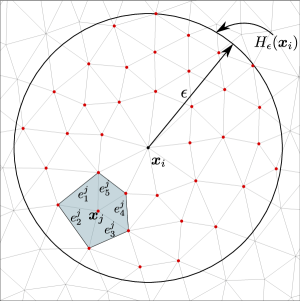
Figure 3: Typical mesh node $\boldsymbol{x}_{i}$ and one of the neighboring nodes $\boldsymbol{x}_{j}$ in an example 2-d finite element mesh. All the red nodes are the ones contributing to the force at $\boldsymbol{x}_{i}$. The set $E_{j}=\{e^{j}_{k}\}_{k=1}^{5}$ of elements with the node $\boldsymbol{x}_{j}$ as the vertex is shown in the grey region.

Algorithm 1 NFEA implementation

1:Read nodes and element-node connectivity from the mesh file

2:$\%\%$ Task: Create neighbor list and compute $V_{ij}$ using (62)

3:for Each integer $0\leq i\leq N-1$ do $\%$ $N$ is the total number of nodes

4:   if $|\boldsymbol{X}[i]-\boldsymbol{X}[j]|\leq\epsilon$ then $\%$ $\boldsymbol{X}$ - vector of reference coordinates of nodes

5:      Add $j$ to neighborList$[i]$

6:      Compute $V_{ij}$ using (62), add $V_{ij}$ to $V[i]$

7:   end if

8:end for$\>\%$ End of loop over nodes for neighborlist

9:$\%\%$ Task: Integrate in time

10:for Each integer $0\leq k\leq T/\Delta t$ do

11:   $\%$ $\boldsymbol{U},\boldsymbol{V}$ are the displacement and velocity at step $k$

12:   $\%\%$ Task: Compute force $\boldsymbol{F}$ using (63)

13:   Initialize vector $\boldsymbol{F}$ with zeros

14:   for Each integer $0\leq i\leq N-1$ do

15:      for Each integer $j\in$ neighborList$[i]$ do

16:         $S_{-}{ji}=\frac{\boldsymbol{U}[j]-\boldsymbol{U}[i]}{|\boldsymbol{X}[j]-\boldsymbol{X}[i]|}\cdot\frac{\boldsymbol{X}[j]-\boldsymbol{X}[i]}{|\boldsymbol{X}[j]-\boldsymbol{X}[i]|}$

17:         $\boldsymbol{F}[i]=\boldsymbol{F}[i]+\frac{\omega(\boldsymbol{X}[i])\omega(\boldsymbol{X}[j])}{\omega_{d}\epsilon^{d+1}}\,\psi^{\prime}(|\boldsymbol{X}[j]-\boldsymbol{X}[i]|\,S_{-}{ji}^{2})\,S_{-}{ji}\,\frac{\boldsymbol{X}[j]-\boldsymbol{X}[i]}{|\boldsymbol{X}[j]-\boldsymbol{X}[i]|}\,V[i][j]$

18:      end for

19:   end for$\>\%$ End of loop over nodes for $\boldsymbol{F}$

20:   $\%\%$ Task: Update displacement $\boldsymbol{U}$ and velocity $\boldsymbol{V}$

21:   for Each integer $0\leq i\leq N-1$ do

22:      for Each integer $0\leq l\leq d-i$ do $\%$ $d$ is the dimension of the problem

23:         $\boldsymbol{U}_{-}{temp}=\boldsymbol{U}[i][l]$

24:         if dof $l$ of node $i$ is free then

25:            $\boldsymbol{U}[i][l]=\boldsymbol{U}[i][l]+\Delta t\,\boldsymbol{V}[i][l]+\Delta t^{2}\frac{\boldsymbol{F}[i][l]+\boldsymbol{b}_{-}{l}(\boldsymbol{X}[i],k\Delta t)}{\rho(\boldsymbol{X}[i])}$

26:         else

27:            Read $\boldsymbol{U}[i][l]$ from boundary condition

28:         end if

29:         $\boldsymbol{V}[i][l]=\frac{\boldsymbol{U}[i][l]-\boldsymbol{U}_{-}{temp}[i][l]}{\Delta t}$

30:      end for

31:   end for$\>\%$ End of loop over nodes for $\boldsymbol{U}$ and $\boldsymbol{V}$ update

32:end for$\>\%$ End of loop over time

5.2 Material properties

For a given density $\rho$, Young’s modulus $E$, and critical energy release rate $G_{c}$, the material parameters for the PMB model (in 2-d), see (6), is given by

$$c=\frac{72E}{2\pi\epsilon^{3}},\quad S_{c}=\sqrt{\frac{5\pi G_{c}}{9E\epsilon}}.$$

The influence function is taken to be $J^{\epsilon}(r)=J(r/\epsilon)$, where $J(r)=1-r$ for $0\leq r<1$ and $J(r)=0$ for $r\geq 1$. The above set of relations are the same as in Bobaru and Hu, (2012).

Remark 5.1

It should be noted that the bond-based peridynamics suffer from the restriction of Poisson ratio $\nu=1/4$ in 3-d or 2-d plane strain and $\nu=1/3$ in 2-d plane stress; see Trageser and Seleson, (2020). All of our simulations are in 2-d, and plane strain is assumed. Therefore, $\nu$ is fixed to $1/4$.

Given $E$, $G_{c}$, and $\nu=1/4$, the critical stress intensity factor $K_{Ic}$ can be computed using the relation:

$$K_{Ic}=\sqrt{\frac{EG_{c}}{1-\nu^{2}}}=\sqrt{\frac{16EG_{c}}{15}}.$$

For the RNP model, see (9), the nonlinear potential function $\psi$ is fixed to $\psi(r)=c(1-\exp[-\beta r])$, where $c$ and $\beta$ are two parameters that will be fixed shortly. The influence function $J^{\epsilon}$ is the same as in the case of the PMB model. The boundary function $\omega(\boldsymbol{x})$ is taken as $1$ for all points $\boldsymbol{x}$ in the domain, i.e., $\omega(\boldsymbol{x})=1$ for $\boldsymbol{x}\in D$. Given $E$, Lamé parameter are $\lambda=\mu=2E/5$ ($\nu=1/4$ is assumed). The parameters $c$ and $\beta$, in 2-d, can be determined from (see Lipton, (2016))

$$c=\frac{G_{c}\pi}{4M_{J}},\quad\beta=\frac{8E}{5cM_{J}},$$ (64)

where, $M_{J}=\int_{0}^{1}J(r)r^{2}dr=1/12$ for $J(r)=1-r$. The inflection point of the potential function $\psi$ is given by $r^{\ast}=1/\sqrt{2\beta}$ and the critical strain $S_{c}(\boldsymbol{y},\boldsymbol{x})=\pm r^{\ast}/\sqrt{|\boldsymbol{y}-\boldsymbol{x}|}$.

Let $c_{L}$, $c_{S}$, and $c_{R}$ are the longitudinal, shear, and Rayleigh wave speeds, respectively. Given elastic properties such as $E$ and $\nu$, wave speeds can be computed as follows:

$$\begin{split}c_{L}&=\sqrt{\frac{\lambda+2\mu}{\rho}}=\sqrt{\frac{1}{\rho}\frac{E(1-\nu)}{(1+\nu)(1-2\nu)}},\quad c_{S}=\sqrt{\frac{\mu}{\rho}}=\sqrt{\frac{1}{\rho}\frac{E}{2(1+\nu)}},\quad c_{R}\approx c_{S}\left(\frac{0.862+1.14\nu}{1+\nu}\right),\end{split}$$ (65)

where the last formula to approximate Rayleigh wave speed can be found in Royer and Clorennec, (2007).

Material properties employed in numerical experiments are listed in Table 1.

Properties	Values		Properties	Values
$\rho$ $(kg/m^{3})$	$1200$		$c_{L}$ $(m/s)$	$6123.7$
$E$ $(GPa)$	$37.5$		$c_{S}$ $(m/s)$	$3535.5$
$G_{c}$ $(J/m^{2})$	$500$		$c_{R}$ $(m/s)$	$3244.2$

Table 1: Material properties. Here, following Remark 5.1, the Poisson ratio is $\nu=1/4$. Therefore, elastic properties, such as bulk and shear modulus and Lamè parameters, can be computed using the pair $(E,\nu)$. Further, using $E,G_{c},\nu$, $K_{Ic}$ can be computed using $K_{Ic}=\sqrt{\frac{EG_{c}}{1-\nu^{2}}}$. Formulas in (65) are used to compute longitudinal ($c_{L}$), shear ($c_{S}$), and Rayleigh ($c_{R}$) wave speeds.

Definition 5.2 (Damage)

The extent of damage at the material point $\boldsymbol{x}$ can be defined as

$$Z(\boldsymbol{x}):=\sup_{\boldsymbol{y}\in H_{\epsilon}(\boldsymbol{x})\cap D}\frac{|S(\boldsymbol{y},\boldsymbol{x})|}{|S_{c}(\boldsymbol{y},\boldsymbol{x})|}.$$ (66)

Based on the above, if $Z(\boldsymbol{x})\geq 1$, it follows that $\boldsymbol{x}$ has at least one bond in the neighborhood with the bond strain above the critical bond strain. The damage zone of the material is given by the set $\{\boldsymbol{x}\in D:Z(\boldsymbol{x})\geq 1\}$.

5.3 Mode-I crack propagation

Consider a square domain $D=[0,100\,\text{mm}]^{2}$ with a vertical pre-crack of length $l=20\,$mm at the center; see Fig. 4(a)(a). The constant velocity of $\pm 10^{3}$ mm/s is specified on the small area on the left and right sides to obtain the mode-I crack propagation. The simulation time and the size of the time step are $T=40\,\mu$s and $\Delta t=0.0008\,\mu$s, respectively. The nonlocal length-scale, i.e., horizon, is fixed to $\epsilon=2\,$mm. In the simulations, the RNP model with the material properties listed in Table 1 is employed.

First, the numerical convergence as the mesh is refined is analyzed for the mode-I crack propagation problem. Towards this, the simulations are carried out with three different mesh sizes $h_{1}=0.5,h_{2}=h_{1}/r,h_{3}=h_{2}/r$ mm with $r=2$, and the following formula is used to estimate the rate of convergence $\alpha(t^{k})$ at the $k^{\text{th}}$ time step in the $L^{2}$ norm:

$$\alpha(t^{k})=\frac{\log\left(||\boldsymbol{u}^{k}_{h_{1}}-\boldsymbol{u}^{k}_{h_{2}}||\right)-\log\left(||\boldsymbol{u}^{k}_{h_{2}}-\boldsymbol{u}^{k}_{h_{3}}||\right)}{\log(r)},$$ (67)

where $\boldsymbol{u}^{k}_{h_{i}}$ is the numerical solution at $k^{\text{th}}$ time step corresponding to the mesh with mesh size $h_{i}$. From Fig. 4(b), it is seen that the rate is below $2$. Based on earlier work Jha and Lipton, 2018b ; Jha and Lipton, 2018a ; Jha and Lipton, (2019), there are various factors that could lead to a sub-optimal rate of convergence, such as (1) $r=h_{1}/h_{2}=h_{2}/h_{3}$ must be much larger so that the relation $||\boldsymbol{u}^{k}_{h_{1}}-\boldsymbol{u}^{k}_{h_{2}}||=Ch_{1}^{\alpha}$ used to obtain an estimate of rate $\alpha$ from (67) is accurate and (2) ratio of the horizon to mesh size must also be large to minimize the inaccuracies in nonlocal integration and artifacts at the boundary of integral (elements partially inside the horizon).

Next, the plot of damage function $Z$ defined in (66) is shown in the left column of Fig. 5. In the right column, classical linearized strain is computed from the displacement field, and its magnitude (magnitude of the strain tensor $\boldsymbol{E}=\frac{1}{2}\left[\nabla\boldsymbol{u}+\nabla\boldsymbol{u}^{T}\right]$ is taken as $||\boldsymbol{E}||=\sqrt{\boldsymbol{E}\boldsymbol{:}\boldsymbol{E}}$, where $\boldsymbol{E}\boldsymbol{:}\boldsymbol{E}=E_{ij}E_{ij}$ is the dot product) is shown. In all the numerical results, it is found that the width of the process zone (damaged region) is approximately twice the horizon and envelopes the crack interface. Further, the strain tensor magnitude is unusually higher at the crack interface, as expected.

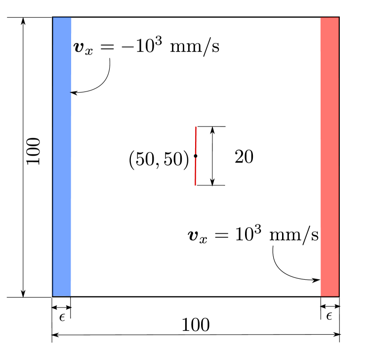
(a)

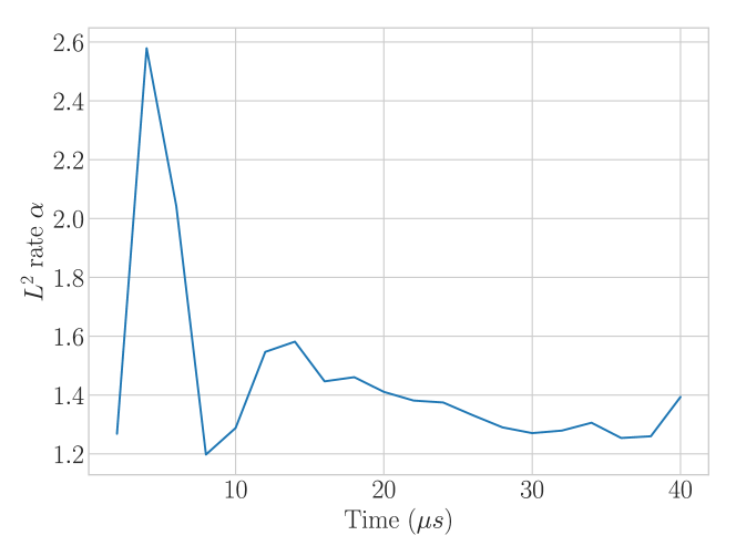
(b)

Figure 4: (a) Mode-I crack problem: Setup. The horizon is $\epsilon=2\,mm$. The center of the pre-crack coincides with the center of the domain. (b) Mode-I crack problem: Convergence rate as the mesh is refined.

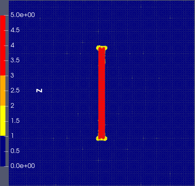
(c) $Z$ at $t=30\,\mu$s.

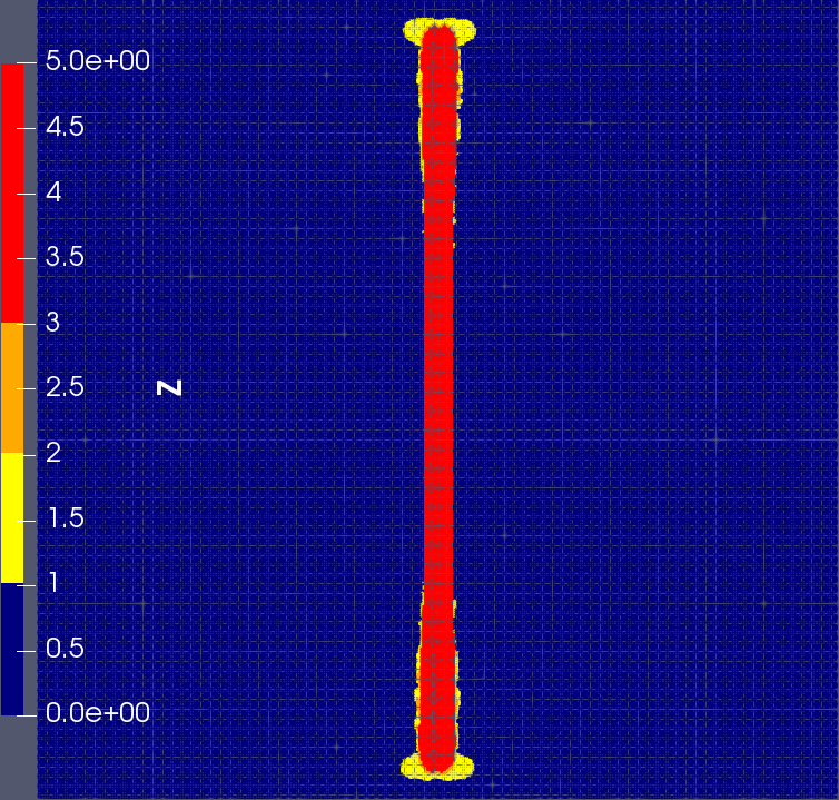
(d) Magnitude of strain at $t=30\,\mu$s.

(e) $Z$ at $t=38\,\mu$s.

(f) Magnitude of strain at $t=38\,\mu$s.

Figure 5: Mode-I crack problem: Plot of damage and the magnitude of the strain $\boldsymbol{E}=\frac{1}{2}\left[\nabla\boldsymbol{u}+\nabla\boldsymbol{u}^{T}\right]$. The damage and strains are localized near the crack interface. The thickness of the damage zone in the left column (red region) is approximately twice the horizon.

5.4 Material with a circular hole subjected to an axial loading

A material with a hole, as shown in Fig. 6, is subjected to displacement-controlled axial pulling. The details of the setup and boundary conditions are described in Fig. 6. The remaining parameters are fixed as follows: horizon $\epsilon=1$ mm, mesh size $h=0.25$ mm, final time of the simulation $T=160\,\mu$s, and the size of the time step $\Delta t=0.0016\,\mu$s. Peridynamics force is computed using the RNP model.

The damage profile and the strains are shown in Fig. 7. After the load reaches a sufficiently high value, the crack nucleation is observed. It is also clear that the crack nucleates at the top and bottom edges of the void where the strain is maximum (so stress is maximum). Branching of the cracks is also seen at later times.

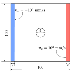
Figure 6: Circular hole problem: Setup. The horizon is $\epsilon=1$ mm. Constant velocity in the opposite direction is specified along the x-axis in the left (blue) and right (red) layers.

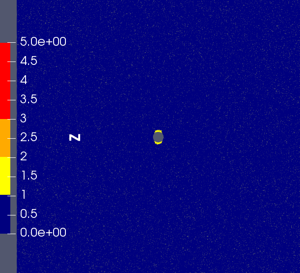
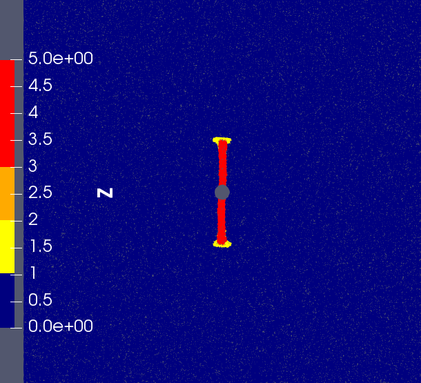
(a) $Z$ at $t=40\,\mu$s.

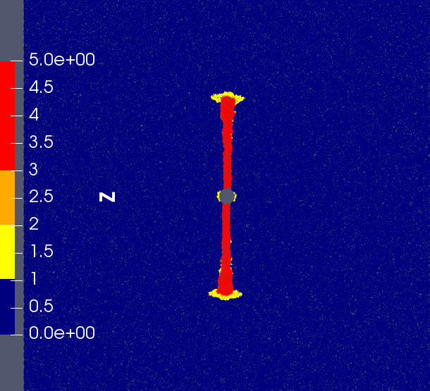
(b) $Z$ at $t=48\,\mu$s.

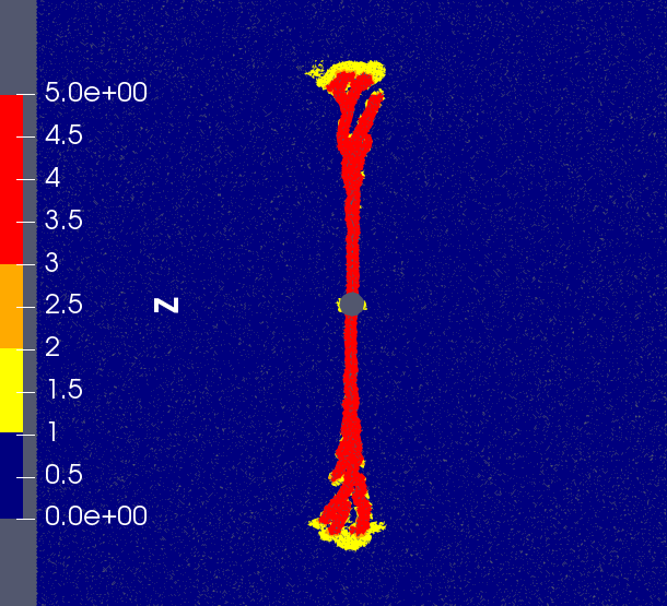
(c) $Z$ at $t=52\,\mu$s.

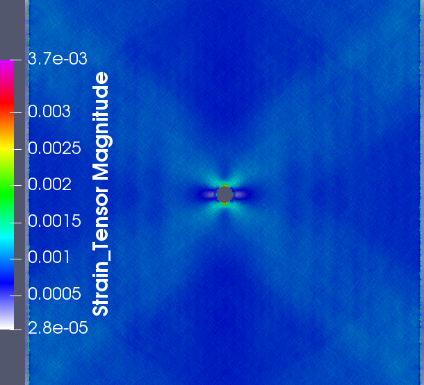
(d) $Z$ at $t=56\,\mu$s.

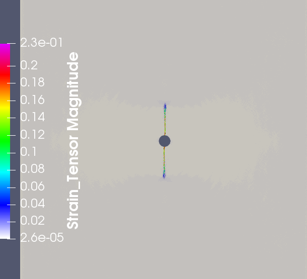
(e) Magnitude of strain at $t=40\,\mu$s.

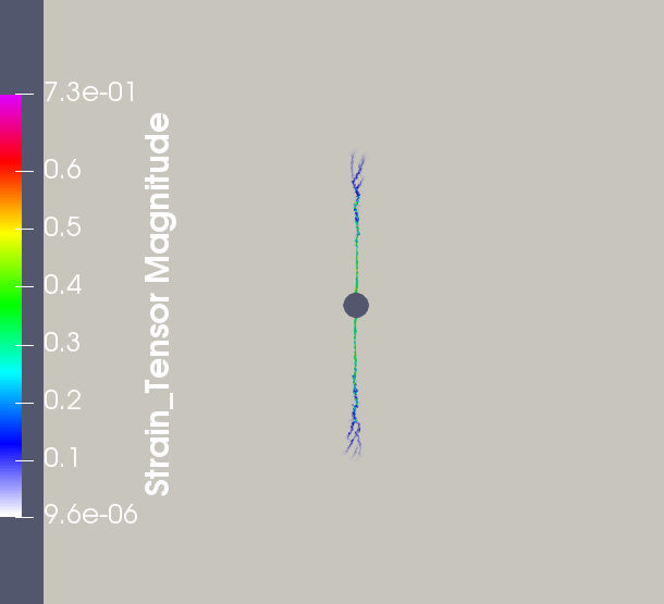
(f) Magnitude of strain at $t=48\,\mu$s.

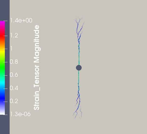
(g) Magnitude of strain at $t=52\,\mu$s.

(h) Magnitude of strain at $t=56\,\mu$s.

Figure 7: Circular hole problem: Plot of damage and the magnitude of the strain. A crack is seen nucleating at the two points on the edge of a hole where the strain is maximum.

5.5 Material with a v-notch under bending load

In this example, a specimen with a v-notch is subjected to the bending load as shown in Fig. 8. The horizon is fixed to $\epsilon=1$ mm, mesh size $h=0.25$ mm, final simulation time $T=250\,\mu$s, and the size of the time step $\Delta t=0.001667\,\mu$s. Peridynamics force is based on the RNP model.

The damage profile and the magnitude of the strain are plotted in Fig. 9. As expected, the crack nucleates at the tip of the notch where the strain is larger.

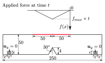
Figure 8: V-notch problem: Setup. The horizon in this problem is $\epsilon=1$ mm. Vertically downward distributed force is applied on the part of the top edge, as shown in red. The profile of distributed load is shown above the red line, where the loading parameter $f_{max}$ is set to $f_{max}=2.5\times 10^{11}$ N/(s$\cdot$mm).

(a) $Z$ at $t=150\,\mu$s.

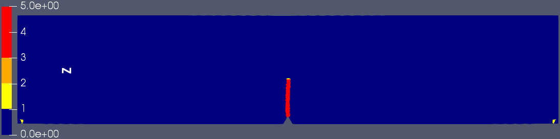
(b) Magnitude of strain at $t=150\,\mu$s.

(c) $Z$ at $t=175\,\mu$s.

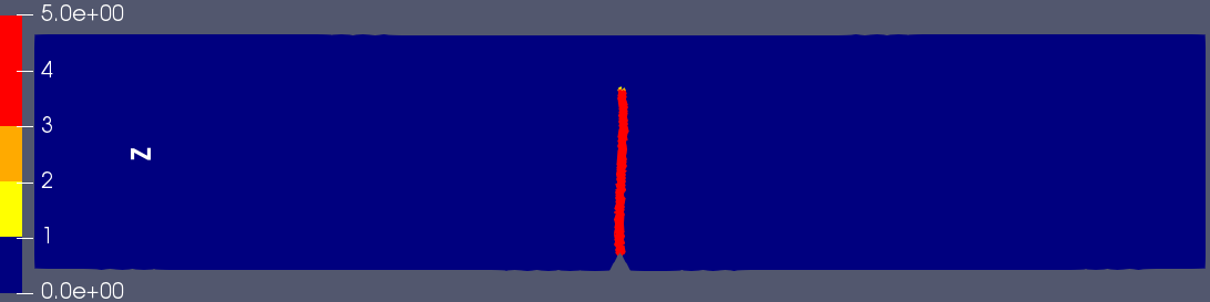
(d) Magnitude of strain at $t=175\,\mu$s.

(e) $Z$ at $t=200\,\mu$s.

(f) Magnitude of strain at $t=200\,\mu$s.

Figure 9: V-notch problem: Plot of damage and the magnitude of the strain. Crack nucleates at the tip of the notch where the strain is maximum.

5.6 Material with a circular hole and pre-crack

Consider a rectangular domain with existing horizontal pre-crack and a circular hole in the neighborhood of a crack as shown in Fig. 10. The horizon is fixed to $\epsilon=0.4$ mm, mesh size $h=0.1$ mm, the final simulation time $T=800\,\mu$s, and the size of the time step $\Delta t=0.004\,\mu$s. The peridynamics force is computed using the RNP model.

Damage and the magnitude of the strain at different times are shown in Fig. 11. Initially, crack propagation is influenced by the hole nearby, and instead of growing horizontally, it is deflected. At later times, when the hole is past the crack tip, the crack propagates horizontally as expected. A similar problem was considered in [Figure 18, Dai et al., (2015)], where results using different numerical methods were compared. The results of this work qualitatively agree with that in Dai et al., (2015).

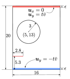
Figure 10: Circular hole and pre-crack problem: Setup. The horizon is $\epsilon=0.4$ mm. The magnitude of the prescribed vertical velocity on the top and bottom layers is $\bar{v}=25$ mm/s.

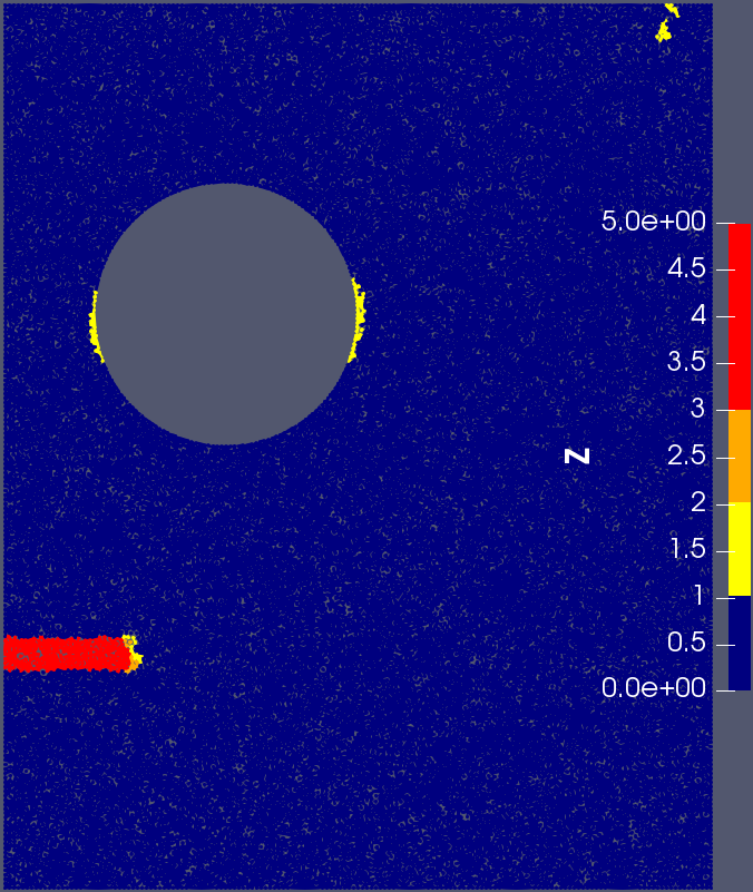
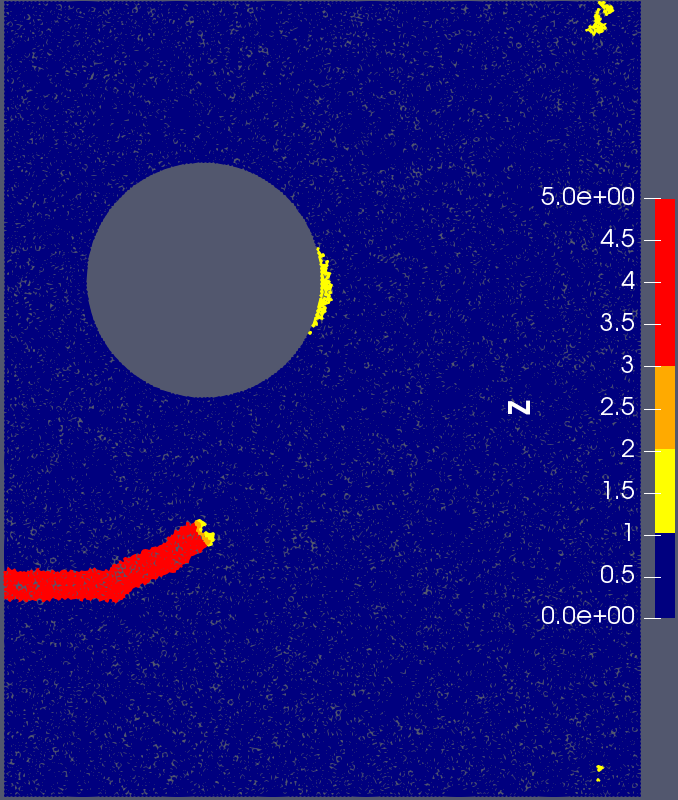
(a) $t=448\,\mu$s.

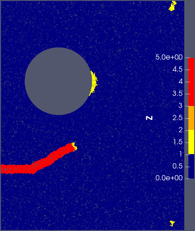
(b) $t=480\,\mu$s.

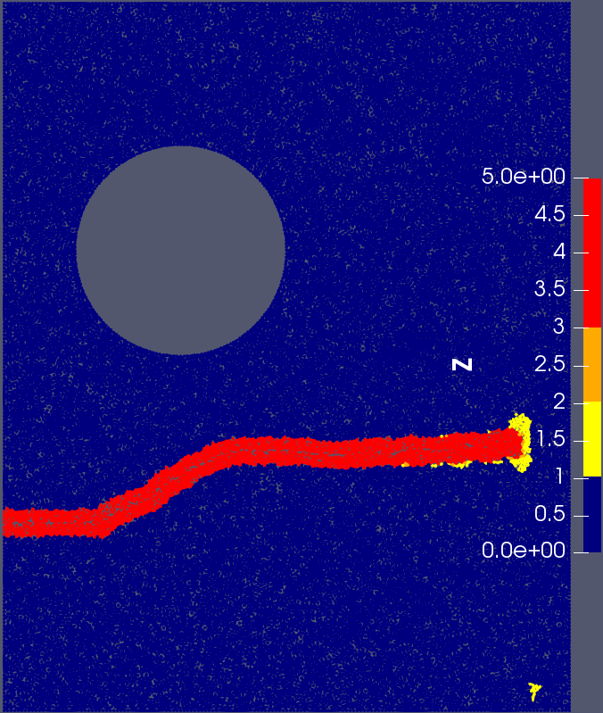
(c) $t=528\,\mu$s.

(d) $t=536\,\mu$s.

Figure 11: Circular hole and pre-crack problem: Plot of damage.

(a) $t=448\,\mu$s.

(b) $t=480\,\mu$s.

(c) $t=528\,\mu$s.

(d) $t=536\,\mu$s.

Figure 12: Circular hole and pre-crack problem: Plot of the magnitude of strain $\boldsymbol{E}=\frac{1}{2}\left[\nabla\boldsymbol{u}+\nabla\boldsymbol{u}^{T}\right]$.

5.7 On the crack propagation speed

In this subsection, the speed of the crack propagation in all four problems is compared. Let $t_{1}$ and $t_{2}$ be times when the crack begins and stops propagating, respectively. Also, let $v(t)$, for $t\in[t_{1},t_{2}]$, be the crack speed computed from the simulation at time $t$. To plot the crack speeds for all four examples in one plot, time $t\in[t_{1},t_{2}]$ is transformed to $\bar{t}=(t-t_{1})/(t_{2}-t_{1})$ so that $\bar{t}\in[0,1]$. Let $\bar{v}(\bar{t})=v(t)$ be the crack speed as a function of normalized time $\bar{t}$. Next, crack speed is normalized by dividing the Rayleigh wave speed $c_{R}$; $c_{R}$ from Table 1 is $3244.2$ m/s.

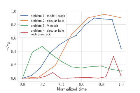
Figure 13: Comparison of the normalized crack speed for the four problems.

Problem type	$\max\left(\frac{v}{c_{R}}\right)$	$\mathrm{avg}\left(\frac{v}{c_{R}}\right)$		Problem type	$\max\left(\frac{v}{c_{R}}\right)$	$\mathrm{avg}\left(\frac{v}{c_{R}}\right)$
Mode-I crack	0.9	0.51		Circular hole	0.95	0.52
V-notch	0.47	0.22		Circular hole with pre-crack	0.32	0.04

Table 2: Maximum and average normalized crack speeds for the four numerical problems.

Fig. 13 presents the normalized crack speed as a function of normalized time for the four problems. As expected, the normalized crack speeds are below 1, i.e., the crack propagates slower than the Rayleigh wave speed; see Table 2, which lists the maximum and average values of normalized crack speeds.

6 Conclusion

This work analyzed the nodal finite element approximation for the peridynamics. Assuming exact solutions are in proper function spaces, consistency errors are shown to be bounded, and a-priori convergence of the discretization is established. The implementation of the nodal finite element discretization is discussed in detail, and a range of numerical experiments are performed using the method to show the utility of the approximation. The nodal finite element approximation is relatively straightforward to implement and can be easily integrated with the standard finite element meshing libraries. Further, the method is computationally faster than the standard finite element approximation due to the fact that the mass matrix is diagonal and the nonlocal force calculation is similar to finite-difference/mesh-free approximation.

References

- Agwai et al., (2011) Agwai, A., Guven, I., and Madenci, E. (2011). Predicting crack propagation with peridynamics: a comparative study. International journal of fracture, 171(1):65–78.
- Ahrens et al., (2005) Ahrens, J., Geveci, B., and Law, C. (2005). Paraview: An end-user tool for large data visualization. The visualization handbook, 717.
- Aksoylu and Unlu, (2014) Aksoylu, B. and Unlu, Z. (2014). Conditioning analysis of nonlocal integral operators in fractional sobolev spaces. SIAM Journal on Numerical Analysis, 52:653–677.
- Anicode and Madenci, (2022) Anicode, S. V. K. and Madenci, E. (2022). Bond-and state-based peridynamic analysis in a commercial finite element framework with native elements. Computer Methods in Applied Mechanics and Engineering, 398:115208.
- Bobaru and Hu, (2012) Bobaru, F. and Hu, W. (2012). The meaning, selection, and use of the peridynamic horizon and its relation to crack branching in brittle materials. International journal of fracture, 176(2):215–222.
- Brenner and Scott, (2007) Brenner, S. and Scott, R. (2007). The mathematical theory of finite element methods, volume 15. Springer Science & Business Media, 3 edition.
- Chen and Gunzburger, (2011) Chen, X. and Gunzburger, M. (2011). Continuous and discontinuous finite element methods for a peridynamics model of mechanics. Computer Methods in Applied Mechanics and Engineering, 200(9-12):1237–1250.
- Dai et al., (2015) Dai, S., Augarde, C., Du, C., and Chen, D. (2015). A fully automatic polygon scaled boundary finite element method for modelling crack propagation. Engineering Fracture Mechanics, 133:163–178.
- De Meo and Oterkus, (2017) De Meo, D. and Oterkus, E. (2017). Finite element implementation of a peridynamic pitting corrosion damage model. Ocean Engineering, 135:76–83.
- Diehl et al., (2020) Diehl, P., Jha, P. K., Kaiser, H., Lipton, R., and Lévesque, M. (2020). An asynchronous and task-based implementation of peridynamics utilizing hpx—the c++ standard library for parallelism and concurrency. SN Applied Sciences, 2(12):1–21.
- Diehl et al., (2022) Diehl, P., Lipton, R., Wick, T., and Tyagi, M. (2022). A comparative review of peridynamics and phase-field models for engineering fracture mechanics. Computational Mechanics, 69(6):1259–1293.
- Diehl et al., (2019) Diehl, P., Prudhomme, S., and Lévesque, M. (2019). A review of benchmark experiments for the validation of peridynamics models. Journal of Peridynamics and Nonlocal Modeling, 1:14–35.
- Diyaroglu et al., (2017) Diyaroglu, C., Oterkus, S., Oterkus, E., and Madenci, E. (2017). Peridynamic modeling of diffusion by using finite-element analysis. IEEE Transactions on Components, Packaging and Manufacturing Technology, 7(11):1823–1831.
- Du et al., (2018) Du, Q., Tao, Y., and Tian, X. (2018). A peridynamic model of fracture mechanics with bond-breaking. Journal of Elasticity, 132(2):197–218.
- Emmrich et al., (2013) Emmrich, E., Lehoucq, R. B., and Puhst, D. (2013). Peridynamics: a nonlocal continuum theory. In Meshfree Methods for Partial Differential Equations VI, pages 45–65. Springer.
- Foster et al., (2011) Foster, J. T., Silling, S. A., and Chen, W. (2011). An energy based failure criterion for use with peridynamic states. International Journal for Multiscale Computational Engineering, 9(6).
- Geuzaine and Remacle, (2009) Geuzaine, C. and Remacle, J.-F. (2009). Gmsh: A 3-d finite element mesh generator with built-in pre-and post-processing facilities. International journal for numerical methods in engineering, 79(11):1309–1331.
- Ghajari et al., (2014) Ghajari, M., Iannucci, L., and Curtis, P. (2014). A peridynamic material model for the analysis of dynamic crack propagation in orthotropic media. Computer Methods in Applied Mechanics and Engineering, 276:431–452.
- Ha and Bobaru, (2010) Ha, Y. D. and Bobaru, F. (2010). Studies of dynamic crack propagation and crack branching with peridynamics. International Journal of Fracture, 162(1-2):229–244.
- Heller et al., (2017) Heller, T., Diehl, P., Byerly, Z., Biddiscombe, J., and Kaiser, H. (2017). HPX – An open source C++ Standard Library for Parallelism and Concurrency. In Proceedings of OpenSuCo 2017, Denver , Colorado USA, November 2017 (OpenSuCo’17), page 5.
- Huang et al., (2019) Huang, X., Bie, Z., Wang, L., Jin, Y., Liu, X., Su, G., and He, X. (2019). Finite element method of bond-based peridynamics and its abaqus implementation. Engineering Fracture Mechanics, 206:408–426.
- Jha and Lipton, (2021) Jha, P. and Lipton, R. (2021). Finite element approximation of nonlocal dynamic fracture models. Discrete & Continuous Dynamical Systems-B, 26(3):1675.
- Jha et al., (2021) Jha, P. K., Desai, P. S., Bhattacharya, D., and Lipton, R. (2021). Peridynamics-based discrete element method (peridem) model of granular systems involving breakage of arbitrarily shaped particles. Journal of the Mechanics and Physics of Solids, 151:104376.
- Jha and Diehl, (2021) Jha, P. K. and Diehl, P. (2021). Nlmech: Implementation of finite difference/meshfree discretization of nonlocal fracture models. Journal of Open Source Software, 6(65):3020.
- (25) Jha, P. K. and Lipton, R. (2018a). Numerical analysis of nonlocal fracture models in holder space. SIAM Journal on Numerical Analysis, 56(2):906–941.
- (26) Jha, P. K. and Lipton, R. (2018b). Numerical convergence of nonlinear nonlocal continuum models to local elastodynamics. International Journal for Numerical Methods in Engineering, 114(13):1389–1410.
- Jha and Lipton, (2019) Jha, P. K. and Lipton, R. (2019). Numerical convergence of finite difference approximations for state based peridynamic fracture models. Computer Methods in Applied Mechanics and Engineering, 351:184–225.
- (28) Jha, P. K. and Lipton, R. (2020a). Finite element convergence for state-based peridynamic fracture models. Communications on Applied Mathematics and Computation, 2(1):93–128.
- (29) Jha, P. K. and Lipton, R. P. (2020b). Kinetic relations and local energy balance for lefm from a nonlocal peridynamic model. International Journal of Fracture.
- Kaiser et al., (2018) Kaiser, H., aka wash, B. A. L., Heller, T., Bergé, A., Biddiscombe, J., Simberg, M., Bikineev, A., Mercer, G., Schäfer, A., Serio, A., Kwon, T., George, A. V., Habraken, J., Anderson, M., Copik, M., Brandt, S. R., Huck, K., Stumpf, M., Bourgeois, D., Blank, D., Jakobovits, S., Amatya, V., Viklund, L., Khatami, Z., Bacharwar, D., Yang, S., Schnetter, E., Bcorde5, Christopher, and Brodowicz, M. (2018). STEllAR-GROUP/hpx: HPX V1.1.0: The C++ Standards Library for Parallelism and Concurrency.
- Kaiser et al., (2020) Kaiser, H., Diehl, P., Lemoine, A. S., Lelbach, B. A., Amini, P., Berge, A., Biddiscombe, J., Brandt, S. R., Gupta, N., Heller, T., Huck, K., Khatami, Z., Kheirkhahan, A., Reverdell, A., Shirzad, S., Simberg, M., Wagle, B., Wei, W., and Zhang, T. (2020). Hpx - the c++ standard library for parallelism and concurrency. Journal of Open Source Software, 5(53):2352.
- Lipton, (2014) Lipton, R. (2014). Dynamic brittle fracture as a small horizon limit of peridynamics. Journal of Elasticity, 117(1):21–50.
- Lipton, (2016) Lipton, R. (2016). Cohesive dynamics and brittle fracture. Journal of Elasticity, 124(2):143–191.
- Lipton et al., (2016) Lipton, R., Silling, S., and Lehoucq, R. (2016). Complex fracture nucleation and evolution with nonlocal elastodynamics. arXiv preprint arXiv:1602.00247.
- Lipton et al., (2019) Lipton, R. P., Lehoucq, R. B., and Jha, P. K. (2019). Complex fracture nucleation and evolution with nonlocal elastodynamics. Journal of Peridynamics and Nonlocal Modeling, 1(2):122–130.
- Macek and Silling, (2007) Macek, R. W. and Silling, S. A. (2007). Peridynamics via finite element analysis. Finite Elements in Analysis and Design, 43(15):1169–1178.
- Madenci et al., (2018) Madenci, E., Dorduncu, M., Barut, A., and Phan, N. (2018). A state-based peridynamic analysis in a finite element framework. Engineering Fracture Mechanics, 195:104–128.
- Mengesha and Du, (2015) Mengesha, T. and Du, Q. (2015). On the variational limit of a class of nonlocal functionals related to peridynamics. Nonlinearity, 28(11):3999.
- Ni et al., (2018) Ni, T., Zhu, Q.-z., Zhao, L.-Y., and Li, P.-F. (2018). Peridynamic simulation of fracture in quasi brittle solids using irregular finite element mesh. Engineering Fracture Mechanics, 188:320–343.
- Royer and Clorennec, (2007) Royer, D. and Clorennec, D. (2007). An improved approximation for the rayleigh wave equation. Ultrasonics, 46(1):23–24.
- Silling et al., (2010) Silling, S., Weckner, O., Askari, E., and Bobaru, F. (2010). Crack nucleation in a peridynamic solid. International Journal of Fracture, 162(1-2):219–227.
- Silling, (2000) Silling, S. A. (2000). Reformulation of elasticity theory for discontinuities and long-range forces. Journal of the Mechanics and Physics of Solids, 48(1):175–209.
- Silling and Bobaru, (2005) Silling, S. A. and Bobaru, F. (2005). Peridynamic modeling of membranes and fibers. International Journal of Non-Linear Mechanics, 40(2):395–409.
- Silling et al., (2007) Silling, S. A., Epton, M., Weckner, O., Xu, J., and Askari, E. (2007). Peridynamic states and constitutive modeling. Journal of Elasticity, 88(2):151–184.
- Silling and Lehoucq, (2008) Silling, S. A. and Lehoucq, R. B. (2008). Convergence of peridynamics to classical elasticity theory. Journal of Elasticity, 93(1):13–37.
- Trageser and Seleson, (2020) Trageser, J. and Seleson, P. (2020). Bond-based peridynamics: A tale of two poisson’s ratios. Journal of Peridynamics and Nonlocal Modeling, 2(3):278–288.
- Weckner and Abeyaratne, (2005) Weckner, O. and Abeyaratne, R. (2005). The effect of long-range forces on the dynamics of a bar. Journal of the Mechanics and Physics of Solids, 53(3):705–728.
- Wildman et al., (2017) Wildman, R. A., O’Grady, J. T., and Gazonas, G. A. (2017). A hybrid multiscale finite element/peridynamics method. International Journal of Fracture, 207(1):41–53.
- Yang et al., (2019) Yang, Z., Oterkus, E., Nguyen, C. T., and Oterkus, S. (2019). Implementation of peridynamic beam and plate formulations in finite element framework. Continuum Mechanics and Thermodynamics, 31:301–315.