Absence of concordance in a simple self-interacting neutrino cosmology

Abstract

Some cosmic microwave background (CMB) data allow a cosmological scenario in which the free streaming of neutrinos is delayed until close to matter-radiation equality. Interestingly, recent analyses have revealed that large-scale structure (LSS) data also align with this scenario, discarding the possibility of an accidental feature in the CMB sky and calling for further investigation into the free-streaming nature of neutrinos. By assuming a simple representation of self-interacting neutrinos, we investigate whether this nonstandard scenario can accommodate a consistent cosmology for both the CMB power spectra and the large-scale distribution of galaxies simultaneously. Employing three different approaches — a profile likelihood exploration, a nested sampling method, and a heuristic Metropolis-Hasting approximation — we exhaustively explore the parameter space and demonstrate that galaxy data exacerbates the challenge already posed by the Planck polarization data for this nonstandard scenario. We find that the most conservative value of the Bayes factor disfavors the interactions among neutrinos over a $\Lambda$CDM + $N_{\mathrm{eff}}$ + $\sum m_{\nu}$ model with odds of $23:1000$ and that the difficulty of simultaneously fitting the galaxy and CMB data relates to the so-called $S_{8}$ discrepancy. Our analysis not only emphasizes the need to consider a broader range of phenomenologies in the early Universe but also highlights significant numerical and theoretical challenges ahead in uncovering the exact nature of the feature observed in the data or, ultimately, confirming the standard chronological evolution of the Universe.

I Introduction

Despite their weak interactions making them elusive, neutrinos significantly influence the intricate evolution of the Universe. Their gravitational interactions leave sizable imprints in various cosmological observables across different times and scales. These features contribute to unveiling the nature of neutrinos through cosmological observations, enabling tight constraints on pivotal parameters describing neutrino properties, such as the sum of neutrino masses, $\sum m_{\nu}$, and the effective number of relativistic species, $N_{\mathrm{eff}}$ [see Refs.  1, 2, 3, for instance]. Yet, cosmological phenomena could help us to achieve a more comprehensive and profound understanding of neutrino physics that extends beyond constraints on $\sum m_{\nu}$ and $N_{\mathrm{eff}}$.

Cosmology holds the potential to contribute to a better understanding of neutrino physics, as observables provide a path to test the free-streaming nature of neutrinos and, by extension, new physics in this sector. According to the Standard Model (SM), neutrinos decouple from the cosmic plasma and commence to free streaming as the Universe cools to approximately $\sim 1.5$ MeV. In the free-streaming phase, neutrinos remain gravitationally coupled, tugging any particles in their paths and leaving distinctive imprints on the evolution of cosmological perturbations [4]. New physics in the neutrino sector, however, can significantly alter these imprints [see Ref. 5, for instance].

In this context, novel neutrino interactions have been employed to investigate how altering the neutrino free streaming impacts the cosmological observables [see Refs.  6, 7, 8, 9, 10, 11, 12, 13, 14, 15, 16, 17, 18, 19, 20, 21, 22, 23, 24, 25, 26, 27, 28, 29, 30, 31, 32, 33, 34, 35, 36, 37, 38, 39, 40, 41, 42, 43, 44, 45, 46, 47, 48, 49, 50, 51, 52, 53, 54, 55, 56, 57, 58, 59, 60, 61, for instance]. In the last decade, analyses of cosmological scenarios with self-interacting neutrinos have shown that some data not only agree with a paradigm allowing moderate interactions among neutrinos (MI$\nu$) — effectively recovering the SM limit — but also with a radical scenario where strong interactions among neutrinos delay their free streaming until close to matter-radiation equality (SI$\nu$) [9, 10, 11, 12, 16, 38, 23, 40, 49, 28, 29, 58, 59]. Although these divergent pictures were initially found in the cosmic microwave background (CMB), a recent CMB-independent analysis demonstrated that large-scale structure (LSS) observations also support the SI_ν scenario [62], discarding the presumption of an accidental feature in the CMB data (see also Ref. [63]) and increasing the riddle surrounding the free-streaming nature of neutrinos.

The intriguing aspect of the SI_ν mode is noteworthy not only because it could hint at new physics in the early Universe but also due to its markedly varying statistical significance in different cosmological data contexts. For instance, polarization data provided by Planck [1] largely disfavor this extreme scenario [38, 39, 40, 49]. In agreement with this, standard neutrino free streaming appear to be favored by the agreement found between the imprints predicted by the SM and the observed phase of both CMB peaks [64] and baryon acoustic oscillations (BAO) [65, 66]. In contrast, data from the Atacama Cosmology Telescope (ACT) [67] notably favors a delayed neutrino free streaming cosmology [58, 59], and more recently, an analysis of diverse cosmological data, including Lyman-$\alpha$ power spectrum from SDSS DR14 BOSS and eBOSS quasars [68], largely favors the SI_ν scenario [63].

Complementing this picture, our previous CMB-independent analysis [62] not only reveals a modest preference for a delayed onset of neutrino free streaming but also indicates a comparable phenomenology to that observed in the CMB data. Both data exhibit similarities in the self-interaction strength and important correlations between the neutrino interaction and the amplitude, $A_{\rm s}$, and tilt, $n_{\rm s}$, of the primordial curvature power spectrum. These similarities could suggest the existence of a self-consistent picture capable of providing a simultaneously good fit to the CMB and galaxy power spectra.

In this work, we investigate whether self-interacting neutrinos can provide a consistent cosmological scenario for both the CMB power spectra and the large-scale distribution of galaxies simultaneously. By adopting the simplest cosmological representation for self-interacting neutrinos, an effective four-fermion interaction model, and performing an exhaustive exploration of the parameter space considering three different statistical approaches — a profile likelihood exploration, a nested sampling method, and a heuristic Metropolis-Hasting approximation — we determine the statistical significance of the SI_ν scenario in light of the galaxy and CMB power spectra data. Our analyses robustly demonstrate that the inclusion of galaxy power spectra data diminishes the statistical significance of a strongly self-interacting neutrino cosmology, exacerbating the challenge already posed by the Planck polarization data. As detailed below, this reduction is mainly driven by a mild inconsistency between the CMB and LSS data. Additionally, we describe and discuss some of the numerical challenges encountered when exploring a radical non-standard cosmological scenario with state-of-the-art cosmological data.

This paper is organized as follows. In Sec. II, we present the framework used to model neutrino interactions and briefly review its impacts in the galaxy and CMB power spectra. The data and methodology used in this paper are presented in Sec. III, while our results and discussion are shown in Sec. IV. Finally, we conclude in Sec. V.

II A delayed free streaming scenario: self-interactions in the neutrino sector

According to the SM, neutrinos decouple from the primordial bath and commence to free stream when the temperature of the Universe drops to about $1.5$ MeV. Due to their gravitational coupling, the supersonic free-streaming neutrinos tug on any particles in their paths, leaving distinctive imprints on the cosmological perturbations [4]. However, novel interactions in the neutrino sector could alter this free-streaming pattern, affecting expected signatures in the cosmological phenomena. While the exact phenomenology of these interactions dictates specific alterations in neutrino free streaming, on the whole, self-interacting neutrinos do not contribute to the anisotropic stress of the Universe. Investigating scenarios involving self-interacting neutrinos that delay neutrino free streaming is thus of great significance, considering that free-streaming neutrinos are the exclusive source of anisotropic stress during early times. In this work, we adopt a simple self-interacting neutrino model to explore whether a cosmological scenario with a delayed neutrino free streaming can simultaneously fit the observed CMB and galaxy power spectra.

A delayed neutrino free streaming cosmological scenario can be achieved by the simplest representation of self-interacting neutrinos: an effective four-fermion interaction universally coupling to all neutrino species, characterized by a dimensionful Fermi-like constant, $G_{\mathrm{eff}}$, and interaction rate:

$$\Gamma\equiv aG^{2}_{\mathrm{eff}}T^{5}_{\nu}\,,$$ (1)

where $a$ is the scale factor and $T_{\nu}$ the temperature of neutrinos. This representation, which can be thought of as a Yukawa-type interaction between neutrinos and a scalar mediator particle, $\varphi$, of mass $m_{\varphi}\gtrsim 1$ keV, (see e.g. Ref. [69] for a review) serves as a proxy to assess the impact of a delayed neutrino free streaming in the evolution of cosmological perturbation. Yet, this scenario is unlikely to correspond to a realistic representation of non-standard neutrino interactions.

As discussed in previous papers [see 28, 62, for instance], the model adopted here faces stringent constraints beyond cosmology [70, 71, 72, 73, 74, 75, 76, 77, 78, 79, 80, 81, 82, 83, 84, 85, 86, 87, 88, 89, 90, 91, 92, 93, 94, 95, 96, 95, 96, 97, 98, 99, 100].When taken at face value, such constraints only allow interactions that barely delay the neutrino free streaming, leading to cosmological scenarios where observables remain unchangeable. Moreover, Planck polarization data largely disfavor this simple representation, featuring instead a preference for phenomenologies that include a flavor-dependent coupling [38, 39, 40, 49]. We employ this simple model, however, to provide an exhaustive joint analysis of the CMB and galaxy data. By limiting the complexity of the self-interaction model, we focus on broadly exploring the relevant parameter space. As discussed in the following sections, the cosmologies explored here significantly deviate from the standard paradigm and pose diverse challenges that complicate the analysis of the state-of-the-art cosmological data.

The impacts that self-interactions in the neutrino sector produce in the evolution of the Universe are particularly notable in the evolution of the cosmological perturbations. Given that the interactions among neutrinos suppress the exclusive source of anisotropic stress in the early Universe, perturbations crossing the horizon during the tight-coupling phase exhibit distinct behavior from those crossing after the onset of free streaming, inducing a rich scale-dependent phenomenology in the cosmological observables. These effects become observable in the linear and mildly nonlinear scales for sufficiently large values of the self-interaction strength $\log_{10}(G_{\mathrm{eff}}/\mathrm{MeV}^{-2})\gtrsim-4.5$.

Observationally, the presence of self-interactions in the neutrino sector increases the amplitude of the CMB power spectrum while also inducing a phase shift towards smaller scales — larger $\ell$. In the linear matter power spectrum, the delay on the onset of the neutrino free streaming yields conspicuous scale-dependent signatures. In particular, interactions among neutrinos yield a suppression (enhancement) of the linear power spectrum at scales that cross the horizon when neutrinos are tightly coupled (commence to free-streaming). For a more detailed description, see Ref. [62] and references therein.

We highlight that $G_{\mathrm{eff}}$ is given in units of MeV^-2, and that the usual Fermi constant corresponds to the value $G_{\mathrm{eff}}\sim\mathcal{O}(10^{-11})$ MeV^-2. In order to consider a broad phenomenology, besides using $\log_{10}(G_{\mathrm{eff}}/\mathrm{MeV}^{-2})$ to control the onset of neutrino free streaming, our model also considers the effective number of relativistic species, $N_{\mathrm{eff}}$, and the sum of neutrino masses, $\sum m_{\nu}$, as free parameters. For sake of simplicity, all models considered in this work assume a single massive neutrino containing all the mass instead of several degenerate massive neutrinos.

III Data and methodology

We perform cosmological analysis using our modified version of CLASS-PT [101, 102]  along with the montepython code [103, 104]. We exhaustively explore the parameter space using three different schemes: a profile likelihood approximation, a heuristic Metropolis-Hasting pooling method, and the nested sampling algorithm [105]. Besides being advised to ensure a proper sample of the expected multi-modal posterior, the nested sampling algorithm provides a way to assess the statistical significance of cosmological models through the Bayes evidence. Complementary to this, the Metropolis-Hasting pooling method introduced here proposes a heuristic route to cross-check posterior inference provided by nested sampling. On the other hand, the profile likelihood approach allows us to identify possible volume effects and better understand the goodness of fit of the model. Unless otherwise stated, we assume the proper uniform priors presented in Table 1.

Table 1: Prior ranges used in the analyses.

Parameter	Prior
$\log_{10}(G_{\mathrm{eff}}/\mathrm{MeV}^{-2})$	$[-5.5,0.5]$
$N_{\mathrm{eff}}$	$[2.013,5.013]$
$\sum m_{\nu}\left[\mathrm{eV}\right]$	$[0.06,1.5]$
$\omega_{\mathrm{b}}$	$[0.018,0.03]$
$\omega_{\mathrm{cdm}}$	$[0.1,0.2]$
$H_{0}\left[\mathrm{km\>s}^{-1}\mathrm{Mpc}^{-1}\right]$	$[60,80]$
$\ln(10^{10}A_{\rm s})$	$[2,4]$
$n_{\rm s}$	$[0.85,1.1]$
$\tau_{\mathrm{reio}}$	$[0.01,0.25]$

III.1 Profile likelihood

We profile the likelihood of $\log_{10}(G_{\mathrm{eff}}/\mathrm{MeV}^{-2})$ in twenty-four equally linearly spaced values distributed in $\log_{10}(G_{\mathrm{eff}}/\mathrm{MeV}^{-2})=[-5.5,0.5]$. In contrast to our earlier analysis [62], we observe that relying solely on a minimization algorithm for profiling the likelihood is highly inefficient when considering both CMB and galaxy power spectra observation simultaneously. Conversely, modified Metropolis-Hastings methods (as seen in Ref. [106]) may become computationally burdensome when applied to the twenty-four assumed value of $\log_{10}(G_{\mathrm{eff}}/\mathrm{MeV}^{-2})$. To overcome this issue, we employ a hybrid approach.

Starting with a prior $\log_{10}(G_{\mathrm{eff}}/\mathrm{MeV}^{-2})=[-2.5,0.5]$, we obtain an initial best-fit through a Metropolis-Hastings exploration, demanding $R-1\lesssim 0.25$ for all parameters, where $R$ represents the Gelman-Rubin estimator [107]. Employing this result as the initial input for the Derivative-Free Optimizer for Least-Squares (DFOLS) package [108], we then minimize the likelihood across the values in the range $\log_{10}(G_{\mathrm{eff}}/\mathrm{MeV}^{-2})=[-2.5,0.5]$, finding the corresponding best-fits. We repeat the same process for the remaining parameter space, i.e., considering the prior $\log_{10}(G_{\mathrm{eff}}/\mathrm{MeV}^{-2})=[-5.5,-2.5]$. This analysis produces a collection of discrete points outlining the profile likelihood along the parameter space of interest. In Sec. IV, we supplement this result with a smooth representation obtained through a cubic spline interpolation.

III.2 Nested sampling exploration

To determine the statistical significance of the cosmological scenarios analyzed here, we sample the parameter space using the nested sampling (NS) algorithm [105]. In particular, we employ PyMultiNest [109], a Python implementation of MultiNest [110, 111]. Our main analyses optimize for estimation of the Bayesian evidence by using 2000 live points, a sampling efficiency of 0.3, and a minimum precision of $0.05$ in log-evidence.

Although NS is suitable for our study, it is crucial to bear in mind that this algorithm has potential limitations that can affect the analysis. These limitations, extensively discussed in the literature [105, 112, 113, 114, 115, 116], depend on factors such as the NS configuration and the nature of the likelihood under scrutiny. Identifying or addressing such deficiencies often requires multiple runs, resulting in a significant increase in computational time and resources used in the analysis. Here, we evaluate the potential impact of such limitations in our analyses using a heuristic approach based on a Metropolis-Hasting method. This method, thoroughly described in the following section, primarily aims to assess the accuracy of the inference of the posterior provided by NS sampling. However, it can also help to identify potential biases in the estimation of the Bayesian evidence. When performing multiple runs is computationally feasible, however, we assess possible NS deficiencies conducting additional analyses with varied NS configurations. The results of such analyses are presented in Appendix A.

III.3 Metropolis-Hasting pooling

It is well-known that Metropolis-Hasting methods (MH) exhibit inefficiencies in sampling multi-modal posteriors. These inefficiencies primarily arise from their intrinsic incapacity to traverse low-probability regions separating different modes. While some adaptations of the MH algorithm, such as parallel tempering [117], seek to address this limitation, they often come at the cost of more likelihood evaluations or require fine-tuned configuration.

Here, we introduce a heuristic method to sample the anticipated multi-modal posterior. Our method relies on the fact that low-probability barriers can be overcome by independently sampling disconnected portions of the parameter space where modes are expected. While directly pooling these independent samples would lead to a spurious realization of the target posterior, we note that is possible to recover the underlying posterior with an appropriate re-weighting process. We have found that an adequate re-weight can be achieved by exploiting the fact that, under uniform priors, for each mode $i$, the point that maximizes the posterior and likelihood, $\hat{\theta}^{i}$, leads to a constant ratio across the different modes,

$$\mathcal{R}=\frac{\mathcal{P}(\hat{\theta}^{i})}{\mathcal{L}(d|\hat{\theta}^{i})}\,,$$ (2)

where $\mathcal{P}(\theta)$ is the posterior, $\mathcal{L}(d|\theta)$ the likelihood, $d$ a given dataset, and $\theta$ the set of cosmological parameters, such that $\theta=\left\{\theta_{0},\theta_{1},...,\theta_{n}\right\}$, with $n$ being the number of free parameters considered into the analysis.

While computing $\mathcal{R}$ requires an a priori knowledge of the posterior, in practice, MH enables an approximation to the posterior-likelihood ratio. Based on the fact that the number of effective samples in the neighborhood of the peak of the likelihood should be proportional to $\mathcal{P}(\hat{\theta}^{i})$, we can compute such a ratio for each mode:

$$\tilde{\mathcal{R}}^{i}=\sum_{\hat{\theta}^{i}-\epsilon^{i}<\theta^{i}<\hat{\theta}^{i}+\epsilon^{i}}\frac{\alpha_{i}w(\theta^{i})}{\mathcal{L}(d|\hat{\theta}^{i})}\,,$$ (3)

where $[\hat{\theta}^{i}-\epsilon^{i},\hat{\theta}^{i}+\epsilon^{i}]$ defines a region that approximates the neighborhood of the peak of the likelihood, $w(\theta^{i})$ is the weight of the MH sample, and $\alpha_{i}$ is a re-weighting factor to be determined. The appropriate re-weight of samples can then be obtained by arbitrarily fixing one of re-weighting factors, $\alpha_{j}=1$, to later demand $\tilde{\mathcal{R}}^{i}=\tilde{\mathcal{R}}^{j}$ for all the remaining modes $i\neq j$.

We highlight that, although our method does not require fine-tuning extra parameters, Eq (3) exhibits some arbitrariness owing to the loose definition of the region $\smash{[\hat{\theta}^{i}-\epsilon^{i},\hat{\theta}^{i}+\epsilon^{i}]}$. Such arbitrariness, however, can be overcome by pragmatically defining $\epsilon^{i}$. We adopt the Freedman-Diaconis rule [118] and define:

$$\epsilon^{i}_{j}=2\frac{\mathrm{IQR}(\theta^{i}_{j})}{\sqrt[3]{N}}\,,$$ (4)

where $N$ is the number of samples obtained for the corresponding mode and $\mathrm{IQR}$ is the so-called interquartile range. We apply Eq. (4) for all the pertinent parameters, but the one that drives the multi-modality, $\theta_{k}$, which is left unbounded, $\epsilon_{k}\rightarrow\infty$.

Our particularly choice of Eq. (4) is further discussed in Appendix B, where we also present two toy models mimicking the expected bi-modal behaviour of $\log_{10}(G_{\mathrm{eff}}/\mathrm{MeV}^{-2})$ posterior. The analyses of such models show that the MH pooling method can recover the target posterior with considerable precision.

Anticipating a bi-modality in $\log_{10}(G_{\mathrm{eff}}/\mathrm{MeV}^{-2})$, we apply the MH pooling method considering two separate regions of the parameter space, i.e., we sample the SI_ν and MI_ν modes using the priors $\log_{10}(G_{\mathrm{eff}}/\mathrm{MeV}^{-2})=[-2.5,0.5]$ and $\log_{10}(G_{\mathrm{eff}}/\mathrm{MeV}^{-2})=[-5.5,-2.5]$, respectively. The remaining cosmological parameters follow the priors described at the beginning of this section, see Table 1. We evaluate the convergence on the corresponding chains demanding $R-1\lesssim 0.005$ for all cosmological parameters. To avoid biases due to differences on the effective number of samples, we run chains with approximately the same length and consider normalized weights on Eq. (3).

III.4 Cosmological data

We perform cosmological analyses considering different combinations of galaxy power spectrum, CMB, and Baryon Acoustic Oscillation (BAO) data. Specifically, we employ:

1. $\mathrm{TT}$: low-$\ell$ and high-$\ell$ CMB temperature power spectrum from Planck 2018 [1].

2. $\mathrm{EE,TE}$: low-$\ell$ and high-$\ell$ CMB E-mode polarization and their temperature cross correlation from Planck 2018 [1].

3. FS: the multipoles of the galaxy power spectrum $P_{\ell}(k,z)$ $(\ell=0,2,4)$ [119, 120] and the real space power spectrum estimator $Q_{0}$ [121] obtained from the window-free galaxy power spectrum analyses [122, 119] of the BOSS-DR12 galaxy sample [123, 124, 125], at redshift $0.38$ and $0.61$ for the north and south Galactic cap. We adopt $k_{\mathrm{min}}=0.01\>h/\mathrm{Mpc}$ and $k_{\mathrm{max}}=0.2\>h/\mathrm{Mpc}$ for $P_{\ell}$ and $k_{\mathrm{min}}=0.2\>h/\mathrm{Mpc}$ and $k_{\mathrm{max}}=0.4\>h/\mathrm{Mpc}$ for $Q_{0}$. In both cases, we use a bin width of $\Delta k=0.005\>h/\mathrm{Mpc}$. We also use the reconstructed power spectrum to constraint the Alcock-Paczynski parameters [126]. Similarly to our previous analysis [62], we adopt the likelihood that analytically marginalizes over the nuisance parameters that enter linearly in the power spectrum and uses MultiDark-Patchy 2048 [127, 128] simulations to compute the covariance matrix [119].

4. BAO: Baryon Acoustic Oscillations distances measurements from 6dFGS at $z=0.106$ [129], SDSS MGS at $z=0.15$ [130], and BOSS DR12 at $z=0.38,\>0.51$ and $0.61$ [125].

To reduce the number of free parameters in analyses employing the NS and MH pooling methods, we use the nuisance-marginalized versions of the Planck 2018 likelihoods for high-$\ell$, i.e., plik_lite_v22_TT and plik_lite_v22_TTTEEE for the $\mathrm{TT}$ and $\mathrm{TT,TE,EE}$ data, respectively. However, in order to unveil possible volume effects generated by unknown correlations between CMB foreground and nuisance parameters with the effect of self-interacting neutrinos, we also consider profile-likelihood analyses employing the non-marginalized version of the aforementioned likelihoods, i.e., plik_rd12_HM_v22_TT.clik and plik_rd12_HM_v22b_TTTEEE.clik for the $\mathrm{TT}$ and $\mathrm{TT,TE,EE}$ data, respectively.

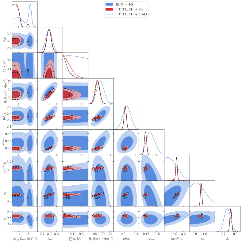
Figure 1: Marginalized constraints, at $68\%$ and $95\%$ confidence levels (CL), on the cosmological parameter of the self-interacting neutrino scenario when considering different combination of data.

IV Results and discussion

Whenever appropriate, we compare the results from the analysis of the self-interacting neutrino cosmologies with the results from the analysis of the $\Lambda$CDM model, for which we assume $\sum m_{\nu}=0.06\>\mathrm{eV}$. To distinguish the effects produced by delaying the neutrino free streaming from the effects induced by $N_{\mathrm{eff}}$ and $\sum m_{\nu}$, we additionally analyze an extension of the standard cosmological model, where the effective number of relativistic species, $N_{\mathrm{eff}}$, and the sum of neutrino masses, $\sum m_{\nu}$, are considered as free parameters. We dubbed this extension as $\Lambda$CDM + $N_{\mathrm{eff}}$ + $\sum m_{\nu}$. We use GetDist [131] to obtain most of the figures and tables displayed in this section.

IV.1 Bayesian analysis

IV.1.1 Cosmological constraints

Using the NS algorithm (see Section III.2), we derive constraints on the neutrino self-interaction, $\Lambda$CDM, and $\Lambda$CDM + $N_{\mathrm{eff}}$ + $\sum m_{\nu}$ models considering the combination of $\mathrm{TT,EE,TE}\>+\>\mathrm{FS}$ and $\mathrm{TT,EE,TE}\>+\>\mathrm{BAO}$ data. Although analyses neglecting Planck polarization data can be used to evaluate how the statistical significance of the strongly self-interacting neutrino scenario varies in the light of this data, we have found that analyses of this kind yield to unstable posterior inference, see Appendix A. Yet, we evaluate the role that Planck polarization power spectrum observations play in the statistical significance of the SI_ν scenario employing the profile likelihood approximation, see Sec. IV.2. For completeness, we recall the constraints obtained in our previous CMB-independent analysis [62], which uses FS data and Big Bang Nucleosynthesis priors on the primordial abundance of helium and deuterium coming from Ref. [132] and Ref. [133], respectively. We label this result as $\mathrm{BBN\>+\>FS}$. Our results are shown in Figs. 1, 2 and 3 and Tables 2 and 3.

Figure 1 shows the constraints on the self-interacting neutrino scenario for the different combinations of data considered in this section. We observe that $\mathrm{TT,EE,TE}\>+\>\mathrm{FS}$ (red contours and lines) and $\mathrm{TT,EE,TE}\>+\>\mathrm{BAO}$ (dashed black contours and lines) data yield similar constraints for most cosmological parameters (see also Tables 2 and 3). However, two notable differences arise. First, we note a moderately stronger constraint on $\sum m_{\nu}$ in the presence of BAO data. This moderate decrease in $\sum m_{\nu}$ uncertainty denotes that current geometrical measurements of the BAO can more effectively constrain the expansion history of the Universe and, consequently, the existence of non-relativistic species today. Furthermore, similar but weaker variations can be observed in $N_{\mathrm{eff}}$ and $H_{0}$ uncertainties.

Second, and more significantly, comparing both analyses reveals a notable reduction in the peak height of the SI_ν mode when analyzing the galaxy power spectrum data. While our cross-check analysis provided by the heuristic MH pooling method partially attributes such a decrease to NS deficiencies in exploring the intricate parameter space featured by the combination of CMB and LSS data, see Sec. III.3, we emphasize that this reduction indicates a depreciation in the statistical significance of the delayed neutrino free streaming scenario.

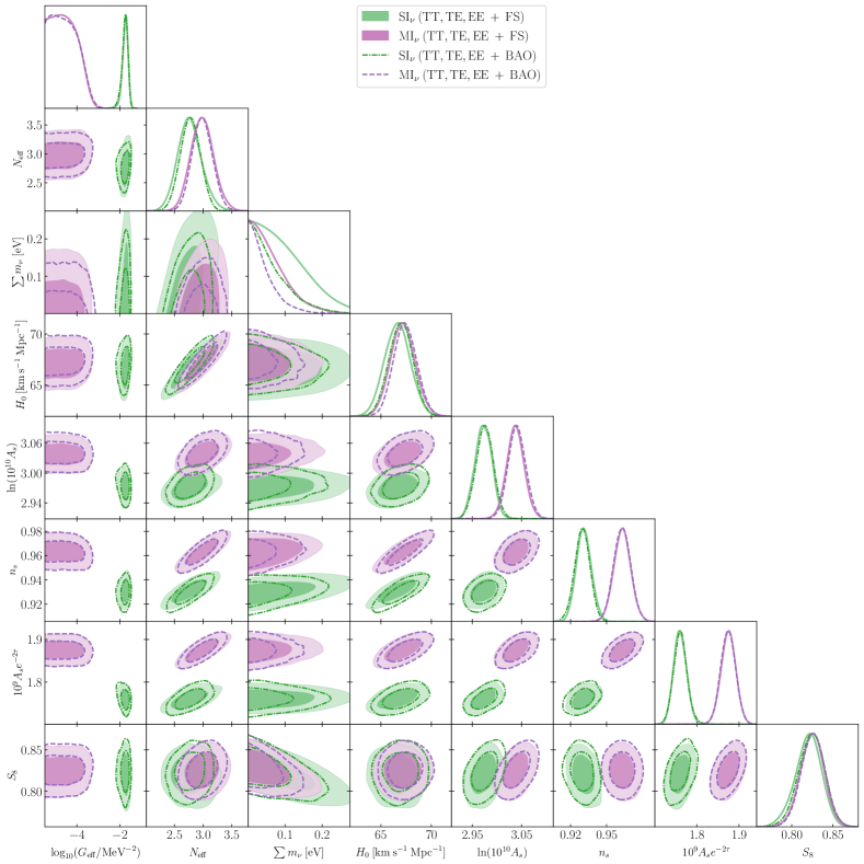
Figure 2: Comparison between the marginalized constraints, at $68\%$ and $95\%$ CL, on the cosmological parameter of the SI_ν and MI_ν modes when considering $\mathrm{TT,EE,TE}\>+\>\mathrm{FS}$ and $\mathrm{TT,EE,TE}\>+\>\mathrm{BAO}$ data.

Figure 1 additionally reveals that the challenge of simultaneously fitting the CMB and galaxy power spectra employing the simplest neutrino self-interaction scenario relates to a mild discrepancy in $\ln(10^{10}A_{\rm s})$ between the CMB and LSS data. By comparing the constraints obtained from $\mathrm{TT,EE,TE}\>+\>\mathrm{FS}$ (red contours and lines) and $\mathrm{BBN}\>+\>\mathrm{FS}$ (blue contours and lines), we note that the considerably smaller values of $\ln(10^{10}A_{\rm s})$ preferred by the CMB-independent analysis are disfavored by the inclusion of CMB data at $\gtrsim 2\sigma$. Although this intermediate discrepancy, associated with the $S_{8}$ tension [see Ref.  134, and references therein], is also present in the standard cosmological model, it primarily affects the SI_ν mode.

As discussed in Sec. II, a delay in the onset of neutrino free streaming induces a scale-dependent alteration of the linear power spectrum, including a suppression of its amplitude at scales crossing the horizon when neutrino are tight-coupled. Ref. [62] shows that, in light of the galaxy power spectrum data, the SI_ν mode compensates for such a change by modifying the primordial curvature power spectrum, characterized by the parameters $A_{\rm s}$ and $n_{\rm s}$. Although the CMB data allows for a similar modification, the mild $A_{\rm s}$ discrepancy restrains the latter to be more conservative, spoiling then the fit to the galaxy power spectrum data and the statistical significance of a cosmological scenario with strongly self-interacting neutrinos, see also Sec. IV.2.

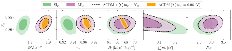
Figure 3: 2d marginalized constraints, at $68\%$ and $95\%$ CL, on the $\Lambda$CDM, $\Lambda$CDM + $N_{\mathrm{eff}}$ + $\sum m_{\nu}$, SI_ν, and MI_ν models obtained when analyzing $\mathrm{TT,EE,TE}\>+\>\mathrm{FS}$ data.

Table 2: 68$\%$ CL intervals for the cosmological parameters obtained from the analysis of the $\mathrm{TT,EE,TE}\>+\>\mathrm{FS}$ data for the different cosmologies here considered.

TT, TE, EE + FS
Parameter	$\Lambda$CDM	$\Lambda$CDM + $N_{\mathrm{eff}}$ + $\sum m_{\nu}$	MIν	SIν
$\log_{10}(G_{\mathrm{eff}}/\mathrm{MeV}^{-2})$	…	…	$<-4.25$	$-1.74^{+0.14}_{-0.11}$
$N_{\mathrm{eff}}$	$...$	$2.97\pm 0.20$	$2.99\pm 0.20$	$2.77^{+0.19}_{-0.22}$
$\sum m_{\nu}\,[\mathrm{eV}]$	$...$	$<0.08$	$<0.08$	$<0.12$
$10^{2}\omega_{\mathrm{b}}$	$2.239\pm 0.013$	$2.234\pm 0.018$	$2.234\pm 0.018$	$2.238^{+0.018}_{-0.020}$
$\omega_{\mathrm{cdm}}$	$0.1196\pm 0.001$	$0.1185\pm 0.0033$	$0.1187\pm 0.0032$	$0.1165^{+0.0032}_{-0.0037}$
$H_{0}\,[\mathrm{km\>s}^{-1}\>\mathrm{Mpc}^{-1}]$	$67.53\pm 0.44$	$67.1\pm 1.2$	$67.2\pm 1.2$	$66.6\pm 1.3$
$\ln(10^{10}A_{\rm s})$	$3.041\pm 0.016$	$3.038\pm 0.018$	$3.037\pm 0.018$	$2.973\pm 0.017$
$n_{\rm s}$	$0.9660\pm 0.004$	$0.9639\pm 0.007$	$0.9631\pm 0.007$	$0.9311\pm 0.006$
$\tau_{\mathrm{reio}}$	$0.054\pm 0.008$	$0.053\pm 0.008$	$0.053\pm 0.008$	$0.052\pm 0.007$
$\sigma_{8}$	$0.8086\pm 0.007$	$0.805^{+0.016}_{-0.013}$	$0.806^{+0.016}_{-0.013}$	$0.800^{+0.020}_{-0.014}$
$S_{8}$	$0.826\pm 0.012$	$0.824\pm 0.015$	$0.825\pm 0.014$	$0.820^{+0.017}_{-0.014}$
$10^{9}A_{\rm s}e^{-2\tau}$	$1.881\pm 0.011$	$1.876\pm 0.018$	$1.875\pm 0.017$	$1.761\pm 0.015$

Table 3: 68$\%$ CL intervals for the cosmological parameters obtained from the analysis of the $\mathrm{TT,EE,TE}\>+\>\mathrm{BAO}$ data for the different cosmologies here considered.

TT, TE, EE + BAO
Parameter	$\Lambda$CDM	$\Lambda$CDM + $N_{\mathrm{eff}}$ + $\sum m_{\nu}$	MIν	SIν
$\log_{10}(G_{\mathrm{eff}}/\mathrm{MeV}^{-2})$	…	…	$<-4.25$	$-1.77^{+0.16}_{-0.10}$
$N_{\mathrm{eff}}$	$...$	$2.97\pm 0.18$	$2.99\pm 0.18$	$2.78\pm 0.17$
$\sum m_{\nu}\,[\mathrm{eV}]$	$<0.051$	$<0.051$	$<0.05$	$<0.08$
$10^{2}\omega_{\mathrm{b}}$	$2.240\pm 0.014$	$2.234\pm 0.019$	$2.234\pm 0.018$	$2.236\pm 0.019$
$\omega_{\mathrm{cdm}}$	$0.1193\pm 0.001$	$0.1183\pm 0.003$	$0.1185\pm 0.003$	$0.1165\pm 0.0031$
$H_{0}\,[\mathrm{km\>s}^{-1}\>\mathrm{Mpc}^{-1}]$	$67.65\pm 0.46$	$67.3\pm 1.1$	$67.4\pm 1.1$	$67.0\pm 1.2$
$\ln(10^{10}A_{\rm s})$	$3.045\pm 0.016$	$3.041\pm 0.018$	$3.041\pm 0.018$	$2.975\pm 0.017$
$n_{\rm s}$	$0.9664\pm 0.004$	$0.9637\pm 0.007$	$0.9630\pm 0.007$	$0.9298\pm 0.006$
$\tau_{\mathrm{reio}}$	$0.056\pm 0.008$	$0.055\pm 0.008$	$0.055\pm 0.008$	$0.053\pm 0.007$
$\sigma_{8}$	$0.809\pm 0.007$	$0.810^{+0.015}_{-0.012}$	$0.811^{+0.014}_{-0.013}$	$0.809^{+0.017}_{-0.014}$
$S_{8}$	$0.824\pm 0.013$	$0.825\pm 0.015$	$0.826\pm 0.014$	$0.824^{+0.016}_{-0.015}$
$10^{9}A_{\rm s}e^{-2\tau}$	$1.881\pm 0.011$	$1.875\pm 0.018$	$1.874\pm 0.017$	$1.761\pm 0.016$

We display in Fig. 2, the corresponding constraints on the SI_ν (green contours and lines) and MI_ν (lilac contours and lines) modes obtained from the analyses of $\mathrm{TT,EE,TE}\>+\>\mathrm{FS}$ (solid contours and lines) and $\mathrm{TT,EE,TE}\>+\>\mathrm{BAO}$ (dashed contours and lines) data. The separation of the modes was obtained using the Hierarchical Density-Based Spatial Clustering of Applications with Noise (HDBSCAN) algorithm [135, 136, 137]. In agreement with the discussion presented above, it is noted that both analyses leads to similar constraints on most cosmological parameters, with modest differences in $\sum m_{\nu}$, $N_{\mathrm{eff}}$, and $H_{0}$. This indicates that, due to its higher accuracy, CMB data dominate the cosmological constraints.

As mentioned before, in light of the galaxy and CMB power spectra, the changes induced in the evolution of the cosmological perturbations by a strongly self-interacting neutrino scenario are reabsorbed by a modification of the primordial curvature power spectrum, specifically by a decrease on the values of its amplitude, $A_{\rm s}$, and tilt, $n_{\rm s}$. Such decreases are explicitly illustrated in Fig. 2 by the differences between the green and lilac constraints on $A_{\rm s}$ and $n_{\rm s}$ parameters. The difference between a strongly self-interacting neutrino scenario and its mildly counterpart, pragmatically reassembling the standard paradigm, is even more noticeable when comparing the constraints obtained for the amplitude of the CMB temperature spectrum, $A_{\rm s}e^{-2\tau}$.

Figure 3 offers a explicit comparison among SI_ν (green contours), MI_ν (lilac contours), $\Lambda$CDM (orange contours), and $\Lambda$CDM + $N_{\mathrm{eff}}$ + $\sum m_{\nu}$ (dashed black contours) models when considering the $\mathrm{TT,EE,TE}\>+\>\mathrm{FS}$ combination of data. Given that current cosmological data is insensitive to models with $\log_{10}(G_{\mathrm{eff}}/\mathrm{MeV}^{-2})\lesssim-4.5$, we observe that constraints for the MI_ν mode and $\Lambda$CDM + $N_{\mathrm{eff}}$ + $\sum m_{\nu}$ model are indistinguishable. In agreement to this, constraints obtained for the mildly self-interacting neutrinos concur with the $\Lambda$CDM constraints. Conversely, constraints on the strongly self-interacting neutrino cosmology highly deviate from the standard scenario, specially for the $A_{\rm s}e^{-2\tau}$ and $n_{\rm s}$ parameters. Similar features can be observed in Tables 2 and 3, which show the constraints for the aforementioned models for the analyses considering $\mathrm{TT,EE,TE}\>+\>\mathrm{FS}$ and $\mathrm{TT,EE,TE}\>+\>\mathrm{BAO}$ data, respectively.

We assessed the robustness of the HDBSCAN algorithm in accurately separating modes by repeating the clustering analysis using an alternative approach. In such an approach, we first identified the value of $\log_{10}(G_{\mathrm{eff}}/\mathrm{MeV}^{-2})$ that yields the lowest value of its corresponding one-dimensional marginalized posterior. This value is then employed to partition the NS chains into two regions corresponding to the SI_ν and MI_ν modes. We found that this alternative method and the HDBSCAN algorithm produce identical results.

IV.1.2 Model comparison

The Bayes evidence serves as a metric for assessing the efficacy of a model in light of a specific data set. For a given model, $\mathcal{M}$, the Bayesian evidence, or marginalized likelihood, is computed as follows:

$$\mathcal{Z}\equiv p(d|\mathcal{M})=\int\mathcal{L}(d|\theta,\mathcal{M})\pi(\theta|\mathcal{M})\>\mathrm{d}\theta\,,$$ (5)

where $\mathcal{L}(d|\theta,\mathcal{M})$ represents the likelihood, $\pi(\theta|\mathcal{M})$ denotes the priors, $d$ is the provided data and $\theta$ is the set of model’s parameters. Relying on the Bayesian evidence, a model comparison analysis can be performed by using the the Bayes factor, $\mathcal{B}_{ij}$, which contrasts the performance of two models through [138]:

$$\mathcal{B}_{ij}=\frac{p(d|\mathcal{M}_{i})}{p(d|\mathcal{M}_{j})}\,.$$ (6)

A value $\mathcal{B}_{ij}>1$ indicates that data increasingly prefer model $\mathcal{M}_{i}$ over model $\mathcal{M}_{j}$. If $\mathcal{B}_{ij}<1$, the opposite is inferred.

Table 4: Results of the model comparison analysis when $\mathrm{TT,EE,TE}\>+\>\mathrm{FS}$ data is considered and the standard paradigm is used as reference model, i.e., $\mathcal{M}_{0}=\Lambda$CDM. We emphasize that $\Delta\chi^{2}\equiv\Delta\chi^{2}_{\mathrm{model}}-\Delta\chi^{2}_{\Lambda\mathrm{CDM}}$. Values shown in parenthesis correspond to results obtained when analyzing the $\mathrm{TT,EE,TE}\>+\>\mathrm{BAO}$ combination of data.

Data	$\Lambda$CDM + $N_{\mathrm{eff}}$ + $\sum m_{\nu}$	MIν	SIν
$\Delta\chi^{2}_{\mathrm{FS}}$	$-0.08$	$-0.38$	$0.20$
$\Delta\chi^{2}_{\mathrm{high}\>\ell}$	$-0.77$	$-0.39$	$-0.78$
$\Delta\chi^{2}_{\mathrm{low}\>\ell}$	$-0.53$	$-0.41$	$3.05$
$\Delta\chi^{2}_{\mathrm{total}}$	$-1.38$	$-1.19$	$2.46$
$\Delta\mathrm{AIC}_{i0}$	$2.62$	$4.81$	$8.46$
$B_{i0}$	$0.031\pm 0.0062$ ($0.025\pm 0.0041$)	$0.106\pm 0.022$ ($0.053\pm 0.0089$)	$0.0007\pm 0.0005$ ($0.0027\pm 0.0008$)

Table 5: Results of the model comparison when analyzing $\mathrm{TT,EE,TE}\>+\>\mathrm{FS}$ data. We denote the reference model by $\mathcal{M}_{0}$ and define $\Delta\chi^{2}\equiv\Delta\chi^{2}_{\mathrm{model}}-\Delta\chi^{2}_{\mathcal{M}_{0}}$.

Data	$\mathcal{M}_{0}=\Lambda$CDM + $N_{\mathrm{eff}}$ + $\sum m_{\nu}$	$\mathcal{M}_{0}=$ MIν
$\Delta\chi^{2}_{\mathrm{total}}$	$3.84$	$3.65$
$\Delta\mathrm{AIC}_{i0}$	$5.84$	$3.65$
$B_{i0}$	$0.023\pm 0.015$	$0.0066\pm 0.0045$

It is worth mentioning that the Bayes factor compares the marginalized likelihood of two distinct models, $p(d|\mathcal{M})$, rather than the posterior probability of the models, $p(\mathcal{M}|d)$. While one could argue for a direct model comparison by evaluating the posterior odds:

$$\frac{p(\mathcal{M}_{i}|d)}{p(\mathcal{M}_{j}|d)}=\mathcal{B}_{ij}\frac{p(\mathcal{M}_{i})}{p(\mathcal{M}_{j})}\,,$$ (7)

we note that, overall, in agnostics analyses, there is no a priori reason to assume $p(\mathcal{M}_{i})/p(\mathcal{M}_{j})\neq 1$.

Complementary to the Bayes factor, whose values are computed using the NS algorithm, see Sec. III.2, we also consider the Akaike information criterion (AIC) [139]:

$$\mathrm{AIC}=\chi^{2}_{\mathrm{min}}+2n\,,$$ (8)

where $n$ is the number of parameters to fit, and $\chi^{2}_{\mathrm{min}}$ is the minimum chi-square fit to the data. The quality of fit between distinct models can then be evaluated by:

$$\Delta\mathrm{AIC}_{ij}\equiv\mathrm{AIC}_{i}-\mathrm{AIC}_{j}=\Delta\chi^{2}_{ij}+2\Delta n\,,$$ (9)

with $\Delta n$ being the difference in the number of parameters between $\mathcal{M}_{i}$ and $\mathcal{M}_{j}$ models. The AIC criterion favors the model with the lower value; thus, a positive (negative) $\Delta\mathrm{AIC}_{ij}$ indicates a preference for model $\mathrm{M}_{j}$ ($\mathrm{M}_{i}$).

Unless otherwise stated, we use the $\Lambda$CDM model as the reference model, i.e., we compute $\mathcal{B}_{i0}$ and $\Delta\mathrm{AIC}_{i0}$ considering $\mathcal{M}_{0}=\Lambda$CDM. Table 4 displays the values of $\Delta\mathrm{AIC}_{i0}$ and $\mathcal{B}_{i0}$ obtained from the analysis of $\mathrm{TT,EE,TE}\>+\>\mathrm{FS}$ data. For completeness, we individually list the minimum chi-square fit both for the different likelihoods used in the analyses and the total combination of them. We additionally display the Bayes factor corresponding to the analysis of $\mathrm{TT,EE,TE}\>+\>\mathrm{BAO}$ data. Results of this extra analysis are shown in parentheses in the last row of Table 4.

As expected, both the $\Lambda$CDM + $N_{\mathrm{eff}}$ + $\sum m_{\nu}$ model and MI_ν mode yield comparable values of $\Delta\chi^{2}_{\mathrm{total}}<0$, denoting that both cosmologies offer a better fit to the data than the standard paradigm. However, as indicated by the values of the $\Delta\mathrm{AIC}_{i0}$ and $\mathcal{B}_{i0}$ estimators, this enhancement in the goodness of fit is insufficient to compensate for the inclusion of the neutrino parameters.

A comparison between the values of $\mathcal{B}_{i0}$ and $\Delta\chi^{2}_{\mathrm{total}}$ obtained for the $\Lambda$CDM + $N_{\mathrm{eff}}$ + $\sum m_{\nu}$ model reveals that the preference for the standard paradigm, over the $\Lambda$CDM extension, is primarily due to Occam’s razor principle — the data suggest that introducing the $N_{\mathrm{eff}}$ and $\sum m_{\nu}$ parameters does not yield significant statistical improvements. In practice, this is related to the current inability of cosmological data to detect the mass of neutrinos; see Fig. 3 and Table 2, for instance. In addition, according to the Bayes factor, data slightly favors the MI_ν mode over the $\Lambda$CDM + $N_{\mathrm{eff}}$ + $\sum m_{\nu}$ model with odds of approximately $3:1$. Although this slight preference lacks statistical significance, the subtle inclination towards a scenario where the free-streaming phenomenology of neutrinos is constrained by the data could hint that cosmological data response better to $\log_{10}(G_{\mathrm{eff}}/\mathrm{MeV}^{-2})$ rather than $\sum m_{\nu}$. One could speculate that data could prefer cosmological scenarios with more complex neutrino physics rather than the simple phenomenological approach presented by $\Lambda$CDM + $N_{\mathrm{eff}}$ + $\sum m_{\nu}$.

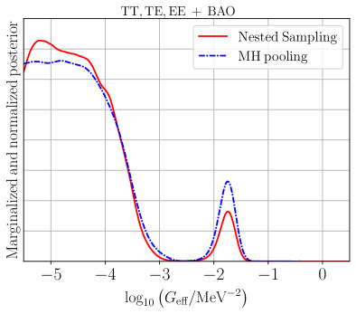
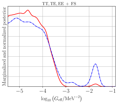
Figure 4: 1d marginalized (and normalized) $\log_{10}(G_{\mathrm{eff}}/\mathrm{MeV}^{-2})$ posterior obtained when analyzing $\mathrm{TT,EE,TE}\>+\>\mathrm{FS}$ (right) and $\mathrm{TT,EE,TE}\>+\>\mathrm{BAO}$ (left) data employing the MH pooling (dashed blue lines) and NS (red solid lines) techniques.

Regarding the SI_ν mode, we observe a deterioration in the goodness of the fit, yielding $\Delta\chi^{2}_{\mathrm{total}}\approx 2.5$. Such degradation is primarily attributed to a worsening of the fit in the CMB low $\ell$ power spectra data, which features $\Delta\chi^{2}_{\mathrm{low\>\ell}}=3.05$. Furthermore, the combination of CMB and galaxy data displays $\Delta\chi^{2}_{\mathrm{FS}}=0.2$, indicating that when CMB observations are considered in the analysis, the SI_ν mode provides a worse fit to the galaxy power spectrum compared to the $\Lambda$CDM model. It is interesting to highlight that this stands contrary to the CMB-independent analysis, where the strongly self-interacting neutrino cosmology fits the LSS data better than the standard paradigm with $\Delta\chi^{2}\approx-2.5$ [62]. As discussed before, the worsening of SI_ν galaxy power spectrum fit relates to the mild discrepancy in $\ln(10^{10}A_{\rm s})$ owing to the fact CMB data excludes significantly lower values of $A_{\rm s}$.

The preference displayed by the combination of $\mathrm{TT,EE,TE}\>+\>\mathrm{FS}$ data for the $\Lambda$CDM model over the SI_ν scenario is further noted in $\Delta\mathrm{AIC}_{i0}\sim 8.5$ and, remarkably, the Bayes factor, which indicates that the strongly self-interacting neutrino cosmology is disfavoured with odds of $7:10000$. While this significant lower value calls attention to the difficulty of fitting the data with the simplest representation of delayed neutrino free streaming scenario, we note that the small support for the SI_ν mode is not merely induced by the self-interactions, i.e., $\log_{10}(G_{\mathrm{eff}}/\mathrm{MeV}^{-2})$. As shown by Table 5, more conservative values of the Bayes factor are obtained when the SI_ν mode is compared to the $\Lambda$CDM + $N_{\mathrm{eff}}$ + $\sum m_{\nu}$ and MI_ν models, indicating that $\sum m_{\nu}$ plays an important role in the limited support found for strongly self-interacting neutrinos. However, all the analyses suggest that the SI_ν scenario encounters several challenges in providing a self-consistent interpretation of the observed CMB and galaxy power spectra.

Compared to the analysis of $\mathrm{TT,EE,TE}\>+\>\mathrm{BAO}$ data, whose results are shown in parentheses in the last row of Table 4, analysis considering $\mathrm{TT,EE,TE}\>+\>\mathrm{FS}$ provides similar results for all models except for the SI_ν scenario. Indeed, a reduction of factor $\sim 4$ in the Bayes factor is observed when galaxy power spectrum data is considered instead of the geometrical distance provided by BAO measurements. Furthermore, we notice that, in the analyses considering the galaxy power spectrum data, values found of the Bayes factor regarding the SI_ν mode feature substantial uncertainties. This issue is discussed below.

IV.1.3 Cross-checking NS results

The combination of $\mathrm{TT,EE,TE}\>+\>\mathrm{FS}$ and $\mathrm{TT,EE,TE}\>+\>\mathrm{BAO}$ data is additionally analyzed using the heuristic method outlined in Sec. III.3. The marginalized $\log_{10}(G_{\mathrm{eff}}/\mathrm{MeV}^{-2})$ posterior distributions obtained from both this method and the NS algorithm are presented in in Fig. 9.

We observe that, for both combinations of data, the marginalized posteriors provided by the MH pooling method (dashed blue lines) show higher SI_ν peaks than the NS posteriors (solid red line). In the case of the analysis considering BAO data (left panel), we note a slight difference between the MH pooling and NS method. This mismatch can be attributed to the intrinsic sampling error induced by both methods in the final kernel density estimation of the posterior. Conversely, the notable difference observed in the case of the analysis of CMB and galaxy power spectra (right panel) data could hint to a deficient NS exploration that fails to accurately portray the relative height between the MI_ν and SI_ν modes. It is noteworthy to mention that a comparison of the goodness of fit of the MI_ν and SI_ν modes yields $\Delta\chi^{2}_{\mathrm{total}}=3.65$ (see Table 5) implying a maximum likelihood ratio of $[\mathcal{L}^{\mathrm{MI}_{\nu}}/\mathcal{L}^{\mathrm{SI}_{\nu}}]_{\mathrm{max}}\sim 6$. Right panel of Fig. 9 shows that the NS algorithm (solid red line) overestimates this ratio.

An examination of the final NS product reveals a sampling bias favoring the MI$\nu$ mode. Specifically, we found that our NS exploration produces few samples for the SI$\nu$ mode within the $68\%$ confidence level. While pinpointing the precise cause of this bias is beyond the scope of this paper, it likely relates to the specific resolution assumed in our analyses, i.e., the number of NS live points. In this context, it is important to highlight that the likelihoods used here encompass a complex parameter space, expanding from ten to twenty-two dimensions when considering FS data instead of BAO measurements in the analysis. Thus, while one could theoretically increase the NS resolution, in practice, the complexity of the parameter space suggests that overcoming this bias might be challenging without significantly increasing computational time.

The sampling bias is also noticeable in the uncertainties of the evidence of the SI_ν mode when $\mathrm{TT,EE,TE}\>+\>\mathrm{FS}$ data is analyzed. Employing this data, NS algorithm provides a $15\%$ estimation of evidence for the MI_ν mode while a $70\%$ estimation for the SI_ν mode. As indicated by Table 5 and the last column of Table 4, these uncertainties play a dominant role in the errors associated with the Bayes factor, $\mathcal{B}_{i0}$, whose values are attained with approximately $70\%$ accuracy for the strongly self-interacting neutrino scenario. While significant, it is crucial to highlight that, at first approximation, these errors would enlarge (reduce) the value obtained for $\mathcal{B}_{i0}$ by a factor of $\sim 2$ ($\sim 0.5$), marginally affecting the level of support that data display for the simplest representation of delayed neutrino free streaming cosmology.

We argue that the challenges encountered in exploring the parameter space are related to the complexity of modeling the state-of-the-art cosmological data. Acknowledging that upcoming observations are unlikely to be less complex to model within a Bayesian likelihood-based framework, we emphasize the importance of recognizing and assessing the potential limitations of the diverse statistical methods employed in cosmological inference. Even when the challenges encountered in exploring the parameter space in this study may not be directly applicable to other analyses, discarding potential deficiencies will be fundamental in exploring new physics, particularly when analyzing nonstandard scenarios that, despite deviating significantly from the standard paradigm, can provide a good fit for cosmological observables.

Lastly, it is important to stress that the heuristic method employed could also fail to accurately estimate the real posterior. The MH pooling method not only inherits the potential deficiencies of the typical MH algorithm but could also suffer from errors induced in the re-weighting process (see Appendix B for further discussion). We argue, however, that this method serves as a first approximation to expose potential deficiencies on a NS exploration.

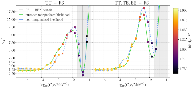
Figure 5: Profile likelihood of the $\log_{10}(G_{\mathrm{eff}}/\mathrm{MeV}^{-2})$ parameter obtained from the analyses of $\mathrm{TT,EE,TE}\>+\>\mathrm{FS}$ (right) and $\mathrm{TT}\>+\>\mathrm{FS}$ (left) data when considering the nuisance-marginalized (circles and solid green lines) and non-marginalized (cross marks and dashed light blue lines) versions of Planck likelihoods. The color scheme of the circles and cross marks indicates the best-fit value of $10^{9}A_{\rm s}e^{-2\tau}$ at the respective $\log_{10}(G_{\mathrm{eff}}/\mathrm{MeV}^{-2})$. The horizontal solid gray lines and bands denote the $\log_{10}(G_{\mathrm{eff}}/\mathrm{MeV}^{-2})$ best-fit and $68\%$ CL interval obtained from the CMB-independent analysis [62], respectively.

IV.2 Volume effects

We profile the $\log_{10}(G_{\mathrm{eff}}/\mathrm{MeV}^{-2})$ likelihood considering both the $\mathrm{TT}\>+\>\mathrm{FS}$ and $\mathrm{TT,EE,TE}\>+\>\mathrm{FS}$ data combination. To assess possible volume effects resulting from the marginalization of the CMB foreground and nuisance parameters, we perform the analysis employing both the nuisance-marginalized and non-marginalized versions of the CMB likelihoods, see Sec. III. Results of our analyses are shown in Fig. 5. We quantify the goodness of fit of the self-interacting neutrino scenario relative to the $\Lambda$CDM model using $\Delta\chi^{2}=\chi^{2}_{\mathrm{model}}-\chi^{2}_{\Lambda\mathrm{CDM}}$.

First, we observe that analyses employing either the nuisance-marginalized (solid green lines) or non-marginalized (dashed blue lines) versions of the Planck likelihoods yield comparable results. This similarity suggests that astrophysical foregrounds and instrumental modeling parameters are unlikely to exhibit significant degeneracy with the effects produced by neutrino interactions. Consequently, assumptions made to provide a more compact CMB-only Planck likelihood [140] are expected to hold for a delayed neutrino free streaming scenario.

Second, in agreement with earlier studies [see 28, for instance], we note that the SI_ν mode offers a competitive fit to the combination of the CMB temperature and galaxy power spectra. As shown by the left panel of Fig. 5, the best-fit value obtained when analyzing $\mathrm{TT}\>+\>\mathrm{FS}$ data not only yields $\Delta\chi^{2}\approx-2.5$ but also agrees very well with the results of our previous CMB-independent analysis; in both cases the best-fit value features $\log_{10}(G_{\mathrm{eff}}/\mathrm{MeV}^{-2})\approx-1.3$. However, as displayed in the right panel, the statistical significance of the SI_ν mode is overshadowed by the Planck polarization data, resulting in $\Delta\chi^{2}\approx 2.5$.

The fact that a strongly self-interacting neutrino scenario can provide a good fit to galaxy and CMB temperature power spectra data but fails to explain the Planck polarization observations can be understood by examining how cosmological data constrain the amplitude of the CMB power spectrum, denoted by $10^{9}A_{\rm s}e^{-2\tau}$. In the absence of polarization data, the parameters $A_{\rm s}$ and $\tau_{\mathrm{reio}}$ are strongly degenerate, implying that temperature data can merely constrain the combination $10^{9}A_{\rm s}e^{-2\tau}$ but not $A_{\rm s}$ and $\tau_{\mathrm{reio}}$ independently. Thus, the CMB temperature power spectrum allows the $A_{s}$ values that the SI_ν scenario requires to fit the galaxy power spectrum significantly. However, the polarization power spectrum, sensitive to the reionization, can break down this degeneracy, imposing important constraints on $\tau_{\mathrm{reio}}$ and $A_{\rm s}$. Such constraints exclude the lower values of $A_{\rm s}$ needed to compensate for the effect of delaying the neutrino free streaming, diminishing the statistical significance of the strongly self-interacting neutrino cosmology.

The role of CMB polarization data in the analysis is further illustrated by the color scheme of the circle and cross marks in Fig. 5. From both panels we note that in the MI_ν regime, the best-fit values found for the CMB amplitude agree with the typical value expected in the standard paradigm, i.e., $10^{9}A_{\rm s}e^{-2\tau}\approx 1.88$ [see Ref. 1, for instance]. Conversely, as one transitions towards the SI_ν regime, lower values of $10^{9}A_{\rm s}e^{-2\tau}$ are obtained. While the temperature power spectrum allows such values (left panel), Planck polarization (right panel) can effectively constrain the reionization history, largely disfavouring scenarios with $10^{9}A_{\rm s}e^{-2\tau}\lesssim 1.85$ and thereby diminishing the goodness of fit of the SI_ν mode.

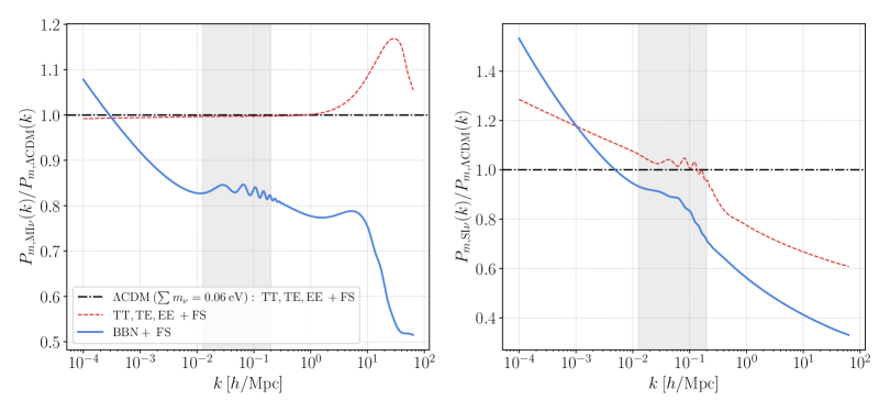
Figure 6: Ratio between the best-fit prediction for the linear power spectrum of the standard $\Lambda$CDM model and the MI_ν mode (left panel) or SI_ν mode (right panel) for the different combination of data considered. The gray band represents the range of scales probed by the galaxy power spectrum data.

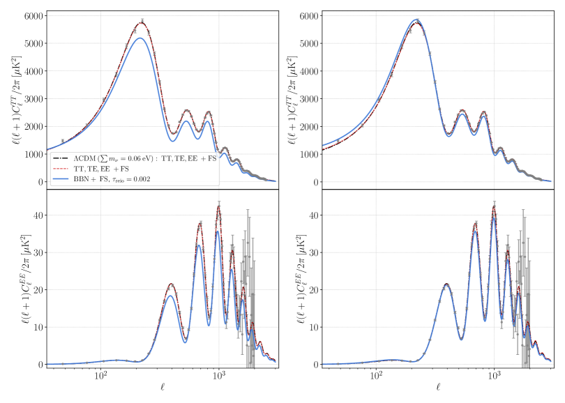
Figure 7: $\mathrm{TT}$ (top) and $\mathrm{EE}$ (bottom) CMB power spectra best-fit predictions for the $\Lambda$CDM (dot-dashed black lines), MI_ν (left panels), and SI_ν (right panels) cosmologies in light of different combination of data.

IV.3 Cosmological implications

Figures 6 and 7 illustrate the linear matter and CMB power spectra, respectively, predicted by the best-fit of the SI_ν (right panel) and MI_ν (left panel) modes for the analyses of $\mathrm{TT,EE,TE}\>+\>\mathrm{FS}$ (dashed red lines) and $\mathrm{BBN}\>+\>\mathrm{FS}$ (solid blue lines) data compared to the predictions provided by the $\Lambda$CDM best-fit (dot-dashed black lines) when analyzing the CMB and galaxy power spectra.

We first focus on the linear matter power spectrum. As shown by the dashed red line in the left panel of Fig. 6, in light of the same data, the $\Lambda$CDM model and MI_ν scenario provide comparable predictions across linear scales with a notable bump that peaks well inside nonlinear scales. On the other hand, a comparison between the baseline $\Lambda$CDM analysis with the best-fit of the MI_ν mode found in the CMB-independent analysis (solid blue line in the left panel) explicitly portrays the mild discrepancy in $A_{\rm s}$. We note that, even within the $\Lambda$CDM framework, analyses of the observed large-scale distribution of galaxies consistently yield lower values of the amplitude, $A_{\rm s}$, and tilt, $n_{\rm s}$, of the primordial curvature power spectrum compared to the CMB observations [see also Refs. 126, 119].

Contrary to this, the right panel of Fig. 6 shows that both in the absence (solid blue line) or presence (dashed red line) of CMB data, the SI_ν matter power spectrum exhibits a unchanging general structure: the strongly self-interacting neutrinos feature a barely visible bump that peaks around $k\sim 0.1\>h/\mathrm{Mpc}$ and predict an important suppression of structures on nonlinear scales. This distinct prediction is less pronounced when CMB power spectra are considered (dashed red line in the right panel), in which case the SI_ν best-fit predicts a $\gtrsim 20\%$ ($\gtrsim 30\%$) suppression of the power spectrum at galactic (sub-galactic) scales.

As discussed in Ref. [28], the suppression induced by a delay of the onset of neutrino free streaming can add to the step-like suppression featured by massive neutrinos [141, 142]. This characteristic points out a significant degeneracy between the free-streaming nature and the sum of masses of neutrinos, with potential implications for cosmological inference. One could imagine a scenario in which the Universe features a significant delay of the neutrino free streaming but cosmologists use a $\Lambda$CDM + $\sum m_{\nu}$ framework to analyze the data. In such a scenario, cosmological inference based on the large-scale galaxy distribution might overestimate the total mass of neutrinos, as the underlying analysis overlooks the true free-streaming nature of neutrinos. Hence, determining precisely whether our Universe follows the SM chronology will be crucial for enabling robust detection of the total mass of neutrinos using upcoming LSS data.

The mild discrepancy between the CMB and LSS data is also noted in Fig. 7, where we observe that the best-fit for the $\mathrm{BBN}\>+\>\mathrm{FS}$ (solid blue lines) data obtained within the SI_ν (right panels) and MI_ν (left panels) scenarios largely deviate from the $\Lambda$CDM analysis considering $\mathrm{TT,EE,TE}\>+\>\mathrm{FS}$ (dot-dashed black lines) data. Deviations between the baseline $\Lambda$CDM analysis and self-interacting neutrino models are less pronounced when simultaneously analyzing the CMB and galaxy power spectra (solid red lines).

V Conclusions

During the last decade, several analyses have shown that certain CMB data exhibit a non-trivial preference for a cosmological scenario in which the onset of neutrino free streaming is delayed until close to the epoch of matter-radiation equality. More recently, additional analyses have revealed that LSS data also support this scenario, dismissing the hypothesis of an accidental feature in the CMB data and intensifying the puzzle surrounding the free-streaming nature of neutrinos [62, 63]. Here, by adopting the simplest cosmological representation for self-interacting neutrinos, we investigated whether this nonstandard cosmology can provide a self-consistent scenario for both the CMB power spectra and the large-scale distribution of galaxies simultaneously. We conducted an exhaustive analysis of the parameter space using three different approaches: profile likelihood, nested sampling, and heuristic Metropolis-Hastings approximation. We robustly demonstrated that the observed large-scale distribution of galaxies exacerbates the challenge already posed by the CMB Planck polarization data for the strongly self-interacting neutrino cosmology. This indicates that the simplest representation of a Universe with delayed neutrino free streaming fails to accommodate a consistent cosmological picture for the both CMB and galaxy power spectra.

Our analysis points out that the difficulty of simultaneously fitting the CMB and galaxy power spectra employing the simplest neutrino self-interaction scenario relates to the $S_{8}$ tension. The mild discrepancy between the CMB power spectra and the large-scale distribution of galaxies, particularly in the amplitude of the primordial curvature power spectrum, $A_{\rm s}$, directly impacts the statistical significance of the strongly self-interacting neutrino cosmology, represented by the SI$\nu$ mode. The profile likelihood analysis reveals that Planck polarization data disfavor lower values of $A_{\rm s}$ required to compensate for the effects of neutrino interactions in the linear matter power spectrum. Based on the combination of CMB and galaxy power spectra data, our findings indicate that the SI_ν mode provides a mildly worse fit to the data when compared to the $\Lambda$CDM model, specifically, $\Delta\chi^{2}\approx 2.5$. This degradation is mainly due to a worsening of the fit of the CMB low $\ell$ power spectra data, which yield $\Delta\chi^{2}_{\mathrm{low\>\ell}}\approx 3.1$. Additionally, we observe that the SI_ν mode offers a worse fit to the galaxy power spectrum compared to the $\Lambda$CDM model, with a quantified difference of $\Delta\chi^{2}_{\mathrm{FS}}\approx 0.2$.

The challenge posed by the CMB and galaxy observations to the simple neutrino interaction model considered here is quantify through the Bayes factor. In particular, we have found that this nonstandard neutrino cosmology is disfavored over the standard paradigm with odds of $7:10000$. While this significantly lower value highlights the difficulty of providing a consistent cosmological picture for the data with a simple representation of delayed neutrino free streaming, we have noted that this is not solely induced by the presence of nonstandard interactions in the neutrino sector. Weaker results are found when accounting for the fact that current cosmological data cannot detect the sum of the masses of neutrinos, $\sum m_{\nu}$. In such cases, the analyses indicates that the data disfavor the SI_ν mode over the $\Lambda$CDM + $N_{\mathrm{eff}}$ + $\sum m_{\nu}$ and MI_ν cosmologies with odds of $23:1000$ and $66:10000$, respectively. The mild discrepancy in $A_{\rm s}$ and its impact on the SI_ν mode is further illustrated by the Bayes factor, whose value reduces by a factor of $\sim 4$ when the galaxy power spectrum data is considered instead of the BAO measurements.

It is crucial to highlight that although our analysis robustly reveals minor support (or no support at all) for the simplest representation of delayed free-streaming neutrino cosmology, it does not dismiss the SI_ν mode. Regardless of its microscopic origin, the enduring presence of the SI_ν mode in the CMB and galaxy power spectra data indicates that it is an actual physical feature present in the data. However, the fact that CMB and galaxy data significantly disfavor the simplest framework considered here emphasize the need for considering a broader range of phenomenologies [see Refs. 143, 60, 144, for instance]. Broadly, we argue that more realistic representation of the neutrino sector are needed to accommodate the cosmological data without conflicting with other laboratory constraints. Additionally, we bring attention to the fact the SI_ν signature observed in the data could also correspond to a yet-to-be-discovered phenomenon deep in the radiation-dominated epoch that is not related at all to the neutrino sector.

Although future analyses could help unveil the true nature of the SI_ν mode, we emphasize that significant challenges, for both the standard and nonstandard neutrino scenario, lie ahead. On the one hand, theoretical efforts will be needed to construct appropriate cosmological frameworks for more complex scenarios. In particular, new phenomenologies altering the evolution of the Universe at late times could affect the evolution of cosmological perturbations in the nonlinear regime, forcing us to reassess the way we model the LSS observables. On the other hand, given that the step-like suppression of the power spectrum produced by massive neutrinos adds to the effects of a delayed neutrino free streaming, analyses overlooking the underlying free-streaming nature of neutrinos could lead to biased estimations of the sum of the masses of neutrinos, $\sum m_{\nu}$. Understanding how our future analyses based on galaxy clustering data would change in light of this kind of effects will be then crucial to confirm the standard chronological evolution of the Universe or reveal the exact nature of the feature observed in the data.

Lastly, even when we adopt the simplest representation for a delayed free streaming scenario, our analysis of the state-of-the-art cosmology data proves computationally challenging. While our conclusions remain robust across distinct approaches, we have found that exploration of the parameter space of the simplest framework adopted here can suffer from significant inefficiencies at several levels. In particular, when relying on the generally advised nested sampling method, we observe biased posterior estimation when analyzing the CMB and galaxy power spectra. Although the same inefficiencies are not necessarily expected to emerge in more complex realizations of the SI_ν mode, we emphasize that identifying such inefficiencies is neither a trivial task nor always computationally feasible. Even when specific-oriented tools are available for this task [see 145, 113, 146, for instance], the complexity of modeling state-of-the-art cosmological data makes this problem inherently complex. Future observations are unlikely to ease this issue. Therefore, it is crucial to bear in mind the limitations of the statistical methods used in cosmological inference, especially when analyzing new physics that deviate from the typically proposed mild deformations of the $\Lambda$CDM model but can still provide a good fit to the cosmological observables.

Appendix A Additional runs with different nested sampling configuration

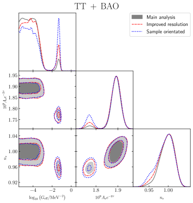
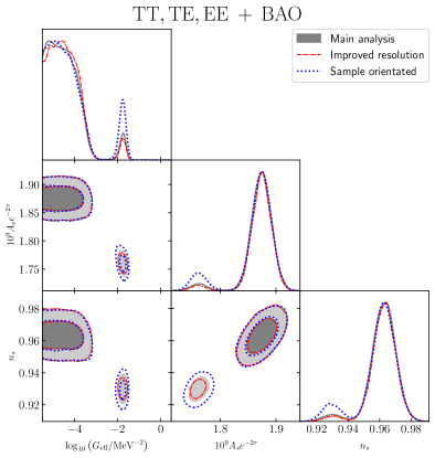
Figure 8: Comparison between the marginalized constraints, at $68\%$ and $95\%$ CL, on the relevant cosmological parameter of the self-interacting neutrino cosmology obtained when adopting three distinctive NS configurations and considering $\mathrm{TT}\>+\>\mathrm{BAO}$ (left plot) and $\mathrm{TT,EE,TE}\>+\>\mathrm{BAO}$ (right plot) data.

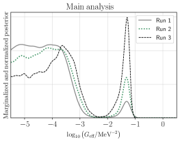
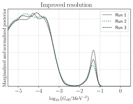
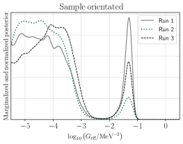
Figure 9: 1d marginalized (and normalized) $\log_{10}(G_{\mathrm{eff}}/\mathrm{MeV}^{-2})$ posterior obtained when analyzing $\mathrm{TT}\>+\>\mathrm{BAO}$ data adopting the main analysis (left panel), improved resolution (central panel), and sample oriented (right panel) NS configurations. We conduct the analysis for each configuration three different times.

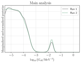
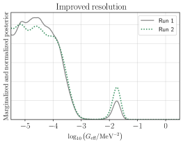
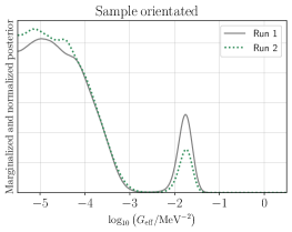
Figure 10: 1d marginalized (and normalized) $\log_{10}(G_{\mathrm{eff}}/\mathrm{MeV}^{-2})$ posterior obtained when analyzing $\mathrm{TT,TE,EE}\>+\>\mathrm{BAO}$ data adopting the main analysis (left panel), improved resolution (central panel), and sample oriented (right panel) NS configurations. We conduct the analysis for each configuration two different times.

Here, we present the results of additional analyses with varied NS configurations that could help to diagnose possible deficiencies in NS exploration. We consider the following configurations:

1. Main analysis configuration: $2000$ live points and a sampling efficiency of $0.3$,

2. Improved resolution configuration: same as previous configuration with improved resolution employing $3000$ live points,

3. Sample oriented configuration: $2000$ live points and a sampling efficiency of $0.75$.

In all these cases, we impose a minimum precision of $0.05$ in log-evidence. Due to the high-computational cost of analyzing the CMB and galaxy power spectra data, we only apply varied NS configuration to the combination of CMB and BAO data. We analyze $\mathrm{TT}\>+\>\mathrm{BAO}$ data performing three runs for each of the distinct configurations considered here. Furthermore, we perform two runs of each configuration when considering $\mathrm{TT,EE,TE}\>+\>\mathrm{BAO}$ data. Results are shown in Fig. 8, 9, and 10.

We find that the NS analysis disregarding Planck polarization data yields unstable constraints. Such constraints not only vary under different configurations of the NS framework, as shown by the left plot of Fig. 8, but also under different runs of the same setup, as seen in Fig. 9. We argue that this unstable behavior could be related to the intrinsic shape of the underlying posterior. As extensively discussed in the literature [105, 112, 113, 114, 115, 116], NS can exhibit limitations depending on the nature of the likelihood under scrutiny, particularly affected by likelihoods with plateaus. The simplest representation of the self-interacting neutrino model intrinsically features a likelihood plateau for mildly (weakly) coupling strength, as scenarios with $\log_{10}(G_{\mathrm{eff}}/\mathrm{MeV}^{-2})\lesssim-4$ are highly degenerate at (mildly) linear scale. Although this plateau is expected to impact the analysis independently of the combination of data considered, the absence of polarization data opens further degeneracies in the parameter space, complicating the problem. The CMB temperature power spectrum provides limited information about the reionization epoch, leading to loose constraints on the optical depth that are highly degenerate with the primordial amplitude $A_{s}$. This degeneration is reflected in the sum of the masses of neutrinos, whose parameter space widely opens up, allowing a large range of masses that modestly impact the value of the likelihood. The combination of the $\log_{10}(G_{\mathrm{eff}}/\mathrm{MeV}^{-2})$ plateau and loose constraints on $\sum m_{\nu}$ leads to the unstable nature found for the constraints coming from the analysis of $\mathrm{TT}\>+\>\mathrm{BAO}$ data.

Although more stable results are found when including the Planck polarization data in the analysis (see the right plot of Fig. 8), we note that constraints become slightly unstable when adopting a sample-oriented configuration (see the right panel of Fig. 10). Such slight instability could be related to the $\log_{10}(G_{\mathrm{eff}}/\mathrm{MeV}^{-2})$ plateau. Additionally, it is important to emphasize that even when the analysis of $\mathrm{TT,TE,EE}\>+\>\mathrm{BAO}$ seems to be mainly unaffected by the aforementioned plateau, the impact of this could be more noticeable in a more complex parameter space, for instance, the one featured by the $\mathrm{TT,TE,EE}\>+\>\mathrm{FS}$ data. Additionally, further complications unrelated to the underlying shape of the posterior could bias the NS exploration.

Appendix B Metropolis-Hasting pooling: proof of concept

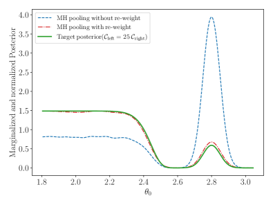
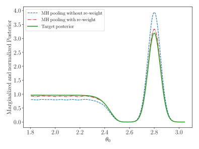
Figure 11: Results obtained from the MH pooling method, see Sec. III.3, when applied to two toys models mimicking, Eq. B, the $\log_{10}(G_{\mathrm{eff}}/\mathrm{MeV}^{-2})$ posterior.

As a proof of concept for the heuristic Metropolis-Hasting framework introduced in Sec. III.3, we analyze two toy models mimicking the expected $\log_{10}(G_{\mathrm{eff}}/\mathrm{MeV}^{-2})$ posterior. The toy models are built assuming a two-dimensional parameter space, $\hat{\theta}=\left\{\theta_{0},\theta_{1}\right\}$, with a marked bi-modality in $\theta_{0}$. Assuming $\theta_{0}$ and $\theta_{1}$ as uncorrelated variables, we model the bi-modality by imposing a likelihood encompassing a normal distribution and a generalized normal distribution that peak at different regions of the parameter space. More specifically, we adopt

$$\mathcal{L}(\theta_{0})= \mathcal{C}_{\mathrm{right}}\;\frac{1}{\sqrt{2\pi\sigma^{2}}}\exp{\left[-\frac{1}{2}\left(\frac{\theta_{0}-\mu_{1}}{\sigma}\right)^{2}\right]}$$

$$+ \frac{\mathcal{C}_{\mathrm{left}}}{2\alpha}\>\frac{\beta}{\Gamma(1/\beta)}\exp{\left[-\left(\frac{\theta_{0}-\mu_{2}}{\alpha}\right)^{\beta}\right]}\,,$$ (10)

where $\Gamma$ denotes the Gamma function, $\mu_{1}=2.8,\sigma=0.05,\mu_{2}=1.8,\alpha=0.65$, and $\beta=12$. The first term of this equation mimics the SI_ν mode, while the second term introduces a plateau-like behavior similar to the MI_ν mode. The ratio between $\mathcal{C}_{\mathrm{right}}$ and $\mathcal{C}_{\mathrm{left}}$ determines whether the plateau, expected at $\theta_{0}\rightarrow\mu_{2}$, dominates the posterior. We model two different scenarios assuming:

1. $\mathcal{C}_{\mathrm{left}}=25\>\mathcal{C}_{\mathrm{right}}$, emulating a posterior dominated by the plateau and saturating at $\mu_{2}$,

2. $\mathcal{C}_{\mathrm{left}}=3\>\mathcal{C}_{\mathrm{right}}$, emulating a posterior that peaks at $\mu_{1}$.

Considering a uniform prior $\theta_{0}=[1.8,3.0]$, we explore these models using the heuristic MH pooling method. Results of our analyses and the underlying real posterior are illustrated in Fig. 11.

We observe that, unlike a pooling approach where no re-weight is applied (dashed blue lines), our heuristic method (dot-dashed red lines) — following Eq. (3) to obtain the appropriate re-weighting factors — enables precise estimation of the target posterior (solid green lines). As shown by both panels of Fig. 11, the underlying posterior is recovered regardless of the relative height between the plateau at $\mu_{2}$ and peak at $\mu_{1}$, demonstrating the efficiency of the MH pooling approximation. The results obtained for analyses of the toy models validate, at first approximation, the use of MH pooling as a method capable of exposing potential deficiencies in the posterior estimation provided by the NS exploration

Lastly, we highlight that the MH pooling method can be improved. For instance, we have assumed $\theta_{0}$ and $\theta_{1}$ are uncorrelated, yielding results insensitive to any assumption about $\theta_{1}$. However, this could change drastically in the presence of non-trivial correlations. Given that $\theta_{1}$ plays a crucial role in determining the region that approximates the neighborhood of the peak of the likelihood via Eq. (4), correlations with the bi-modal parameter could introduce volume bias affecting the posterior estimation. To overcome this issue, one could propose more sophisticated methods to delineate the region in which Eq. 3 is applied. Clustering algorithms or differentiable versions of the likelihood, allowing fast computation of their gradient, for instance, could enable more precise approximations of the neighborhood of a likelihood peak. These enhancements could significantly improve the re-weighting process, promoting the MH pooling method to a higher level beyond a complementary tool.

References

- Aghanim et al. [2020a] N. Aghanim et al. (Planck), Planck 2018 results. VI. Cosmological parameters, Astron. Astrophys. 641, A6 (2020a), [Erratum: Astron.Astrophys. 652, C4 (2021)], arXiv:1807.06209 [astro-ph.CO] .
- Lattanzi and Gerbino [2018] M. Lattanzi and M. Gerbino, Status of neutrino properties and future prospects - Cosmological and astrophysical constraints, Front. in Phys. 5, 70 (2018), arXiv:1712.07109 [astro-ph.CO] .
- Sakr [2022] Z. Sakr, A Short Review on the Latest Neutrinos Mass and Number Constraints from Cosmological Observables, Universe 8, 284 (2022).
- Bashinsky and Seljak [2004] S. Bashinsky and U. Seljak, Neutrino perturbations in CMB anisotropy and matter clustering, Phys. Rev. D 69, 083002 (2004), arXiv:astro-ph/0310198 .
- Baumann et al. [2016] D. Baumann, D. Green, J. Meyers, and B. Wallisch, Phases of New Physics in the CMB, JCAP 01, 007, arXiv:1508.06342 [astro-ph.CO] .
- Konoplich and Khlopov [1988] R. V. Konoplich and M. Y. Khlopov, Constraints on triplet Majoron model due to observations of neutrinos from stellar collapse, Sov. J. Nucl. Phys. 47, 565 (1988).
- Berkov et al. [1988] A. V. Berkov, Y. P. Nikitin, A. L. Sudarikov, and M. Y. Khlopov, POSSIBLE MANIFESTATIONS OF ANOMALOUS 4 NEUTRINO INTERACTION. (IN RUSSIAN), Sov. J. Nucl. Phys. 48, 497 (1988).
- Belotsky et al. [2001] K. M. Belotsky, A. L. Sudarikov, and M. Y. Khlopov, Constraint on anomalous 4nu interaction, Phys. Atom. Nucl. 64, 1637 (2001).
- Cyr-Racine and Sigurdson [2014] F.-Y. Cyr-Racine and K. Sigurdson, Limits on Neutrino-Neutrino Scattering in the Early Universe, Phys. Rev. D 90, 123533 (2014), arXiv:1306.1536 [astro-ph.CO] .
- Archidiacono and Hannestad [2014] M. Archidiacono and S. Hannestad, Updated constraints on non-standard neutrino interactions from Planck, JCAP 07, 046, arXiv:1311.3873 [astro-ph.CO] .
- Lancaster et al. [2017] L. Lancaster, F.-Y. Cyr-Racine, L. Knox, and Z. Pan, A tale of two modes: Neutrino free-streaming in the early universe, JCAP 07, 033, arXiv:1704.06657 [astro-ph.CO] .
- Oldengott et al. [2017] I. M. Oldengott, T. Tram, C. Rampf, and Y. Y. Y. Wong, Interacting neutrinos in cosmology: exact description and constraints, JCAP 11, 027, arXiv:1706.02123 [astro-ph.CO] .
- Choi et al. [2018] G. Choi, C.-T. Chiang, and M. LoVerde, Probing Decoupling in Dark Sectors with the Cosmic Microwave Background, JCAP 06, 044, arXiv:1804.10180 [astro-ph.CO] .
- Song et al. [2018] N. Song, M. C. Gonzalez-Garcia, and J. Salvado, Cosmological constraints with self-interacting sterile neutrinos, JCAP 10, 055, arXiv:1805.08218 [astro-ph.CO] .
- Lorenz et al. [2019] C. S. Lorenz, L. Funcke, E. Calabrese, and S. Hannestad, Time-varying neutrino mass from a supercooled phase transition: current cosmological constraints and impact on the - plane, Phys. Rev. D 99, 023501 (2019), arXiv:1811.01991 [astro-ph.CO] .
- Barenboim et al. [2019] G. Barenboim, P. B. Denton, and I. M. Oldengott, Constraints on inflation with an extended neutrino sector, Phys. Rev. D 99, 083515 (2019), arXiv:1903.02036 [astro-ph.CO] .
- Forastieri et al. [2019] F. Forastieri, M. Lattanzi, and P. Natoli, Cosmological constraints on neutrino self-interactions with a light mediator, Phys. Rev. D 100, 103526 (2019), arXiv:1904.07810 [astro-ph.CO] .
- Smirnov and Xu [2019] A. Y. Smirnov and X.-J. Xu, Wolfenstein potentials for neutrinos induced by ultra-light mediators, JHEP 12, 046, arXiv:1909.07505 [hep-ph] .
- Escudero and Witte [2020] M. Escudero and S. J. Witte, A CMB search for the neutrino mass mechanism and its relation to the Hubble tension, Eur. Phys. J. C 80, 294 (2020), arXiv:1909.04044 [astro-ph.CO] .
- Ghosh et al. [2020] S. Ghosh, R. Khatri, and T. S. Roy, Can dark neutrino interactions phase out the Hubble tension?, Phys. Rev. D 102, 123544 (2020), arXiv:1908.09843 [hep-ph] .
- Funcke et al. [2020] L. Funcke, G. Raffelt, and E. Vitagliano, Distinguishing Dirac and Majorana neutrinos by their decays via Nambu-Goldstone bosons in the gravitational-anomaly model of neutrino masses, Phys. Rev. D 101, 015025 (2020), arXiv:1905.01264 [hep-ph] .
- Sakstein and Trodden [2020] J. Sakstein and M. Trodden, Early Dark Energy from Massive Neutrinos as a Natural Resolution of the Hubble Tension, Phys. Rev. Lett. 124, 161301 (2020), arXiv:1911.11760 [astro-ph.CO] .
- Mazumdar et al. [2020] A. Mazumdar, S. Mohanty, and P. Parashari, Inflation models in the light of self-interacting sterile neutrinos, Phys. Rev. D 101, 083521 (2020), arXiv:1911.08512 [astro-ph.CO] .
- Blinov and Marques-Tavares [2020] N. Blinov and G. Marques-Tavares, Interacting radiation after Planck and its implications for the Hubble Tension, JCAP 09, 029, arXiv:2003.08387 [astro-ph.CO] .
- de Gouvêa et al. [2020] A. de Gouvêa, P. S. B. Dev, B. Dutta, T. Ghosh, T. Han, and Y. Zhang, Leptonic Scalars at the LHC, JHEP 07, 142, arXiv:1910.01132 [hep-ph] .
- Froustey et al. [2020] J. Froustey, C. Pitrou, and M. C. Volpe, Neutrino decoupling including flavour oscillations and primordial nucleosynthesis, JCAP 12, 015, arXiv:2008.01074 [hep-ph] .
- Babu et al. [2020] K. S. Babu, G. Chauhan, and P. S. B. Dev, Neutrino nonstandard interactions via light scalars in the Earth, Sun, supernovae, and the early Universe, Phys. Rev. D 101, 095029 (2020), arXiv:1912.13488 [hep-ph] .
- Kreisch et al. [2020] C. D. Kreisch, F.-Y. Cyr-Racine, and O. Doré, Neutrino puzzle: Anomalies, interactions, and cosmological tensions, Phys. Rev. D 101, 123505 (2020), arXiv:1902.00534 [astro-ph.CO] .
- Park et al. [2019] M. Park, C. D. Kreisch, J. Dunkley, B. Hadzhiyska, and F.-Y. Cyr-Racine, CDM or self-interacting neutrinos: How CMB data can tell the two models apart, Phys. Rev. D 100, 063524 (2019), arXiv:1904.02625 [astro-ph.CO] .
- Deppisch et al. [2020] F. F. Deppisch, L. Graf, W. Rodejohann, and X.-J. Xu, Neutrino self-interactions and double beta decay, Phys. Rev. D 102, 051701 (2020), arXiv:2004.11919 [hep-ph] .
- Kelly et al. [2020] K. J. Kelly, M. Sen, W. Tangarife, and Y. Zhang, Origin of sterile neutrino dark matter via secret neutrino interactions with vector bosons, Phys. Rev. D 101, 115031 (2020), arXiv:2005.03681 [hep-ph] .
- Escudero Abenza [2020] M. Escudero Abenza, Precision early universe thermodynamics made simple: and neutrino decoupling in the Standard Model and beyond, JCAP 05, 048, arXiv:2001.04466 [hep-ph] .
- He et al. [2020] H.-J. He, Y.-Z. Ma, and J. Zheng, Resolving Hubble Tension by Self-Interacting Neutrinos with Dirac Seesaw, JCAP 11, 003, arXiv:2003.12057 [hep-ph] .
- Ding and Feruglio [2020] G.-J. Ding and F. Feruglio, Testing Moduli and Flavon Dynamics with Neutrino Oscillations, JHEP 06, 134, arXiv:2003.13448 [hep-ph] .
- Berbig et al. [2020] M. Berbig, S. Jana, and A. Trautner, The Hubble tension and a renormalizable model of gauged neutrino self-interactions, Phys. Rev. D 102, 115008 (2020), arXiv:2004.13039 [hep-ph] .
- Gogoi et al. [2021] A. Gogoi, R. K. Sharma, P. Chanda, and S. Das, Early Mass-varying Neutrino Dark Energy: Nugget Formation and Hubble Anomaly, Astrophys. J. 915, 132 (2021), arXiv:2005.11889 [astro-ph.CO] .
- Barenboim and Nierste [2021] G. Barenboim and U. Nierste, Modified majoron model for cosmological anomalies, Phys. Rev. D 104, 023013 (2021), arXiv:2005.13280 [hep-ph] .
- Das and Ghosh [2021] A. Das and S. Ghosh, Flavor-specific interaction favors strong neutrino self-coupling in the early universe, JCAP 07, 038, arXiv:2011.12315 [astro-ph.CO] .
- Mazumdar et al. [2022] A. Mazumdar, S. Mohanty, and P. Parashari, Flavour specific neutrino self-interaction: H 0 tension and IceCube, JCAP 10, 011, arXiv:2011.13685 [hep-ph] .
- Brinckmann et al. [2021] T. Brinckmann, J. H. Chang, and M. LoVerde, Self-interacting neutrinos, the Hubble parameter tension, and the cosmic microwave background, Phys. Rev. D 104, 063523 (2021), arXiv:2012.11830 [astro-ph.CO] .
- Kelly et al. [2021] K. J. Kelly, M. Sen, and Y. Zhang, Intimate Relationship between Sterile Neutrino Dark Matter and Neff, Phys. Rev. Lett. 127, 041101 (2021), arXiv:2011.02487 [hep-ph] .
- Esteban and Salvado [2021] I. Esteban and J. Salvado, Long Range Interactions in Cosmology: Implications for Neutrinos, JCAP 05, 036, arXiv:2101.05804 [hep-ph] .
- Arias-Aragon et al. [2021] F. Arias-Aragon, E. Fernandez-Martinez, M. Gonzalez-Lopez, and L. Merlo, Neutrino Masses and Hubble Tension via a Majoron in MFV, Eur. Phys. J. C 81, 28 (2021), arXiv:2009.01848 [hep-ph] .
- Du and Yu [2021] Y. Du and J.-H. Yu, Neutrino non-standard interactions meet precision measurements of Neff, JHEP 05, 058, arXiv:2101.10475 [hep-ph] .
- Carrillo González et al. [2021] M. Carrillo González, Q. Liang, J. Sakstein, and M. Trodden, Neutrino-Assisted Early Dark Energy: Theory and Cosmology, JCAP 04, 063, arXiv:2011.09895 [astro-ph.CO] .
- Huang and Rodejohann [2021] G.-y. Huang and W. Rodejohann, Solving the Hubble tension without spoiling Big Bang Nucleosynthesis, Phys. Rev. D 103, 123007 (2021), arXiv:2102.04280 [hep-ph] .
- Sung et al. [2021] A. Sung, G. Guo, and M.-R. Wu, Supernova Constraint on Self-Interacting Dark Sector Particles, Phys. Rev. D 103, 103005 (2021), arXiv:2102.04601 [hep-ph] .
- Escudero and Witte [2021] M. Escudero and S. J. Witte, The hubble tension as a hint of leptogenesis and neutrino mass generation, Eur. Phys. J. C 81, 515 (2021), arXiv:2103.03249 [hep-ph] .
- Roy Choudhury et al. [2021] S. Roy Choudhury, S. Hannestad, and T. Tram, Updated constraints on massive neutrino self-interactions from cosmology in light of the tension, JCAP 03, 084, arXiv:2012.07519 [astro-ph.CO] .
- Carpio et al. [2023] J. A. Carpio, K. Murase, I. M. Shoemaker, and Z. Tabrizi, High-energy cosmic neutrinos as a probe of the vector mediator scenario in light of the muon g-2 anomaly and Hubble tension, Phys. Rev. D 107, 103057 (2023), arXiv:2104.15136 [hep-ph] .
- Orlofsky and Zhang [2021] N. Orlofsky and Y. Zhang, Neutrino as the dark force, Phys. Rev. D 104, 075010 (2021), arXiv:2106.08339 [hep-ph] .
- Green et al. [2021] D. Green, D. E. Kaplan, and S. Rajendran, Neutrino interactions in the late universe, JHEP 11, 162, arXiv:2108.06928 [hep-ph] .
- Esteban et al. [2021] I. Esteban, S. Pandey, V. Brdar, and J. F. Beacom, Probing secret interactions of astrophysical neutrinos in the high-statistics era, Phys. Rev. D 104, 123014 (2021), arXiv:2107.13568 [hep-ph] .
- Venzor et al. [2022] J. Venzor, G. Garcia-Arroyo, A. Pérez-Lorenzana, and J. De-Santiago, Massive neutrino self-interactions with a light mediator in cosmology, Phys. Rev. D 105, 123539 (2022), arXiv:2202.09310 [astro-ph.CO] .
- Taule et al. [2022] P. Taule, M. Escudero, and M. Garny, Global view of neutrino interactions in cosmology: The free streaming window as seen by Planck, Phys. Rev. D 106, 063539 (2022), arXiv:2207.04062 [astro-ph.CO] .
- Roy Choudhury et al. [2022] S. Roy Choudhury, S. Hannestad, and T. Tram, Massive neutrino self-interactions and inflation, JCAP 10, 018, arXiv:2207.07142 [astro-ph.CO] .
- Loverde and Weiner [2023] M. Loverde and Z. J. Weiner, Probing neutrino interactions and dark radiation with gravitational waves, JCAP 02, 064, arXiv:2208.11714 [astro-ph.CO] .
- Kreisch et al. [2022] C. D. Kreisch et al., The Atacama Cosmology Telescope: The Persistence of Neutrino Self-Interaction in Cosmological Measurements (2022), arXiv:2207.03164 [astro-ph.CO] .
- Das and Ghosh [2023] A. Das and S. Ghosh, The magnificent ACT of flavor-specific neutrino self-interaction (2023), arXiv:2303.08843 [astro-ph.CO] .
- Venzor et al. [2023] J. Venzor, G. Garcia-Arroyo, A. Pérez-Lorenzana, and J. De-Santiago, Resonant neutrino self-interactions and the tension (2023), arXiv:2303.12792 [astro-ph.CO] .
- Sandner et al. [2023] S. Sandner, M. Escudero, and S. J. Witte, Precision CMB constraints on eV-scale bosons coupled to neutrinos, Eur. Phys. J. C 83, 709 (2023), arXiv:2305.01692 [hep-ph] .
- Camarena et al. [2023] D. Camarena, F.-Y. Cyr-Racine, and J. Houghteling, The two-mode puzzle: Confronting self-interacting neutrinos with the full shape of the galaxy power spectrum, (2023), arXiv:2309.03941 [astro-ph.CO] .
- He et al. [2023] A. He, R. An, M. M. Ivanov, and V. Gluscevic, Self-Interacting Neutrinos in Light of Large-Scale Structure Data (2023), arXiv:2309.03956 [astro-ph.CO] .
- Follin et al. [2015] B. Follin, L. Knox, M. Millea, and Z. Pan, First Detection of the Acoustic Oscillation Phase Shift Expected from the Cosmic Neutrino Background, Phys. Rev. Lett. 115, 091301 (2015), arXiv:1503.07863 [astro-ph.CO] .
- Baumann et al. [2017] D. Baumann, D. Green, and M. Zaldarriaga, Phases of New Physics in the BAO Spectrum, JCAP 11, 007, arXiv:1703.00894 [astro-ph.CO] .
- Baumann et al. [2019] D. Baumann, F. Beutler, R. Flauger, D. Green, A. Slosar, M. Vargas-Magaña, B. Wallisch, and C. Yèche, First constraint on the neutrino-induced phase shift in the spectrum of baryon acoustic oscillations, Nature Phys. 15, 465 (2019), arXiv:1803.10741 [astro-ph.CO] .
- Aiola et al. [2020] S. Aiola et al. (ACT), The Atacama Cosmology Telescope: DR4 Maps and Cosmological Parameters, JCAP 12, 047, arXiv:2007.07288 [astro-ph.CO] .
- Chabanier et al. [2019] S. Chabanier et al., The one-dimensional power spectrum from the SDSS DR14 Ly forests, JCAP 07, 017, arXiv:1812.03554 [astro-ph.CO] .
- Berryman et al. [2023] J. M. Berryman et al., Neutrino self-interactions: A white paper, Phys. Dark Univ. 42, 101267 (2023), arXiv:2203.01955 [hep-ph] .
- Kolb and Turner [1987] E. W. Kolb and M. S. Turner, Supernova SN 1987a and the Secret Interactions of Neutrinos, Phys. Rev. D 36, 2895 (1987).
- Manohar [1987] A. Manohar, A Limit on the Neutrino-neutrino Scattering Cross-section From the Supernova, Phys. Lett. B 192, 217 (1987).
- Dicus et al. [1989] D. A. Dicus, S. Nussinov, P. B. Pal, and V. L. Teplitz, Implications of Relativistic Gas Dynamics for Neutrino-neutrino Cross-sections, Phys. Lett. B 218, 84 (1989).
- Davoudiasl and Huber [2005] H. Davoudiasl and P. Huber, Probing the origins of neutrino mass with supernova data, Phys. Rev. Lett. 95, 191302 (2005), arXiv:hep-ph/0504265 .
- Sher and Triola [2011] M. Sher and C. Triola, Astrophysical Consequences of a Neutrinophilic Two-Higgs-Doublet Model, Phys. Rev. D 83, 117702 (2011), arXiv:1105.4844 [hep-ph] .
- Fayet et al. [2006] P. Fayet, D. Hooper, and G. Sigl, Constraints on light dark matter from core-collapse supernovae, Phys. Rev. Lett. 96, 211302 (2006), arXiv:hep-ph/0602169 .
- Choi and Santamaria [1990] K. Choi and A. Santamaria, Majorons and Supernova Cooling, Phys. Rev. D 42, 293 (1990).
- Blennow et al. [2008] M. Blennow, A. Mirizzi, and P. D. Serpico, Nonstandard neutrino-neutrino refractive effects in dense neutrino gases, Phys. Rev. D 78, 113004 (2008), arXiv:0810.2297 [hep-ph] .
- Galais et al. [2012] S. Galais, J. Kneller, and C. Volpe, The neutrino-neutrino interaction effects in supernovae: the point of view from the matter basis, J. Phys. G 39, 035201 (2012), arXiv:1102.1471 [astro-ph.SR] .
- Kachelriess et al. [2000] M. Kachelriess, R. Tomas, and J. W. F. Valle, Supernova bounds on Majoron emitting decays of light neutrinos, Phys. Rev. D 62, 023004 (2000), arXiv:hep-ph/0001039 .
- Farzan [2003] Y. Farzan, Bounds on the coupling of the Majoron to light neutrinos from supernova cooling, Phys. Rev. D 67, 073015 (2003), arXiv:hep-ph/0211375 .
- Zhou [2011] S. Zhou, Comment on astrophysical consequences of a neutrinophilic 2HDM, Phys. Rev. D 84, 038701 (2011), arXiv:1106.3880 [hep-ph] .
- Jeong et al. [2018] Y. S. Jeong, S. Palomares-Ruiz, M. H. Reno, and I. Sarcevic, Probing secret interactions of eV-scale sterile neutrinos with the diffuse supernova neutrino background, JCAP 06, 019, arXiv:1803.04541 [hep-ph] .
- Chang et al. [2023] P.-W. Chang, I. Esteban, J. F. Beacom, T. A. Thompson, and C. M. Hirata, Toward Powerful Probes of Neutrino Self-Interactions in Supernovae, Phys. Rev. Lett. 131, 071002 (2023), arXiv:2206.12426 [hep-ph] .
- Fiorillo et al. [2023a] D. F. G. Fiorillo, G. Raffelt, and E. Vitagliano, Supernova Emission of Secretly Interacting Neutrino Fluid: Theoretical Foundations (2023a), arXiv:2307.15122 [hep-ph] .
- Fiorillo et al. [2023b] D. F. G. Fiorillo, G. Raffelt, and E. Vitagliano, Large Neutrino Secret Interactions, Small Impact on Supernovae (2023b), arXiv:2307.15115 [hep-ph] .
- Ahlgren et al. [2013] B. Ahlgren, T. Ohlsson, and S. Zhou, Comment on “Is Dark Matter with Long-Range Interactions a Solution to All Small-Scale Problems of Cold Dark Matter Cosmology?”, Phys. Rev. Lett. 111, 199001 (2013), arXiv:1309.0991 [hep-ph] .
- Huang et al. [2018] G.-y. Huang, T. Ohlsson, and S. Zhou, Observational Constraints on Secret Neutrino Interactions from Big Bang Nucleosynthesis, Phys. Rev. D 97, 075009 (2018), arXiv:1712.04792 [hep-ph] .
- Venzor et al. [2021] J. Venzor, A. Pérez-Lorenzana, and J. De-Santiago, Bounds on neutrino-scalar nonstandard interactions from big bang nucleosynthesis, Phys. Rev. D 103, 043534 (2021), arXiv:2009.08104 [hep-ph] .
- Ng and Beacom [2014] K. C. Y. Ng and J. F. Beacom, Cosmic neutrino cascades from secret neutrino interactions, Phys. Rev. D 90, 065035 (2014), [Erratum: Phys.Rev.D 90, 089904 (2014)], arXiv:1404.2288 [astro-ph.HE] .
- Ioka and Murase [2014] K. Ioka and K. Murase, IceCube PeV–EeV neutrinos and secret interactions of neutrinos, PTEP 2014, 061E01 (2014), arXiv:1404.2279 [astro-ph.HE] .
- Cherry et al. [2016] J. F. Cherry, A. Friedland, and I. M. Shoemaker, Short-baseline neutrino oscillations, Planck, and IceCube (2016), arXiv:1605.06506 [hep-ph] .
- Bilenky et al. [1993] M. S. Bilenky, S. M. Bilenky, and A. Santamaria, Invisible width of the Z boson and ’secret’ neutrino-neutrino interactions, Phys. Lett. B 301, 287 (1993).
- Bardin et al. [1970] D. Y. Bardin, S. M. Bilenky, and B. Pontecorvo, On the nu - nu interaction, Phys. Lett. B 32, 121 (1970).
- Bilenky and Santamaria [1999] M. S. Bilenky and A. Santamaria, ’Secret’ neutrino interactions, in Neutrino Mixing: Meeting in Honor of Samoil Bilenky’s 70th Birthday (1999) pp. 50–61, arXiv:hep-ph/9908272 .
- Brdar et al. [2020] V. Brdar, M. Lindner, S. Vogl, and X.-J. Xu, Revisiting neutrino self-interaction constraints from and decays, Phys. Rev. D 101, 115001 (2020), arXiv:2003.05339 [hep-ph] .
- Lyu et al. [2021] K.-F. Lyu, E. Stamou, and L.-T. Wang, Self-interacting neutrinos: Solution to Hubble tension versus experimental constraints, Phys. Rev. D 103, 015004 (2021), arXiv:2004.10868 [hep-ph] .
- Lessa and Peres [2007] A. P. Lessa and O. L. G. Peres, Revising limits on neutrino-Majoron couplings, Phys. Rev. D 75, 094001 (2007), arXiv:hep-ph/0701068 .
- Bakhti and Farzan [2017] P. Bakhti and Y. Farzan, Constraining secret gauge interactions of neutrinos by meson decays, Phys. Rev. D 95, 095008 (2017), arXiv:1702.04187 [hep-ph] .
- Arcadi et al. [2019] G. Arcadi, J. Heeck, F. Heizmann, S. Mertens, F. S. Queiroz, W. Rodejohann, M. Slezák, and K. Valerius, Tritium beta decay with additional emission of new light bosons, JHEP 01, 206, arXiv:1811.03530 [hep-ph] .
- Blinov et al. [2019] N. Blinov, K. J. Kelly, G. Z. Krnjaic, and S. D. McDermott, Constraining the Self-Interacting Neutrino Interpretation of the Hubble Tension, Phys. Rev. Lett. 123, 191102 (2019), arXiv:1905.02727 [astro-ph.CO] .
- Blas et al. [2011] D. Blas, J. Lesgourgues, and T. Tram, The Cosmic Linear Anisotropy Solving System (CLASS) II: Approximation schemes, JCAP 07, 034, arXiv:1104.2933 [astro-ph.CO] .
- Chudaykin et al. [2020] A. Chudaykin, M. M. Ivanov, O. H. E. Philcox, and M. Simonović, Nonlinear perturbation theory extension of the Boltzmann code CLASS, Phys. Rev. D 102, 063533 (2020), arXiv:2004.10607 [astro-ph.CO] .
- Audren et al. [2013] B. Audren, J. Lesgourgues, K. Benabed, and S. Prunet, Conservative Constraints on Early Cosmology: an illustration of the Monte Python cosmological parameter inference code, JCAP 1302, 001, arXiv:1210.7183 [astro-ph.CO] .
- Brinckmann and Lesgourgues [2019] T. Brinckmann and J. Lesgourgues, MontePython 3: boosted MCMC sampler and other features, Phys. Dark Univ. 24, 100260 (2019), arXiv:1804.07261 [astro-ph.CO] .
- Skilling [2006] J. Skilling, Nested sampling for general Bayesian computation, Bayesian Analysis 1, 833 (2006).
- Schöneberg et al. [2022] N. Schöneberg, G. Franco Abellán, A. Pérez Sánchez, S. J. Witte, V. Poulin, and J. Lesgourgues, The H0 Olympics: A fair ranking of proposed models, Phys. Rept. 984, 1 (2022), arXiv:2107.10291 [astro-ph.CO] .
- Gelman and Rubin [1992] A. Gelman and D. B. Rubin, Inference from Iterative Simulation Using Multiple Sequences, Statistical Science 7, 457 (1992).
- Cartis et al. [2019] C. Cartis, J. Fiala, B. Marteau, and L. Roberts, Improving the flexibility and robustness of model-based derivative-free optimization solvers, ACM Trans. Math. Softw. 45, 10.1145/3338517 (2019).
- Buchner et al. [2014] J. Buchner, A. Georgakakis, K. Nandra, L. Hsu, C. Rangel, M. Brightman, A. Merloni, M. Salvato, J. Donley, and D. Kocevski, X-ray spectral modelling of the AGN obscuring region in the CDFS: Bayesian model selection and catalogue, A&A 564, A125 (2014), arXiv:1402.0004 [astro-ph.HE] .
- Feroz and Hobson [2008] F. Feroz and M. P. Hobson, Multimodal nested sampling: an efficient and robust alternative to MCMC methods for astronomical data analysis, Mon. Not. Roy. Astron. Soc. 384, 449 (2008), arXiv:0704.3704 [astro-ph] .
- Feroz et al. [2009] F. Feroz, M. P. Hobson, and M. Bridges, MultiNest: an efficient and robust Bayesian inference tool for cosmology and particle physics, Mon. Not. Roy. Astron. Soc. 398, 1601 (2009), arXiv:0809.3437 [astro-ph] .
- Higson et al. [2018] E. Higson, W. Handley, M. Hobson, and A. Lasenby, Sampling Errors in Nested Sampling Parameter Estimation, Bayesian Analysis 13, 873 (2018), arXiv:1703.09701 [stat.ME] .
- Higson et al. [2019] E. Higson, W. Handley, M. Hobson, and A. Lasenby, Nestcheck: diagnostic tests for nested sampling calculations, Mon. Not. Roy. Astron. Soc. 483, 2044 (2019), arXiv:1804.06406 [stat.CO] .
- Fowlie et al. [2021] A. Fowlie, W. Handley, and L. Su, Nested sampling with plateaus, Mon. Not. Roy. Astron. Soc. 503, 1199 (2021), arXiv:2010.13884 [stat.CO] .
- Buchner [2023] J. Buchner, Nested Sampling Methods, Statistics Surveys 17, 169 (2023), arXiv:2101.09675 [stat.CO] .
- Ashton et al. [2022] G. Ashton et al., Nested sampling for physical scientists, Nature 2, 10.1038/s43586-022-00121-x (2022), arXiv:2205.15570 [stat.CO] .
- Swendsen and Wang [1986] R. Swendsen and J.-S. Wang, Replica monte carlo simulation of spin-glasses, Physical review letters 57, 2607 (1986).
- Freedman and Diaconis [1981] D. A. Freedman and P. Diaconis, On the histogram as a density estimator:l2 theory, Zeitschrift für Wahrscheinlichkeitstheorie und Verwandte Gebiete 57, 453 (1981).
- Philcox and Ivanov [2022] O. H. E. Philcox and M. M. Ivanov, BOSS DR12 full-shape cosmology: CDM constraints from the large-scale galaxy power spectrum and bispectrum monopole, Phys. Rev. D 105, 043517 (2022), arXiv:2112.04515 [astro-ph.CO] .
- Chudaykin et al. [2021] A. Chudaykin, K. Dolgikh, and M. M. Ivanov, Constraints on the curvature of the Universe and dynamical dark energy from the Full-shape and BAO data, Phys. Rev. D 103, 023507 (2021), arXiv:2009.10106 [astro-ph.CO] .
- Ivanov et al. [2022] M. M. Ivanov, O. H. E. Philcox, M. Simonović, M. Zaldarriaga, T. Nischimichi, and M. Takada, Cosmological constraints without nonlinear redshift-space distortions, Phys. Rev. D 105, 043531 (2022), arXiv:2110.00006 [astro-ph.CO] .
- Philcox [2021] O. H. E. Philcox, Cosmology without window functions: Quadratic estimators for the galaxy power spectrum, Phys. Rev. D 103, 103504 (2021), arXiv:2012.09389 [astro-ph.CO] .
- Eisenstein et al. [2011] D. J. Eisenstein et al. (SDSS), SDSS-III: Massive Spectroscopic Surveys of the Distant Universe, the Milky Way Galaxy, and Extra-Solar Planetary Systems, Astron. J. 142, 72 (2011), arXiv:1101.1529 [astro-ph.IM] .
- Dawson et al. [2013] K. S. Dawson et al. (BOSS), The Baryon Oscillation Spectroscopic Survey of SDSS-III, Astron. J. 145, 10 (2013), arXiv:1208.0022 [astro-ph.CO] .
- Alam et al. [2017] S. Alam et al. (BOSS), The clustering of galaxies in the completed SDSS-III Baryon Oscillation Spectroscopic Survey: cosmological analysis of the DR12 galaxy sample, Mon. Not. Roy. Astron. Soc. 470, 2617 (2017), arXiv:1607.03155 [astro-ph.CO] .
- Philcox et al. [2020] O. H. E. Philcox, M. M. Ivanov, M. Simonović, and M. Zaldarriaga, Combining Full-Shape and BAO Analyses of Galaxy Power Spectra: A 1.6\% CMB-independent constraint on H0, JCAP 05, 032, arXiv:2002.04035 [astro-ph.CO] .
- Kitaura et al. [2016] F.-S. Kitaura et al., The clustering of galaxies in the SDSS-III Baryon Oscillation Spectroscopic Survey: mock galaxy catalogues for the BOSS Final Data Release, Mon. Not. Roy. Astron. Soc. 456, 4156 (2016), arXiv:1509.06400 [astro-ph.CO] .
- Rodríguez-Torres et al. [2016] S. A. Rodríguez-Torres et al., The clustering of galaxies in the SDSS-III Baryon Oscillation Spectroscopic Survey: modelling the clustering and halo occupation distribution of BOSS CMASS galaxies in the Final Data Release, Mon. Not. Roy. Astron. Soc. 460, 1173 (2016), arXiv:1509.06404 [astro-ph.CO] .
- Beutler et al. [2011] F. Beutler, C. Blake, M. Colless, D. H. Jones, L. Staveley-Smith, L. Campbell, Q. Parker, W. Saunders, and F. Watson, The 6dF Galaxy Survey: Baryon Acoustic Oscillations and the Local Hubble Constant, Mon. Not. Roy. Astron. Soc. 416, 3017 (2011), arXiv:1106.3366 [astro-ph.CO] .
- Ross et al. [2015] A. J. Ross, L. Samushia, C. Howlett, W. J. Percival, A. Burden, and M. Manera, The clustering of the SDSS DR7 main Galaxy sample – I. A 4 per cent distance measure at , Mon. Not. Roy. Astron. Soc. 449, 835 (2015), arXiv:1409.3242 [astro-ph.CO] .
- Lewis [2019] A. Lewis, GetDist: a Python package for analysing Monte Carlo samples, (2019), arXiv:1910.13970 [astro-ph.IM] .
- Cooke et al. [2018] R. J. Cooke, M. Pettini, and C. C. Steidel, One Percent Determination of the Primordial Deuterium Abundance, Astrophys. J. 855, 102 (2018), arXiv:1710.11129 [astro-ph.CO] .
- Aver et al. [2015] E. Aver, K. A. Olive, and E. D. Skillman, The effects of He I 10830 on helium abundance determinations, JCAP 07, 011, arXiv:1503.08146 [astro-ph.CO] .
- Abdalla et al. [2022] E. Abdalla et al., Cosmology intertwined: A review of the particle physics, astrophysics, and cosmology associated with the cosmological tensions and anomalies, JHEAp 34, 49 (2022), arXiv:2203.06142 [astro-ph.CO] .
- Campello et al. [2013] R. J. G. B. Campello, D. Moulavi, and J. Sander, Density-based clustering based on hierarchical density estimates, in Advances in Knowledge Discovery and Data Mining, edited by J. Pei, V. S. Tseng, L. Cao, H. Motoda, and G. Xu (Springer Berlin Heidelberg, Berlin, Heidelberg, 2013) pp. 160–172.
- Campello et al. [2015] R. J. G. B. Campello, D. Moulavi, A. Zimek, and J. Sander, Hierarchical density estimates for data clustering, visualization, and outlier detection, ACM Trans. Knowl. Discov. Data 10, 10.1145/2733381 (2015).
- McInnes and Healy [2017] L. McInnes and J. Healy, Accelerated hierarchical density based clustering, in 2017 IEEE International Conference on Data Mining Workshops (ICDMW) (IEEE, 2017).
- Trotta and Melchiorri [2005] R. Trotta and A. Melchiorri, Indication for primordial anisotropies in the neutrino background from WMAP and SDSS, Phys. Rev. Lett. 95, 011305 (2005), arXiv:astro-ph/0412066 .
- Akaike [1974] H. Akaike, A new look at the statistical model identification, IEEE Transactions on Automatic Control 19, 716 (1974).
- Aghanim et al. [2020b] N. Aghanim et al. (Planck), Planck 2018 results. V. CMB power spectra and likelihoods, Astron. Astrophys. 641, A5 (2020b), arXiv:1907.12875 [astro-ph.CO] .
- Hu et al. [1998] W. Hu, D. J. Eisenstein, and M. Tegmark, Weighing neutrinos with galaxy surveys, Phys. Rev. Lett. 80, 5255 (1998), arXiv:astro-ph/9712057 .
- Lesgourgues and Pastor [2006] J. Lesgourgues and S. Pastor, Massive neutrinos and cosmology, Phys. Rept. 429, 307 (2006), arXiv:astro-ph/0603494 .
- Brinckmann et al. [2022] T. Brinckmann, J. H. Chang, P. Du, and M. LoVerde, Confronting interacting dark radiation scenarios with cosmological data, (2022), arXiv:2212.13264 [astro-ph.CO] .
- Aloni et al. [2023] D. Aloni, M. Joseph, M. Schmaltz, and N. Weiner, Dark Radiation from Neutrino Mixing after Big Bang Nucleosynthesis, (2023), arXiv:2301.10792 [astro-ph.CO] .
- Handley [2019] W. Handley, anesthetic: nested sampling visualisation, J. Open Source Softw. 4, 1414 (2019), arXiv:1905.04768 [astro-ph.IM] .
- Fowlie et al. [2020] A. Fowlie, W. Handley, and L. Su, Nested sampling cross-checks using order statistics, Mon. Not. Roy. Astron. Soc. 497, 5256 (2020), arXiv:2006.03371 [stat.CO] .