Control-Oriented Identification for the Linear Quadratic Regulator: Technical Report

Abstract

Data-driven control benefits from rich datasets, but constructing such datasets becomes challenging when gathering data is limited. We consider an offline experiment design approach to gathering data where we design a control input to collect data that will most improve the performance of a feedback controller. We show how such a control-oriented approach can be used in a setting with linear dynamics and quadratic objective and, through design of a gradient estimator, solve the problem via stochastic gradient descent. We contrast our method with a classical A-optimal experiment design approach and numerically demonstrate that our method outperforms A-optimal design in terms of improving control performance.

I Introduction

Model-based control methods benefit from useful models of the controlled system. Consider a setting in which there is uncertainty in the model parameters and there is an opportunity to collect experimental data to learn more about the system. The data collection involves selecting a control input, and this paper focuses on the optimal selection of such an input with the goal of eventually generating a “high-performance” controller for the uncertain process. In this context, “high-performance” is defined in terms of a pre-specified criterion that we use to evaluate the performance of a given controller. This motivates the following control-oriented experiment design problem: select a control input for a data-collection experiment so that the feedback controller designed using the data acquired will lead to the best possible performance. Our approach is general in terms of the control design procedure used to generate the controller from the experimental data collected. However, in this paper we focus our attention on controllers generated through certainty equivalence, which in this context means constructing an a-posteriori estimate for the process and designing a controller for this estimate.

This paper includes two key contributions: First, we show how such a control-oriented approach to experiment design can be carried out for the control of a linear system with uncertain matrix dynamics and a quadratic objective function. While this problem does not have a closed-form solution, we show that it can be efficiently solved by stochastic gradient descent. The second contribution lies in the observation that our formulation of a control-oriented approach to experiment design generally leads to closed-loop controllers that exhibit higher performance than what would be achieved by classical forms of experiment design, which are typically aimed at minimizing a-posteriori estimation error (or other generic forms of post-experiment uncertainty), rather than focusing directly on improving closed-loop performance.

In this work, we focus on the offline experiment design setting for data-driven control. In Section II we present a general formulation for experiment design that takes into account a-priori parameter uncertainty in discrete-time dynamics. We consider an experiment that generates a dataset consisting of state and input measurements, where the dataset is used in the construction of a controller. The resulting optimal experiment design problem aims to improve the expected performance of the controller with respect to possible parameter values as well process noise during the experiment. This formulation is contrasted with classical experiment design formulations that aim to minimize a measure of the parameter uncertainty [1].

We then turn to the linear quadratic regulator (LQR) setting in Section III, where we define the linear dynamics and quadratic control objective. We address the system identification step and how to handle exploding trajectories during (simulated) experiments. For the data-driven controller, we use an LQR controller with certainty equivalence in the parameters [2]. The solutions available in LQR are amenable to fast computations, which is conducive to the numerical approach we take later on.

We go on to present the solution method to the experiment design approach in Section IV. We use a first-order approach by designing a pathwise gradient estimator for the purposes of stochastic gradient descent. By leveraging the structure of the problem, we find a gradient estimate that proves to be effective numerically as illustrated in Section V. In order to validate our method, we compare our approach against a classical experiment design that aims to reduce a measure of the uncertainty in the parameters. We first illustrate our method’s advantages when compared against the classical experiment design and then go on to show how the problem can be scaled to systems of a moderate order.

Related work: The issue of how to gather data through well-planned experiments has traditionally been addressed through the framework of optimal experiment design. Modern optimal experiment design is often attributed to Gustav Elfving, who designed experiments to minimize measures of parameter error covariance [3]. Later on, researchers worked on aligning experiment design with particular criteria, including control objectives [4]. See [5] for a thorough review of early work in this area. Recent relevant work in this area includes [6], which proposes a stochastic gradient descent approach to designing experiments that minimizes a post-experiment optimal control objective. Work in experiment design for control in the statistical learning community includes [7, 8, 9], all of which emphasize theoretical aspects of learning linear systems. As an alternative paradigm, online learning or adaptive control allow for improvement during the experiment trial. Adaptive control has been well-covered in [10], and online linear quadratic regulation has been explored from learning theory in [11].

As we focus on the linear quadratic regulator setting, the most relevant papers are from [7], in which the authors derive fundamental limits for learning the linear quadratic regulator via offline experiments, and [8], in which the authors propose an experiment design method for learning linear systems for particular tasks. The former focuses on the statistical learning guarantees associated with the LQR problem but do not broach how to construct an optimal experiment. In the latter, the authors propose a weighted-trace optimal experiment design that bears similarity to $L$-optimal experiment design for control-oriented identification as noted in [5]; the authors consider convergence of sequential experiment designs to the underlying system.

Gradient estimation has seen particular attention in the machine learning community [12], and two dominant methods are via the pathwise gradient and the score function (or log score) method [13]. Score function estimators benefit from only taking the gradient of the density function, but the structure of our problem is not amenable: as such, we focus on the pathwise gradient estimate.

II Experiment Design for Data-Driven Control

We consider a discrete-time system with dynamics of the form

$$x_{t+1}=f(x_{t},u_{t},w_{t};\theta),$$ (1)

with state $x_{t}\in\mathbb{R}^{n_{x}}$, control input $u_{t}\in\mathbb{R}^{n_{u}}$, and an unmeasured stochastic disturbance $w_{t}\in\mathbb{R}^{n_{w}}$ independent and identically distributed across time. The dynamics depend on stochastic parameters $\theta$ that are unknown, but for which we have an a-priori distribution.

An experiment will be performed to provide additional information about the parameter $\theta$. State and input measurements are collected throughout the experiment providing a sequence of $M$ triples $\mathcal{D}:=\{(x_{i}^{+},x_{i},u_{i}):i=1,...,M\}$ that satisfy the basic model of the dynamical system:

$$x_{i}^{+}=f(x_{i},u_{i},w_{i};\theta),\quad\forall i\in\{1,\dots,M\}$$ (2)

with the $w_{i}$ independent across indices $i$ and with the same distribution as the disturbance. If the experiment consists of a single run of (1) over a time horizon $t=1$ through $t=T$, then the index $i$ is simply time and $M=T$. However, in general, “an experiment” may include multiple runs of (1) over different time horizons, in which case (2) include all the data collected. To simplify notation we collect all the columns vectors $x_{i}^{+},x_{i}\in\mathbb{R}^{n_{x}},u_{i}\in\mathbb{R}^{n_{u}}$ into matrices with $M$ columns that we denote by $X^{+}$, $X\in\mathbb{R}^{n_{x}\times M},U\in\mathbb{R}^{n_{u}\times M}$, respectively.

Our goal is to design a controller $\pi$ that optimizes a given cost function $J(\pi;\theta)$ that depends both on the controller and on the actual (but unknown) value of the parameter $\theta$. We also take as given a control design procedure that maps the experiment design data $\mathcal{D}$ to a specific controller $\pi$, with the goal of minimizing the cost $J(\pi;\theta)$. A reasonable procedure would be to select a controller that minimizes the expected value of the cost $J(\pi;\theta)$, given the data $\mathcal{D}$ collected during the experiment, as in:

$$K(\mathcal{D})=\operatorname*{arg\,min}_{\pi}\operatorname*{\mathbb{E}}[J(\pi;\theta)\,|\,\mathcal{D}].$$ (3)

However, and because this optimization is often intractable, our presentation considers a general control design method $K:\mathcal{D}\mapsto\pi$, which may or may not be optimal.

The experiment design problem arises from the observation that the data $\mathcal{D}$ collected depends on the control inputs $U$ used during the experiment as well as on the actual realizations of the the random disturbances (also during the experiment) that we denote by $W\in\mathcal{R}^{n_{w}\times M}$. To emphasize this dependence, we use the notation $\mathcal{D}_{U,W}$ to express the dependence of the dataset on these variables. The optimal experiment design problem can then be formulated as

$$\min_{U\in\mathcal{U}}\operatorname*{\mathbb{E}}\big{[}J\big{(}\pi;\theta\big{)}\big{]},\quad\pi:=K\big{(}\mathcal{D}_{U,W}\big{)},$$ (4)

where the expectation refers to an integration over (i) the a-priori distribution of the parameter $\theta$, and (ii) the realization of the disturbance $W$ during the actual experiment. The minimization is performed over a set of admissible controls that we denote generically by $\mathcal{U}$. The experiment design criterion (4) should be contrasted with more classical formulations that set the goal of the experiment to minimize some measure of uncertainty about the unknown parameter $\theta$. For example, an $A$-optimal experiment design essentially tries to minimize

$$\min_{U\in\mathcal{U}}\operatorname*{\mathbb{E}}\Big{[}\big{\|}\hat{\theta}\big{(}\mathcal{D}_{U,W}\big{)}-\theta\big{\|}^{2}\Big{]},\quad\hat{\theta}\big{(}\mathcal{D}_{U,W}\big{)}:=\operatorname*{\mathbb{E}}\big{[}\theta\,|\,\mathcal{D}_{U,W}\big{]}.$$ (5)

The key distinction is that (5) ignores the impact of uncertainty on the control objective $J(\pi;\theta)$ and therefore does not take advantage of the fact that reducing uncertainty on some parameters may be much more important than on others, for our ultimate control objective of minimizing $J(\pi;\theta)$.

III Experiment Design for the Linear Quadratic Regulator

We now specialize the general setup described above to the finite-horizon linear quadratic regulator setup. Specifically, we consider the process

$$x_{t+1}=Ax_{t}+Bu_{t}+w_{t},$$ (6)

such that $\theta$ contains the elements of $A$ and $B$, and $w_{t}$ is Gaussian noise identically distributed across time with zero mean and covariance $\Sigma_{w}$.

We consider a quadratic optimization criterion of the form:

$$J(\pi;\theta):=\mathbb{E}\bigg{[}x_{N}^{T}Q_{N}x_{N}+\sum_{t=0}^{N-1}x_{t}^{T}Qx_{t}+u_{t}^{T}Ru_{t}\,|\,\theta\bigg{]},$$ (7)

where the expectation refers to an integration over the disturbances encountered by the controller $\pi$; $Q_{N},Q$ are positive semidefinite matrices; and $R$ a positive definite matrix.

We consider a common option for control design generally known as certainty equivalence (CE): certainty equivalence design $K_{CE}(\mathcal{D})$ computes the a-posteriori expected value of the unknown parameters $\hat{\theta}:=\operatorname*{\mathbb{E}}[\theta\,|\,\mathcal{D}]$ and computes the linear optimal controller $u_{t}=K_{t}x_{t}$ that minimizes (7), assuming that the estimate $\hat{\theta}$ is correct.

III-1 System identification

In order to generate the a-posteriori estimate of the system $\hat{\theta}$ for $K_{CE}(\mathcal{D})$, we employ linear regression on a dataset $\mathcal{D}$, which in our case will be the dataset generated under the experiment decision variable $U$. For identification, we express (6) as:

$$X^{+}=\Theta Z+W$$ (8)

with $Z=[X;U]\in\mathbb{R}^{(n_{x}+n_{u})\times M}$, and $\Theta:=[A,B]\in\mathbb{R}^{n_{x}\times(n_{x}+n_{u})}$. For ease of notation, we use $\theta\in\mathbb{R}^{n_{x}(n_{x}+n_{u})}$ to denote the vectorized version of $\Theta$ via stacking its columns.

Corollary 1: [14] Consider a Gaussian prior on the parameters with mean $\Theta_{0}\in\mathbb{R}^{n_{x}\times(n_{x}+n_{u})}$ and covariance of the $(i,j)$th element with the $(k,l)$th element of $\Theta$ given by $\mathbb{E}[(\hat{\Theta}-\Theta)_{ij}(\hat{\Theta}-\Theta)_{kl}]=(\Sigma_{w})_{ki}(\Lambda_{0}^{-1})_{jl}$, where $\Sigma_{w}$ is the known noise covariance and $\Lambda_{0}^{-1}\in\mathbb{R}^{(n_{x}+n_{u})\times(n_{x}+n_{u})}$ is a prior on the parameter covariance. The weighted Bayesian estimator for $\Theta$ is

$$\hat{\Theta}=(\Theta_{0}\Lambda_{0}+X^{+}SZ^{T})\Lambda_{n}^{-1},$$ (9a)

and the error covariance of the estimate $$\hat{\Theta}$$ is

$$\mathbb{E}[(\hat{\Theta} -\Theta)_{ij}(\hat{\Theta}-\Theta)_{kl}]=(\Sigma_{w})_{ki}(\Lambda_{n}^{-1})_{jl},$$ (9b)

where $$\Lambda_{n}:=\Lambda_{0}+ZSZ^{T} S\in\mathbb{R}^{M\times M}$$, and is the weight matrix.

Proof:

See [14]. ∎

The weight matrix $S$ improves the numerics of the regression problem, particularly since simulating unstable systems can lead to exponential growth in the state that, due to large numbers, lead to deleterious performance in the inversion of $\Lambda_{n}$. In particular, let

$$S(X):=\text{diag}([s(x_{0}),...,s(x_{N})])$$ (10)

where $s(x)\in[0,1]$ ensures that the weight matrix assigns zero weight to points on trajectories that are numerically too large. For this work, we choose $s(x):=\arctan(\norm{x_{t}-\alpha_{1}}\alpha_{2})/\pi+0.5$, and $\alpha_{1},\alpha_{2}$ are design parameters.

III-2 Certainty equivalent control

Given an estimate of the parameters $\theta$ from (9) with means $\hat{A}$ and $\hat{B}$, respectively, we construct our controller $K_{CE}(\mathcal{D})$ by recursively solving the Riccati difference equations given by

$$K_{t} =-(R+\hat{B}^{T}P_{t+1}\hat{B})^{-1}\hat{B}^{T}P_{t+1}\hat{A},$$ (11a)

$$P_{t} =Q+K_{t}^{T}RK_{t}-(\hat{A}+\hat{B}K_{t})^{T}P_{t+1}(\hat{A}+\hat{B}K_{t}),$$ (11b)

with $P_{N}=Q_{N}$; $Q,Q_{N}$ are positive semidefinite matrices and $R$ a positive definite matrix.

Corollary 2: [15] For a sequence of linear feedback gains, $\pi:=\{K_{0},...,K_{N-1}\}$ from $K_{CE}(\mathcal{D})$, we can express the finite-horizon LQR cost (7) for the system in (6) parameterized by $\theta$ as

$$J(\pi;\theta) =x_{0}^{T}P_{0}x_{0}+\sum_{t=0}^{N-1}\tr(P_{t+1}\Sigma_{w}),$$ (12a)

where

$$P_{t} =Q+K_{t}^{T}RK_{t}-(A+BK_{t})^{T}P_{t+1}(A+BK_{t}),$$ (12b)

with boundary condition $$P_{N}=Q_{N}$$.

Proof:

See, for example, [15]. ∎

IV Experiment design via gradient descent

In order to solve the experiment design optimization (4), we take a gradient-descent approach:

$$U_{i+1}=\text{Proj}_{\mathcal{U}}(U_{i}-\eta_{i}\hat{\nabla}_{U}),$$ (13)

where $\text{Proj}_{\mathcal{U}}(\cdot)$ projects $U$ onto the set of admissible inputs $\mathcal{U}$, $\eta_{i}$ is step size, and $\hat{\nabla}_{U}$ is an approximation of the true gradient $\nabla_{U}$ given by differentiating the experiment criteria (4):

$$\begin{split}\nabla_{U}\operatorname*{\mathbb{E}}\Big{[}&J\Big{(}K\big{(}\mathcal{D}\big{)};\theta\Big{)}\Big{]}=\\ &\nabla_{U}\int J\big{(}K\big{(}\mathcal{D}\big{)};\theta\big{)}p(X\,|\,U,x_{0},\theta)p(\theta)d{\theta}dX,\end{split}$$ (14)

where $x_{0}$ is the initial state for the experiment. The gradient of the integral is analytically intractable, motivating the use of a Monte Carlo gradient estimate. A gradient estimate generally requires an exchange of the gradient and integral

$$\nabla_{U}\int F(X,U)p(X|U)dX=\int\nabla_{U}\big{(}F(X,U)p(X|U)\big{)}dX,$$ (15)

for an arbitrary $F(\cdot)$ and density $p(\cdot)$, where the exchange is valid when (i) the magnitude of the gradient of the integrand is bounded by a function (ii) that is integrable with respect to the random variable. See [16] for further treatment of the exchange.

By introducing a change of variable $g(\cdot)$ and using the Law of the Unconscious Statistician [17], we remove the need to differentiate the density such that

$$\begin{split}&\nabla_{U}\int F(X,U)p(X\,|\,U)dX=\\ &\int p(\epsilon)\nabla_{U}F(X,U)\rvert_{X=g(\epsilon;U,x_{0},\theta)}d\epsilon,\leavevmode\nobreak\ \quad\epsilon\sim p(\epsilon),\end{split}$$ (16)

and only $F(\cdot)$ needs to differentiated. This leads to the Monte Carlo pathwise gradient estimator [12]:

$$\frac{1}{L}\sum_{l=1}^{L}\nabla_{U}F(X,U)\rvert_{X=g(\epsilon^{(l)};U)},\quad\epsilon^{(l)}\sim p(\epsilon).$$ (17)

For our problem in (14), we can find a suitable change of variable using the dynamics.

Theorem 1: The change of variable $g:\mathbb{R}^{n_{x}\times M}\times\mathbb{R}^{n_{u}\times M}\times\mathbb{R}^{n_{x}}\times\mathbb{R}^{n_{\theta}}\to\mathbb{R}^{n_{x}\times M}$ for (14) given by the recursion of the dynamics (1):

$$x_{1} =f(x_{0},u_{0},w_{0};\theta),$$ (18a)

$$x_{2} =f(f(u_{0},x_{0},w_{0};\theta),u_{1},w_{1};\theta),$$ (18b)

$$\vdots$$

$$x_{M} =f(f(x_{M-2},u_{M-2},w_{M-2};\theta),u_{M-1},w_{M-1};\theta),$$ (18c)

where $$x_{M} X=g(W;U,x_{0},\theta) W p(W)$$ is the final state, recursively dependent on all preceding states, satisfies (16) such that with distributed according to , the process noise.

Proof:

Under the process (1), use the Markov property to write the density of $$X$$ as

$$p(X\,|\,U,x_{0},\theta)=\Pi_{t=0}^{T-1}p(x_{t+1}\,|\,x_{t},u_{t},\theta).$$ (19a)

For any time $$t$$,

$$p(x_{t+1}\,|\,x_{t},u_{t},\theta)=p(x_{t+1}\,|\,x_{t},u_{t},w_{t},\theta)p(w_{t}),$$ (19b)

where $$p(x_{t+1}\,|\,x_{t},u_{t},w_{t},\theta) f(\cdot) p(x_{t+1}\,|\,x_{t},u_{t},\theta) f(x_{t},u_{t},w_{t};\theta) w_{t}\sim p(w)$$ is deterministic given the dynamics, , in (1) such that sampling from is equivalent to sampling from , . Extend this recursively by expressing

$$p(x_{t+1}\,|\,x_{t},u_{t},w_{t},\theta)=\Pi_{i=0}^{t}p(x_{i+1}\,|\,x_{i},u_{i},\theta)p(w_{i})$$ (19c)

such that $$x_{t+1} f\big{(}...f(x_{0},u_{0},w_{0};\theta),u_{t},w_{t};\theta\big{)} x_{0} w_{0},...,w_{t}\sim p(w) X=g(W;U,x_{0},\theta) W\sim p(W)$$ can be expressed as where the first argument is taken to mean that the state is recursively defined given an initial state , input sequence, and . Define this recursion as in (18) by where to get the desired result.

∎

Lemma 1: The linear system (6) has a change of variable $G(W;U,x_{0},\theta)$, such that the $t$th column of $X$ in (18) is given by

$$x_{t}=A^{t}x_{0}+\sum_{l=0}^{t-1}A^{t-1-l}(Bu_{l}+w_{l}),$$ (20a)

$$w_{l}\sim p(W)$$, the process noise distribution.

Proof:

See Appendix VII-A. ∎

Lemma 2: The change of variable (20a) and LQR experiment criteria (7), with $K_{CE}(\mathcal{D})$, yields a valid form of (17):

$$\hat{\nabla}_{U}=\frac{1}{L}\sum_{l=1}^{L}\nabla_{U}J\Big{(}K\big{(}\mathcal{D}\rvert_{X=G(W^{(l)};U,x_{0},\theta^{(l)})}\big{)};\theta^{(l)}\Big{)},$$ (20b)

with $W^{(l)}\sim p(W).$

Proof:

See Appendix VII-B for satisfying the differentiability of the value function. ∎

IV-A Algorithm for Experiment Design Problem

In the LQR setting we derived a pathwise estimator (20). For more general problems as in (4), if we assume the exchange of integral and gradient is valid, we can express the pathwise gradient estimate as

$$\hat{\nabla}_{U}=\frac{1}{L}\sum_{l=1}^{L}\nabla_{U}J\Big{(}K\big{(}\mathcal{D}\rvert_{X=G(W^{(l)};U,x_{0},\theta^{(l)})}\big{)};\theta^{(l)}\Big{)}.$$ (21)

For each sample, $l$, we obtain a single experiment realization under sampled noise $W$ for a sampled system, $\theta$. For this realization, we compute an a-posteriori system estimate, $\hat{\theta}$, and compute the control, $\pi$, as in (3). Computing the gradient $\nabla_{U}J$ can be done analytically in some cases. Given the structure of $J$, it may be easier to use automatic differentiation as we go on to do in Section V.

Algorithm 1 Control-Oriented Experiment Design

Input $p_{\theta}\text{ (prior on }\theta\text{)},U_{0}\leavevmode\nobreak\ (\text{initialization}),L\leavevmode\nobreak\ \text{(batch size)},$

$\mathcal{U}\leavevmode\nobreak\ \text{(feasible set)},x_{0}\leavevmode\nobreak\ \text{(initial condition)},p_{W}\leavevmode\nobreak\ \text{(noise dist.)}$

Output $U^{*}$

function ConstructControl($\mathcal{D},p_{\theta}$)

     $\hat{\theta}\leftarrow$ estimate system given $\mathcal{D},p_{\theta}$

     $K\leftarrow$ Solve control problem given $\hat{\theta}$

end function

function SampleGrad($U,\theta,W,p_{\theta},x_{0}$)

     $X\leftarrow G(W;U,x_{0},\theta)$

     $\mathcal{D}\leftarrow X,U$

     $K\leftarrow\textsc{ConstructControl}(\mathcal{D},p_{\theta})$

     $\nabla_{U}J\leftarrow$ Compute gradient of $J(K;\theta)$

end function

while not converged do

     for i=1 to L do

         $\theta\sim p_{\theta},W\sim p_{W}$

         $\nabla_{U}J_{i}\leftarrow\textsc{SampleGrad}(U_{j},\theta,W,p_{\theta},x_{0})$

     end for

     $U_{j+1}\leftarrow\text{Proj}_{\mathcal{U}}\big{(}U_{j}-\eta_{j}\frac{1}{L}\sum_{l=1}^{L}\nabla_{U}J_{l}\big{)}$

end while

V Numerical Experiments

V-A Car String

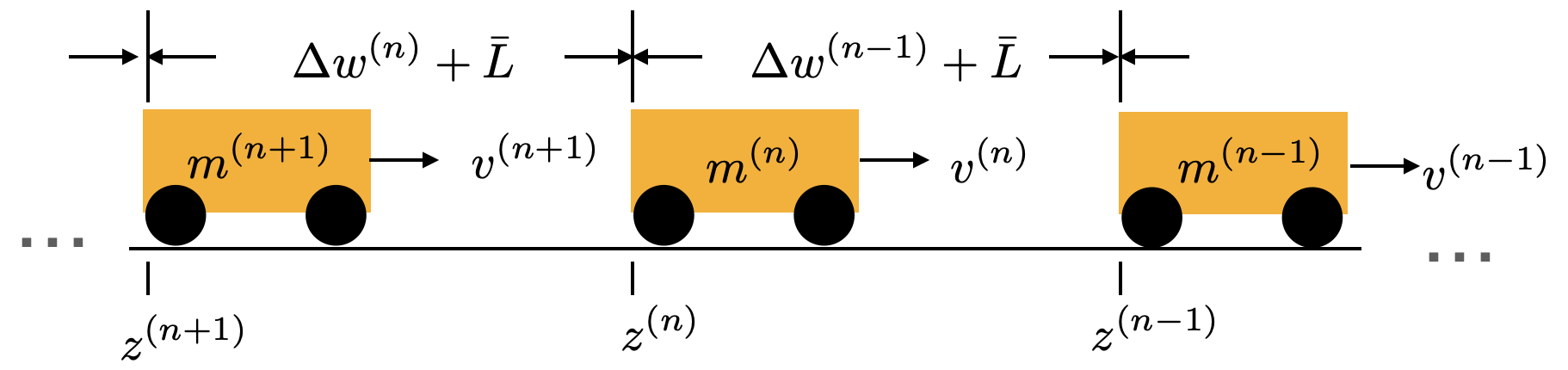
Figure 1: We focus on a scenario in which cars need to regulate to a specified gap $L$ at a desired reference velocity $v$. Deviations from the desired position are $\Delta w^{(n)}$ and deviations from the reference velocity are $\Delta v^{(n)}$.

We consider the problem of maintaining a fixed distance, $\bar{L}$, between $n$ cars at a desired velocity $v$ as depicted in Figure 1. We adapt the continuous-time dynamics for relative position as given in [18] to discrete-time dynamics with sampling time $T_{s}$:

$$\Delta v_{t+1}^{(n)} =\bigg{(}-\frac{\alpha^{(n)}T_{s}}{m^{(n)}}+1\bigg{)}\Delta v_{t}^{(n)}+\frac{T_{s}}{m^{(n)}}\Delta u_{t}^{(n)},$$ (22)

$$\Delta w_{t+1}^{(n)} =T_{s}(\Delta v_{t}^{(n)}-\Delta v_{t}^{(n+1)})+\Delta w_{k}^{(n)},$$ (23)

where $\Delta v^{(n)}$ is the deviation from the reference velocity at car $n$ and $\Delta w^{(n)}$ is the deviation of the gap between cars $n+1$ and $n$ from the desired gap $L$. $\Delta u$ is a change in force input for each car. This leads to an $n$ car state-vector $x_{t+1}:=[\Delta v_{t+1}^{(1)},\Delta w_{t+1}^{(1)},\Delta v_{t+1}^{(2)},...,\Delta v_{t+1}^{(n)}]^{T}$. As such $A$ and $B$ are given by:

$$A =\begin{bmatrix}-\frac{\alpha^{(1)}T_{s}}{m^{(1)}}+1&0&0&0&\ldots\\ T_{s}&1&-T_{s}&0&\ldots\\ 0&0&-\frac{\alpha^{(2)}T_{s}}{m^{(2)}}+1&0&\ldots\\ 0&0&T_{s}&1&\ldots\\ \vdots&\vdots&\vdots&\vdots&\ddots\end{bmatrix}$$ (24)

$$B =\begin{bmatrix}\frac{T_{s}}{m^{(1)}}&0&\ldots\\ 0&0&\ldots\\ 0&\frac{T_{s}}{m^{(2)}}&\ldots\\ 0&0&\ldots\\ \vdots&\vdots&\ddots\end{bmatrix}.$$ (25)

While there is a specific structure to $(A,B)$ here, we assume we do not know the structure and estimate all $(2n-1)(3n-1)$ entries. We specify the noise covariance in the dynamics (6) as $\Sigma_{w}=1\mathrm{e}{-2}\times I_{5}$. The prior on the parameters (9) is $\Theta_{0}=[A,B]$ with $m^{(1)}=m^{(2)}=m^{(3)}=1$, $\alpha^{(1)}=\alpha^{(2)}=\alpha^{(3)}=1$, $T_{s}=0.1$; $\lambda_{0}^{-1}=1\mathrm{e}{-2}\times I_{8}$. Horizon $N=30$.

V-B Experiment Design Setup

In the results that follow, we use an experiment horizon of $M=20$ time steps, and batch size $L=1000$ in Algorithm 1. As in [18], for the criteria in (7) $Q$ includes penalties of magnitude $10$ on the positions $\Delta w$ and zero on the velocity $\Delta v$. $R$ is the identity matrix. The weight matrix $S$ has parameters $\alpha_{1}=10^{3},\alpha_{2}=10^{6}$. $U$ is initialized with $u_{t}\sim U[10^{-}3,10^{-}2]$ and is fixed across experiments.

To solve the A-optimal experiment design in (5), we use a pathwise gradient estimator of the same form as (17) to perform stochastic gradient descent, where the objective is to minimize the trace of the posterior error covariance (9).

V-C Results and Discussion

We start by comparing the performance of our method against A-optimal design (5) in terms of post-experiment LQR control performance (7). For the experiment design (4), we consider a feasible input set $\mathcal{U}$ where the Frobenius norm of the input sequence, $U$, is bounded by a design parameter $\beta$ such that $\mathcal{U}=\left\{U\,|\,\|U\|_{F}\leq\beta\right\}$. We vary the allowed magnitude, $\beta$, in Figure 2 and observe our method outperforms the A-optimal design uniformly. For any experiment design, we have a lower and upper bound on the performance. If we knew the values of $(A,B)$, we would achieve the lowest possible control cost such that this is a lower bound on achievable performance. The upper bound comes from the expected control performance associated with using a controller that uses the a-priori system estimate instead of the a-posteriori as in (3). Intuitively, as the budget $\beta$ for an experiment increases, so should the experiment performance as the experiment can “explore more”. For small $\beta$ the methods are nearly comparable as the additional information in minimal, but as $\beta$ increases the performance of our method approaches that of the perfect knowledge case. The A-optimal design only slowly decreases even though in the limit it should reach the lower bound.

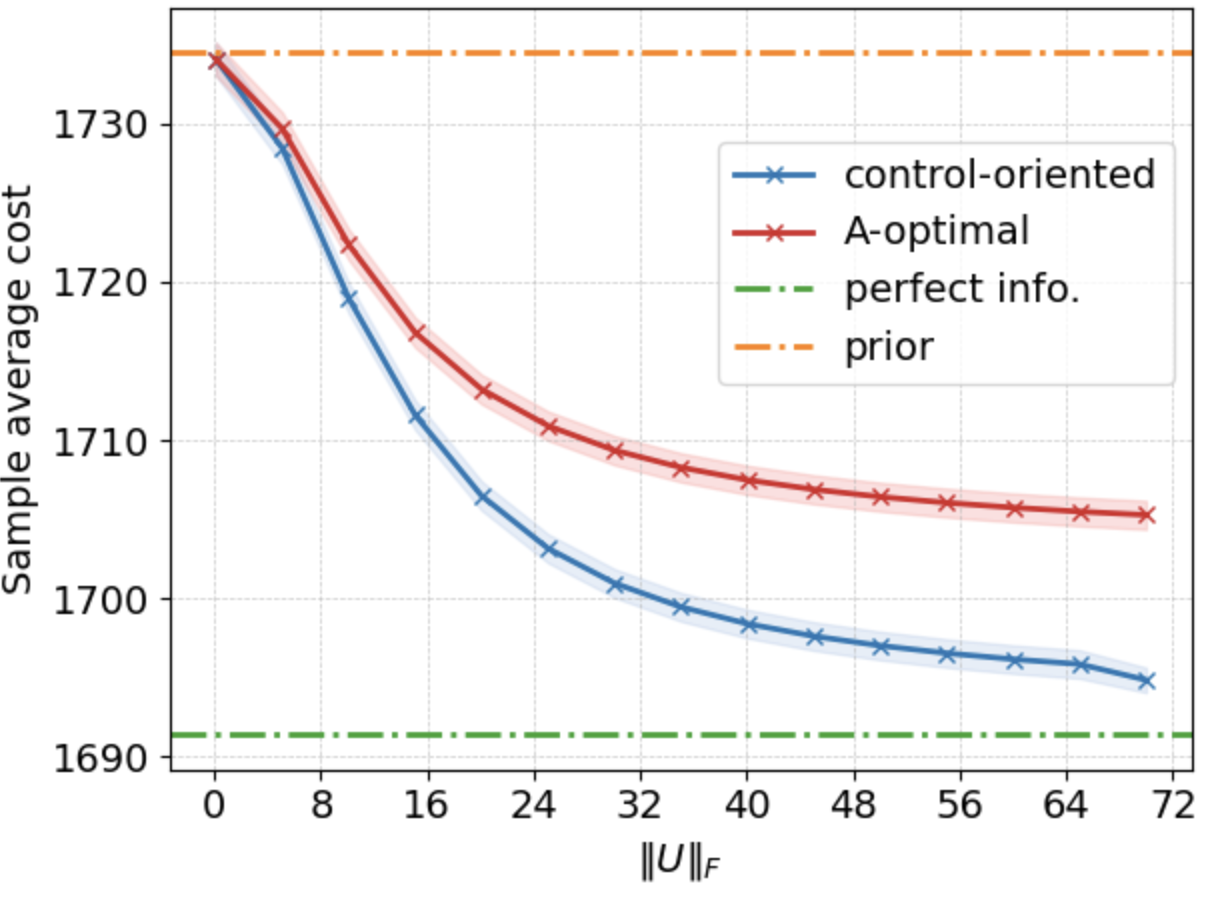
Figure 2: We compare the performance of our control-oriented system identification against A-optimal experiment design for a system with five states and three inputs, and known initial condition $x_{0}=[0.,-4.3,0.,2.1,2.5]^{T}$ as in [18]. Any experiment design performance is lower-bounded by the optimal control given knowledge of $(A,B)$ and upper bounded by the performance of the controller given the a-priori system estimate. We include 95$\%$ confidence intervals using $10^{5}$ samples.

In Figure 3, we observe the optimal experiment inputs ($\Delta u$) for a three-car system. The experiment inputs for our control-oriented approach exhibit more excitation over the time horizon than the A-optimal design, which has a relatively smooth experiment input sequence, suggesting our method would perform better, which is verified by Figure 2. We also consider what the input sequence would look like if the controller given the a-priori system estimate is used during an experiment trial. Since the controller is closed-loop (11), we show the average input sequence. Using the optimal control may seem like a natural way to conduct an experiment, but the norm bound $\beta$ on the input is not active in this case, indicating that simply performing the optimal control leaves experiment budget unused.

Figure 4 shows how the problem scales with the system dimension. In the first subplot we see the convergence of the experiment criteria in (4) as a function of iterations. The criteria is normalized by the lower bound (given by the performance if we knew $A,B$) for illustrative purposes. The number of iterations until the criteria stabilizes is roughly constant across problem dimension suggesting that the number of iterations required is independent of the system size in this case. In the second subplot, the time to compute each gradient sample is shown as a function of the state dimension. The compute time is dominated by “control solution”–the time to solve the LQR problem–thus suggesting that the time-complexity is dominated by the control problem. “Overhead” refers to the remainder of the compute tasks such as automatic differentiation and initialization of objects in the python library JAX [19].

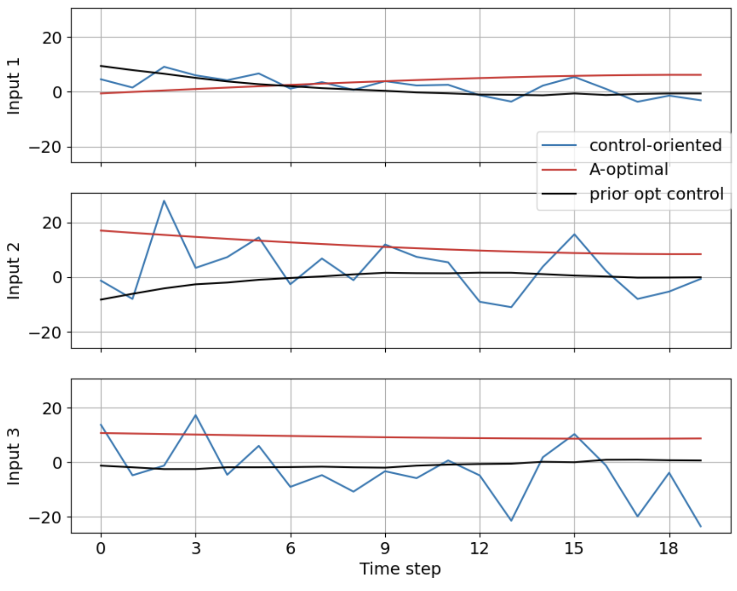
Figure 3: The experiment input sequences for each car in a 3 car system are compared under the proposed method, A-optimal experiment design, and by conducting the experiment with a feedback controller given the prior.

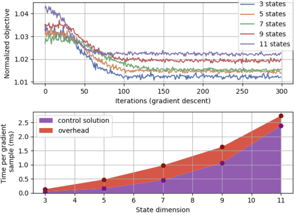
Figure 4: In the upper subplot, the number of iterations to converge for the car string problem is essentially the same regardless of system size suggesting good scaling properties of our method. In the lower subplot, we observe the average time to compute a single gradient sample. The time is dominated by solving the control problem and “overhead” refers to tasks such as automatic differentiation, initial compile time, etc.

VI Conclusion

We proposed a control-oriented identification approach that in expectation improves any data-driven controller by construction. Our solution method via stochastic gradient descent is shown in the LQR setting to provide solutions that outperform a typical experiment design objective in the sense that the post-experiment control performance is better with our method.

Our experiment design approach extends beyond the LQR setting, and it would be interesting to apply this to more general parametric problems. Establishing analytical results on the convergence rate and sample complexity of the stochastic gradient descent is an important direction for future research.

VII Appendix

VII-A Change of variable for linear system

We want to find a change of variable for the linear system (6). We start by showing the case for $t=2$ such that

$$x_{1} =Ax_{0}+Bu_{0}+w_{0}$$ (26a)

$$x_{2} =Ax_{1}+Bu_{1}+w_{1}$$ (26b)

and expressing $$x_{1} x_{0}$$ in terms of

$$=A^{2}x_{0}+ABu_{0}+Aw_{0}+Bu_{1}+w_{1}$$ (26c)

Then assuming this holds for time $$t$$:

$$x_{t}=A^{t}x_{0}+\sum_{l=0}^{t-1}A^{t-1-l}(Bu_{l}+w_{l}),$$ (26d)

at time $$t+1$$

$$x_{t+1} =Ax_{t}+Bu_{t}+w_{t}$$ (26e)

substituting the recursion (26d)

$$x_{t+1} =A(A^{t}x_{0}+\sum_{l=0}^{t-1}A^{t-1-l}(Bu_{l}+w_{l}))+B_{t}+w_{t},$$ (26f)

$$x_{t+1} =A^{t+1}x_{0}+\sum_{l=0}^{t}A^{t-l}(Bu_{l}+w_{l}),$$ (26g)

the desired result, where $w_{t}$ is distributed according to the process noise and is independent of $u_{t}$.

VII-B Differentiability of the value function

Here we show the value function is differentiable with respect to the decision variable $U$. In particular, with $\pi:=\{K_{0},...,K_{N-1}\}$ we write the gradient as

$$\partialderivative{J}{u_{ij}}=\sum\partialderivative{J}{K_{t,k,l}}\partialderivative{K_{t,k,l}}{\hat{{\Theta}}_{m,n}}\partialderivative{\hat{\Theta}_{m,n}}{u_{ij}}$$ (27)

VII-B1 Gradient of $J$ with respect to $K_{t}$

First, we observe that the gradient of (12a) at $t=0$ is given by

$$\partialderivative{J}{K_{0}} =2\big{(}(R+B^{T}P_{1}B)K_{0}+B^{T}P_{1}A\big{)}x_{0}x_{0}^{T}$$ (28a)

and for $$t>0$$ as

$$\begin{split}&\partialderivative{J}{K_{t}}=2\big{[}(R+B^{T}P_{t+1}B)K_{t}+B^{T}P_{t+1}A\big{]}\\ &\times\bigg{(}\Pi_{i=0}^{t-1}(A+BK_{i})x_{0}x_{0}^{T}\Pi_{i=t-1}^{0}(A+BK_{i})^{T}+\Sigma_{w}\\ &+\sum_{j=1,t>1}^{t-1}\Pi_{i=j}^{t-1}(A+BK_{i})\Sigma_{w}\Pi_{i=t-1}^{j}(A+BK_{i})^{T}\bigg{)}\end{split}$$ (28b)

For a finite horizon, the entries of $P_{t}$ are finite even if the cost grows exponentially in time such that the gradient itself will be finite. Furthermore, the the gradient is polynomial in the Gaussian random variables $(A,B)$ such that there exists a polynomial function of the random variables, which is integrable.

VII-B2 Derivation: Gradient of $J$ with respect to $K_{t}$

We want to take the gradient of the value function

$$J(\Theta,\pi):=x_{0}^{T}P_{0}x_{0}+\sum_{t=0}^{N-1}\tr(P_{t+1}\Sigma_{W})$$ (29a)

with respect to $$K_{t} K_{0} P_{0}$$. For we expand to see the dependence

$$\begin{split}&\partialderivative{J(\Theta,\pi)}{K_{0}}=\partialderivative{K_{0}}\bigg{(}x_{0}^{T}(Q+K_{0}^{T}RK_{0}+\\ &(A+BK_{0})^{T}P_{1}(A+BK_{0})x_{0}+\sum_{t=0}^{N-1}\tr(P_{t+1}\Sigma_{W})\bigg{)}.\end{split}$$ (29b)

Evaluting this, we get

$$\partialderivative{J(\Theta,\pi)}{K_{0}}=(2RK_{0}+2B^{T}P_{1}BK_{0})x_{0}x_{0}^{T}+2B^{T}P_{1}Ax_{0}x_{0}^{T},$$ (29c)

which can be rearranged to give the desired result. For $$t>0 P_{i} i=t K_{0} x_{t}:=\Pi_{i=0}^{t-1}(A+BK_{i})x_{0}$$, there is dependence in both the initial condition and the process noise term. For the initial condition term, recursively expand until , and then take the gradient as for . If we define the current state as , then we can express this relationship as

$$\partialderivative{(x_{0}^{T}P_{0}x_{0})}{K_{t}}=2\big{[}(R+B^{T}P_{t+1}B)K_{t}+B^{T}P_{t+1}A\big{]}x_{t}x_{t}^{T}.$$ (29d)

This gives us the first part of the gradient. The second part is due to the process noise and follows a similar pattern. Start by expanding $$P_{t+1} K_{t+1}$$ to get terms of :

$$\begin{split}&\tr(P_{t}\Sigma_{w})=\\ &\tr\big((Q+K_{t}^{T}RK_{t}+(A+BK_{t})^{T}P_{t+1}(A+BK_{t}))\Sigma_{w}\big{missing})\end{split}$$ (29e)

Expanding $$P_{t+1} t$$, we need to take gradients of the following terms (here given at ):

$$\partialderivative{K_{t}}\tr(K_{t}\Sigma K_{t}^{T}R)=2RK_{t}\Sigma_{w}.$$ (29f)

$$\partialderivative{K_{t}}\tr(K_{t}\Sigma_{w}K_{t}^{T}B^{T}P_{t+1}B)=2B^{T}P_{t+1}BK_{t}\Sigma_{w}.$$ (29g)

$$\partialderivative{K_{t}}2\tr(\Sigma_{w}A^{T}P_{t+1}BK_{t})=2B^{T}P_{t+1}A\Sigma_{w}.$$ (29h)

Using these gradients and algebraic manipulations, we get the desired result for one step for the process noise term. This can be repeated for all time steps to get the overall result. Combining the initial condition terms with the noise terms gives us the gradient for $t>0$.

VII-B3 Gradient of $K_{t}$ with respect to estimate $\Theta$

Next, we examine the gradient of the data-driven control with respect to the estimated system, denoted above as $(\hat{A},\hat{B})$ as we use certainty equivalence in the dynamics parameters. The gradient of

$$K_{t}=-(R+\hat{B}^{T}P_{t+1}\hat{B})^{-1}\hat{B}^{T}P_{t+1}\hat{A}$$ (30a)

with respect to $$\hat{\Theta} \hat{A},\hat{B}$$ is most easily written in terms of the elements of .

The gradient is recursively computed as

$$\begin{split}\partialderivative{K_{t}}{A_{ij}}&=(R+B^{T}P_{t+1}B)^{-1}B^{T}\partialderivative{P_{t+1}}{A_{ij}}B(R+B^{T}P_{t+1}B)^{-1}\\ &-(R+B^{T}P_{t+1}B)^{-1}\bigg{(}B^{T}\partialderivative{P_{t+1}}{A_{ij}}A+B^{T}P_{t+1}e_{ij}\bigg{)}\end{split}$$ (30b)

$$\begin{split}\partialderivative{K_{t}}{B_{ij}}&=(R+B^{T}P_{t+1}B)^{-1}\bigg{(}2e_{ij}^{T}P_{t+1}B+B^{T}\partialderivative{P_{t+1}}{B_{ij}}B\bigg{)}\\ &\times(R+B^{T}P_{t+1}B)^{-1}\\ &-(R+B^{T}P_{t+1}B)^{-1}\bigg{(}B^{T}\partialderivative{P_{t+1}}{B_{ij}}B+2e_{ij}^{T}P_{t+1}B\bigg{)}\end{split}$$ (30c)

with

$$\begin{split}\partialderivative{P_{t}}{A_{ij}}&=2\partialderivative{K_{t}}{A_{ij}}^{T}RK_{t}+A^{T}\partialderivative{P_{t+1}}{A_{ij}}A\\ &+2e_{ij}^{T}P_{t+1}A+2e_{ij}^{T}P_{t+1}BK_{t}\\ &+2A^{T}\partialderivative{P_{t+1}}{A_{ij}}BK_{t}+2A^{T}P_{t+1}B\partialderivative{K_{t}}{A_{ij}}\\ &+2\partialderivative{K_{t}}{A_{ij}}^{T}B^{T}P_{t+1}BK_{t}+K_{t}^{T}B^{T}\partialderivative{P_{t+1}}{A_{ij}}BK_{t}\end{split}$$ (30d)

$$\begin{split}\partialderivative{P_{t}}{B_{ij}}&=2\partialderivative{K_{t}}{B_{ij}}^{T}RK_{t}+A^{T}\partialderivative{P_{t+1}}{B_{ij}}A+2A^{T}P_{t+1}e_{ij}K_{t}\\ &+2A^{T}\partialderivative{P_{t+1}}{B_{ij}}BK_{t}+2A^{T}P_{t+1}B\partialderivative{K_{t}}{B_{ij}}\\ &+2\partialderivative{K_{t}}{B_{ij}}^{T}B^{T}P_{t+1}BK_{t}+K_{t}^{T}B^{T}\partialderivative{P_{t+1}}{B_{ij}}BK_{t}\\ &+2K_{t}^{T}e_{ij}^{T}P_{t+1}BK_{t}.\end{split}$$ (30e)

with $P_{N}=Q_{N}$. Again, we appeal to the fact that the elements of $P_{t}$ as governed by (11) will be finite for a finite horizon, leading to finite values for the gradients. Furthermore, the gradient is again polynomial in the parameters such that there exists a polynomial function that upper bounds the gradient and is integrable.

VII-B4 Derivation: Gradient of $K_{t}$ with respect to estimate $\Theta$

For a posterior distribution with mean $\hat{\Theta}=[\hat{A},\hat{B}]$, and the controller defined by the Riccati difference equations:

$$K_{t} =-(R+\hat{B}^{T}P_{t+1}\hat{B})^{-1}\hat{B}^{T}P_{t+1}\hat{A},$$ (31a)

$$P_{t} =Q+K_{t}^{T}RK_{t}-(\hat{A}+\hat{B}K_{t})^{T}P_{t+1}(\hat{A}+\hat{B}K_{t}),$$ (31b)

we want to find the gradient with respect to elements of $\hat{A}$ and $\hat{B}$. Starting with $K_{t}$:

$$\partialderivative{K_{t}}{\hat{A}_{ij}} =\partialderivative{\hat{A}_{ij}}\bigg{(}-(R+\hat{B}^{T}P_{t+1}\hat{B})^{-1}\hat{B}^{T}P_{t+1}\hat{A}\bigg{)}$$ (32a)

$$\begin{split}&=\partialderivative{\hat{A}_{ij}}\big{(}-(R+\hat{B}^{T}P_{t+1}\hat{B})^{-1}\big{)}\hat{B}^{T}P_{t+1}\hat{A}\\ &+\big{(}-(R+\hat{B}^{T}P_{t+1}\hat{B})^{-1}\big{)}\partialderivative{\hat{A}_{ij}}\big{(}\hat{B}^{T}P_{t+1}\hat{A}\big{)}\end{split}$$ (32b)

For the gradient of the first component:

$$\partialderivative{\hat{A}_{ij}}\big{(}-(R+\hat{B}^{T}P_{t+1}\hat{B})^{-1}\big{)}=$$ (32c)

$$(R+\hat{B}^{T}P_{t+1}\hat{B})^{-1}\partialderivative{(R+\hat{B}^{T}P_{t+1}\hat{B})}{\hat{A}_{ij}}\big{(}(R+\hat{B}^{T}P_{t+1}\hat{B})^{-1}\big{)}$$ (32d)

$$=(R+\hat{B}^{T}P_{t+1}\hat{B})^{-1}\hat{B}^{T}\partialderivative{P_{t+1}}{\hat{A}_{ij}}\hat{B}\big{(}(R+\hat{B}^{T}P_{t+1}\hat{B})^{-1}\big{)}$$ (32e)

and the second

$$\partialderivative{\hat{A}_{ij}}\big{(}\hat{B}^{T}P_{t+1}\hat{A}\big{)}=\hat{B}^{T}\bigg{(}\partialderivative{P_{t+1}}{\hat{A}_{ij}}\hat{A}+P_{t+1}e_{ij}\bigg{)}.$$ (32f)

The results for the partial with respect to $$B_{ij} P_{t}$$ follows similarly. In each case, we need to compute the partial of :

$$\begin{split}&\partialderivative{P_{t}}{\hat{A}_{ij}}=\\ &\partialderivative{\hat{A}_{ij}}\big{(}Q+K_{t}^{T}RK_{t}-(\hat{A}+\hat{B}K_{t})^{T}P_{t+1}(\hat{A}+\hat{B}K_{t})\big{)}.\end{split}$$ (32g)

$$Q \hat{A} \hat{B}$$ is independent of (and ). The rest of terms are:

$$\partialderivative{\hat{A}_{ij}}\big{(}K_{t}^{T}RK_{t}\big{)}=2\partialderivative{K_{t}}{\hat{A}_{ij}}^{T}RK_{t},$$ (32h)

$$\partialderivative{\hat{A}_{ij}}\big{(}(\hat{A}+\hat{B}K_{t})^{T}P_{t+1}(\hat{A}+\hat{B}K_{t})\big{)}=$$ (32i)

$$2e_{ij}^{T}P_{t+1}\hat{A}+\hat{A}^{T}\partialderivative{P_{t+1}}{\hat{A}_{ij}}\hat{A}+\partialderivative{\hat{A}_{ij}}\big{(}\hat{A}^{T}P_{t+1}\hat{B}K_{t}\big{)},$$ (32j)

and

$$\begin{split}&\partialderivative{\hat{A}_{ij}}\big{(}\hat{A}^{T}P_{t+1}\hat{B}K_{t}\big{)}=2e_{ij}^{T}P_{T+1}\hat{B}K_{t}\\ &+2\hat{A}^{T}\partialderivative{P_{t+1}}{\hat{A}_{ij}}\hat{B}K_{t}+2\hat{A}^{T}P_{t+1}\hat{B}\partialderivative{K_{t}}{\hat{A}_{ij}},\end{split}$$ (32k)

A similar derivation follows with respect to $$\hat{B}_{ij}$$.

VII-B5 Gradient of estimate $\Theta$ with respect to $U$ with derivation

Finally, to address the gradient of the estimated value with respect to the design variable $U\in\mathbb{R}^{n_{u}\times T}$ with entries $u_{ij}$, we first rewrite the estimator in (9) using sums as

$$\hat{\Theta} =(\Theta_{0}\Lambda_{0}+\sum_{t=0}^{T-1}y_{t}s_{t}z_{t}^{T})(\Lambda_{0}+\sum_{t=0}^{T-1}z_{t}s_{t}z_{t}^{T})^{-1},$$ (33a)

$$=:\Psi\Delta,$$ (33b)

where

$$y_{t} =x_{t+1}=Ax_{t}+B\gamma_{t},$$ (33c)

$$x_{t} =A^{t}x_{0}+\sum_{l=0}^{t-1}A^{t-1-l}(Bu_{l}+w_{l}),$$ (33d)

$$z_{t} =[x_{t};u_{t}].$$ (33e)

$y_{t},s_{t},z_{t}$ all depend on $U$. We use the $\mathrm{vec}\left(\right)$ operator, which stacks the columns on tops of each other, to simplify the derivation. As such,

$$\begin{split}\mathrm{vec}\left(\partialderivative{\hat{\Theta}}{u_{ij}}\right)&=(\Delta^{T}\otimes I)\mathrm{vec}\left(\partialderivative{\Psi}{u_{ij}}\right)+(I\otimes\Psi)\mathrm{vec}\left(\partialderivative{\Delta}{u_{ij}}\right),\end{split}$$ (33f)

where

$$\begin{split}&\mathrm{vec}\left(\partialderivative{\Psi}{u_{ij}}\right)=\\ &\mathrm{vec}\left(\partialderivative{\sum_{t=0}^{T-1}y_{t}s_{t}z_{t}^{T}}{u_{ij}}\right)=\sum_{t=0}^{T-1}\mathrm{vec}\left(\partialderivative{y_{t}s_{t}z_{t}^{T}}{u_{ij}}\right),\\ &=(z_{t}s_{t}^{T}\otimes I)\mathrm{vec}\left(\partialderivative{y_{t}}{u_{ij}}\right)+(z_{t}\otimes y_{t})\mathrm{vec}\left(\partialderivative{s_{t}}{u_{ij}}\right)\\ &+(I\otimes y_{t}s_{t})\mathrm{vec}\left(\partialderivative{z_{t}^{T}}{u_{ij}}\right).\end{split}$$ (33g)

Each gradient in the above expression is

$$\begin{split}\mathrm{vec}\left(\partialderivative{y_{t}}{u_{ij}}\right)&=\mathrm{vec}\left(\partialderivative{u_{ij}}A^{t+1}x_{0}+\sum_{l=0}^{t}A^{t-l}(B\gamma_{l}+w_{l})\right),\\ &=\sum_{l=0}^{t}(I\otimes A^{t-l}B)\mathrm{vec}\left(\partialderivative{\gamma_{l}}{u_{ij}}\right),\\ &=(I\otimes A^{t-i}B)\mathrm{vec}\left(e_{ij}\right),\quad(t\geq i)\end{split}$$ (33h)

$$\begin{split}&\mathrm{vec}\left(\partialderivative{s_{t}}{u_{ij}}\right)=\mathrm{vec}\left(\partialderivative{u_{ij}}\atan((\norm{x_{t}}-\alpha_{1})\alpha_{2})/\pi+0.5\right)\\ &=\mathrm{vec}\left(\frac{1}{\pi\alpha_{2}^{2}}\frac{1}{1/\alpha_{2}^{2}+(\norm{x_{t}}-\alpha_{1})^{2}}\partialderivative{u_{ij}}\big{(}(\norm{x_{t}}-\alpha_{1})^{2}\big{)}\right)\\ &\partialderivative{u_{ij}}\big{(}(\norm{x_{t}}-\alpha_{1})^{2}\big{)}=2(\norm{x_{t}}-\alpha_{1})\frac{x_{t}}{\norm{x_{t}}}\partialderivative{x_{t}}{u_{ij}}\end{split}$$ (33i)

$$\begin{split}&\mathrm{vec}\left(\partialderivative{z_{t}^{T}}{u_{ij}}\right)=\\ &\mathrm{vec}\left(\partialderivative{u_{ij}}\begin{bmatrix}A^{t}x_{0}+\sum_{l=0}^{t-1}A^{t-1-l}(Bu_{l}+w_{l})\\ u_{t}\end{bmatrix}^{T}\right)\\ &=\begin{bmatrix}(I\otimes A^{t-1-i}B)\mathrm{vec}\left(\partialderivative{u_{i}}{u_{ij}}\right),\quad(t\geq i)\text{ else 0}\\ \mathrm{vec}\left(e_{ij}\right),\quad(i=t),\text{ else 0}\end{bmatrix}^{T}\end{split}$$ (33j)

Going to the second term, $\Delta$, in the estimator, we obtain

$$\mathrm{vec}\left(\partialderivative{\Delta}{u_{ij}}\right)=-(\Delta\otimes\Delta)\mathrm{vec}\left(\partialderivative{u_{ij}}\sum_{t=0}^{T-1}z_{t}s_{t}z_{t}^{T}\right)$$ (33k)

$$=-(\Delta\otimes\Delta)\sum_{t=0}^{T-1}\Bigg{(}(z_{t}s_{t}^{T}\otimes I)$$ (33l)

$$\times\begin{bmatrix}(I\otimes A^{t-1-i}B)\mathrm{vec}\left(e_{ij}\right),\leavevmode\nobreak\ (t\geq j),\text{else 0}\\ \mathrm{vec}\left(e_{ij}\right),\leavevmode\nobreak\ (j=t),\text{else 0}\end{bmatrix}$$ (33m)

$$+(z_{t}\otimes z_{t})\mathrm{vec}\left(\partialderivative{s_{t}}{\gamma_{i}}\right)+(I\otimes Z_{T}s_{t})$$ (33n)

$$\times\begin{bmatrix}(I\otimes A^{t-1-i}B)\mathrm{vec}\left(e_{ij}\right),\leavevmode\nobreak\ (t\geq j),\text{else 0}\\ \mathrm{vec}\left(e_{ij}\right),\leavevmode\nobreak\ (i=t),\text{else 0}\end{bmatrix}^{T}\Bigg{)}$$ (33o)

The gradient is then well-defined except if $\Delta$ were to be ill-defined due to lack of invertibility; however, the prior $\Lambda_{0}$ is chosen to be non-singular and obviates this possibility. The resulting expression contains a rational and polynomial term, such that there exists a polynomial bounding function. Overall then, for each term in the gradient, there exists an integrable bounding function such that the dominated convergence can be applied and the exchange of gradient (limit) and integral is valid.

References

- [1] H. Chernoff, “Locally Optimal Designs for Estimating Parameters,” The Annals of Mathematical Statistics, vol. 24, no. 4, pp. 586–602, Dec. 1953, publisher: Institute of Mathematical Statistics.
- [2] H. A. Simon, “Dynamic Programming Under Uncertainty with a Quadratic Criterion Function,” Econometrica, vol. 24, no. 1, pp. 74–81, 1956, publisher: [Wiley, Econometric Society].
- [3] G. Elfving, “Optimum Allocation in Linear Regression Theory,” The Annals of Mathematical Statistics, vol. 23, no. 2, pp. 255–262, Jun. 1952, publisher: Institute of Mathematical Statistics.
- [4] K. Lindqvist and H. Hjalmarsson, “Identification for control: adaptive input design using convex optimization,” in Proceedings of the 40th IEEE Conference on Decision and Control (Cat. No.01CH37228), vol. 5. Orlando, FL, USA: IEEE, 2001, pp. 4326–4331.
- [5] M. Gevers, “Identification for Control: From the Early Achievements to the Revival of Experiment Design,” in Proceedings of the 44th IEEE Conference on Decision and Control, Dec. 2005, pp. 12–12, iSSN: 0191-2216.
- [6] S. Anderson, K. Byl, and J. P. Hespanha, “Experiment design with gaussian process regression with applications to chance-constrained control,” in 2023 62nd IEEE Conference on Decision and Control (CDC), 2023, pp. 3931–3938.
- [7] B. D. Lee, I. Ziemann, A. Tsiamis, H. Sandberg, and N. Matni, “The Fundamental Limitations of Learning Linear-Quadratic Regulators,” Mar. 2023, arXiv:2303.15637 [cs, eess].
- [8] A. J. Wagenmaker, M. Simchowitz, and K. Jamieson, “Task-Optimal Exploration in Linear Dynamical Systems,” in Proceedings of the 38th International Conference on Machine Learning. PMLR, Jul. 2021, pp. 10 641–10 652, iSSN: 2640-3498.
- [9] S. Dean, H. Mania, N. Matni, B. Recht, and S. Tu, “On the Sample Complexity of the Linear Quadratic Regulator,” Foundations of Computational Mathematics, vol. 20, no. 4, pp. 633–679, Aug. 2020.
- [10] K. J. Åström and B. Wittenmark, Adaptive control. Courier Corporation, 2008.
- [11] M. Simchowitz and D. Foster, “Naive Exploration is Optimal for Online LQR,” in Proceedings of the 37th International Conference on Machine Learning. PMLR, Nov. 2020, pp. 8937–8948, iSSN: 2640-3498.
- [12] S. Mohamed, M. Rosca, M. Figurnov, and A. Mnih, “Monte Carlo Gradient Estimation in Machine Learning,” Sep. 2020.
- [13] J. Peters and S. Schaal, “Reinforcement learning of motor skills with policy gradients,” Neural Networks, vol. 21, no. 4, pp. 682–697, May 2008.
- [14] P. Rossi, G. Allenby, and R. McCulloch, Bayesian Statistics and Marketing. Wiley, Oct. 2006.
- [15] D. Bertsekas, Dynamic programming and optimal control: Volume I. Athena scientific, 2012, vol. 4.
- [16] P. Glasserman, Monte Carlo methods in financial engineering. Springer, 2004, vol. 53.
- [17] G. Grimmett and D. Stirzaker, Probability and random processes. Oxford university press, 2020.
- [18] W. Levine and M. Athans, “On the optimal error regulation of a string of moving vehicles,” IEEE Transactions on Automatic Control, vol. 11, no. 3, pp. 355–361, Jul. 1966, conference Name: IEEE Transactions on Automatic Control.
- [19] “JAX: Autograd and XLA,” Feb. 2023, original-date: 2018-10-25T21:25:02Z.