Exploiting polar symmetry in designing equivariant observers for vision-based motion estimation

Abstract

Accurately estimating camera motion from image sequences poses a significant challenge in computer vision and robotics. Many computer vision methods first compute the essential matrix associated with a motion and then extract orientation and normalized translation as inputs to pose estimation, reconstructing the scene scale (that is unobservable in the epipolar construction) from separate information. In this paper, we design a continuous-time filter that exploits the same perspective by using the epipolar constraint to define pseudo-measurements. We propose a novel polar symmetry on the pose of the camera that makes these measurements equivariant. This allows us to apply recent results from equivariant systems theory to estimating pose. We provide a novel explicit persistence of excitation condition to characterize observability of the full pose, ensuring reconstruction of the scale parameter that is not directly observable in the epipolar construction.

1 Introduction

Accurately estimating the motion of a camera from visual data is a fundamental challenge in robotics and computer vision. The problem is key to a range of applications including visual odometry, target tracking, 3D scene reconstruction, etc. One of the key ideas in classical computer vision used in extracting motion information from a video sequence relies on computing the so-called essential matrix between consecutive images Longuet-Higgins (1981). The essential matrix relates pairs of associated image points between two images taken by the same camera as it moves in the scene Hartley and Zisserman (2003). The essential matrix can be computed from a set of at least five Nistér (2004) (or eight Hartley (1997)) matched image points, although in practice it is usually computed using nonlinear optimization over many image points Ma et al. (2001); Botterill et al. (2011). The essential matrix captures the essential information of the camera motion available from the visual feed.

Once the essential matrix is obtained, it can be decomposed into a rotation and a normalized translation, leading to four possible pairs of translations and rotations Hartley and Zisserman (2003). The correct pair can be identified through a chirality check, ensuring that corresponding features are visible in front of both cameras. The resulting pose estimation has the correct rotation and a normalized translation, that is a direction of translation. The actual magnitude of the camera translation is linked to estimation of the scene scale and is unobservable for the image sequence alone, depending on some additional measurements and a separate motion estimation process.

Filter-based algorithms are most effective when they are posed directly on measurements, image points in this case, rather than derived information such as an essential matrix estimation. Recent work White and Beard (2020) introduced an iterative algorithm that optimizes rotation and normalized translation between frames to compute relative pose based on minimizing the epipolar constraint. In parallel, Hua et al. (2020) proposed a deterministic Riccati observer that involves velocity measurements and uses the epipolar constraint to define a pseudo-measurement Julier and LaViola (2007) to estimate the camera pose directly. In Hua et al. (2020), and a following paper Gintrand et al. (2022), an observability analysis is provided to show that uniform observability is guaranteed provided that the translational motion of the camera is sufficiently exciting.

In this paper, we revisit the problem of designing a filter to estimate the motion of a camera by exploiting the epipolar constraint as a pseudo-measurement. We propose a new symmetry ${\mathbf{SO}}(3)\times\mathbf{SOT}(3)$ for the camera pose that we term the polar symmetry using the scaled orthogonal transformations Lie group $\mathbf{SOT}(3)$ van Goor et al. (2019). This symmetry is ideally suited to dealing with systems with unknown scale and was first proposed to model landmarks with bearing only visual measurements van Goor et al. (2019). For the first time (to the authors understanding) we apply the polar symmetry to the translation of the system pose. This allows us to demonstrate equivariance of the pseudo-measurement associated with the epipolar constraint. Moreover, we demonstrate equivariance of the system kinematics for measured velocity and from this determine a lifted system on the symmetry group. The following observer construction is based on the equivariant filter (EqF) methodology van Goor et al. (2020, 2023). Convergence of the filter depends on excitation of the velocity signal and we provide a comprehensive theoretical analyses of observability and stability. The resulting algorithm provides a powerful tool for tracking camera pose from visual data in the case where the velocity is measured.

The remainder of this paper is organized as follows. The notation and preliminaries are defined in Section 2. The problem is formally stated in Section 3 and the proposed equivariant observer is derived in Section 4. The observability and stability analysis is provided in Section 5. Simulation results are presented in Section 6 followed by concluding remarks in Section 7.

2 Preliminaries

2.1 Mathematical notation

Let $\mathcal{M}$ be a smooth manifold, $\mathrm{T}_{\xi}\mathcal{M}$ denotes the tangent space at $\xi\in\mathcal{M}$. Given a differentiable function between smooth manifolds $h:\mathcal{M}\rightarrow\mathcal{N}$, its differential at $\xi_{0}$ is written as

$$\mathrm{D}_{\xi}|_{\xi_{0}}h(\xi):\mathrm{T}_{\xi_{0}}\mathcal{M}\rightarrow\mathrm{T}_{\xi_{0}}\mathcal{N}.$$

Let $f:\mathcal{M}\rightarrow\mathcal{N}$ and $g:\mathcal{N}\rightarrow\mathcal{N}^{\prime}$ be linear maps, $f\cdot g$ denotes the composition of $f$ and $g$.

Let $\mathbf{G}$ be a matrix Lie group and $\mathfrak{g}$ its Lie algebra. The group identity is denoted ${\text{id}}\in\mathbf{G}$, left and right translation are written $L_{X}(Y):=XY$ and $R_{X}(Y):=YX,$ respectively, which induce the corresponding mappings on $\mathfrak{g}$, $\mathrm{d}L_{X}:\mathfrak{g}\rightarrow\mathrm{T}_{X}\mathbf{G}$ and $\mathrm{d}R_{X}:\mathfrak{g}\rightarrow\mathrm{T}_{X}\mathbf{G}$, defined by $\mathrm{d}L_{X}U:=XU$ and $\mathrm{d}R_{X}U:=UX$, respectively. The Adjoint map ${\text{Ad}}:\mathbf{G}\times\mathfrak{g}\rightarrow\mathfrak{g}$ is defined by ${\text{Ad}}_{X}(U):=XUX^{-1}$ for any $X\in\mathbf{G}$ and $U\in\mathfrak{g}$.

The Lie algebra $\mathfrak{g}$ is isomorphic to a vector space ${\mathbb{R}}^{\dim\mathfrak{g}}$. The wedge $(\cdot)^{\wedge}_{\mathfrak{g}}:{\mathbb{R}}^{\dim\mathfrak{g}}\rightarrow\mathfrak{g}$ and vee $(\cdot)^{\vee}_{\mathfrak{g}}:\mathfrak{g}\rightarrow{\mathbb{R}}^{\dim\mathfrak{g}}$ operators are linear isomorphisms that satisfy $(u^{\vee})^{\wedge}=u$ for all $u\in\mathfrak{g}$. The exponential map $\exp:\mathfrak{g}\rightarrow\mathbf{G}$ defines a local diffeomorphism from a neighborhood of $0\in\mathfrak{g}$ to a neighborhood of ${\text{id}}\in\mathbf{G}$, and its inverse (when defined) is the logarithmic map $\log:\mathbf{G}\rightarrow\mathfrak{g}$.

The $\mathbf{G}$-torsor, denoted $\mathcal{G}$, is defined as the set of elements of $\mathbf{G}$ (underlying manifold), but without the group structure.

A right group action is a smooth map $\phi:\mathbf{G}\times\mathcal{M}\rightarrow\mathcal{M}$ that satisfies the compatibility and identity properties

$$\phi\left(Y,\phi(X,\xi)\right) =\phi\left(XY,\xi\right), \phi({\text{id}},\xi) =\xi,$$

for all $\xi\in\mathcal{M}$ and $X\in\mathbf{G}$. For any $\xi\in\mathcal{M}$ the partial maps $\phi_{X}:\mathcal{M}\rightarrow\mathcal{M}$ and $\phi_{\xi}:\mathbf{G}\rightarrow\mathcal{M}$ are defined as $\phi_{X}(\xi):=\phi(X,\xi)$ and $\phi_{\xi}(X):=\phi(X,\xi)$, respectively. A group action is called transitive if for all $\xi_{1},\xi_{2}\in\mathcal{M}$, there exists $X\in\mathbf{G}$ such that $\phi(X,\xi_{1})=\xi_{2}$.

The special orthogonal group of 3D rotations is denoted by ${\mathbf{SO}}(3)$ with Lie algebra $\mathfrak{so}(3)$. They are defined by

$${\mathbf{SO}}(3) :=\{R\in{\mathbb{R}}^{3\times 3}\;|\;RR^{\top}=R^{\top}R=I_{3},\det(R)=1\},$$

$$\mathfrak{so}(3) :=\{a^{\times}\;|\;a\in{\mathbb{R}}^{3}\},\;a^{\times}:=\begin{pmatrix}0&-a_{3}&a_{2}\\ a_{3}&0&-a_{1}\\ -a_{2}&a_{1}&0\end{pmatrix},$$

where $a^{\times}$ denotes the skew-symmetric matrix associated with the vector (cross) product, satisfying $a^{\times}b=a\times b$ for all $b\in{\mathbb{R}}^{3}$. For any $a\in{\mathbb{R}}^{3}$, $a_{\mathfrak{so}(3)}^{\wedge}=a^{\times}$.

The scaled orthogonal transformations group denoted by $\mathbf{SOT}(3)$, with Lie algebra $\mathfrak{sot}(3)$, is the direct product of ${\mathbf{SO}}(3)$ and the multiplicative positive real numbers $\mathbf{MR}(1)=\{r\in{\mathbb{R}}\;|\;r>0\}$. They are defined by

$$\mathbf{SOT}(3) :=\{rQ\;|\;Q\in{\mathbf{SO}}(3),r>0\},$$

$$\mathfrak{sot}(3) :=\left\{\left(a,b\right)^{\wedge}_{\mathfrak{sot}(3)}\;|\;a\in{\mathbb{R}}^{3},b\in{\mathbb{R}}\right\},$$

$$\left(a,b\right)^{\wedge}_{\mathfrak{sot}(3)} :=a^{\times}+bI_{3}.$$

Denote the $2$-sphere by ${\mathbb{S}}^{2}:=\{p\in{\mathbb{R}}^{3}\mid|p|=1\}$, ${\mathbf{e}}_{1},{\mathbf{e}}_{2},{\mathbf{e}}_{3}$ denotes the canonical basis of ${\mathbb{R}}^{3}$ and ${\mathbb{S}}^{+}(k)$ denotes the set of positive definite $(k\times k)$ matrices.

For any $u\in{\mathbb{R}}^{3}\backslash\{0\}$ the projector $\Pi_{u}$ that projects vectors onto the subspace of ${\mathbb{R}}^{3}$ orthogonal to $u$ is given by

$$\Pi_{u}:=I_{3}-\frac{uu^{\top}}{|u|^{2}}=-\frac{u^{\times}u^{\times}}{|u|^{2}}.$$

2.2 Uniform observability of linear time-varying systems

Consider the following linear time-varying (LTV) system

$$\begin{cases}\dot{\mathbf{x}}=A(t)\mathbf{x}+B(t)\mathbf{u},\\ \mathbf{y}=C(t)\mathbf{x}\end{cases}$$ (1)

with state $\mathbf{x}\in{\mathbb{R}}^{n}$, input $\mathbf{u}\in{\mathbb{R}}^{l}$ and output $\mathbf{y}\in{\mathbb{R}}^{m}$. $A,B,C$ are continuous, bounded matrix-valued functions.

Definition 1 (Uniform observability).

The pair $(A(t),C(t))$ of system (1) is called uniformly observable if there exist $\delta,\mu>0$ such that, for all $t\geq 0$,

$$W(t,t+\delta):=\frac{1}{\delta}\int_{t}^{t+\delta}\Phi^{\top}(s,t)C^{\top}(s)C(s)\Phi(s,t)ds\geq\mu I_{n}$$ (2)

where $\Phi(s,t)$ is the transition matrix associated with A(t): $\frac{\mathrm{d}}{\mathrm{d}t}\Phi(s,t)=A(t)\Phi(s,t),\Phi(t,t)=I_{n}$.

The matrix-valued function $W(t,t+\delta)$ is called the observability Gramian of system (1). Verifying the uniform observability directly from the Gramian is typically very challenging. The following lemma borrowed from Morin et al. (2017) provides a sufficient condition for uniform observability that will be instrumental in this paper.

Lemma 1 (see Morin et al. (2017)).

If there exists a matrix-valued function $M(\cdot)$ of dimension $(p\times n)$ $(p\geq 1)$ composed of row vectors of $N_{0}=C,N_{k}=N_{k-1}A+\dot{N}_{k-1},k=1,\dots$, such that for some positive numbers $\bar{\delta},\bar{\mu}$ and $\forall t\geq 0$

$$\frac{1}{\bar{\delta}}\int_{t}^{t+\bar{\delta}}|\det\left(M(s)^{\top}M(s)\right)|ds\geq\bar{\mu}$$ (3)

then $W(t,t+\delta)$ satisfies condition (2).

2.3 Background on epipolar geometry

Consider a moving monocular camera observing a 3D scene. Let $\{\mathring{\mathcal{C}}\}$ be the initial frame of reference and $\{\mathcal{C}_{t}\}$ the current (camera-fixed) frame. Let $R\in{\mathbf{SO}}(3)$ represent the orientation of frame $\{\mathcal{C}_{t}\}$ with respect to frame $\{\mathring{\mathcal{C}}\}$ and let $x\in{\mathbb{R}}^{3}$ denote the translation of frame $\{\mathcal{C}_{t}\}$ with respect to frame $\{\mathring{\mathcal{C}}\}$ expressed in frame $\{\mathring{\mathcal{C}}\}$.

Given a set of $m$ unknown landmarks that are continuously observed by the camera, we denote $\mathring{P}_{i}\in{\mathbb{R}}^{3}$ (resp. $P_{i}\in{\mathbb{R}}^{3}$) the 3-D coordinates of the $i$-th landmark with respect to $\{\mathring{\mathcal{C}}\}$ (resp. $\{\mathcal{C}_{t}\}$) expressed in $\{\mathring{\mathcal{C}}\}$ (resp. $\{\mathcal{C}_{t}\}$). The camera measurements are modeled as the bearing measurements of the landmarks $p_{i}:=P_{i}/|P_{i}|\in{\mathbb{S}}^{2}$ (resp. $\mathring{p}_{i}:=\mathring{P}_{i}/|\mathring{P}_{i}|\in{\mathbb{S}}^{2}$) in the frame $\{C_{t}\}$ (resp. $\{\mathring{C}\}$).

Using the relations $P_{i}=R^{\top}(\mathring{P}_{i}-x)$, the following epipolar constraint can be deduced

$$\mathring{p}_{i}x_{d}^{\times}Rp_{i}=0,\quad(i=1,\dots,m)$$ (4)

where $x_{d}:=x/|x|$ denotes the bearing component of the translation $x$. This constraint can be expressed in terms of the essential matrix $E:=x_{d}^{\times}R$, as

$$\mathring{p}_{i}^{\top}Ep_{i}=0,\quad(i=1,\dots,m).$$ (5)

Rather than estimating $E$ from the epipolar constraints and decomposing it into rotation $R$ and normalized translation $x_{d}$, we propose an observer design to directly estimate the pose (i.e., $R$ and $x$), exploiting the motion of the camera.

3 Problem formulation

The pose of the camera has kinematics

$$\dot{R} =R\Omega^{\times}, \dot{x} =Rv,$$ (6)

where $\Omega,v\in{\mathbb{R}}^{3}$ denote the angular and linear velocities of the camera expressed in the body-fixed frame $\{\mathcal{C}_{t}\}$. We assume that both velocities are measured.

Assumption 1.

The camera’s translation with respect to the reference frame $\{\mathring{C}\}$ does not vanish; i.e. $x(t)\neq 0,\forall t\geq 0$.

Define the state space manifold as $\mathcal{M}:=\mathcal{SO}(3)\times{\mathbb{R}}^{3}\backslash\{0\}$ with state $\xi=(R,x)\in\mathcal{M}$ and the velocity space $\mathbb{V}:={\mathbb{R}}^{3}\times{\mathbb{R}}^{3}$ with elements $u=(\Omega,v)\in\mathbb{V}$. That is, one can write the kinematics (6) as a system

$$(\dot{R},\dot{x})=\dot{\xi} =f(\xi,u)=(R\Omega^{\times},Rv).$$

The corresponding bearings are regarded as parameters. We define the parameter spaces $\mathcal{P}_{i}:={\mathbb{S}}^{2}\times{\mathbb{S}}^{2}$, where each element is $\mathbf{p}_{i}=(\mathring{p}_{i},p_{i})\in\mathcal{P}_{i}$, $i=1,\dots,m$. Then, the total space is $\mathcal{P}:=(\mathcal{P}_{i})^{m}$ with elements $\mathbf{p}=\left[\mathbf{p}_{1},\dots,\mathbf{p}_{m}\right]^{\top}$.

The epipolar constraint (4) can be directly used to define the following measurement function $h:\mathcal{M}\times\mathcal{P}\rightarrow{\mathbb{R}}^{m}$

$$h(\xi;\mathbf{p}) :=\left(h^{1}(\xi;\mathbf{p}_{1}),\dots,h^{m}(\xi;\mathbf{p}_{m})\right)^{\top},$$

$$h^{i}(\xi;\mathbf{p}_{i}) :=\mathring{p}_{i}^{\top}x_{d}^{\times}Rp_{i},\quad(i=1,\dots,m),$$ (7)

with virtual output $y:=\left(y_{1},\dots,y_{m}\right)^{\top}$, $y_{i}\equiv 0$. This is the pseudo-measurement construction Julier and LaViola (2007) that is well known in the Kalman filtering literature.

3.1 Symmetry and equivariance

Define the Lie group $\mathbf{G}:={\mathbf{SO}}(3)\times\mathbf{SOT}(3)$ and denote an element of $\mathbf{G}$ as $X=(S,Q,r)$, $S\in{\mathbf{SO}}(3),Q\in{\mathbf{SO}}(3),r\in\mathbf{MR}(1)$ with group identity ${\text{id}}_{\mathbf{G}}=(I_{3},I_{3},1)$.

The design of an equivariant observer for the system (6) requires identifying key symmetry properties of the group $\mathbf{G}$ van Goor et al. (2023). These symmetries are given below.

Proposition 1.

The mapping $\phi:\mathbf{G}\times\mathcal{M}\rightarrow\mathcal{M}$ defined by

$$\phi\left((S,Q,r),(R,x)\right):=\left(Q^{\top}RS,r^{-1}Q^{\top}x\right)$$ (8)

is a transitive right group action of $\mathbf{G}$ on $\mathcal{M}$.

Note that while $\phi$ is transitive on the state space $\mathcal{M}$, it does not exhibit transitivity on the full pose space $\mathcal{SE}(3)$ due to the disjoint nature of the orbits $\mathcal{SO}(3)\times\{0\}$ and $\mathcal{M}$ under the $\phi$ action.

Proposition 2.

The mapping $\psi:\mathbf{G}\times\mathbb{V}\rightarrow\mathbb{V}$ defined by

$$\psi\left((S,Q,r),(\Omega,v)\right):=\left(S^{\top}\Omega,r^{-1}S^{\top}v\right)$$ (9)

is a right group action of $\mathbf{G}$ on $\mathbb{V}$.

Proposition 3 (Equivariance).

The kinematics (6) are equivariant under the group actions $\phi$ and $\psi$ in the sense that

$$\mathrm{D}\phi_{X}f(\xi,u)=f(\phi(X,\xi),\psi(X,u))$$

for any $X\in\mathbf{G}$, $\xi\in\mathcal{M}$, $u\in\mathbb{V}$.

Proposition 4.

Define the right action $\theta:\mathbf{G}\times\mathcal{P}_{i}\rightarrow\mathcal{P}_{i}$ as

$$\theta\left((S,Q,r),(\mathring{p}_{i},p_{i})\right):=\left(Q^{\top}\mathring{p}_{i},S^{\top}p_{i}\right).$$ (10)

Then, the measurement function (7) is invariant under the actions $\phi$ and $\theta$ in the sense that

$$h\left(\phi(X,\xi);\theta(X,\mathbf{p})\right)=h(\xi;\mathbf{p})$$ (11)

for any $X\in\mathbf{G}$, $\xi\in\mathcal{M}$, and $\mathbf{p}\in\mathcal{P}$.

The inherent structural invariance (11) of the epipolar constraint (4) stems from the measurement equivariance under the transformation of a given pose $\xi$ by $\phi_{X}$ that, in turn, induces a corresponding transformation $\theta_{X}$ of the bearing pairs $\mathbf{p}$.

3.2 Lift of the kinematics to the Lie algebra

In this section, we lift the kinematics from $\mathcal{M}\times\mathbb{V}$ to the Lie algebra $\mathfrak{g}:=\mathfrak{so}(3)\times\mathfrak{sot}(3)$ of $\mathbf{G}$. The existence of the lift is guaranteed by the transitive nature of $\phi$.

Proposition 5 (Equivariant lift).

The smooth map $\Lambda:\mathcal{M}\times\mathbb{V}\rightarrow\mathfrak{g}$ defined as

$$\Lambda((R,x),(\Omega,v)):=\left(\left(\Omega-\frac{(R^{\top}x)^{\times}v}{|x|^{2}}\right)^{\times},-\frac{\left(x^{\times}Rv\right)^{\times}}{|x|^{2}},-\frac{x^{\top}Rv}{|x|^{2}}\right)$$

is a lift for the system (6). That is, $\Lambda$ satisfies

$$\mathrm{D}_{X|{\text{id}}}\phi_{\xi}\left[\Lambda(\xi,u)\right]=f(\xi,u).$$ (12)

In addition, the lift $\Lambda$ is equivariant, i.e.

$$\mathrm{Ad}_{X^{-1}}(\Lambda(\xi,u))=\Lambda(\phi_{X}(\xi),\psi_{X}(u)),$$

for all $X\in\mathbf{G}$, $\xi\in\mathcal{M}$ and $u\in\mathbb{V}$.

The lift (5) provides the necessary structure to construct a lifted system on the symmetry group that projects down onto the original system dynamics via $\phi_{{\xi}^{\circ}}:\mathbf{G}\rightarrow\mathcal{M}$. Here, ${\xi}^{\circ}=({R}^{\circ},{x}^{\circ})\in\mathcal{M}$ denotes an arbitrarily fixed element of $\mathcal{M}$ termed the origin. The lifted system is given by

$$\dot{X}=X\Lambda\left(\phi_{{\xi}^{\circ}}(X),u\right),\quad X(0)\in\mathbf{G}$$ (13)

written in terms of $(S,Q,r)$ as follows

$$\frac{\mathrm{d}}{\mathrm{d}t}(S,Q,r)=\left(S\left(\Omega-\frac{(R^{\top}x)^{\times}v}{|x|^{2}}\right)^{\times},-Q\frac{\left(x^{\times}Rv\right)^{\times}}{|x|^{2}},-r\frac{x^{\top}Rv}{|x|^{2}}\right),$$

with $(R,x)=\phi_{({R}^{\circ},{x}^{\circ})}\left((S,Q,r)\right)$.

4 Equivariant observer design

This section presents an equivariant observer designed on the symmetry group $\mathbf{G}$ and uses the lifted system (13) as its internal model. It follows the equivariant filter (EqF) design approach as outlined in van Goor et al. (2023) and Mahony et al. (2022).

Let $\hat{X}=(\hat{S},\hat{Q},\hat{r})\in\mathbf{G}$ be the observer state with kinematics

$$\dot{\hat{X}}:=\hat{X}\Lambda(\phi_{{\xi}^{\circ}}(\hat{X}),u)+\Delta_{t}\hat{X},\quad\hat{X}(0)\in\mathbf{G}$$ (14)

where $\Delta_{t}\in\mathfrak{g}$ is the correction term to be determined.

4.1 Origin choice and local coordinates

The choice of the origin of the translational component ${x}^{\circ}\in{\mathbb{R}}^{3}\backslash\{0\}$ can be arbitrary. Then, without loss of generality, let $({R}^{\circ},{x}^{\circ})=(I_{3},{\mathbf{e}}_{3})\in\mathcal{M}$ be the chosen state origin. At any time $t$, the EqF state estimate is given by

$$\hat{\xi}(t)=\phi_{{\xi}^{\circ}}(\hat{X}(t))=\left(\hat{Q}^{\top}\hat{S},\hat{r}^{-1}\hat{Q}^{\top}{\mathbf{e}}_{3}\right).$$ (15)

Let $e=(e_{R},e_{t}):=\phi_{\hat{X}^{-1}}(\xi)\in\mathcal{M}$ denote the global equivariant error. The EqF is derived by linearizing the dynamics of $e$ about ${\xi}^{\circ}$ which requires a chart of local coordinates for the state.

The following polar parameterization was previously introduced in van Goor and Mahony (2023):

$$\zeta_{\mathbf{SOT}(3)}(q) :=\begin{pmatrix}\arccos\left(\frac{q_{3}}{|q|}\right)\frac{q_{2}}{|{\mathbf{e}}_{3}\times q|}\\ \arccos\left(\frac{q_{3}}{|q|}\right)\frac{-q_{1}}{|{\mathbf{e}}_{3}\times q|}\\ -\log(|q|)\end{pmatrix},$$

$$\zeta^{-1}_{\mathbf{SOT}(3)}(z) :=\exp_{\mathbf{SOT}(3)}\left(\left(\begin{pmatrix}z_{1}\;\;z_{2}\;\;0\;\;z_{3}\end{pmatrix}^{\top}\right)^{\wedge}_{\mathfrak{sot}(3)}\right)^{-1}{\mathbf{e}}_{3}.$$

It provides normal coordinates for ${\mathbb{R}}^{3}$ about ${\mathbf{e}}_{3}$ with respect to the right action of $\mathbf{SOT}(3)$ defined in Lemma 1. Define the map $\vartheta:\mathcal{U}_{{\xi}^{\circ}}\subset\mathcal{M}\rightarrow{\mathbb{R}}^{6}$

$$\vartheta(e) :=\left(\left(\log_{{\mathbf{SO}}(3)}(e_{R})\right)^{\vee}_{\mathfrak{so}(3)},\zeta_{\mathbf{SOT}(3)}(e_{t})\right)$$ (16)

to be the coordinate chart for $\mathcal{M}$ about ${\xi}^{\circ}$, where $\mathcal{U}_{{\xi}^{\circ}}$ is a large neighborhood of ${\xi}^{\circ}$. The map $\vartheta$ provides normal coordinates for $\mathcal{M}$ about ${\xi}^{\circ}$ with respect to the action $\phi$, its inverse is given by

$$\vartheta^{-1}(\varepsilon):=\left(\exp_{{\mathbf{SO}}(3)}\left(\varepsilon_{R}^{\times}\right),\zeta^{-1}_{\mathbf{SOT}(3)}(\varepsilon_{t})\right).$$ (17)

Then, linearizing the error dynamics about ${\xi}^{\circ}$ yields van Goor et al. (2023)

$$\dot{\varepsilon} =A_{t}\varepsilon+O(|\varepsilon|^{2}),$$

$$A_{t} =\mathrm{D}_{e|{\xi}^{\circ}}\vartheta(e)\cdot\mathrm{D}_{E|{\text{id}}}\phi_{{\xi}^{\circ}}(E)\cdot\mathrm{D}_{e|{\xi}^{\circ}}\Lambda(e,\psi_{\hat{X}^{-1}}(u))\cdot\mathrm{D}_{\varepsilon|0}\vartheta^{-1}(\varepsilon).$$

Define the output residual $\tilde{y}:=h(\xi,\mathbf{p})-h(\hat{\xi},\mathbf{p})\in{\mathbb{R}}^{m}$. Then using (11), one has

$$\tilde{y} =h(\xi,\mathbf{p})-h(\hat{\xi},\mathbf{p}),$$

$$=h\left(\vartheta^{-1}(\varepsilon),\theta_{\hat{X}^{-1}}(\mathbf{p})\right)-h({\xi}^{\circ},\theta_{\hat{X}^{-1}}(\mathbf{p})).$$

with $h^{i}({\xi}^{\circ},\theta_{\hat{X}^{-1}}(\mathbf{p}_{i}))=\hat{\overline{p}\mathllap{\raisebox{-0.55974pt}{$\mathring{\phantom{p}}$}}}_{i}^{\top}{\mathbf{e}}_{3}^{\times}\hat{\bar{p}}_{i}$, $(\hat{\overline{p}\mathllap{\raisebox{-0.55974pt}{$\mathring{\phantom{p}}$}}}_{i},\hat{\bar{p}}_{i})=\theta_{\hat{X}^{-1}}(\mathring{p}_{i},p_{i})=(\hat{Q}\mathring{p}_{i},\hat{S}p_{i})$, $i=1,\dots,m$.

The linearized output about $\varepsilon=0$ is

$$\tilde{y} =C_{t}\varepsilon+O(|\varepsilon|^{2}),$$

$$C_{t} =\mathrm{D}_{e|{\xi}^{\circ}}h(e;\theta_{\hat{X}^{-1}}(\mathbf{p}_{i}))\cdot\mathrm{D}_{\varepsilon|0}\vartheta^{-1}(\varepsilon).$$

The resulting state matrix $A_{t}$ and output matrix $C_{t}$ are

$$\begin{cases}A_{t}=\begin{pmatrix}({\mathbf{e}}_{3}^{\times}\hat{\mathring{v}})^{\times}&0_{3,2}&0_{3,1}\\ 0_{2,3}&\hat{\mathring{v}}_{3}I_{2}&\begin{bmatrix}\hat{\mathring{v}}_{2}\\ -\hat{\mathring{v}}_{1}\end{bmatrix}\\ 0_{1,3}&\begin{bmatrix}-\hat{\mathring{v}}_{2}&\hat{\mathring{v}}_{1}\end{bmatrix}&\hat{\mathring{v}}_{3}\end{pmatrix}\in{\mathbb{R}}^{6\times 6},\\ C_{t}=\begin{pmatrix}{\mathbf{e}}_{3}^{\top}\hat{\overline{p}\mathllap{\raisebox{-0.55974pt}{$\mathring{\phantom{p}}$}}}_{1}^{\times}\hat{\bar{p}}_{1}^{\times}&-{\mathbf{e}}_{2}^{\top}\hat{\overline{p}\mathllap{\raisebox{-0.55974pt}{$\mathring{\phantom{p}}$}}}_{1}^{\times}\hat{\bar{p}}_{1}&{\mathbf{e}}_{1}^{\top}\hat{\overline{p}\mathllap{\raisebox{-0.55974pt}{$\mathring{\phantom{p}}$}}}_{1}^{\times}\hat{\bar{p}}_{1}&0\\ \vdots&\vdots&\vdots&\vdots\\ {\mathbf{e}}_{3}^{\top}\hat{\overline{p}\mathllap{\raisebox{-0.55974pt}{$\mathring{\phantom{p}}$}}}_{m}^{\times}\hat{\bar{p}}_{m}^{\times}&-{\mathbf{e}}_{2}^{\top}\hat{\overline{p}\mathllap{\raisebox{-0.55974pt}{$\mathring{\phantom{p}}$}}}_{m}^{\times}\hat{\bar{p}}_{m}&{\mathbf{e}}_{1}^{\top}\hat{\overline{p}\mathllap{\raisebox{-0.55974pt}{$\mathring{\phantom{p}}$}}}_{m}^{\times}\hat{\bar{p}}_{m}&0\\ \end{pmatrix}\in{\mathbb{R}}^{m\times 6}.\end{cases}$$ (18)

with $\hat{\mathring{v}}=\hat{r}\hat{S}v$. Then, the correction term $\Delta_{t}$ is given by

$$\Delta_{t} :=\left(\Sigma C_{t}^{\top}N_{t}^{-1}\tilde{y}\right)^{\wedge}_{\mathfrak{g}},$$ (19)

$$\dot{\Sigma} :=A_{t}\Sigma+\Sigma A_{t}^{\top}+M_{t}-\Sigma C_{t}^{\top}N_{t}^{-1}C_{t}\Sigma,$$ (20)

where $\Sigma\in{\mathbb{S}}^{+}(6)$ is the Riccati gain with initial value $\Sigma(0)=\Sigma_{0}$, $M_{t}\in{\mathbb{S}}^{+}(6)$ and $N_{t}\in{\mathbb{S}}^{+}(m)$ are continuous matrix-valued functions. In a stochastic setting (Kalman filtering), $M_{t}$ and $N_{t}$ are interpreted as covariance matrices of additive noise on the state and output, respectively van Goor et al. (2023).

5 Observability and stability analysis

In this section, we outline the necessary conditions to ensure the local exponential stability of the linearized origin error of the observer (14). According to (Hamel and Samson, 2017, Corollary 3.2), the exponential stability relies on the uniform observability in the sense of Definition 1 of the pair $(\mathring{A}_{t},\mathring{C}_{t})$ obtained by setting $\hat{X}(t)=X(t)$ in the expressions of $(A_{t},C_{t})$ in (18).

In view of (18), the expression of $\mathring{A}_{t}$ corresponds to substituting $\hat{\mathring{v}}$ by $\mathring{v}=rSv$ in $A_{t}$. Let $(\overline{p}\mathllap{\raisebox{-0.55974pt}{$\mathring{\phantom{p}}$}}_{i},\bar{p}_{i})=(Q\mathring{p}_{i},Sp_{i})$, $\mathring{C}_{t}$ can be expressed as $\mathring{C}_{t}=\bar{C}_{t}L$, with $L=\begin{pmatrix}I_{5}&0_{5,1}\end{pmatrix}$ and

$$\bar{C}_{t}=\begin{pmatrix}{\mathbf{e}}_{3}^{\top}\overline{p}\mathllap{\raisebox{-0.55974pt}{$\mathring{\phantom{p}}$}}_{1}^{\times}\bar{p}_{1}^{\times}&-{\mathbf{e}}_{2}^{\top}\overline{p}\mathllap{\raisebox{-0.55974pt}{$\mathring{\phantom{p}}$}}_{1}^{\times}\bar{p}_{1}&{\mathbf{e}}_{1}^{\top}\overline{p}\mathllap{\raisebox{-0.55974pt}{$\mathring{\phantom{p}}$}}_{1}^{\times}\bar{p}_{1}\\ \vdots&\vdots&\vdots\\ {\mathbf{e}}_{3}^{\top}\overline{p}\mathllap{\raisebox{-0.55974pt}{$\mathring{\phantom{p}}$}}_{m}^{\times}\bar{p}_{m}^{\times}&-{\mathbf{e}}_{2}^{\top}\overline{p}\mathllap{\raisebox{-0.55974pt}{$\mathring{\phantom{p}}$}}_{m}^{\times}\bar{p}_{m}&{\mathbf{e}}_{1}^{\top}\overline{p}\mathllap{\raisebox{-0.55974pt}{$\mathring{\phantom{p}}$}}_{m}^{\times}\bar{p}_{m}\\ \end{pmatrix}$$ (21)

Let $\mathring{\Phi}$ denote the state transition matrix associated with $\mathring{A}_{t}$. The observability Gramian associated with $(\mathring{A}_{t},\mathring{C}_{t})$ is

$$W(t,t+\delta)=\frac{1}{\delta}\int_{t}^{t+\delta}\mathring{\Phi}^{\top}(s,t)\mathring{C}(s)^{\top}\mathring{C}(s)\mathring{\Phi}(s,t)ds$$ (22)

Assumption 2.

There are at least five landmarks $(m\geq 5)$ that are uniformly non-collinear, such that there exists at least a triplet $\mathring{p}_{1},\mathring{p}_{2},\mathring{p}_{3}$ and $c>0$ that satisfy $(\mathring{p}_{1}\times\mathring{p}_{2})^{\top}\mathring{p}_{3}\geq c$. Additionally, if these landmarks are positioned across a horopter curve (the intersection of a circular cylinder and an elliptic cone Hamel and Samson (2017)), the origin of the reference frame $\{\mathring{\mathcal{C}}\}$ is uniformly distant from the horopter origin.

Lemma 2.

If Assumption 2 holds and there exists $\epsilon>0$ such that for all $t\geq 0$, $|x|\geq\epsilon$, then $\bar{C}_{t}$ given in (21) is full rank and $\bar{H}_{t}:=\bar{C}_{t}^{\top}\bar{C}_{t}$ is invertible and well-conditioned.

Proof.

To prove that $\bar{C}_{t}$ is full rank under Assumption 2, it is sufficient to show that the equation $\bar{C}_{t}w=0$, with $w=\left(w_{1}^{\top},w_{2}^{\top}\right)^{\top},w_{1}\in{\mathbb{R}}^{3},w_{2}\in{\mathbb{R}}^{2}$, implies that the unique solution is $w=0$. Then,

$$\quad\bar{C}_{t}w=0$$

$$\Rightarrow \quad{\mathbf{e}}_{3}^{\top}\overline{p}\mathllap{\raisebox{-0.55974pt}{$\mathring{\phantom{p}}$}}_{i}^{\times}\bar{p}_{i}^{\times}w_{1}-{\mathbf{e}}_{2}^{\top}\overline{p}\mathllap{\raisebox{-0.55974pt}{$\mathring{\phantom{p}}$}}_{i}^{\times}\bar{p}_{i}w_{2,1}+{\mathbf{e}}_{1}^{\top}\overline{p}\mathllap{\raisebox{-0.55974pt}{$\mathring{\phantom{p}}$}}_{i}^{\times}\bar{p}_{i}w_{2,2}=0,$$

The relations $\mathring{P}_{i}=RP_{i}+x$ yield $\bar{p}_{i}=\frac{1}{|P_{i}|}(|\mathring{P}_{i}|\overline{p}\mathllap{\raisebox{-0.55974pt}{$\mathring{\phantom{p}}$}}_{i}-|x|e_{3})$. Let $\underline{w}_{2}=\begin{pmatrix}w_{2}\\ 0\end{pmatrix}\in{\mathbb{R}}^{3}$, it follows that for all $i=1,\dots,m$

$$\Rightarrow\;{\mathbf{e}}_{3}^{\top}\overline{p}\mathllap{\raisebox{-0.55974pt}{$\mathring{\phantom{p}}$}}_{i}^{\times}\left(|\mathring{P}_{i}|\overline{p}\mathllap{\raisebox{-0.55974pt}{$\mathring{\phantom{p}}$}}_{i}^{\times}w_{1}+|x|{\mathbf{e}}_{3}^{\times}\left(\underline{w}_{2}-w_{1}\right)\right)=0,$$

$$\begin{split}&\Rightarrow\;\exists\alpha_{i}\in{\mathbb{R}}\;\text{such that}\;\\ &\quad\quad\quad\quad\overline{p}\mathllap{\raisebox{-0.55974pt}{$\mathring{\phantom{p}}$}}_{i}^{\times}\left(|\mathring{P}_{i}|\overline{p}\mathllap{\raisebox{-0.55974pt}{$\mathring{\phantom{p}}$}}_{i}^{\times}w_{1}+|x|{\mathbf{e}}_{3}^{\times}\left(\underline{w}_{2}-w_{1}\right)\right)=\alpha_{i}\overline{p}\mathllap{\raisebox{-0.55974pt}{$\mathring{\phantom{p}}$}}_{i}^{\times}{\mathbf{e}}_{3},\end{split}$$

$$\Rightarrow\;\overline{p}\mathllap{\raisebox{-0.55974pt}{$\mathring{\phantom{p}}$}}_{i}^{\times}\left(|\mathring{P}_{i}|\overline{p}\mathllap{\raisebox{-0.55974pt}{$\mathring{\phantom{p}}$}}_{i}^{\times}w_{1}+\bar{w}\right)=0,$$ (23)

with $\bar{w}=|x|{\mathbf{e}}_{3}^{\times}\left(\underline{w}_{2}-w_{1}\right)-\alpha_{i}{\mathbf{e}}_{3}$. It is clear that $w_{2}$ cannot be arbitrary since $|x|\geq\epsilon$ for all $t\geq 0$.

The remaining proof, ensuring that $w=0$ is the unique solution and hence $\bar{C}_{t}$ is full rank, is outlined in (Hamel and Samson, 2017, Section IV-B).

Using the fact that $\bar{C}_{t}$ is composed of bounded elements (${\mathbf{e}}_{j},\overline{p}\mathllap{\raisebox{-0.55974pt}{$\mathring{\phantom{p}}$}}_{i},\bar{p}_{i}$ are elements of ${\mathbb{S}}^{2}$), one ensures that $\bar{C}_{t}$ is bounded and hence the maximal eigen value $\lambda_{\max}(\bar{H}_{t})$ is also bounded. Now, the uniformity stated in Assumption 2 implies the existence of $\bar{\epsilon}>0$ such that for all $t\geq 0$, $\lambda_{\min}(\bar{H}_{t})\geq\bar{\epsilon}$. From there, one ensures that the condition number of $\bar{H}_{t}=\lambda_{\max}/\lambda_{\min}$ is bounded and hence $\bar{H}_{t}$ is well-conditioned. ∎

Theorem 1.

If Assumption 2 holds and the linear velocity $v(t)$ is “persistently exciting” in the sense that there exists $\delta,\mu>0$ such that $\forall t\geq 0$

$$\frac{1}{\delta}\int_{t}^{t+\delta}\frac{(Rv)^{\top}\Pi_{x}Rv}{|x|^{2}}ds\geq\mu.$$ (24)

Then, the matrix pair $(\mathring{A}_{t},\mathring{C}_{t})$ is uniformly observable. Consequently, $\Sigma(t)$ and $\Sigma^{-1}(t)$ are uniformly bounded and the origin $\varepsilon(t)=0$ is locally exponentially stable.

Proof.

Taking into account the Gramian (22) and given that $\bar{H}_{t}$ is well-conditioned under Assumption 2, one deduces that $W(t,t+\delta)\geq\lambda_{\mathrm{min}}(\bar{H}_{t})\bar{W}(t,t+\delta)$, where $\bar{W}(t,t+\delta)$ is the observability Gramian of the pair $(\mathring{A}_{t},L)$ given by

$$\bar{W}(t,t+\delta)=\frac{1}{\delta}\int_{t}^{t+\delta}\mathring{\Phi}^{\top}(s,t)L^{\top}L\mathring{\Phi}(s,t)ds$$ (25)

Therefore, ensuring the uniform observability of the pair $(\mathring{A}_{t},\mathring{C}_{t})$ amounts to that of $(\mathring{A}_{t},L)$. We show thereafter that condition (24) is sufficient for (25) to satisfy (2). Applying Lemma 1, we define the matrix-valued function $\bar{M}(t):=\left(N_{0}^{\top}\;N_{1}^{\top}\right)^{\top}$, with $N_{0}=L$, $N_{1}(t)=L\mathring{A}_{t}$. One verifies using the expressions of $\mathring{A}_{t}$ and $L$ that

$$\bar{M}(t)=\begin{pmatrix}I_{3}&0_{3,2}&0_{3,1}\\ 0_{2,3}&I_{2}&0_{2,1}\\ ({\mathbf{e}}_{3}^{\times}\mathring{v})^{\times}&0_{3,2}&0_{3,1}\\ 0_{2,3}&\mathring{v}_{3}I_{2}&\begin{bmatrix}\mathring{v}_{2}\\ -\mathring{v}_{1}\end{bmatrix}\end{pmatrix}$$ (26)

Thus, one deduces

$$\det\left(\bar{M}(t)^{\top}\bar{M}(t)\right)$$

$$=\det\begin{pmatrix}I_{3}-({\mathbf{e}}_{3}^{\times}\mathring{v})^{\times}({\mathbf{e}}_{3}^{\times}\mathring{v})^{\times}&0_{3,2}&0_{3,1}\\ 0_{2,3}&(1+\mathring{v}_{3}^{2})I_{2}&\mathring{v}_{3}\begin{bmatrix}\mathring{v}_{2}\\ -\mathring{v}_{1}\end{bmatrix}\\ 0_{1,3}&\mathring{v}_{3}\begin{bmatrix}\mathring{v}_{2}&-\mathring{v}_{1}\end{bmatrix}&|{\mathbf{e}}_{3}^{\times}\mathring{v}|^{2}\end{pmatrix}$$

$$=\det\left(I_{3}+|{\mathbf{e}}_{3}^{\times}\mathring{v}|^{2}\Pi_{{\mathbf{e}}_{3}^{\times}\mathring{v}}\right)(1+\mathring{v}_{3}^{2})|{\mathbf{e}}_{3}^{\times}\mathring{v}|^{2}$$

$$=(1+|{\mathbf{e}}_{3}^{\times}\mathring{v}|^{2})^{2}(1+\mathring{v}_{3}^{2})|{\mathbf{e}}_{3}^{\times}\mathring{v}|^{2}\geq|{\mathbf{e}}_{3}^{\times}\mathring{v}|^{2}.$$

Since ${\mathbf{e}}_{3}=rQx$, $\mathring{v}=rSv$, $R=Q^{\top}S$ and $|x|=r^{-1}$, this can be equivalently rewritten as

$$\det\left(\bar{M}(t)^{\top}\bar{M}(t)\right)\geq\frac{1}{|x|^{2}}(Rv)^{\top}\Pi_{x}Rv.$$

Then, using (24), one concludes that $(\mathring{A}_{t},L)$, and hence $(\mathring{A}_{t},\mathring{C}_{t})$, is uniformly observable. The remainder of the proof follows from Theorem 3.1 and Corollary 3.2 in Hamel and Samson (2017). ∎

Remark 1.

The persistence of excitation condition (24) is compromised when the linear velocity of the camera motion in the reference frame aligns with the position vector (linear motion along the straight line passing through the centers of the camera frames).

6 Simulation results

To evaluate the performance of the proposed observer, we present simulation results based on a discretized version. The simulated scenario involves five landmarks satisfying Assumption 2 and is divided into three stages of motion to illustrate the observability conditions outlined in section 5:

(a) During $t\in[0,1]$, the camera maintains a static position with the centers of the camera frames aligned on the $z$-axis, such that $x(t)=(0,0,1)^{\top}$.

(b) During $t\in[1,4]$, the camera oscillates periodically along the $z$-axis with velocity $\left(0,0,\frac{1}{2}\sin(\pi t)\right)^{\top}$ in the frame $\{\mathring{\mathcal{C}}\}$, violating the persistence of excitation condition (24).

(c) During $t\in[4,8]$, it traces a circular path in the $xy$-plane with velocity $\left(\sin(\pi t),-\cos(\pi t),0\right)^{\top}$. This motion satisfies the p.e. condition (24) and leads to full observability.

In phases (b) and (c), the angular velocity is set as $\Omega(t)=\frac{\pi}{20}\left(\cos(t),2\cos(2t),5\cos(2t)\right)^{\top}$. The initial estimates are set as follows: $\hat{S}(0)$ corresponds to errors in roll, pitch, and yaw of $45(\mathrm{deg})$, $\hat{Q}(0)$ corresponds to errors in roll and pitch of $30(\mathrm{deg})$ and $\hat{r}(0)=0.5(\mathrm{m})$. The chosen observer parameters are: $\Sigma_{0}=\operatorname{diag}(I_{5},5)$, $N_{t}=0.01I_{5}$ and $M_{t}=\operatorname{diag}(0.01I_{5},0.01\alpha)$, with $\alpha=(\hat{R}v)^{\top}\Pi_{\hat{x}}\hat{R}v$. This choice of $M_{t}$ ensures that $\Sigma(t)$ remains well-conditioned even when the velocity is not persistently exciting.

Fig. 1 shows the convergence of the estimation errors of the position direction $x_{d}=x/|x|$ and orientation $R$. Fig. 2 illustrates the estimation error of the range $|x|$ and the Lyapunov function $\mathcal{L}(t):=\varepsilon^{\top}\Sigma^{-1}\varepsilon$ of the linearized state error across the three stages of motion.

The estimation errors for the position direction and the orientation rapidly converge to zero in phase (a), without requiring motion as sufficient landmarks are satisfying Assumption 2. Whereas, the range component does not converge in phases (a) and (b) because the velocity signal is not persistently exciting, resulting in a loss of uniform observability. When the persistence of excitation is fulfilled in phase (c), both the estimation error for the range and the Lyapunov function value rapidly converge to zero. These results confirm the exponential stability of the full state error.

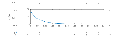
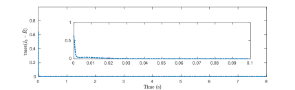
Figure 1: Estimation errors on the position direction and orientation.

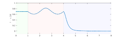
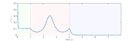
Figure 2: Estimation error on the position range and the Lyapunov function value during motion phases: (a) in green, (b) in red and (c) in blue.

7 Conclusions

We presented an equivariant observer design to estimate relative pose using epipolar geometry and velocity measurements. The approach is based on a novel polar symmetry employed to parametrize 3D pose, efficiently decoupling the bearing and range components and naturally aligning with the scale-invariance of the epipolar constraint. Comprehensive observability and stability analyses were carried out in support of the proposed observer establishing an explicit persistence of excitation condition to ensure the uniform observability of the range component. The provided simulations validate the theoretical results and illustrate the performance of the proposed approach.

Appendix A Proofs

Proof of Proposition 1.

The identity property $\phi\left((I_{3},I_{3},1),(R,x)\right)=(R,x)$ is straightfoward to verify for any $(R,x)\in\mathcal{M}$. Let $(R,x)\in\mathcal{M}$ and $(S_{1},Q_{1},r_{1}),(S_{2},Q_{2},r_{2})\in\mathbf{G}$ be arbitrary. Then

$$\phi\left((S_{2},Q_{2},r_{2}),\phi\left((S_{1},Q_{1},r_{1}),(R,x)\right)\right) =\phi\left((S_{2},Q_{2},r_{2}),\left(Q_{1}^{\top}RS_{1},r_{1}^{-1}Q_{1}^{\top}x\right)\right),$$

$$=\left(Q_{2}^{\top}Q_{1}^{\top}RS_{1}S_{2},r_{2}^{-1}Q_{2}^{\top}\left(r_{1}^{-1}Q_{1}^{\top}x\right)\right),$$

$$=\left((Q_{1}Q_{2})^{\top}RS_{1}S_{2},(r_{1}r_{2})^{-1}(Q_{1}Q_{2})^{\top}x\right),$$

$$=\phi\left((S_{1}S_{2},Q_{1}Q_{2},r_{1}r_{2}),(R,x)\right),$$

$$=\phi\left((S_{1},Q_{1},r_{1})(S_{2},Q_{2},r_{2}),(R,x)\right),$$

so it satisfies compatibility and it follows that $\phi$ is a right action. The transitivity follows from the property that $\phi((S,Q,r),(I_{3},x_{0}))=(S^{\top}Q,r^{-1}Q^{\top}x_{0})$ and hence it is straightforward to see any point in $\mathcal{M}$ can be reached from $(I_{3},x_{0})$ by suitable construction of an element of $\mathbf{G}$. This completes the proof. ∎

Proof of Proposition 2.

The identity property $\psi\left((I_{3},I_{3},1),(\Omega,v)\right)=(\Omega,v)$ is straightfoward to verify for any $(\Omega,v)\in\mathbb{V}$. Let $(\Omega,v)\in\mathbb{V}$ and $(S_{1},Q_{1},r_{1}),(S_{2},Q_{2},r_{2})\in\mathbf{G}$ be arbitrary. Then

$$\psi\left((S_{2},Q_{2},r_{2}),\psi\left((S_{1},Q_{1},r_{1}),(\Omega,v)\right)\right) =\psi\left((S_{2},Q_{2},r_{2}),\left(S_{1}^{\top}\Omega,r_{1}^{-1}S_{1}^{\top}v\right)\right),$$

$$=\left(S_{2}^{\top}S_{1}^{\top}\Omega,r_{2}^{-1}S_{2}^{\top}\left(r_{1}^{-1}S_{1}^{\top}v\right)\right),$$

$$=\left((S_{1}S_{2})^{\top}\Omega,(r_{1}r_{2})^{-1}(S_{1}S_{2})^{\top}v\right),$$

$$=\psi\left((S_{1}S_{2},Q_{1}Q_{2},r_{1}r_{2}),(\Omega,v)\right),$$

$$=\psi\left((S_{1},Q_{1},r_{1})(S_{2},Q_{2},r_{2}),(\Omega,v)\right),$$

so it satisfies compatibility. This demonstrates that $\psi$ is a right action as required. ∎

Proof of Proposition 3.

Let $(S,Q,r)\in\mathbf{G}$, $(R,x)\in\mathcal{M}$ and $(\Omega,v)\in\mathbb{V}$ be arbitrary. Note that $\phi$ is linear in $R$ and $x$, so $\mathrm{D}\phi_{X}$ acts on $f(\xi,u)$ the same way that $\phi_{X}$ acts on $\xi$. Therefore, one has

$$\mathrm{D}\phi_{(S,Q,r)}f\left((R,x),(\Omega,v)\right) =\mathrm{D}\phi_{X}\left(R\Omega^{\times},Rv\right),$$

$$=\left(Q^{\top}R\Omega^{\times}S,r^{-1}Q^{\top}Rv\right),$$

$$=\left(Q^{\top}RSS^{\top}\Omega^{\times}S,r^{-1}Q^{\top}RSS^{\top}v\right),$$

$$=\left((Q^{\top}RS)(S^{\top}\Omega)^{\times},(Q^{\top}RS)\left(r^{-1}S^{\top}v\right)\right),$$

$$=f\left(\phi((S,Q,r),(R,x)),\psi((S,Q,r),(\Omega,v))\right).$$

This proves that the kinematics (6) are equivariant under the symmetries $\phi$ and $\psi$. ∎

Proof of Proposition 4.

It is straightforward to verify that $\theta$ is a right action of $\mathbf{G}$ on $\mathcal{P}$. To show the invariance of $h$, it is sufficient to show that the the component functions $h^{i}$ are invariant under the actions $\phi$ and $\theta$. Let $(S,Q,r)\in\mathbf{G}$, $(R,t)\in\mathcal{M}$ and $(\mathring{p}_{i},p_{i})\in\mathcal{P}_{i}$ be arbitrary. Then,

$$h^{i}\left(\phi\left((S,Q,r),(R,x)\right);\theta\left((S,Q,r),(\mathring{p}_{i},p_{i})\right)\right) =h^{i}\left(\left(Q^{\top}RS,r^{-1}Q^{\top}x\right);\left(Q^{\top}\mathring{p}_{i},S^{\top}p_{i}\right)\right),$$

$$=\left(Q^{\top}\mathring{p}_{i}\right)^{\top}\frac{\left(r^{-1}Q^{\top}x\right)^{\times}}{|r^{-1}Q^{\top}x|}(Q^{\top}RS)(S^{\top}p_{i}),$$

$$=\mathring{p}_{i}^{\top}QQ^{\top}x_{d}^{\times}QQ^{\top}RSS^{\top}p_{i},$$

$$=\mathring{p}_{i}^{\top}x_{d}^{\times}Rp_{i}=h^{i}((R,x);(\mathring{p}_{i},p_{i})).$$

It follows that

$$h\left(\phi\left((S,Q,r),(R,x)\right);\theta\left((S,Q,r),\mathbf{p}\right)\right)$$

$$=\left(h^{1}\left(\phi\left((S,Q,r),(R,x)\right);\theta\left((S,Q,r),\mathbf{p}_{1}\right)\right),\dots,h^{m}\left(\phi\left((S,Q,r),(R,x)\right);\theta\left((S,Q,r),\mathbf{p}_{m}\right)\right)\right)$$

$$=\left(h^{1}\left((R,x);\mathbf{p}_{1}\right),\dots,h^{m}\left((R,x);\mathbf{p}_{m}\right)\right)$$

$$=h\left((R,x);\mathbf{p}\right).$$

This shows that, indeed, $h$ is invariant under the actions $\phi$ and $\theta$. ∎

Proof of Proposition 5.

Recall that $\phi((S,Q,r),(R,x)=\left(Q^{\top}RS,r^{-1}Q^{\top}x\right)$. To find $\mathrm{D}_{(S,Q,r)|(I_{3},I_{3},1)}\phi_{\xi}$ first choose $s\in\mathfrak{so}(3)$, $q\in\mathfrak{so}(3)$ and $b\in\mathfrak{mr}(1)$, and then evaluate $\phi$ applied to $S=e^{ts}$, $Q=e^{tq}$ and $r=e^{tb}$:

$$\mathrm{D}_{(S,Q,r)|(I_{3},I_{3},1)}\phi_{\xi}(s,q,b) =\frac{\mathrm{d}}{\mathrm{d}t}\phi((e^{ta},e^{tq},e^{tb}),(R,x))\mid_{t=0},$$

$$=\frac{\mathrm{d}}{\mathrm{d}t}(e^{-tq}Re^{ts},e^{-tb}e^{-tq}x)\mid_{t=0},$$

$$=(-qR+Rs,-(bI_{3}+q)x),$$

and so

$$\mathrm{D}_{X|{\text{id}}}\phi_{\xi}[\Lambda(\xi,u)] =\left(\left(\frac{x^{\times}Rv}{|x|^{2}}\right)^{\times}R+R\left(\Omega-\frac{(R^{\top}x)^{\times}v}{|x|^{2}}\right)^{\times},\frac{1}{|x|^{2}}\left((x^{\top}Rv)I_{3}+(x^{\times}Rv)^{\times}\right)x\right),$$

$$=\left(RR^{\top}\left(\frac{x^{\times}Rv}{|x|^{2}}\right)^{\times}R+R\left(\Omega-\frac{(R^{\top}x)^{\times}v}{|x|^{2}}\right)^{\times},\frac{1}{|x|^{2}}\left(\langle x,Rv\rangle I_{3}+x^{\times}(Rv)^{\times}-(Rv)^{\times}x^{\times}\right)x\right),$$

$$=\left(R\left(\frac{R^{\top}x^{\times}Rv}{|x|^{2}}+\Omega-\frac{(R^{\top}x)^{\times}v}{|x|^{2}}\right)^{\times},\frac{1}{|x|^{2}}\left(xx^{\top}Rv-x^{\times}x^{\times}Rv\right)\right),$$

$$=\left(R\left(\frac{(R^{\top}x)^{\times}v}{|x|^{2}}+\Omega-\frac{(R^{\top}x)^{\times}v}{|x|^{2}}\right)^{\times},\left(\frac{xx^{\top}}{|x|^{2}}-\frac{x^{\times}x^{\times}}{|x|^{2}}\right)Rv\right),$$

$$=\left(R\Omega^{\times},\left(\frac{xx^{\top}}{|x|^{2}}+\Pi_{x}\right)Rv\right),$$

$$=\left(R\Omega^{\times},Rv\right)=f\left(\xi,u\right).$$

As required. Now to show that the lift $\Lambda$ is equivariant

$$\mathrm{Ad}_{X^{-1}}(\Lambda(\xi,u))$$

$$=\mathrm{Ad}_{X^{-1}}\left(\left(\Omega-\frac{(R^{\top}x)^{\times}v}{|x|^{2}}\right)^{\times},-\frac{\left(x^{\times}Rv\right)^{\times}}{|x|^{2}},-\frac{x^{\top}Rv}{|x|^{2}}\right),$$

$$=\left(S^{\top}\left(\Omega-\frac{(R^{\top}x)^{\times}v}{|x|^{2}}\right)^{\times}S,-Q^{\top}\left(\frac{x^{\times}Rv}{|x|^{2}}\right)^{\times}Q,\frac{(Q^{\top}x/r)^{\top}(Q^{\top}RS)(S^{\top}v/r)}{|Q^{\top}x/r|^{2}}\right),$$

$$=\left(\left(S^{\top}\Omega-\frac{S^{\top}R^{\top}x^{\times}Rv}{|x|^{2}}\right)^{\times},-\left(\frac{Q^{\top}x^{\times}Rv}{|x|^{2}}\right)^{\times},\frac{(Q^{\top}x/r)^{\top}(Q^{\top}RS)(S^{\top}v/r)}{|Q^{\top}x/r|^{2}}\right),$$

$$=\left(\left(S^{\top}\Omega-\frac{S^{\top}R^{\top}QQ^{\top}x^{\times}QQ^{\top}RSS^{\top}v}{|x|^{2}}\right)^{\times},-\left(\frac{Q^{\top}x^{\times}QQ^{\top}RSS^{\top}v}{|x|^{2}}\right)^{\times},\frac{(Q^{\top}x/r)^{\top}(Q^{\top}RS)(S^{\top}v/r)}{|Q^{\top}x/r|^{2}}\right),$$

$$=\left(\left(S^{\top}\Omega-\frac{(Q^{\top}RS)^{\top}(Q^{\top}x/r)^{\times}(Q^{\top}RS)(S^{\top}v/r)}{|Q^{\top}x/r|^{2}}\right)^{\times},-\left(\frac{(Q^{\top}x/r)^{\times}(Q^{\top}RS)(S^{\top}v/r)}{|Q^{\top}x/r|^{2}}\right)^{\times},\frac{(Q^{\top}x/r)^{\top}(Q^{\top}RS)(S^{\top}v/r)}{|Q^{\top}x/r|^{2}}\right),$$

$$=f\left(\left(Q^{\top}RS,r^{-1}Q^{\top}x\right),\left(S^{\top}\Omega,r^{-1}S^{\top}v\right)\right),$$

$$=f\left(\phi\left((S,Q,r),(R,t)\right),\psi\left((S,Q,r),(\Omega,v)\right)\right).$$

As required. ∎

References

• Longuet-Higgins [1981] H Christopher Longuet-Higgins. A computer algorithm for reconstructing a scene from two projections. Nature, 293(5828):133–135, 1981.
• Hartley and Zisserman [2003] Richard Hartley and Andrew Zisserman. Multiple view geometry in computer vision. Cambridge university press, 2003.
• Nistér [2004] David Nistér. An efficient solution to the five-point relative pose problem. IEEE transactions on pattern analysis and machine intelligence, 26(6):756–770, 2004.
• Hartley [1997] Richard I Hartley. In defense of the eight-point algorithm. IEEE Transactions on pattern analysis and machine intelligence, 19(6):580–593, 1997.
• Ma et al. [2001] Yi Ma, Jana Košecká, and Shankar Sastry. Optimization criteria and geometric algorithms for motion and structure estimation. International Journal of Computer Vision, 44:219–249, 2001.
• Botterill et al. [2011] Tom Botterill, Steven Mills, and Richard Green. Refining essential matrix estimates from ransac. In Proceedings Image and Vision Computing New Zealand, pages 1–6, 2011.
• White and Beard [2020] Jacob H White and Randal W Beard. An iterative pose estimation algorithm based on epipolar geometry with application to multi-target tracking. IEEE/CAA Journal of Automatica Sinica, 7(4):942–953, 2020.
• Hua et al. [2020] Minh-Duc Hua, Simone De Marco, Tarek Hamel, and Randal W Beard. Relative pose estimation from bearing measurements of three unknown source points. In 2020 59th IEEE Conference on Decision and Control (CDC), pages 4176–4181. IEEE, 2020.
• Julier and LaViola [2007] Simon J Julier and Joseph J LaViola. On kalman filtering with nonlinear equality constraints. IEEE Transactions on Signal Processing, 55(6):2774–2784, 2007.
• Gintrand et al. [2022] Pierre Gintrand, Minh-Duc Hua, Tarek Hamel, and Guillaume Varra. On the uniform observability of the relative pose estimation problem using bearing measurements and epipolar constraints. In 2022 IEEE 61st Conference on Decision and Control (CDC), pages 3468–3474. IEEE, 2022.
• van Goor et al. [2019] Pieter van Goor, Robert Mahony, Tarek Hamel, and Jochen Trumpf. A geometric observer design for visual localisation and mapping. In 2019 IEEE 58th Conference on Decision and Control (CDC), pages 2543–2549. IEEE, 2019.
• van Goor et al. [2020] Pieter van Goor, Tarek Hamel, and Robert Mahony. Equivariant filter (eqf): A general filter design for systems on homogeneous spaces. In 2020 59th IEEE Conference on Decision and Control (CDC), pages 5401–5408. IEEE, 2020.
• van Goor et al. [2023] Pieter van Goor, Tarek Hamel, and Robert Mahony. Equivariant filter (eqf). IEEE Transactions on Automatic Control, 68(6):3501–3512, 2023. doi:10.1109/TAC.2022.3194094.
• Morin et al. [2017] Pascal Morin, Alexandre Eudes, and Glauco Scandaroli. Uniform observability of linear time-varying systems and application to robotics problems. In Geometric Science of Information: Third International Conference, GSI 2017, Paris, France, November 7-9, 2017, Proceedings 3, pages 336–344. Springer, 2017.
• Mahony et al. [2022] Robert Mahony, Pieter van Goor, and Tarek Hamel. Observer design for nonlinear systems with equivariance. Annual Review of Control, Robotics, and Autonomous Systems, 5:221–252, 2022.
• van Goor and Mahony [2023] Pieter van Goor and Robert Mahony. Eqvio: An equivariant filter for visual-inertial odometry. IEEE Transactions on Robotics, 2023.
• Hamel and Samson [2017] Tarek Hamel and Claude Samson. Riccati observers for the nonstationary pnp problem. IEEE Transactions on Automatic Control, 63(3):726–741, 2017.