On the ergodicity breaking in well-behaved Generalized Langevin Equations

Abstract

The phenomenon of ergodicity breaking of stochastic dynamics governed by Generalized Langevin Equations (GLE) in the presence of well-behaved exponentially decaying dissipative memory kernels, recently investigated by many authors (Phys. Rev. E 83 062102 2011; Phys. Rev. E 98 062140 2018; Eur. Phys. J. B 93 184 2020), finds, in the dynamic theory of GLE, its simple and natural explanation, related to the concept of dissipative stability. It is shown that the occurrence of ergodicity breakdown for well-behaved dissipative kernels falls, in general, ouside the region of stochastic realizability, and therefore it cannot be observed in physical systems.

I Introduction

Since the work by Kubo kubo1 ; kubo2 , the use of Generalized Langevin Equations (GLE) to describe physical systems driven by thermal fluctuations, their equilibrium properties and their response to external perturbations, has become a standard procedure that applies in the linear regime from Brownian dynamics to dielectric response, from electrochemical processes to magnetization phenomena. If $A(t)$ is the physical observable, the GLE describing its linear dynamics at thermal equilibrium takes the form

$$\frac{dA(t)}{dt}=-\int_{0}^{t}M(t-\tau)\,A(\tau)\,d\tau+R(t)$$ (1)

where $M(t)$ is a memory kernel accounting for dissipation, and $R(t)$ is the stochastic forcing associated with the thermal fluctuations. In order to focus the idea on a concrete physical problem, consider the case where $A(t)=m\,v(t)$ is the momentum of a (spherical) particle of mass $m$ in a fluid medium, so that eq. (1) can be rewritten in terms of the particle velocity $v(t)$ as

$$m\,\frac{dv(t)}{dt}=-\int_{0}^{t}h(t-\tau)\,v(\tau)\,d\tau+R(t)$$ (2)

where $h(t)=m\,M(t)$, and eq. (2) is coupled with the kinematic equation

$$\frac{dx(t)}{dt}=v(t)$$ (3)

As regards $R(t)$, the classical assumption in GLE theory is that the thermal fluctuations are independent of the velocity, and this can be expressed by the Langevin condition langevin

$$\langle R(t)\,v(0)\,\rangle_{\rm eq}=0\,,\qquad t\geq 0$$ (4)

where $\langle\cdot\rangle_{\rm eq}$ indicates the expected value with respect to the probability measure of the thermal fluctuations at equilibrium (at constant temperature $T$).

The kernel $h(t)$ accounts for the dissipative nature of the interactions that, combined with the fluctuating contribution $R(t)$, determines the relaxation towards equilibrium. In the case of the equation of motion for a Brownian particle eq. (2), the kernel $h(t)$ represents the dynamic friction factor procopio2 , proportional to the dynamic viscosity of the medium rheol1 ; rheol2 . For a Newtonian fluid in the Stokes regime $h(t)$ is impulsive and this corresponds to the classical Einstein-Langevin description of Brownian motion. For more complex fluids, viscoelastic effects becomes important at the time-scales of interest (both in theory and in the applications) franosch and $h(t)$ becomes a continuous function of time.

The basic condition in the classical Kubo theory to be imposed on $h(t)$ is that the long-term friction coefficient $\eta_{\infty}$,

$$\eta_{\infty}=\int_{0}^{\infty}h(t)\,dt\geq 0$$ (5)

is positive kubo1 ; kubo2 . More precisely, three cases may occur: (i) if $\eta_{\infty}>0$ and bounded, then particle dynamics is in the long-term diffusive, i.e. $\langle x^{2}(t)\rangle\simeq 2\,D\,t$, where the diffusivity $D$ is related to $\eta_{\infty}$ by the global fluctuation-dissipation relation

$$D\,\eta_{\infty}=k_{B}\,T$$ (6)

where $k_{B}$ is the Boltzmann constant; (ii) $\eta_{\infty}=\infty$, and in this case anomalous subdiffusive behavior may occur; (iii) $\eta_{\infty}=0$, corresponding to the absence of any dissipation, and this gives rise either to anomalous superdiffusive scaling or the breaking or ergodicity goychuk1 ; goychuk2 ; goychuk3 .

This picture has been questioned by a series of interesting contributions bao1 ; bao2 ; bao3 ; plyukhin1 ; plyukhin2 that showed that, even if $\eta_{\infty}$ is positive and finite and the kernel $h(t)$ possesses a regular exponentially decaying behavior with $t$, (i.e., $|h(t)|\leq C\,e^{-k\,t}$, for some $C>0$ and $k>0$), ergodicity breaking may occur, associated with a non-vanishing long-term scaling of the velocity autocorrelation function $C_{vv}(t)=\langle v(t)\,v(0)\rangle_{\rm eq}$. The latter property implies that there exists a monotonically increasing and diverging sequence of time instants $\{t_{n}\}_{n=1}^{\infty}$, $t_{n}<t_{n+1}$, $\lim_{n\rightarrow\infty}t_{n}=\infty$, and a constant $K>0$ such that $|C_{vv}(t_{n})|\geq K$. We use the diction of “well-behaved” dissipative kernels for $h(t)$’s possessing the following properties: (i) $\eta_{\infty}>0$; (ii) $h(t)$ is an exponentially decaying function of $t$ for large times; (iii) $h(t)\geq 0$. Condition (iii) usually emerges as a physical empirical constraint (i.e. dictated by the phenomenological experience) on the viscoelastic response of complex fluids. The model considered in bao3 fulfils conditions (i) and (ii) but not (iii). Nevertheless it is also considered below for its mathematical interest, as a non-hydrodynamic model of relaxation.

In point of fact, the results discussed in bao1 ; bao2 ; bao3 ; plyukhin1 ; plyukhin2 on the ergodicity breaking in well-behaved dissipative systems can be viewed as a particular case of the dynamic theory developed in gpp for GLE, in which it is shows that eq. (5) is by no mean a sufficient condition to establish the relaxation towards a stable equilibrium behavior and the validity of the global Stokes-Einstein relation eq. (6), as intrinsic instabilities in the internal memory dynamics governed by the kernel $h(t)$ may occur, leading to a diverging behavior in time of the velocity autocorrelation function. More precisely, the ergodicity breaking observed in bao1 ; bao2 ; bao3 ; plyukhin1 ; plyukhin2 corresponds to operating conditions lying at the boundary of the region of (dissipative) stability as defined in gpp . Following the analysis developed in gpp , in order to observe these phenomena from the dynamic evolution of physical systems described via GLE, the further condition of stochastic realizability should be met. As will be thoroughly addressed below, the phenomena of ergodicity breaking reported in bao1 ; bao2 ; bao3 ; plyukhin1 ; plyukhin2 cannot occur in general due to the lack of stochastic realizability gpp . The aim of this brief report is to address in detail these issues in full clarity, by analyzing two benchmarking examples: kernels $h(t)$ possessing two real-valued relaxation exponents, and the model addressed by Plyukhin in bao3 .

II Dynamic GLE theory

To begin with, let us review the main results developed in gpp that are functional to the present analysis. Without loss of generality, asume that $h(t)$ can be expressed as a series of exponentially decaying functions of times (modes) plus an impulsive contribution

$$h(t)=\sum_{k=1}^{N}h_{k}\,e^{-\lambda_{k}\,t}+H_{0}\,\delta(t)$$ (7)

where $\lambda_{k}\in{\mathbb{C}}$, $k=1,\dots,N$ are complex-valued exponents, and consequently $h_{k}\in{\mathbb{C}}$, such that the sum entering eq. (8) is real-valued for any $t\geq 0$, and $H_{0}>0$. Moreover, let us assume that $\mbox{Re}[\lambda_{k}]>0$, $k=1,\dots,N$, so that $h(t)$ decays exponentially with $t$, and that

$$\eta_{\infty}=H_{0}+\sum_{k=1}^{N}\frac{h_{k}}{\lambda_{k}}>0$$ (8)

and bounded, where obviously the sum in eq. (8) is real-valued.

Eq. (7) essentially corresponds to the existence of a Markovian embedding for the GLE. It has been argumented in gpp that this representation, considering the limit for $N\rightarrow\infty$, constitutes the most general structure for the linear response of a physical system that is local in time. The only exception to this claim occurs in some particular cases where the particle interacts with a field, e.g. the hydrodynamic velocity field of a continuous liquid phase, determining in the Newtonian case the occurrence of a fluid-inertial memory contribution to $h(t)$ proportional to $1/\sqrt{t}$ (the Basset force) landau . But even this case reduces to eq. (7) (with a countable set of modes) if the finite propagation velocity of the shear stresses is accounted for procopio2 . In any case, a further discussion on this important conceptual point is completely immaterial in the present analysis as all the examples considered in bao1 ; bao2 ; bao3 ; plyukhin1 ; plyukhin2 refer to the modal representaton eq. (7) with $N$ finite and small.

Given eq. (7), the GLE can be represented as

$$m\,\frac{dv(t)}{dt} = -\sum_{k=1}^{N}\widetilde{h}_{k}\,z_{k}(t)-H_{0}\,v(t)+\sqrt{2}\,\beta_{0,0}\,\xi_{0}(t)+\sqrt{2}\,\sum_{k=1}^{N}\beta_{0,k}\,\xi_{k}(t)$$

$$\frac{dz_{k}(t)}{dt} = -\lambda_{k}\,z_{k}(t)+b_{k}\,v(t)+\sqrt{2}\,\beta_{k,0}\,\xi_{0}(t)+\sqrt{2}\,\sum_{h=1}^{N}\beta_{k,h}\,\xi_{k}(t)$$ (9)

where $\xi_{0}(t)$, $\xi_{k}(t)$, $k=1,\dots,N$ are independent white-noise processes vankampen , $\langle\xi_{h}(t)\,\xi_{k}(t^{\prime})\rangle=\delta_{h,k}\,\delta(t-t^{\prime})$, $h,k=0,\dots,N$, $t,\,t^{\prime}\in{\mathbb{R}}$, e.g. distributional derivatives of independent Wiener processes (corresponding to the classical approach adopted in statistical physics and followed also in the present work), and

$$b_{k}\,\widetilde{h}_{k}=h_{k}\,,\qquad k=1,\dots,N$$ (10)

The coefficients $\beta_{h,k}$, $h,k=0,\dots,N$, modulating the intensity of the stochastic fluctuations, are to be determined from the Langevin condition eq. (4), indicating that the thermal fluctuations at any time instant $t$ are independent of the previous history of particle velocity. This leads automatically to the equations for the velocity autocorrelation function $C_{vv}(t)$

$$m\,\frac{dC_{vv}(t)}{dt} = -\sum_{k=1}^{N}\widetilde{h}_{k}\,C_{z_{k}v}(t)$$

$$\frac{dC_{z_{k}v}(t)}{dt} = -\lambda_{k}\,C_{z_{k}v}(t)+b_{k}\,C_{vv}(t)\,,\qquad k=1,\dots,N$$ (11)

where $C_{z_{k}v}(t)=\langle z_{k}(t)\,v(0)\rangle_{\rm eq}$, $k=1,\dots,N$, equipped with the initial conditions

$$C_{vv}(0)=\langle v^{2}\rangle_{\rm eq}=\frac{k_{B}\,T}{m}\,,\qquad C_{z_{k}v}(0)=0\,\quad k=1,\dots,N$$ (12)

Eqs. (11)-(12) are usually referred to as the fluctuation-dissipation relation (theorem, in the Kubo description kubo1 ; kubo2 ) of the first kind.

The structure of the stochastic perturbations entering eq. (9), and its white-noise nature represents the most general setting consistent with the Langevin conditions eq. (4). Henceforth, let us consider the nondimensional formulation of the equations of motion, rescaling the velocity to its equilibrium intensity, and time with respect to a characteristic dissipation time. In practice, and without loss of generality, this means that we can set $m=1$, $\langle v^{2}\rangle_{\rm eq}=1$, while the remaining coefficients $\widetilde{h}_{k}$, $H_{0}$, $\lambda_{k}$, $b_{k}$ are dimensionless. Setting ${\bf y}=(v,z_{1},\dots,z_{N})$, $\bm{\xi}=(\xi_{0},\xi_{1},\dots,\xi_{N})$ eq. (9) can be compactly expressed as

$$\frac{d{\bf y}(t)}{dt}={\bf A}\,{\bf y}(t)+\sqrt{2}\,\bm{\beta}\,\bm{\xi}(t)$$ (13)

where the coefficient matrix ${\bf A}$ governing the internal mode dynamics is given by

$${\bf A}=\left(\begin{array}[]{ccccc}-H_{0}&-\widetilde{h}_{1}&\dots&\dots&-\widetilde{h}_{N}\\ b_{1}&-\lambda_{1}&0&\dots&0\\ b_{2}&0&-\lambda_{2}&\dots&0\\ \dots&\dots&\dots&\dots&\dots\\ b_{N}&0&0&\dots&-\lambda_{N}\end{array}\right)$$ (14)

$\bm{\beta}=(\beta_{h,k})_{h,k=0}^{N}$, and $\bm{\beta}\,\bm{\xi}(t)$ corresponds to the row-by-column matrix multiplication of vector $\bm{\xi}(t)$ by the matrix $\bm{\beta}$.

In order to enforce fluctuation-dissipation relations, two basic properties should be fulfilled gpp , namely

• dissipative stability, corresponding to the fact that all the eigenvalues $\nu_{k}$, $k=0,\dots,N$ of the coefficient matrix ${\bf A}$ possess negative real part;

• stochastic realizability, corresponding to the fact that there exists a matrix $\bm{\beta}$ of stochastic intensities such as, given the stochastic process eq. (10), the fluctuation-dissipation relation of the first kind, i.e., eqs. (11)-(12) for $C_{vv}(t)$, is fulfilled.

If the system is dissipatively unstable, i.e., if there exists at least one eigenvalue of ${\bf A}$, say $\nu_{k^{*}}$, with $\mbox{Re}[\nu_{k}^{*}]>0$, no equilibrium conditions can be set. As a consequence, no diffusive dynamics exists and the Stokes-Einstein relations cannot be applied. But even if a GLE is dissipatively stable, this does not necessarily implies that the thermal fluctuations could be expressed in the form of a stochastic process $R(t)$ entering eq. (2) and such that it fulfils the Langevin condition eq. (4). In order to ensure it, the requirement of stochastic realizability should be further enforced.

In the light of the phenomenology envisaged by the ergodicity breaking addressed in bao1 ; bao2 ; bao3 ; plyukhin1 ; plyukhin2 , the dynamic theory of GLE simply indicates that this occurs at the boundary separating the region of parameters for which the GLE is dissipatively stable from the instability region.

In the remainder we consider two prototypical examples, showing in general that the condition of stochastic realizability is more stringent than dissipative stability, and consequently, in most of the situations, a stochastic GLE with well-behaved kernel providing ergodicity breaking cannot be defined within the realm of the actual theory of GLE, in the meaning that there is no stochastic process $R(t)$ fulfilling the Langevin condition eq. (4), such that the resulting GLE eq. (2) satisfy the fluctuation-dissipation relation of the first kind.

III Two real-mode dynamics

To begin with, consider the case of two real modes, i.e.,

$$h(t)=h_{1}\,e^{-\lambda_{1}\,t}+h_{2}\,e^{-\lambda_{2}\,t}$$ (15)

setting $h_{1}=1$, $\lambda_{1},\lambda_{2}>0$, $\lambda_{1}<\lambda_{2}$. The case of real modes occurs in the study of particle motion in linear viscoelastic fluids, where the values of the coefficients/exponents, $h_{k}$ and $\lambda_{k}$, respectively, can be determined from the analysis of rheological experiments rheol1 ; rheol2 . In the present context, the case of major interest is where $h_{2}=-\alpha<0$, as the system is both dissipatively stable and stochastically realizable for any non-negative values of $h_{k}$. From eq. (15), setting without loss of generality, all the $b_{k}^{\prime}s$ equal to 1 in eq. (9), the expression of the coefficient matrix ${\bf A}$ becomes

$${\bf A}=\left(\begin{array}[]{ccc}0&-h_{1}&\alpha\\ 1&-\lambda_{1}&0\\ 1&0&-\lambda_{2}\end{array}\right)$$ (16)

and $\alpha$ is used as a parameter controlling the qualitative properties of the GLE. Following the dynamical theory of GLE gpp , three different characteristic values of $\alpha$ can be defined. The first one is the threshold $\alpha^{*}$, corresponding to the situation where $\eta_{\infty}|_{\alpha=\alpha^{*}}=0$, i.e.,

$$\alpha^{*}=\frac{\lambda_{2}\,h_{1}}{\lambda_{1}}$$ (17)

For $\alpha<\alpha^{*}$ $\eta_{\infty}>0$, while the global dissipative properties are lost for $\alpha>\alpha^{*}$ and in this region the fluid acts as an actively destabilizing environment for particle dynamics. The second critical value $\alpha_{\rm ds}$ determines the boundary of the region of dissipative stability, as for $\alpha>\alpha_{\rm ds}$ the system is unstable. In the present case, $\alpha_{\rm ds}$ can be calculated in an easy way, observing that the matrix ${\bf A}$ possesses one real eigenvalue and a couple of complex conjugate eigenvalues, and that instability originates from the complex-conjugate branch (this follows from the direct spectral analysis of the system). Letting Tr, $M_{2}$ and Det be the three algebraic invariants of ${\bf A}$,

$$\mbox{Tr}=-(\lambda_{1}+\lambda_{2})\,,\quad M_{2}=\lambda_{1}\,\lambda_{2}+h_{1}+h_{2}\,,\quad\mbox{Det}=-(h_{1}\,\lambda_{2}+h_{2}\,\lambda_{1})$$ (18)

the critical value $\alpha_{\rm ds}$ of $\alpha$ (cfr. $h_{2}=-\alpha$) occurs when $\mbox{Det}=\mbox{Tr}\,M_{2}$, corresponding to the condition where the complex eigenvalue branch admits vanishing real part. This leads to the expression for $\alpha_{\rm ds}$,

$$\alpha_{\rm ds}=-\frac{1}{\lambda_{2}}\,\left[h_{1}\,\lambda_{2}-(\lambda_{1}+\lambda_{2})(\lambda_{1}\,\lambda_{2}+h_{1})\right]$$ (19)

Finally, the last critical value corresponds to $\alpha_{\rm sr}$, determining the upper value of $\alpha$ at which the GLE is stochastically realizable. By considering the general structure of the stochastic perturbation in eq. (9) (with $H_{0}=0$ and $m=1$), the most general stochastic realization of the system takes the form

$$\frac{dv(t)}{dt} = -h_{1}\,z_{1}(t)+\alpha\,z_{2}(t)$$

$$\frac{dz_{1}(t)}{dt} = -\lambda_{1}\,z_{1}(t)+v(t)+\sqrt{2}\left[\beta_{1,1}\,\xi_{1}(t)+\beta_{1,2}\,\xi_{2}(t)\right]$$ (20)

$$\frac{dz_{2}(t)}{dt} = -\lambda_{2}\,z_{2}(t)+v(t)+\sqrt{2}\left[\beta_{2,1}\,\xi_{1}(t)+\beta_{2,2}\,\xi_{2}(t)\right]$$

Observe that no direct coupling between $v(t)$ and a stochastic forcing may occur, since in present case no impulsive friction is present, and a direct stochastic forcing acting on $v(t)$ would determine the unbounded divergence of the velocity variance in time. The Fokker-Planck equation for the probability density $p(v,z_{1},z_{2},t)$ associated with eq. (20) reads

$$\frac{\partial p}{\partial t} = \left(h_{1}\,z_{1}-\alpha\,z_{2}\right)\,\frac{\partial p}{\partial v}-\frac{\partial\left[(-\lambda_{1}\,z_{1}+v)\,p\right]}{\partial z_{1}}-\frac{\partial\left[(-\lambda_{2}\,z_{2}+v)\,p\right]}{\partial z_{2}}$$ (21)

$$+ S_{1,1}\,\frac{\partial^{2}p}{\partial z_{1}^{2}}+2\,S_{1,2}\,\frac{\partial^{2}p}{\partial z_{1}\partial z_{2}}+S_{2,2}\,\frac{\partial^{2}p}{\partial z_{2}^{2}}$$

where ${\bf S}=(S_{i,j})_{i,j=1}^{2}$ is given by ${\bf S}=\bm{\beta}\,\bm{\beta}^{T}$, $\bm{\beta}=(\beta_{i,j})_{i,j=1}^{2}$ and “$T$” indicates the transpose. The GLE is stochastically realizable if there exists a $2\times 2$ positive definite matrix ${\bf S}$ entering eq. (21), such that the stationary (equilibrium) second-order moments satisfy the relations $\langle v^{2}\rangle_{\rm eq}=1$, $\langle z_{k}\,v\rangle_{\rm eq}=0$, $k=1,2$, that correspond to the fulfillment of the fluctuation-dissipation relation of the first kind. Second-order moments are considered as the first-order moment identically vanish at equilibrium. The details of this calculation can be found in gpp and therefore are not repeated here. The condition of positive definiteness of ${\bf S}$ implies that there exists values of $\zeta=S_{1,2}$ such that

$$\phi(\zeta)=-1+(\gamma_{2}-\gamma_{1})\,\zeta-\left(\gamma_{3}-\gamma_{1}\,\gamma_{2}\right)\,\zeta\geq 0$$ (22)

where

$$\gamma_{1}=-\frac{2\,h_{2}}{\lambda_{1}+\lambda_{2}}\,,\quad\gamma_{2}=\frac{2\,h_{1}}{\lambda_{1}+\lambda_{2}}\,,\quad\gamma_{3}=-\frac{h_{1}\,h_{2}}{\lambda_{1}\,\lambda_{2}}$$ (23)

Therefore, the critical value of $\alpha$, as regards stochastic realizability, corresponds to the situation when the local (and absolute) maximum $\phi^{*}$ of the function $\phi(\zeta)$ vanishes. As

$$\phi^{*}=\frac{(\gamma_{1}+\gamma_{2})^{2}-4\,\gamma_{3}}{4\,(\gamma_{3}-\gamma_{1}\,\gamma_{2})}$$ (24)

this implies $(\gamma_{1}+\gamma_{2})^{2}-4\,\gamma_{3}=0$, that solved with respect to $\alpha=\alpha_{\rm sr}$, provides

$$\alpha_{\rm sr}=-\left(\delta-\sqrt{\delta^{2}-h_{1}^{2}}\right)\,,\qquad\delta=h_{1}-\frac{h_{1}\,(\lambda_{1}+\lambda_{2})^{2}}{2\,\lambda_{1}\,\lambda_{2}}$$ (25)

Figure 1 depicts the behavior of $\alpha_{\rm sr}$, $\alpha_{\rm ds}$ and $\alpha^{*}$ vs $\lambda_{2}$ at three different values of $\lambda_{1}$ (with $h_{1}=1$). As can be observed, in all the situations

$$\alpha_{\rm sr}\leq\mbox{min}\{\alpha_{\rm ds},\alpha^{*}\}$$ (26)

and thus, in all the cases, $\alpha_{\rm sr}<\alpha_{\rm ds}$. This observation is relevant in the present analysis of the ergodicity breaking as it indicates that prior to observing a non ergodic behavior (corresponding to the conditions lying on the curves defining $\alpha_{\rm ds}$), the GLE becomes stochastically non realizable. Consequently, the ergodicity breaking cannot be observed from the stochastic dynamics of this system.

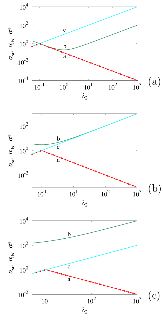
Figure 1: $\alpha_{\rm sr}$ (lines a and symbols $\bullet$), $\alpha_{\rm ds}$ (lines b) and $\alpha^{*}$ (lines c) vs $\lambda_{2}$, at three different values of $\lambda_{1}$ with $h_{1}=1$. Panel (a) refers to $\lambda_{1}=0.1$, panel (b) to $\lambda_{1}=1$, panel (c) to $\lambda_{1}=10$.

As an example consider the case $\lambda_{1}=0.1$, $\lambda_{2}=1.5$. In this case, $\alpha_{\rm sr}=2/30=0.0666..$, and $\alpha_{\rm ds}=34/15\simeq 0.2266..$. Figure 2 depicts the velocity autocorrelation function $C_{vv}(t)$ for a value of $\alpha=0.066$ below but close to $\alpha_{\rm sr}$. Symbols correspond to the stochastic simulations of the GLE, obtained by selecting a stochastic realization amongst all the possible equivalent ones at this value of $\alpha$ close to $\alpha_{\rm sr}$, considering a symmetric $\bm{\beta}$, and solving the matrix equation ${\bf S}=\bm{\beta}^{2}$.

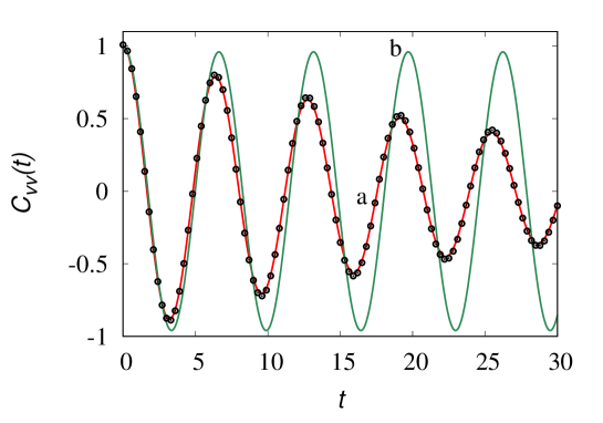
Figure 2: Velocity autocorrelation function $C_{vv}(t)$ vs $t$ for the two-mode system discussed in the main text at $\lambda_{1}=0.1$, $\lambda_{2}=1.5$, $\alpha=0.066<\alpha_{\rm sr}$. Symbols ($\circ$) represent the results of stochastic simulations, line (a) corresponds to the solution of eqs. (11)-(12) in the present case. Curve (b) corresponds to the autocorrelation function at $\alpha_{\rm ds}$.

Curve (b) in figure 2 represents the velocity autocorrelation function at $\alpha=\alpha_{\rm ds}$ i.e. at the condition of ergodicity breaking, when $C_{vv}(t)$ asymptotically oscillates without neither decaying to zero or diverging to infinity. It is worth observing that the phenomena of dynamic instability and stochastic irrealizability observed in this two-mode system correspond to extremely regular and well-behaved memory kernels, as depicted in figure 3.

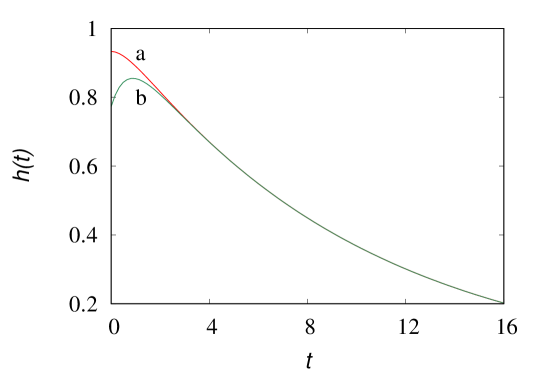
Figure 3: Memory kernels $h(t)$ vs $t$ for $\lambda_{1}=0.1$, $\lambda_{2}=1.5$ at the critical values. Line (a) refers to $\alpha=\alpha_{\rm sr}$, line (b) to $\alpha=\alpha_{\rm ds}$.

In the region between $\alpha_{\rm sr}$ and $\alpha_{\rm ds}$ the kernels attains positive values, and of course decay exponentially to zero for $t\rightarrow\infty$. Therefore, as addressed in gpp , the dynamic instabilities occurring for this class of GLE involve a much finer interaction mechanism amongst the internal modes accounting for the memory dynamics.

IV The Plyukhin dynamics

As a second case study, consider the model analyzed by Plyukhin bao3 . It corresponds to a memory kernel $h(t)$ of the form

$$h(t)=\delta(t)+\varepsilon\,e^{-\mu\,t}\,\sin(\omega\,t)$$ (27)

with $\mu=1/2$, $\omega=\sqrt{3}/2$. In bao3 , the critical value of $\varepsilon$ giving rise to the ergodicity breaking is $\varepsilon^{*}=2\,\sqrt{3}$. In the present analysis we consider $\varepsilon$ as a parameter. The stochastic realization of this system is expressed by

$$\frac{dv(t)}{dt} = -v(t)+\varepsilon\,z(t)+R_{v}(t)$$

$$\frac{dr(t)}{dt} = -\mu\,r(t)+\omega\,z(t)+v(t)+R_{r}(t)$$ (28)

$$\frac{dz(t)}{dt} = -\omega\,r(t)-\mu\,z(t)+R_{z}(t)$$

where $R_{k}(t)$, $\alpha=v,\,r,\,z$, are the stochastic forcings

$$R_{k}(t)=\sqrt{2}\,\left[\sum_{h=1}^{3}\beta_{k,h}\,\xi_{h}(t)\right]\,,\qquad k=v,\,r,\,z$$ (29)

and $\xi_{h}(t)$, $h=1,2,3$ are three independent white-noise processes (expressed also in this case as distributional derivatives of independent Wiener processes). Due to the presence of an impulsive contribution to friction, the stochastic forcing involves also a contribution acting directly on the velocity variable $v(t)$. The stability diagram associated with the coefficient matrix of this system vs the parameter $\varepsilon$ is represented in figure 4. Specifically, figure 4 depicts the largest real part $\nu_{\rm max}^{R}$ of the eigenvalues of the coefficient matrix ${\bf A}$,

$${\bf A}=\left(\begin{array}[]{ccc}-1&0&\varepsilon\\ 1&-\mu&\omega\\ 0&-\omega&-\mu\end{array}\right)$$ (30)

and the global friction coefficient $\eta_{\infty}=1+\varepsilon\,\omega/(\mu^{2}+\omega^{2})$.

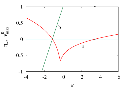
Figure 4: $\nu_{\rm max}^{R}$ (line a) and $\eta_{\infty}$ (line b) vs $\varepsilon$ for the Plyukhin model discussed in the main text. The symbol ($\bullet$), corresponding to the intesection of line (a) with the $x$-axis, marks the critical value $\varepsilon^{*}$.

As can be observed, the region of dissipative stability coincides with the interval $(\varepsilon_{\rm min},\varepsilon^{*})$, where $\varepsilon_{\rm min}$ is the value of $\varepsilon$ at which $\eta_{\infty}=0$, and $\varepsilon^{*}$ is the critical point associated with the ergodicity breaking analyzed in bao3 . It remains to determine the region of stochastic realizability. From eqs. (28)-(29), considering for the white-noise processes the distributional derivatives of independent Wiener processes, the associated Fokker-Planck equation for the density $p(v,r,z,t)$ reads

$$\frac{\partial p}{\partial t} = -\frac{\partial\left[(-v+\varepsilon\,z)\,p\right]}{\partial v}-\frac{\partial\left[(-\mu\,r+\omega\,z+v)\,p\right]}{\partial r}-\frac{\partial\left[(-\omega\,r-\mu\,z)\,p\right]}{\partial z}$$ (31)

$$+ S_{v,v}\,\frac{\partial^{2}p}{\partial v^{2}}+2S_{1,v}\,\frac{\partial^{2}p}{\partial v\partial r}+2S_{2,v}\,\frac{\partial^{2}p}{\partial v\partial z}+S_{1,1}\,\frac{\partial^{2}p}{\partial r^{2}}+2S_{1,2}\,\frac{\partial^{2}p}{\partial r\partial z}+S_{2,2}\,\frac{\partial^{2}p}{\partial z^{2}}$$

The system is stochastic realizable if there exists a positive definite symmetric matrix ${\bf S}$,

$${\bf S}=\left(\begin{array}[]{ccc}S_{v,v}&S_{1,v}&S_{2,v}\\ S_{1,v}&S_{1,1}&S_{1,2}\\ S_{2,v}&S_{1,2}&S_{2,2}\end{array}\right)$$ (32)

such that eq. (31) admits a stationary (equilibrium) density $p^{*}(v,r,z)$ possessing the following second-order moments $\langle v^{2}\rangle_{\rm eq}=1$, $\langle v\,r\rangle_{\rm eq}=\langle v\,z\rangle_{\rm eq}=0$, that ensure the correct behavior of the velocity autocorrelation function consistently with the fluctuation-dissipation relation of the first kind. It is convenient to introduce the following notation $m_{\alpha,\beta}(t)=\langle\alpha(t)\,\beta(t)\rangle$, $\alpha,\beta=v,r,z$, for the second-order moments. Observe that in this definition the expected value $\langle\cdot\rangle$ refers to generic non-equilibrium conditions i.e. to $p(v,r,z,t)$, and for this reason $m_{\alpha,\beta}(t)$ are functions of time. This should not be confused with the expected value $\langle\alpha\,\beta\rangle_{\rm eq}$ that refers to the equilibrium conditions (if they exist), i.e. to the invariant density $p^{*}(v,r,z)$ stationary solution of (31). It follows from eq. (31) the system of moment equations

$$\frac{dm_{v,v}}{dt} = -2\,m_{v,v}+2\,\varepsilon\,m_{v,z}+2\,S_{v,v}$$

$$\frac{dm_{v,r}}{dt} = -m_{v,r}+\varepsilon\,m_{r,z}-\mu\,m_{v,r}+\omega\,m_{v,z}+m_{v,v}+2\,S_{1,v}$$

$$\frac{dm_{v,z}}{dt} = -m_{v,z}+\varepsilon\,m_{z,z}-\omega\,m_{v,r}-\mu\,m_{v,z}+m_{v,v}+2\,S_{2,v}$$ (33)

$$\frac{dm_{r,r}}{dt} = 2\left(-\mu\,m_{r,r}+\omega\,m_{r,z}+m_{v,r}\right)+2\,S_{1,1}$$

$$\frac{dm_{z,z}}{dt} = 2\left(-\omega\,m_{r,z}-\mu\,m_{z,z}\right)+2\,S_{2,2}$$

$$\frac{dm_{r,z}}{dt} = \left(-\mu\,m_{r,z}+\omega_{z,z}+m_{v,z}\right)+\left(-\omega\,m_{r,r}-\mu\,m_{r,z}\right)+2\,S_{1,2}$$

Imposing the moment conditions, i.e. $m_{v,v}=1$, $m_{v,r}=m_{v,z}=0$ at equilibrium, we get from the moment equations at steady state

$$S_{v,v}=1\,,\quad m_{r,z}=-\frac{(1+2\,S_{1,v})}{\varepsilon}\,,\quad m_{z,z}=-\frac{2}{\varepsilon}\,S_{2,2}$$ (34)

that imply $S_{1,v}\in{\mathbb{R}}$, and $S_{2,v}<0$ if $\varepsilon>0$. Moreover

$$m_{r,r}=\frac{1}{\mu}\left[S_{1,1}-\frac{\omega}{\varepsilon}\,\left(1+2\,S_{1,v}\right)\right]$$ (35)

that implies that $S_{1,1}>S_{1,1}^{*}$, with $S_{1,1}^{*}=\omega\,\left(1+2\,S_{1,v}\right)/\varepsilon$. As regards the remaining entries of ${\bf S}$ we have,

$$S_{2,2} = \omega\,m_{r,z}+\mu\,m_{z,z}$$

$$S_{1,2} = \frac{1}{2}\left[2\,\mu\,m_{r,z}-\omega\,m_{z,z}+\omega\,m_{r,r}\right]$$ (36)

The analysis of stochastic realizability can be developed in terms of an extensive search by varying $S_{1,1}\in{\mathbb{R}}$, $S_{2,v}<0$ (since positive values of $\varepsilon$ are considered) and $S_{1,1}>S_{1,1}^{*}$, determining the remaining entries of the ${\bf S}$ matrix from the expressions reported above, and checking if the resulting ${\bf S}$ matrix is positive definite. In this way, the region of stochastic realizability for the Plyukhin model can be determined. Figure 5 depicts a projection of the region of stochastic realizability with respect to $S_{2,2}$ as a function of $\varepsilon$. For any value of $\varepsilon$ (in the region of stochastic realizability), there exists an interval $(S_{2,2}^{-},S_{2,2}^{+})$, such that for $S_{2,2}$ falling within this interval there are conditions (i.e. values of the other entries of ${\bf S}$) at which the system is stochastically realizable. Observe that from simulations the system is stochastically realizable up to a critical value $\varepsilon^{**}=3.449$, that is very close to the Plyukhin threshold $\varepsilon^{*}=2\,\sqrt{3}=3.464$. The gap between $\varepsilon^{**}$ and $\varepsilon^{*}$ albeit small is net, but we cannot affirm with certainty that this gap could not be due to tiny numerical effects in the analysis of the positive definiteness of ${\bf S}$. This is indeed a minor detail in the present context.

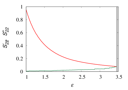
Figure 5: $S_{2,2}^{-}$ (lower curve) and $S_{2,2}^{+}$ (upper curve) vs $\varepsilon$ for the Plyukhin system discussed in the main text. The vertical line marks the value of $\varepsilon^{*}$.

To complete the description of this case, figure 6 depicts the velocity autocorrelation function $C_{vv}(t)$ vs $t$ obtained from stochastic simulations of the Plyukhin dynamics for a value of $\varepsilon$ close to $\varepsilon^{**}$, compared with the autocorrelation profile at the ergodicity-breaking threshold, i.e. at $\varepsilon^{*}$. Given a stochastic realization, i.e. an admissible positive semidefinite matrix derived from the moment equations at steady state, the stochastic intensity matrix $\bm{\beta}$ is obtained, by assuming its symmetric nature, from the equation $\bm{\beta}={\bf S}^{1/2}$, that admits always a symmetric solution if ${\bf S}$ is positive definite procopio .

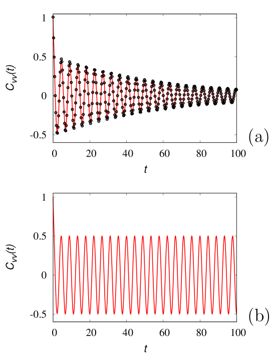
Figure 6: Velocity autocorrelation function $C_{vv}(t)$ for the Plyukhin model. Panel (a) refers to $\varepsilon=3.205$. Symbols ($\circ$) represent the results of stochastic simulations, the solid line corresponds to the solution deriving from the fluctuation-dissipation relations of the first kind. Panel (b) refers to $\varepsilon=\varepsilon^{*}$, i.e. to the critical condition for ergodicity breaking.

V Concluding remarks

The interpretation of the phenomenon of ergodicity breaking for GLE with well-behaved dissipative memory kernels within the broader dynamic theory of GLE permits not only to appreciate better its dynamic origin, but also to set conditions upon its physical manifestation.

By considering that in general the domain of stochastic realizability falls properly within the domain of dissipative stability, the phenomenon of ergodicity breaking for well-behaved dissipative kernels cannot be observed from the solution of the associated stochastic differential equations, and ultimately in physical systems. This statement has been proved for systems with kernel possessing two real exponents, and this result can be generalized in the case of a larger number of decaying real modes for which $h(t)$ is for any $t>0$ greater than zero. The Plyukhin model falls at the boundary of this analysis. But, apart from its mathematical and conceptual interest, its physical validity should be further addressed and discussed, in order to ascertain whether it may represents a realistic model for a physically realizable dynamics. Independently of this physical consistency check, its conceptual relevance remains unaltered.

From the analysis developed in this article the importance of the dynamic constraints in the analysis of GLE becomes evident: dissipative stability (and the cases of ergodicity breaking analyzed by Bao, Plyukhin et al., represent a beautiful and conceptually important example of it), and stochastic realizability. A further remark on the latter property is important.

While dissipative stability is a property pertaining to the mean-field deterministic contribution to the dynamics, and outside the region of dissipative stability the system does not admit an equilibrium behavior, stochastic realizability is a more stringent condition (in most of the cases, as seen via the model systems considered in this work) but, in the way it is defined, it is based on a physical assumption, namely the validity of the Langevin condition eq. (4). The Langevin condition motivates the use of white-noise processes in the representation of the thermal force, and is one-to-one with the expression for the velocity autocorrelation function stemming from the Kubo’s fluctuation-dissipation relation of the first kind. In other words, the definition of stochastic realizability adopted here is grounded on the validity of the Kubo theory. The Langevin condition is not a fundamental principle of physics as the constant value of the velocity of light in vacuo. It has represented an important condition to handle Brownian motion in fluids (gas and liquids) in a given range of pressures and temperatures close to the ambient ones. But in principle it can be violated, and its violation may lead to enlarge our understanding of fluctuational phenomena beyond the actual range. In the eventuality of such an extension, the definition of stochastic realizability should be generalized accordingly.

References

- (1) R. Kubo, Rep. Prog. Phys. 29 255 (1966).
- (2) R. Kubo, M. Toda and N. Hashitsune, Statistical Physics II Nonequilibrium Statistical Mechanics (Springer-Verlag, Berlin, 1991).
- (3) O. Darrigol, Eur. Phys. J. H 48 10 (2023).
- (4) P. Langevin, C. R. Acad. Sci. (Paris) 146 530 (1908); english translation in Am. J. Phys. 65 1079 (1997).
- (5) G. Procopio and M. Giona, Fluids 8 84 (2023).
- (6) C. W. Makosko, Rheology - Principles, Measurements, and Applications (Wiley-VCH, New York, 1994).
- (7) J. D. Ferry, Viscoelastic Properties of Polymers (J. Wiley & Sons, New York, 1970).
- (8) M. Grimm, S. Jeney and T. Franosch, Soft Matter 7, 2076 (2011).
- (9) I. Goychuk Adv. Chem. Phys. 150, 187 (2012).
- (10) I. Goychuk, Phys. Rev. E 80 046125 (2009).
- (11) P. Siegle, I. Goychuk and P. Hänggi, EPL 93 20002 (2011).
- (12) J.-D. Bao, P Hänggi and Y.-Z. Zhuo, Phys. Rev. E 72 061107 (2005).
- (13) J.-D. Bao, Eur. Phys. J. B 93 184 (2020).
- (14) A. V. Plyukhin, Phys. Rev. E 83 062102 (2011).
- (15) F. Ishikawa and S. Todo, Phys. Rev. E 98 062140 (2018).
- (16) A. V. Plyukhin, Phys. Rev. W 105 014121 (2022).
- (17) M. Giona, G. Procopio and C. Pezzotti, Dynamic fluctuation-dissipation theory for Generalized Langevin Equations: constructive constraints, stability and realizability, in preparation (2024).
- (18) L. D. Landau and E. M. Lifshitz, Fluid Mechanics; (Pergamon Press, Oxford, 1993).
- (19) N. G. van Kampen, Stochastic Processes in Physics and Chemistry (Elsevier, Amsterdam, 2007).
- (20) G. Procopio and M. Giona, Fluids 7 105 (2022).