Dynamic fluctuation-dissipation theory for Generalized Langevin Equations: constructive constraints, stability and realizability

Abstract

Using the initial-value formulation, a dynamic theory for systems evolving according to a Generalized Langevin Equation is developed, providing more restrictive conditions on the existence of equilibrium behavior and its fluctuation-dissipation implications. For systems fulfilling the property of local realizability, that for all the practical purposes corresponds to the postulate of the existence of a Markovian embedding, physical constraints, expressed in the form of dissipative stability and stochastic realizability are derived. If these two properties are met, Kubo theory is constructively recovered, while if one of these conditions is violated a thermodynamic equilibrium behavior does not exist (and this occurs also for “ well-behaved dissipative systems” according to the classical Kubo theory), with significant implications in the linear response theory.

Introduction - The fluctuation-dissipation (FD) theorems developed by Kubo for Generalized Langevin Equations (GLE) kubo1 ; kubo2 constitute a cornerstone in statistical physics admitting a huge variety of applications in all the branches of physics, microhydrodynamics and transport theory, electrochemistry and dieletric response, abstract linear response theory, etc. hydro1 ; gen1 ; gen2 , and cellular biology cell1 ; cell2 , involving thermal fluctuations.

In its original formulation kubo1 , the Kubo theory addresses the generalization of the equation of motion of a spherical Brownian particle of mass $m$ and velocity $v(t)$ in a fluid at thermal equilibrium (constant temperature $T$), in which the dissipative response of the fluid is not instantaneous but is described via a memory kernel $h(t)$

$$m\,\frac{dv(t)}{dt}=-\int_{-\infty}^{t}h(t-\tau)\,v(\tau)\,d\tau+R(t)$$ (1)

where $R(t)$ is the stochastic termal force, such that the resulting velocity process $v(t)$ is stationary. Another basic assumption for $R(t)$ is the Langevin condition, originally proposed by P. Langevin in 1908 langevin , stating that

$$\langle R(t)\,v(\tau)\rangle_{\rm eq}=0\qquad\tau\leq t$$ (2)

where $\langle\cdot\rangle_{\rm eq}$ is the expected value with respect to the probability measure of the thermal fluctuations at equilibrium. Eq. (2) implies that the stochastic force $R(t)$ at time $t$ is independent of the previous history of particle velocity. An alternative view to eq. (2) has been developed in felder (see also bala for a critical discussion).

The Kubo FD theory is developed in two steps: the determination of the velocity autocorrelation function $C_{vv}(t)=\langle v(t+\tau)\,\langle v(\tau)\rangle_{\rm eq}=\langle v(t)\,v(0)\rangle_{\rm eq}$ (due to stationarity), and this is referred to as the fluctuation-dissipation theorem of the first kind (FD1k, for short), and the determination of the autocorrelation function $C_{RR}(t)=\langle R(t)\,R(0)\rangle$ for the thermal force, referred to as the fluctuation-dissipation theorem of the second kind (FD2k, for short). The development of the Kubo theory starts from eq. (1) and involves essentially Fourier analysis, specifically the application of the Wiener-Khinchin theorem for stationary stochastic processes, imposing: (i) the Langevin condition eq. (2) and (ii) the value of the intensity of velocity fluctuations at thermal equilibrium,

$$\langle v^{2}\rangle_{\rm eq}=\frac{k_{B}\,T}{m}$$ (3)

where $k_{B}$ is the Boltzmann constant. We prefer to use the wording “properties” instead of ”theorems”, as FD1k and FD2k are two “properties” based upon specific physical assumptions (valid for some systems, but that can be equally well be violated by others), rather that propositions involving mathematical entities.

It is possible to frame the same problem in a slightly different way, replacing eq. (1) with

$$m\,\frac{dv(t)}{dt}=-\int_{0}^{t}h(t-\tau)\,v(\tau)\,d\tau+R(t)$$ (4)

equipped with the initial condition $v(0)=v_{0}$. The comparison of these two equations shows that the only difference between them refers to the lower integration value, that is $\tau=-\infty$ in eq. (1) that is turned to $\tau=0$ in eq. (4). Probably because of the apparent “tininess” of this difference, no great attention has been focused on it, and in the literature these two formulations are used interchangeably depending upon practical convenience lit1 ; lit2 ; lit3 ; lit4 . Henceforth we refer to eq. (1) as the abstract formulation of the GLE and to eq. (4) as its initial-value formulation.

In point of fact, the mathematical structure of these two formulations is different (although intrinsic analogies exist jap ; jap1 ), and more importantly this difference admits relevant implications as regards the methodological way of developing FD theory and the results following from it. The abstract formulation is essentially focused at determining the statistical properties of the stochastic processes $v(t)$ and $R(t)$ at equilibrium. In this way, it fits the purposes of an equilibrium theory for the linear response of physical systems to perturbations (Kramers-Krönig relations, analysis of susceptibilities, etc.) kubo2 ; degroot . As it represents intrinsically an equilibrium formulation, it is unable to handle neither the momentum relaxation dynamics and the convergence towards mechanical equilibrium nor any experiments in which a particle, possessing initially a velocity $v_{0}$, is injected into the fluid at some initial time, say $t=0$. Conversely, the initial-value formulation is a dynamic, non-equilibrium (as regards momentum transfer, not thermal effects) description of the process, i.e. of the hydromechanical interactions between the particle and the fluid. It corresponds to the description of experiments involving a particle (or a system of independent particles), injected into the fluid and relaxing its momentum dynamics towards equilibrium conditions, providing a stochastic evolution equation for the particle velocity, the results of which can be directly checked against experiments such as those involving Brownian motion exp0 ; exp1 ; exp2 ; exp3 . For the sake of physical correctness, eq. (4) describes the fluid-particle interactions in a viscous fluid neglecting fluid-inertial effects franosch ; procopiovisco , in which the memory kernel $h(t)$ accounts for the viscoelastic dissipative properties of the fluid rheol1 ; rheol2 .

The Kubo FD theory has been developed starting from eq. (1) and there is no direct proof of it starting from eq. (4). The present Letter is aimed at developing the necessary technical tools for a FD theory starting from eq. (4), and derive the physical implications. This change of perspective permits to derive new and apparently unexpected properties of FD theory, associated with its physical realizability, existence of equilibrium properties, and ultimately applicability of the Stokes-Einstein relation for simple and “well-behaved” dissipative memory kernels. The concept of local realizability of the memory kernel, dissipative stability of the GLE, and stochastic realizability for the thermal fluctuations are introduced as necessary constraints corresponding to thermodynamic consistency conditions. Depending on their fulfillment several different regimes are observed and explained. The results obtained are not only consistent with the mathematical theory of linear integrodifferential equations math1 ; math2 , but also show unexpected features once compared and contrasted against the classical FD theory: in apparently “simple well-behaved dissipative” systems (see further for a definition), for which the classical Kubo theory predicts a regular diffusive behavior satisfying Stokes-Einstein relations, the present theory correctly predicts and explains the violation of the Stokes-Einstein relation as a consequence of the lack of any thermodynamic equilibrium behavior. Moreover, the present theory provides a simple interpretation of the phenomena associated with ergodicity breaking of simple dissipative GLE in the presence of memory kernels exponentially decaying in time bao1 ; bao2 ; bao3 ; plyukhin1 ; plyukhin2 . For a thorough analysis of this case see ergbreak . The present approach constitutes a necessary complement and a significant refinement of the linear response theory as regards thermodynamic consistency of the memory kernels and of their interaction with equilibrium fluctuations.

FD1k and FD2k - To begin with, consider FD1k. This follows directly from eq. (4) as a consequence of the Langevin condition eq. (2), multiplying it by $v(0)$ and taking the expected value with respect to the equilibrium probability measure:

$$m\,\frac{d\langle v(t)\,v(0)\rangle_{\rm eq}}{dt}=m\,\frac{dC_{vv}(t)}{dt}=-\int_{0}^{t}h(t-\tau)\,C_{vv}(\tau)\,d\tau$$ (5)

equipped with the initial condition $C_{vv}(0)=\langle v^{2}\rangle_{\rm eq}$. In the Laplace domain, setting $\widehat{h}(s)=L[h(t)]=\int_{0}^{\infty}e^{-st}\,h(t)\,dt$, and similarly for the other functions, the solution of eq. (5) is

$$\widehat{C}_{vv}(s)=\frac{\langle v^{2}\rangle}{s+\widehat{h}(s)/m}=\langle v^{2}\rangle\,\widehat{G}(s)$$ (6)

where $\widehat{G}(s)$ is the Laplace transform of the Green function (referred to as the resolvent in math1 associated with the memory dynamics defined by $h(t)$).

Elaborating further the structure of the stochastic perturbation (see the Appendices), it is possible to derive the following condition

$$\int_{0}^{\infty}G(\tau)\,\left[k_{B}\,T\,h(\tau)-C_{RR}(\tau)\right]\,d\tau=0$$ (7)

where $G(t)=L^{-1}[\widehat{G}(s)]$ is the resolvent function defined by eq. (6). Eq. (7) is the most general FD2k result associated with the analysis of the kinetic energy for the initial value GLE. It will be referred to as the weak formulation of FD2k. Of course, if

$$C_{RR}(t)=k_{B}\,T\,h(t)$$ (8)

corresponding to the Kubo FD2k for abstract GLE, eq. (7) is identically satisfied, but we cannot claim eq. (8) directly from eq. (7).

Local realizability - In order to improve the analysis, a further condition on the GLE should be posed. Indeed, a solution to this problem is provided by the assumption of local realizability, introduced below. Consider again the memory term $-h(t)*v(t)$ in eq. (4) where “$*$” stands for convolution, corresponding to the force exerted by the fluid on the particle at time $t$, and a continuous kernel $h(t)$ (i.e. not impulsive as in the case of the Stokes-Einstein kernel, $h(t)=\eta\,\delta(t)$). This action is local in time, in the meaning that it should be properly viewed as the lumped and compact mathematical representation of local effects, occurring instantaneously in time, i.e. at time $t$. This means that a vector-valued $n$-dimensional function ${\bf z}(t)$ of time and a scalar function $\psi:{\mathbb{R}}^{n}\rightarrow{\mathbb{R}}$ should exist, such that $-h(t)*v(t)=\psi({\bf z}(t))$, where ${\bf z}(t)$ evolves according to a differential equation $d{\bf z}(t)/dt={\bf f}({\bf z}(t),v(t),t)$.

But eq. (4) is linear and it gives rise to a stationary stochastic process $v(t)$. This implies that the vector field ${\bf f}({\bf z}(t),v(t),t)$ should be linear in both ${\bf z}(t)$ and $v(t)$ and autonomous (time-independent), and $\phi({\bf z}(t))$ a linear (and homogeneous) functional of ${\bf z}(t)$. Consequently, the memory term entering eq. (4) should be the expressed as the linear projection of the local functions ${\bf z}(t)=(z_{1}(t),\dots,z_{n}(t))$, be their system finite or countable, where ${\bf z}(t)$ satisfies an ordinary linear differential equation with constant coefficients driven by stochastic fluctuations, that can be expressed as a linear combination of white noise processes (by eq. (2)).

We thus arrive at the definition of local realizability. The GLE is said to be locally realizable if there exist a constant $n\times n$ matrix $\bm{\Lambda}$ and a constant $n$-vector ${\bf a}$ such that eq. (4) for $R(t)=0$ can be expressed as the projection with respect to ${\bf a}$ of an $n$-dimensional process of internal degrees of freedom ${\bf z}(t)$,

$$m\,\frac{dv(t)}{dt}=-\sum_{h=1}^{n}a_{i}\,z_{i}(t)=-\left({\bf a},{\bf z}(t)\right)$$ (9)

evolving according to the local dynamics

$$\frac{d{\bf z}(t)}{dt}=-\bm{\Lambda}\,{\bf z}(t)+{\bf 1}\,v(t)$$ (10)

where ${\bf 1}=(1,\dots,1)$. From the mathematical point of view, local realizability is one-to-one with the property that $h(t)$ possesses a finite or countable number of pole singularities. It follows from this definition that

$$h(t)=\left({\bf a},e^{-\bm{\Lambda}\,t}\,{\bf 1}\right)$$ (11)

The GLE is stocastically realizable if there exists a constant $n\times n$ matrix $\bm{\beta}$ such that eq. (4) can be expressed by eq. (9) with

$$\frac{d{\bf z}(t)}{dt}=-\bm{\Lambda}\,{\bf z}(t)+{\bf 1}\,v(t)+\sqrt{2}\,\bm{\beta}\,\bm{\xi}(t)$$ (12)

where $\bm{\xi}(t)=(\xi_{1}(t),\dots,\xi_{n}(t))$ is a vector-valued white noise process vankampen , $\langle\xi_{i}(t)\,\xi_{j}(\tau)\rangle=\delta_{ij}\,\delta(t-\tau)$, and eqs. (9), (12) admit an equilibrium invariant measure for which eqs. (3) and (5) hold (i.e. FD1k is verified). In practice, one may choose $\xi_{i}(t)=dw_{i}(t)/dt$, where $w_{i}(t)$ are independent Wiener processes.

It is easy to observe that local realizability involves exclusively the dissipative contribution, while stochastic realizability corresponds to the existence of a Markov embedding of eq. (4), and specifically the existence of a stochastic process $R(t)$, with the property of fulfilling the Langevin condition eq. (2) and in turn eqs. (3), (5).

Without loss of generality, assume that the internal degrees of freedom $z_{i}(t)$ are expressed in the eigenbasis of $\bm{\Lambda}$ so that $\bm{\Lambda}=\mbox{diag}(\lambda_{1},\dots,\lambda_{n})$. Assume $\lambda_{i}\in{\mathbb{R}}$, with $\lambda_{i}>0$, that corresponds to the dissipative friction factor in viscoelastic fluids rheol1 ; rheol2 . At the moment consider the case where $a_{i}>0$, $i=1,\dots,n$, as dictated by the rheological analysis rheol1 ; rheol2 . In this case, eq. (10) takes the simpler form $h(t)=\sum_{i=1}^{n}a_{i}\,e^{-\lambda_{i}\,t}$.

To begin with, assume that the stochastic fluctuations acting on the internal models are characterized by the commutative property $[\bm{\Lambda},\bm{\beta}]=\bm{\Lambda}\bm{\beta}-\bm{\beta}\bm{\Lambda}=0$, and consequently the matrix $\bm{\beta}$ is also diagonal once expressed in the eigenbasis of $\bm{\Lambda}$, $\bm{\beta}=\mbox{diag}(c_{1},\dots,c_{n})$.

Under these hypotheses, eqs (8), (12) admit an equilibrium invariant measure, and FD1k, i.e. eq. (5), is fulfilled provided that the conditions

$$\langle z_{i}\,v\rangle_{\rm eq}=0\,,\qquad i=1,\dots,n$$ (13)

are met (see the Appendices), indicating that the internal variables $z_{i}(t)$ should be uncorrelated from the velocity $v(t)$ at equilibrium. Enforcing eq. (3), the expression for the coefficients $c_{i}$ follows

$$c_{i}^{2}=m\,\langle v^{2}\rangle\,\frac{\lambda_{i}}{a_{i}}\,,\qquad i=1,\dots,n$$ (14)

consistently with the analysis developed by Goychuk goychuk . Since the process $R(t)$ attains at equilibrium the expression $R(t)=-\sqrt{2}\,\sum_{i=1}^{n}a_{i}\,c_{i}\,e^{-\lambda_{i}\,t}*\xi_{i}(t)$, from eq. (12) it readily follows that (see the Appendices)

$$C_{RR}(t)=k_{B}\,T\,\sum_{i=1}^{n}a_{i}e^{-\lambda_{i}\,t}=k_{B}\,T\,h(t)$$ (15)

i.e. that FD2k in its strong form is verified.

Consistency conditions: Thermodynamic equilibria and FD failures - Before considering the case of negative $a_{i}^{\prime}s$, let us address a preliminary observation. FD theory applies if a thermodynamic equilibrium state exists, which is a property that cannot be given for granted for GLE, even involving “well-behaved” dissipative kernels. The latter property can be defined by the conditions: (i) $h(t)\geq 0$; (ii) $h(t)\in L_{1}([0,\infty))$, and thus $0<\eta_{\infty}=\int_{0}^{\infty}h(t)dt<\infty$; (iii) $h(t)$ is exponentially decaying with time $t$ (for large $t$). In the classical FD theory property (i)+(ii) ensures that the Laplace-Fourier transform of $h(t)$ exists, and that the effective diffusivity $D$ fulfils the generalized Stokes-Einstein relation $D=\widehat{C}_{vv}(0)=k_{B}\,T/\eta_{\infty}$. But this is not true in general. Let us consider a simple example and derive out of it some general conclusions. Consider a non-dimensional formulation of the GLE which implies that we can set in eq. (4) $m=1$, and $\langle v^{2}\rangle_{\rm eq}=1$, and a simple two-mode kernel

$$h(t)=a_{1}\,e^{-\lambda_{1}t}+a_{2}\,e^{-\lambda_{2}t}$$ (16)

with $a_{1}=1$, $a_{2}=-\alpha$, $\lambda_{1}=1/10$, $\lambda_{2}=1$, where $\alpha\leq 1$ is taken as a parameter. The graphs of $h(t)$ for several values of $\alpha$ are depicted in figure 4.

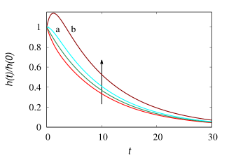
Figure 1: $h(t)/h(0)$ vs $t$ for the model considered in the main text. The arrow indicates increasing values of $\alpha=-0.1,\,0,\,0.1,\,0.3$. Line (a) refers to $\alpha=0.1$, line (b) to $\alpha=0.3$.

For these kernels, the conditions (i)-(iii) stated above are met and $\eta_{\infty}=a_{1}/\lambda_{1}+a_{2}/\lambda_{2}=10-\alpha$. Setting ${\bf y}=(v,z_{1},z_{2})$ the overall dynamics eqs. (9)-(12) can be compactly expressed as $d{\bf y}/dt={\bf A}\,{\bf y}+\sqrt{2}\,\bm{\beta}\,\bm{\xi}$, where the coefficient matrix ${\bf A}$ is given by

$${\bf A}=\left(\begin{array}[]{ccc}0&-a_{1}&\alpha\\ 1&-\lambda_{1}&0\\ 1&0&-\lambda_{2}\end{array}\right)$$ (17)

The eigenvalue spectrum of ${\bf A}$ controls the dynamic response of the system. For $\alpha\in(-\infty,\alpha_{\rm ds})={\mathcal{D}}_{\rm ds}$, with $\alpha_{\rm ds}=0.21$ all the eigenvalues possess negative real part: for $\alpha\in(0,\alpha_{\rm ds})$ there exists a real eigenvalue and a couple of complex conjugate eigenvalues. Above $\alpha_{\rm ds}$, the real part of the complex-conjugate pair becomes positive, while the real eigenvalue remains negative. Therefore, for $\alpha>\alpha_{\rm ds}$ the stochastic dynamics is unstable and the system does not attain an equilibrium behavior, as the fluctuations cannot be restricted to the stable eigenspace of ${\bf A}$. We refer to ${\mathcal{D}}_{\rm ds}=(-\infty,\alpha_{\rm ds})$ as to the region of dissipative stability of the GLE. Outside ${\mathcal{D}}_{\rm ds}$ no thermodynamic equilibrium exists, because the “dissipative” dynamics of the GLE is unstable.

This result follows also from the general theory of linear integro-differential equations math1 ; math2 : the condition for asymptotic stability of eq. (4) is that $(m\,s+\widehat{h}(s))\neq 0$ for $\mbox{Re}[s]\geq 0$, corresponding to the absence of eigenvalues of ${\bf A}$ with positive real part. In this regard, the occurrence of instabilities in GLE with “well-behaved” kernels goes beyond the assumption of local realizability of $h(t)$. For GLE with “well-behaved” kernels that are not dissipatively stable, the Fourier-Laplace transform of $h(t)$ is defined outside the half-plane of convergence of $\widehat{h}(s)$ (that is $\mbox{Re}[s]>\mu_{\rm max}>0$, with $\mu_{\rm max}>0$ the largest positive real part of the eigenvalues of ${\bf A}$) and, as a consequence, it neither describes the response to external perturbations (for instance periodic ones) nor it permits to derive the expression for the diffusivity (that in these situations simply does not exist). As a further remark, the problem of ergodicity breaking considered in bao1 ; bao2 ; bao3 ; plyukhin1 ; plyukhin2 corresponds to conditions on the kernel lying at the boundary of the region of dissipative stability ergbreak .

We can use further eq. (16) as a model for unveiling the constructive structure of the FD theory. From what said above, the region $\alpha\in{\mathcal{D}}_{\rm c}=(-\infty,0]\subset{\mathcal{D}}_{\rm ds}$, and consequently an equilibrium state exists. Moreover, we have obtained constructively that the matrices $\bm{\Lambda}$ and $\bm{\beta}$ commute, and that the FD theory applies. Let $\alpha_{\rm c}=0$ be the upper value of $\alpha$ in this region.

For $\alpha\in(\alpha_{\rm c},\alpha_{\rm ds})$ the eigenrepresentation of $\Lambda$ does not diagonalize $\bm{\beta}$, and therefore $\bm{\beta}$ should be a full matrix. The mathematical details are developed in the Appendices, and rely on the properties of $\bm{\beta}$. It is shown that for $\alpha=(\alpha_{\rm c},\alpha_{\rm nc})$ with $\alpha_{\rm nc}=0.1$, a non-diagonal matrix $\bm{\beta}$ can always be defined, such that FD1k and FD2k are verified. Conversely, for $\alpha\in(\alpha_{\rm nc},\alpha_{\rm ds})$ there is no stochastic model consistent with the FD1k eq. (5) although, for any choice of $\bm{\beta}$, the stochastic dynamics eqs. (9),(12) admits a stationary non-equilibrium invariant measure. For $\alpha={\mathcal{D}}_{sr}=(-\infty,\alpha_{nc})$ the GLE is stochastically realizable and this means that: (i) the GLE is not unstable, and (ii) a model for the thermal force can be realized such that the corresponding stationary measures/fluctuations correspond to those in thermal equilibrium conditions. It follows from (i) that ${\mathcal{D}}_{sr}\subseteq{\mathcal{D}}_{\rm ds}$, (ii) $\alpha_{\rm c}\leq\alpha_{\rm nc}\leq\alpha_{\rm ds}$, and consequently the FD theory applies for kernels belonging to ${\mathcal{D}}_{sr}$. To make a numerical example, figure 5 (upper panel) depicts the velocity autocorrelation functions for $\alpha=0.08\in{\mathcal{D}}_{\rm sr}$ (inner dots), and the “ideal” Kubo autocorrelation function $C_{vv}^{(K)}(t)$ solution of eq. (5) for $\alpha=0.18$ (curve a) outside ${\mathcal{D}}_{\rm sr}$ but still inside ${\mathcal{D}}_{ds}$ that, from what said above, cannot be realized by any stochastic model consistent with eqs. (3), (5). The lower panel corresponds to $C_{vv}^{(K)}(t)$ for $\alpha=0.3$, outside ${\mathcal{D}}_{\rm ds}$, for which $|C_{vv}^{(K)}(t)|\sim e^{\mu_{\rm max}\,t}$ where $\mu_{\rm max}\simeq 0.0214$.

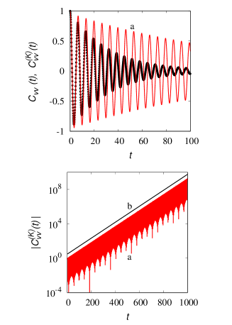
Figure 2: Upper panel: $C_{vv}(t)$ (symbols) for $\alpha=0.08$ and $C_{vv}^{(K)}(t)$ for $\alpha=0.18$ vs $t$. Lower panel: $C_{vv}^{(K)}(t)$ (line a) for $\alpha=0.3$ vs $t$. Line (b) corresponds to the exponential scaling $e^{\mu_{\rm max}\,t}$.

The properties of “well-behaved” kernels in the region outside ${\mathcal{D}}_{\rm ds}$ admits relevant implications in the linear response theory. Specifically, if $h(t)$ possesses real poles with negative real part this does not imply that its response to a sinusoidal perturbation ${\bf F}(\omega)=F_{0}e^{\pm\mathrm{i}\omega\,t}$ would be bounded and described by the mobility function $\mu(\omega)=1/(i\omega+h[\omega]$) kubo2 , where $h[\omega]=\widehat{h}(\mathrm{i}\,\omega)$, $\mathrm{i}=\sqrt{-1}$. Generically we have an exponentially diverging dynamics with time $t$, where $|v(t)|\leq\mu_{c}^{(e)}(\omega)\,F_{0}\,e^{\mu_{\rm max}\,t}$, if $F(\omega)=F_{0}\,\cos(\omega\,t)$, and $|v(t)|\leq\mu_{s}^{(e)}(\omega)\,F_{0}\,e^{\mu_{\rm max}\,t}$, if $F(\omega)=F_{0}\,\sin(\omega\,t)$, with obviously $\mu_{s}^{(e)}(\omega)\neq\mu_{c}^{(e)}(\omega)$. The graph of these functions is depicted in figure 6 for $\alpha=0.3$. In these cases, i.e. for dissipatively unstable systems, the classical linear response theory should be revisited. It follows straightforwardly that, outside ${\mathcal{D}}_{\rm ds}$ no Stokes-Einstein relations can be defined, albeit $\eta_{\infty}=\int_{0}^{\infty}h(t)\,dt>0$ may exist.

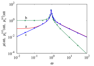
Figure 3: $\mu(\omega)$ line (a), $\mu_{c}^{(e)}(\omega)$ line (b), and $\mu_{s}^{(e)}(\omega)$ line (c) predicted analytically (see the Appendices). Symbols, are the results of numerical simulations.

Concluding remarks - The theory above developed provides clear thermodynamic conditions to be set for the memory response function $h(t)$ of physical equilibrium systems. In order to be thermodynamically consistent, $h(t)$ should be: dissipatively stable, as otherwise it is meaningless to assume the occurrence of stationary properties (and a-fortiori the existence of an equilibrium state), and (ii) stochastically realizable, as otherwise the steady states do not correspond to thermodynamic equilibrium conditions driven by stochastic fluctuations. The first property involves exclusive the dissipative dynamics, i.e. the kernel $h(t)$. The condition of stochastic realizability provides a constructive and definite limit to the FD theory. The application of FD theory for systems outside the region ${\mathcal{D}}_{sr}$ is not only mathematically incorrect, but also may lead to completely erroneous physical predictions. Retrospectively, the “wormhole” of the classical FD theory based on eq. (1) appears clear: since it assumes the occurrence of thermodynamic equilibrium conditions without assessing them, it fails whenever the equilibrium conditions cannot occur either by dissipative instability or by the lack of stochastic realizability. This shortcoming cannot occur within the initial-value formulation of FD theory, as it is grounded on a constructive approach to FD2k. This is the principal methodological difference in the two approaches, as from the mathematical point of view the conditions assessing the asymptotic stability of eq. (4) are fully equivalent to those for eq. (1) jap . The analysis of the dissipative stability of “well-behaved kernels”, such as those defined by eq. (16), indicates further that the physical meaning of dissipation is much more subtle either than the existence of a positive and finite value of $\eta_{\infty}>0$ and $\mbox{Re}[\lambda_{i}]>0$, or than the condition $\mbox{trace}({\bf A})<0$, as it necessarily involves a description of the internal dynamics in order to assess its thermodynamic plausibility. Moreover, it is possible to show the breakdown of the constraints of dissipative stability and stochastic realizability ever for monotonically non-increasing kernels, i.e. such that $dh(t)/dt\leq 0$ for all $t\geq 0$. This hinges towards a constructive approach to FD theory grounded on the explicit representation of $R(t)$ in terms of stochastics processes, as developed above. A thorough elaboration of the dynamic theory of GLE will be developed in a longer communication, with particular emphasys to hydromechancal interactions and Brownian motion and to the Debye relaxation mechanism debye1 ; debye2 .

Appendix I - Kinetic energy balance - Kinetic energy balances represent a convenient way to approach FD2k starting from the initial-value representation. To begin with, consider the classical memoryless Langevin model for a Brownian spherical particle, where the thermal force is proportional to the distributional derivative of a Wiener process $R(t)=\alpha\,dw(t)/dt$,

$$m\,dv(t)=-\eta\,v(t)\,dt+\alpha\,dw(t)$$ (18)

and $\eta$ is the friction factor. Consider the evolution equation for the kinetic energy. Due to the singular nature of eq. (18), the Ito lemma can be applied,

$$\frac{m}{2}dv^{2}(t) = m\,v(t)\,dv(t)+\frac{m}{2}\left(dv(t)\right)^{2}$$ (19)

$$= -\eta\,v^{2}(t)\,dt+\alpha\,v(t)\,dw(t)+\frac{\alpha^{2}}{2\,m}\,dt+o(dt)$$

Taking the expected value of both sides of eq. (19) with respect to the probability measure of the fluctuations at equilibrium, enforcing the Langevin condition, i.e. $\langle v(t)\,dw(t)\rangle=0$, and considering that at equilibrium $d\,\langle v^{2}\rangle_{\rm eq}=0$, we obtain to the $dt$-order, $-\eta\,\langle v^{2}\rangle+\alpha^{2}/2\,m=0$, leading to $\alpha=\sqrt{2\,k_{B}\,T\,\eta}$.

The same approach can be applied to the GLE. Due to the convolutional nature of the dissipation term, it is natural to consider a convolutional expression for $R(t)$, i.e.,

$$m\,\frac{dv(t)}{dt}=-\int_{0}^{t}h(t-\tau)\,v(\tau)\,d\tau+\int_{0}^{t}\gamma(t-\tau)\,\xi(\tau)\,d\tau$$ (20)

where $\xi(t)$ is the distributional derivative of a Wiener process, and $\gamma(t)$ a smooth memory kernel. In this case, the stochastic force is given by $R(t)=\int_{0}^{t}\gamma(t-\tau)\,\xi(\tau)\,d\tau$, and its autocorrelation function can be expressed as

$$C_{RR}(t)=\langle R(t)\,R(0)\rangle=\int_{0}^{\infty}\gamma(t+\tau)\,\gamma(\tau)\,d\tau$$ (21)

Similarly to the impulsive case, one can to derive FD2k by considering the evolution of the kinetic energy. From eq. (20) we obtain

$$\frac{m}{2}\,\frac{d\langle v^{2}(t)\rangle}{dt} = -\int_{0}^{t}h(t-\tau)\,\langle v(\tau)\,v(t)\rangle\,d\tau+\int_{0}^{t}\gamma(t-\tau)\,\langle\xi(\tau)\,v(t)\rangle\,d\tau$$

$$= -\int_{0}^{t}h(t-\tau)\,C_{vv}(t-\tau)\,d\tau+\int_{0}^{t}\gamma(t-\tau)\,C_{v\xi}(t-\tau)\,d\tau$$

$$= -\int_{0}^{t}h(\tau)\,C_{vv}(\tau)\,d\tau+\int_{0}^{t}\gamma(\tau)\,C_{v\xi}(\tau)\,d\tau$$

that has been derived by enforcing the property that $v(t)$ is a stationary stochastic process. At equilibrium, i.e. for $t\rightarrow\infty$, the l.h.s. of eq. (Dynamic fluctuation-dissipation theory for Generalized Langevin Equations: constructive constraints, stability and realizability) is vanishing, and this implies

$$\int_{0}^{\infty}h(\tau)\,C_{vv}(\tau)\,d\tau=\int_{0}^{\infty}\gamma(\tau)\,C_{v\xi}(\tau)\,d\tau$$ (23)

where $C_{vv}(t)=\langle v(t)\,v(0)\rangle_{\rm eq}$ and $C_{v\xi}(t)=\langle v(t)\,\xi(0)\rangle_{\rm eq}$ are the correlation functions at equilibrium conditions. The evolution equation for $C_{v\xi}(t)$ follows from eq. (20), multiplying it by $\xi(0)$ and taking the expect value

$$m\,\frac{dC_{v\xi}(t)}{dt}=-\int_{0}^{t}h(t-\tau)\,C_{v\xi}(\tau)\,d\tau+\gamma(t)$$ (24)

It is equipped with the initial condition $C_{v\xi}(0)=0$. Thus,

$$C_{vv}(t) = \langle v^{2}\rangle\,G(t)$$

$$C_{v\xi}(t) = \int_{0}^{t}G(t-\tau)\,\gamma(\tau)\,d\tau=\frac{1}{m}\,G(t)*\gamma(t)$$ (25)

where $G(t)$ is the Green function expressed by the inverse Laplace transform

$$G(t)=L^{-1}\left[\frac{1}{s+\widehat{h}(s)/m}\right]$$ (26)

Substituting eq. (25) into eq. (23) we have

$$m\,\langle v^{2}\rangle\int_{0}^{\infty}h(\tau)\,G(\tau)\,d\tau=\underbrace{\int_{0}^{\infty}\gamma(\tau)\,\left[\gamma*G(\tau)\right]\,d\tau}_{I}$$ (27)

The integral $I$ at the r.h.s of eq. (27) can be expressed as

$$I = \int_{0}^{\infty}\int_{0}^{\tau}\gamma(\tau-\theta)\,G(\theta)\,d\theta=\int_{0}^{\infty}G(\theta)\,d\theta\int_{\theta}^{\infty}\gamma(\tau)\,\gamma(\tau-\theta)\,d\tau$$ (28)

$$= \int_{0}^{\infty}G(\theta)\,\int_{0}^{\infty}\gamma(\tau+\theta)\,\gamma(\tau)\,d\tau=\int_{0}^{\infty}G(\theta)\,C_{RR}(\theta)\,d\theta$$

and therefore eq. (27) takes the final form

$$\int_{0}^{\infty}G(\tau)\,\left[k_{B}\,T\,h(\tau)-C_{RR}(\tau)\right]\,d\tau=0$$ (29)

corresponding to the weak formulation of the FD2k reported in the main text.

Appendix II - Stochastic realizations: the commutative case - This case corresponds to the mutual diagonalization of the dissipative and fluctuational contributions, (i.e. of the matrices $\bm{\Lambda}$ and $\bm{\beta}$). Here we outline the basic methodology used, while for the explicit calculations we refer to the next section, dealing with the more general condition $[\bm{\Lambda},\bm{\beta}]\neq 0$. Consider the expression for the kernel $h(t)$

$$h(t)=\sum_{i=1}^{n}a_{i}\,e^{-\lambda_{i}\,t}$$ (30)

with $\lambda_{i}>0$. To this kernel, assuming $[\bm{\Lambda},\bm{\beta}]=0$, corresponds the local representation of the GLE

$$\frac{dv(t)}{dt} = -\sum_{i=1}^{n}a_{i}\,z_{i}(t)$$

$$\frac{dz_{i}(t)}{dt} = -\lambda_{i}\,z_{i}(t)+v(t)+\sqrt{2}\,c_{i}\,\xi_{i}(t)\,,\quad i=1,\dots,n$$ (31)

where $\xi_{i}(t)$ can be taken as distributional derivatives of independent Wiener processes $w_{i}(t)$, $\xi_{i}(t)=dw_{i}(t)/dt$, $i=1,\dots,n$. In this way, the associated Fokker-Planck equation for the probability density $p(v,{\bf z},t)$, ${\bf z}=(z_{1},\dots,z_{n})$ is parabolic. The moments

$$\langle v^{2}(t)\rangle = \int v^{2}\,p(v,{\bf z},t)\,dvd{\bf z}$$

$$\langle z_{i}(t)\,v(t)\rangle = \int z_{i}\,v\,p(v,{\bf z},t)\,dvd{\bf z}=y_{i}(t)\,,\quad i=1,\dots,n$$ (32)

$$\langle z_{i}(t)\,z_{j}(t)\rangle = \int z_{i}\,z_{j}\,p(v,{\bf z},t)\,dvd{\bf z}=m_{i,j}(t)\,,\quad i,j=1,\dots,n$$

can be defined, where $d{\bf z}=dz_{1}\cdots dz_{n}$, and their evolution equations derived, equipped with arbitrary initial conditions associated with the initial preparation of the process, defined e.g. by any initial density $p_{0}(v,{\bf z})$, $p(v,{\bf z},t=0)=p_{0}(v,{\bf z})$. At equilibrium, if an equilibrum exists, the steady-state moment values are given by the equilibrium quantities $\langle v^{2}\rangle_{\rm eq}$, $\langle z_{i}\,v\rangle_{\rm eq}$, $\langle z_{i}\,z_{j}\rangle_{\rm eq}$, respectively.

Similarly, by enforcing the Langevin condition, it follows for the correlation functions $C_{vv}(t)$ and $C_{z_{i}v}(t)$ at equilibrium,

$$C_{vv}(t) = \langle v(t)\,v(0)\rangle_{\rm eq}=\lim_{\tau\rightarrow\infty}\langle(v(t+\tau)\,v(\tau)\rangle$$

$$C_{z_{i}v}(t) = \langle z_{i}(t)\,v(0)\rangle_{\rm eq}=\lim_{\tau\rightarrow\infty}\langle(z_{i}(t+\tau)\,v(\tau)\rangle\,,\qquad i=1,\dots,n$$ (33)

the system of evolution equations

$$\frac{dC_{vv}(t)}{dt} = -\sum_{i=1}^{n}a_{i}\,C_{z_{i}v}(t)$$

$$\frac{dC_{z_{i}v}(t)}{dt} = -\lambda_{i}\,C_{z_{i}v}(t)+C_{vv}(t)$$ (34)

equipped with the initial conditions,

$$C_{vv}(0)=\langle v^{2}\rangle_{\rm eq}\,,\qquad C_{z_{i}v}(0)=\langle z_{i}\,v\rangle_{\rm eq}\,,\quad i=1,\dots,n$$ (35)

From the second system of equations (34) we have

$$C_{z_{i}v}(t)=\langle z_{i}\,v\rangle_{\rm eq}\,e^{-\lambda_{i}\,t}+e^{-\lambda_{i}\,t}*v(t)\,,\qquad i=1,\dots,n$$ (36)

where we use the symbol “*” to indicate the convolution integral between any two functions $f(t)*g(t)=\int_{0}^{t}f(t-\tau)\,g(\tau)\,d\tau$. Substituting eqs. (36) into the first eq. (34) we obtain

$$\frac{dC_{vv}(t)}{dt}=-h(t)*C_{vv}(t)-\sum_{i=1}^{n}e^{-\lambda_{i}\,t}\langle z_{i}\,v\rangle_{\rm eq}$$ (37)

In order to recover the fluctuation-dissipation relation of the first kind (FD1k), that is a consequence of the Langevin condition, we should have identically

$$\langle z_{i}\,v\rangle_{\rm eq}=0\,,\qquad i=1,\dots,n$$ (38)

In the initial-value representation of the FD theory, the system of equations (38) represents the fundamental constraint imposed on the internal degrees of freedom, out of which the equilibrium FD theory can be developed. Specifically, from eq. (38), the expression for the intensity coefficients $c_{i}$ directly follows after elementary algebraic manipulations of the steady-state moment equations.

Appendix III - Stochastic realizations: the noncommutative case - In the main text we have considered the following kernel

$$h(t)=a_{1}\,e^{-\lambda_{1}\,t}+a_{2}\,e^{-\lambda_{2}\,t}$$ (39)

in nondimensional form (i.e. $m=1$ for the mass, and $\langle v^{2}\rangle_{\rm eq}=1$ for the velocity), with $a_{1}=1$, $a_{2}=-\alpha$, $\lambda_{1}=1/10$, $\lambda_{2}=1$. For positive values of $\alpha$, $\bm{\Lambda}$ and $\bm{\beta}$ cannot commute to produce an equilibrium behavior. Therefore, $\bm{\beta}$ should be a full matrix, and the local representation follows

$$\frac{dv(t)}{dt} = -a_{1}\,z_{1}(t)-a_{2}\,z_{2}(t)$$

$$\frac{dz_{1}(t)}{dt} = -\lambda_{1}\,z_{1}(t)+v(t)+\sqrt{2}\,\left(\beta_{1,1}\,\xi_{1}(t)+\beta_{1,2}\,\xi_{2}(t)\right)$$ (40)

$$\frac{dz_{2}(t)}{dt} = -\lambda_{2}\,z_{2}(t)+v(t)+\sqrt{2}\,\left(\beta_{2,1}\,\xi_{1}(t)+\beta_{2,2}\,\xi_{2}(t)\right)$$

Observe that the stochastic forcing cannot act directly on the velocity variable, as otherwise no equilibrium conditions could be achieved.

The Fokker-Planck equation for the density $p(v,z_{1},z_{2},t)$ associated with eq. (40) is

$$\frac{\partial p}{\partial t}=(a_{1}\,z_{1}+a_{2}\,z_{2})\frac{\partial p}{\partial v}+\sum_{i=1}^{2}\lambda_{i}\frac{\partial(z_{i}\,p)}{\partial z_{i}}-v\,\sum_{i=1}^{2}\frac{\partial p}{\partial z_{i}}+\sum_{i=1}^{2}\sum_{j=1}^{2}S_{i,j}\,\frac{\partial^{2}p}{\partial z_{i}\partial z_{j}}$$ (41)

where $\bm{\beta}=(\beta_{i,j})_{i,j=1,2}$, and the matrix ${\bf S}=(S_{i,j})_{i,j=1,2}$ is defined by

$${\bf S}=\bm{\beta}\,\bm{\beta}^{T}$$ (42)

where the superscript “$T$” indicate transpose. The matrix ${\bf S}$ should be positive definite. Componentwise,

$$S_{1,1}=\sum_{i=1}^{2}(\beta_{1,i})^{2}\,,\qquad S_{2,2}=\sum_{i=1}^{2}(\beta_{2,i})^{2}\,,\quad S_{1,2}=S_{2,1}=\sum_{i=1}^{2}\beta_{1,i}\,\beta_{2,i}$$ (43)

In this case, the moment equations read

$$\frac{d\langle v^{2}\rangle}{dt} = -a_{1}\,y_{1}-a_{2}y_{2}$$ (44)

$$\frac{dy_{i}}{dt} = -\sum_{j=1}^{2}a_{j}m_{i,j}-\lambda_{i}\,y_{i}+\langle v^{2}\rangle\,,\quad i=1,2$$ (45)

$$\frac{dm_{i,j}}{dt} = -(\lambda_{i}+\lambda_{j})\,m_{i,j}+y_{i}+y_{j}+S_{i,j}+S_{j,i}\,,\quad i,j=1,2$$ (46)

where $y_{i}(t)=\langle z_{i}(t)\,v(t)\rangle$, $m_{i,j}(t)=\langle z_{i}(t)\,z_{j}(t)\rangle$, $i,j=1,2$. Imposing the equilibrium and the extended Langevin conditions eq. (38), i.e., $\langle v^{2}\rangle=\langle v^{2}\rangle_{\rm eq}=1$, $y_{1}=y_{2}=0$, eq. (44) is identically satisfies, while from eq. (46) we get

$$m_{1,1}=\frac{S_{1,1}}{\lambda_{1}}\,,\quad m_{1,2}=m_{2,1}=\frac{2\,S_{1,2}}{\lambda_{1}+\lambda_{2}}\,,\quad m_{2,2}=\frac{S_{2,2}}{\lambda_{2}}$$ (47)

Inserting the latter expressions for $m_{i,j}$ within eqs. (45), a linear system in the ${\bf S}$-matrix entries is obtained

$$a_{1}\,\frac{S_{1,1}}{\lambda_{1}}+2\,a_{2}\,\frac{S_{1,2}}{\lambda_{1}+\lambda_{2}} = 1$$

$$2\,a_{1}\,\frac{S_{1,2}}{\lambda_{1}+\lambda_{2}}+a_{2}\,\frac{S_{2,2}}{\lambda_{2}} = 1$$ (48)

If $a_{2}>0$ (negative $\alpha$), we recover the commutative case, simply setting $S_{1,2}=0$. For $a_{2}<0$, from eq. (48) we can explicit the diagonal terms of the ${\bf S}$-matrix

$$S_{1,1}=\frac{\lambda_{1}}{a_{1}}\,\left(1-\frac{2\,a_{2}}{\lambda_{1}+\lambda_{2}}\,S_{1,2}\right)\,,\qquad S_{2,2}=-\frac{\lambda_{2}}{a_{2}}\left(\frac{2\,a_{1}}{\lambda_{1}+\lambda_{2}}\,S_{1,2}-1\right)$$ (49)

Since $-\lambda_{2}/a_{2}>0$, the condition $S_{1,2}>(\lambda_{1}+\lambda_{2})/2\,a_{1}$ implies that $S_{1,1}>0$, $S_{2,2}>0$. In order to ensure the positive definite nature of ${\bf S}$ it remains to fulfil the condition on its determinant, namely $S_{1,1}\,S_{2,2}-\left(S_{1,2}\right)^{2}\geq 0$, that mathematically can be regarded as a consequence of the Cauchy-Schwarz inequality. This leads to the following condition expressed in terms of $S_{1,2}$

$$\frac{\lambda_{1}}{a_{1}}\,\left(1-\frac{2\,a_{2}}{\lambda_{1}+\lambda_{2}}\,S_{1,2}\right)\,\left(-\frac{\lambda_{2}}{a_{2}}\right)\left(\frac{2\,a_{1}}{\lambda_{1}+\lambda_{2}}\,S_{1,2}-1\right)-S_{1,2}^{2}\geq 0$$ (50)

Setting $\xi=S_{1,2}$, and thus $\xi>\xi_{\rm min}=(\lambda_{1}+\lambda_{2})/2a_{1}$, eq. (50) can be compactly rewritten as a quadratic inequality in $\xi$

$$\phi(\xi)=-1+(\gamma_{2}-\gamma_{1})\,\xi-\left(\gamma_{3}-\gamma_{1}\,\gamma_{2}\right)\,\xi^{2}\geq 0$$ (51)

where

$$\gamma_{1}=-\frac{2\,a_{2}}{\lambda_{1}+\lambda_{2}}\,,\quad\gamma_{2}=\frac{2\,a_{1}}{\lambda_{1}+\lambda_{2}}\,,\quad\gamma_{3}=-\frac{a_{1}\,a_{2}}{\lambda_{1}\,\lambda_{2}}$$ (52)

Since

$$\gamma_{3}-\gamma_{1}\,\gamma_{2}=-\frac{a_{1}\,a_{2}\,(\lambda_{1}-\lambda_{2})^{2}}{\lambda_{1}\,\lambda_{2}(\lambda_{1}+\lambda_{2})^{2}}>0$$ (53)

the coefficient of the quadratic term in $\xi$ of $\phi(\xi)$ is negative. Consequently, in order to have stochastic realizability, the local maximum of $\phi(\xi)$ at $\xi^{*}$ should be positive, $\phi(\xi^{*})>0$. From the expression for $\phi(\xi)$ eq. (51), we have

$$\xi^{*}=\frac{\gamma_{2}-\gamma_{1}}{2\,(\gamma_{3}-\gamma_{1}\,\gamma_{2})}\,,\qquad\phi(\xi^{*})=\frac{(\gamma_{1}+\gamma_{2})^{2}-4\,\gamma_{3}}{4\,(\gamma_{3}-\gamma_{1}\,\gamma_{2})}$$ (54)

Therefore, if $(\gamma_{1}+\gamma_{2})^{2}-4\,\gamma_{3}>0$, the GLE is stochastically realizable, and one can consider any value of $\xi$ falling in the interval $(\xi_{-},\xi_{+})$, where

$$\xi_{\pm}=\frac{(\gamma_{2}-\gamma_{1})}{2\,(\gamma_{3}-\gamma_{1}\,\gamma_{2})}\,\left[1\pm\sqrt{1-\frac{4(\gamma_{3}-\gamma_{1}\,\gamma_{2})}{(\gamma_{2}-\gamma_{1})}}\right]$$ (55)

provided that these values are greater than $\xi_{\rm min}=(\lambda_{1}+\lambda_{2})/2\,a_{1}$ (as is in the present case). Figure 4 depicts the behavior of $\phi(\xi^{*})$ for $a_{1}=1$, $\lambda_{1}=0.1$ $a_{2}=-\alpha$, $\lambda_{2}=1$, indicating that $\phi(\xi^{*})=0$ for $\alpha=\alpha_{nc}=0.1$.

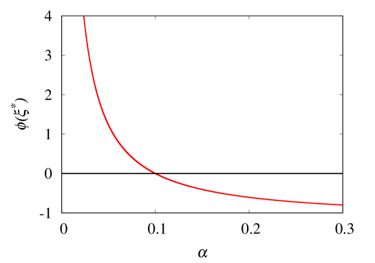
Figure 4: $\phi(\xi^{*})$ vs $\alpha$ for $\alpha_{1}=1$, $\lambda_{1}=0.1$, $\alpha_{2}=-\alpha$, $\lambda_{2}=1$.

Figure 5 depicts the behavior of $\xi_{+}$ and $\xi_{-}$ vs $\alpha$ in the same conditions.

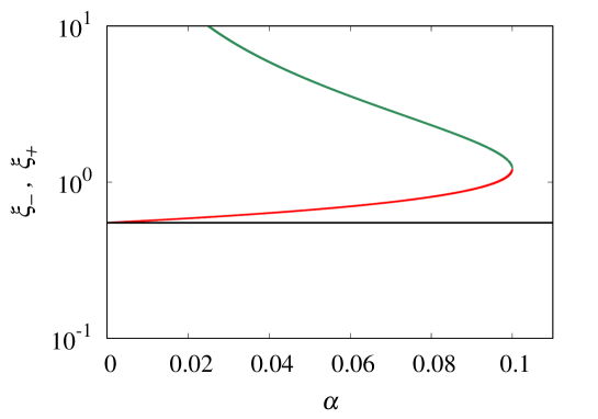
Figure 5: $\xi_{+}$ (upper curve) and $\xi_{-}$ (lower curve) vs $\alpha$, for $\alpha_{1}=1$, $\lambda_{1}=0.1$, $\alpha_{2}=-\alpha$, $\lambda_{2}=1$. The horizontal line corresponds to the value of $\xi_{\rm min}$.

Given $\alpha<\alpha_{\rm nc}$, any value of $\xi\in(\xi_{-},\xi_{+})$ produces a stochastic realization of the system at equilibrium, satisfying either FD1k or FD2k in its strong form.

For $\alpha<\alpha_{nc}$, any value of $\xi$ in the interval $(\xi_{-},\xi_{+})$ produces an equivalent model of the equilibrium behavior. To this end, we have to show that all these realizations for $\xi\in(\xi_{-},\xi_{+})$ give rise to one and the same autocorrelation function of the resulting stochastic force at equilibrium (i.e. in the long-term). To avoid misunderstandings, it is useful to remain that we are here considering a nondimensional formulation with $m=1$, and $\langle v^{2}\rangle_{\rm eq}=1$, and thus the FD2k result in the strong form corresponds to $C_{RR}(t)=h(t)$. To verify this property consider the expression for the stochastic force $R(t)$. From eq. (40) we have

$$R(t)=\sum_{i=1}^{2}a_{i}\,z_{i,0}\,e^{\-\lambda_{i}\,t}+\sqrt{2}\sum_{i=1}^{2}a_{i}\sum_{h=1}^{2}\,\beta_{i,h}\,e^{-\lambda_{i}t}*\xi_{h}(t)=2\sum_{i=1}^{2}a_{i}\sum_{h=1}^{2}\beta_{i,h}\,r_{i,h}(t)$$ (56)

where we have set

$$r_{i,h}(t)=e^{-\lambda_{i}t}*\xi_{h}(t)\,,\qquad i,h=1,2$$ (57)

In the long-term (equilibrium), the first term at the r.h.s. of eq. (56) decays exponentially to zero, so that

$$C_{RR}(t)=\langle R(t)\,R(0)\rangle_{\rm eq}=2\sum_{i=1}^{2}a_{i}\sum_{h=1}^{2}\beta_{i,h}\sum_{j=1}^{2}a_{j}\sum_{k=1}^{2}\beta_{j,k}\,\langle r_{i,h}(t)\,r_{j,k}(0)\rangle_{\rm eq}$$ (58)

where

$$\langle r_{i,h}(t)\,r_{j,k}(0)\rangle_{\rm eq}=\lim_{\tau\rightarrow\infty}\langle r_{i,h}(t+\tau)\,r_{j,k}(\tau)\rangle$$ (59)

The latter expression can be easily calculated by quadraturae, enforcing the property $\xi_{h}(t)\,\xi_{k}(\tau)=\delta_{h,k}\,\delta(t-\tau)$, and this yields

$$\langle r_{i,h}(t)\,r_{j,k}(0)\rangle_{\rm eq}=\frac{e^{\lambda_{i}\,t}}{\lambda_{i}+\lambda_{j}}\,\delta_{h,k}$$ (60)

Inserting the latter expression into eq. (58), we finally arrive to

$$C_{RR}(t) = 2\sum_{i=1}^{2}a_{i}\sum_{h=1}^{2}\beta_{i,h}\sum_{j=1}^{2}a_{j}\sum_{k=1}^{2}\beta_{j,k}\,\frac{e^{\lambda_{i}\,t}}{\lambda_{i}+\lambda_{j}}\,\delta_{h,k}=2\sum_{i=1}^{2}a_{i}\sum_{j=1}^{2}\frac{a_{j}}{\lambda_{i}+\lambda_{j}}\,e^{-\lambda_{i}\,t}\sum_{h=1}^{2}\beta_{i,h}\,\beta_{j,h}$$ (61)

$$= \sum_{i=1}^{2}a_{i}\,e^{-\lambda_{i}\,t}\,\left[\sum_{j=1}^{1}2\,a_{j}\frac{S_{i,j}}{\lambda_{i}+\lambda_{i}}\right]$$

The expression within square parentheses at the r.h.s. of eq. (61) is identically equal to one for $i=1,2$ because of eqs. (48), and thus eq. (61) simply becomes

$$C_{RR}(t)=\sum_{i=1}^{2}a_{i}\,e^{-\lambda_{i}\,t}=h(t)$$ (62)

which proves that for any plausible choice of $\xi$, all the stochastic realizations are equivalent and satisfy FD2k.

Appendix IV - Linear response theory: exponential divergence outside ${\mathcal{D}}_{\rm ds}$ - Consider the case of “well-behaved kernels” $h(t)$ possessing real and negative poles. In this case, the classical theory predicts a bounded response in the presence of a periodically forced term kubo2

$$\frac{dv(t)}{dt}=-\int_{0}^{t}h(t-\tau)\,v(\tau)\,d\tau+F(t;\omega)$$ (63)

where $F(t;\omega)$ is a sinusoidal perturbation of frequency $\omega$, say $F(t;\omega)=F_{0}\,e^{\mathrm{i}\,\omega\,t}$, i.e., $v(t;\omega)=\mu(\omega)\,F_{0}\,e^{\mathrm{i}\,\omega\,t}$, controlled by the mobility function $\mu(\omega)$ kubo2 ,

$$\mu(\omega)=\frac{1}{\mathrm{i}\,\omega+h[\omega]}$$ (64)

where $h[\omega]=\widehat{h}(\mathrm{i}\,\omega)$ is the Laplace-Fourier transform of $h(t)$. This is not true if the GLE is not dissipatively stable, for which the dynamics diverges exponentially in time in the presence of generic sinusoidal perturbations, with an exponent controlled by the real part of dominant eigenvalue, i.e. of the eigenvalue possessing the largest real part.

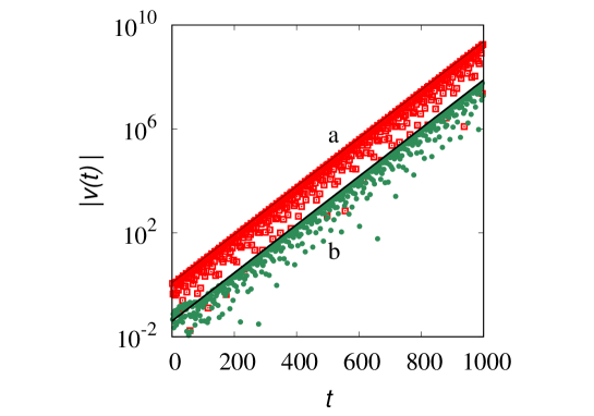
Figure 6: $|v(t)|$ vs $t$ for sinusoidal forcings: (a): $F(t,;\omega)=\cos(\omega\,t)$; (b): $F(t;\omega)=\sin(\omega\,t)$ at $\omega=0.03$.

To show this, consider the kernel $h(t)$ given by eq. (39) at $\alpha=0.3$. In this case, the eigenvalues of the matrix ${\bf A}$ associated with $h(t)$ are: $\mu_{1,2}=\mu_{u}\pm\mathrm{i}\,\omega_{u}$, with $\mu_{u}\simeq 2.137\,\times 10^{-2}$, $\omega_{u}\simeq 0.921$, and $\mu_{3}=\mu_{s}\simeq-1.14274$, corresponding to a couple of unstable complex conjugate eigenvalues and a stable real one. The response to any perturbation can be easily estimated in the Laplace domain (assuming $v(t=0)=0$),

$$\widehat{v}(s) = \frac{1}{s+\widehat{h}(s)}\,\widehat{F}(s;\omega)$$

$$= \frac{(s+\lambda_{1})\,(s+\lambda_{2})}{s\,(s+\lambda_{1})\,(s+\lambda_{2})+a_{1}\,(s+\lambda_{2})+a_{2}\,(s+\lambda_{1})}\,\widehat{F}(s;\omega)$$

$$= \left[\frac{A+B\,s}{(s-\mu_{u})^{2}+\omega_{u}^{2}}+\frac{C}{s-\mu_{s}}\right]\,\widehat{F}(s;\omega)$$

where $A,\,B\,,C$ can be easily calculated from the expansion in partial fractions. For large $t$, solely the first term at the r.h.s. of eq. (Dynamic fluctuation-dissipation theory for Generalized Langevin Equations: constructive constraints, stability and realizability) is relevant and it corresponds to a $v(t)$ exponentially growing in time with the exponent $\mu_{\rm max}=\mu_{u}$ with a prefactor that depends on the frequency $\omega$. Specifically

$$v(t)=\mu_{c}^{(e)}(\omega)\,F_{0}\,e^{\mu_{u}\,t}\,\cos(\omega_{u}\,t+\varphi_{c})$$ (66)

if $F(t;\omega)=F_{0}\,\cos(\omega\,t)$, and

$$v(t)=\mu_{s}^{(e)}(\omega)\,F_{0}\,e^{\mu_{u}\,t}\,\cos(\omega_{u}\,t+\varphi_{s})$$ (67)

if $F(t;\omega)=F_{0}\,\sin(\omega\,t)$, where $\mu_{c}^{(e)}(\omega)$ and $\mu_{s}^{(e)}(\omega)$, referred to as the “exponential mobilities” can be obtained analytically from eq. (Dynamic fluctuation-dissipation theory for Generalized Langevin Equations: constructive constraints, stability and realizability) in the two cases considered, and $\varphi_{c}$ and $\varphi_{s}$ are the phase-shifts. Figure 6 shows some examples of this exponential behavior, while the behavior of the exponential mobilities $\mu_{c}^{(e)}(\omega)$ and $\mu_{s}^{(c)}(\omega)$ is reported in the main text. For dissipatively unstable systems, apart from the exponential divergence with time, the frequency of the oscillations is locked to $\omega_{u}$, independently of $\omega$, marking the difference with respect to the dissipatively stable case.

References

(1) R. Kubo, Rep. Prog. Phys. 29 255 (1966).
(2) R. Kubo, M. Toda and N. Hashitsune, Statistical Physics II Nonequilibrium
Statistical Mechanics (Springer-Verlag, Berlin, 1991).
(3) A. Widom, Phys. Rev. A 3 1394 (1971).
(4) U. Marini Bettolo Marconi, A. Puglisi, L. Rondoni and A. Vulpiani, Phys. Rep. 461 111 (2008).
(5) O. Darrigol, Eur. Phys. J. H 48 10 (2023).
(6) A. Caspi, R. Granek, and M. Elbaum, Phys. Rev. Lett. 85
5655 (2000).
(7) C. Wilhelm, Phys. Rev. Lett. 101 028101 (2008).
(8) P. Langevin,
C. R. Acad. Sci. (Paris) 146 530 (1908); english
translation in Am. J. Phys. 65 1079 (1997).
(9) B U Felderhof, J. Phys. A 11 921 (1978).
(10) V. Balakrishnan, Pramana 12 301 (1979).
(11) R. Zwanzig,
Phys. Rev. 124 983 (1961).
(12) J. Tothova , G. Vasziova, L. Glod,
and V. Lisy, Eur. J. Phys. 32 645 (2011).
(13) H.-Y. Yu, D. M. Eckmann, P. S. Ayyaswamy, and R. Radhakrishnan,
Phys. Rev. E 91 052303 (2015).
(14) S. A. McKinley and H. D. Nguyen, SIAM J. Math. Anal. 50 5119 (2018).
(15) Y. Hino and S. Murakami, J. Diff. Eq. 89 121 (1991).
(16) Y. Hino and S. Murakami, Funkcialaj Ekvacioj 48 367 (2005).
(17) S. R. De Groot and P. Mazur Non-Equilibrium
Thermodynamics (Dover Publ., Mineola USA, 1984).
(18) R. Huang, I. Chavez, K. M. Taute, B. Lukic, S. Jeney,
M. G. Raizen and E. L. Florin,
Nature Phys. 7
576 (2011).
(19) T. Franosch, M. Grimm, M. Belushkin,
F. M. Mor, G. Foffi, L. Forró and S. Jeney,
Nature 478 85 (2011).
(20) T. Li and M. G. Raizen, Ann. Phys. (Berlin)
525 281 (2013).
(21) S. Kheifets, A. Simha, K. Melin, T. Li and M. G. Raizen,
Science 343 1493 (2014).
(22) M. Grimm, S. Jeney and T. Franosch, Soft Matter 7, 2076 (2011).
(23) G. Procopio and M. Giona,
Fluids 8 84 (2023).
(24) C. W. Makosko, Rheology - Principles, Measurements, and Applications
(Wiley-VCH, New York, 1994).
(25) J. D. Ferry, Viscoelastic Properties of Polymers (J. Wiley & Sons, New York, 1970).
(26) R. K. Miller, J. Diff. Eq. 10 485 (1971).
(27) S. I. Grossman and R. K. Miller, J. Diff. Eq. 13 551 (1973).
(28) J.-D. Bao, P Hänggi and Y.-Z. Zhuo, Phys. Rev. E 72 061107 (2005).
(29)J.-D. Bao, Eur. Phys. J. B 93 184 (2020).
(30) A. V. Plyukhin, Phys. Rev. E 83 062102 (2011).
(31) F. Ishikawa and S. Todo, Phys. Rev. E 98 062140 (2018).
(32) A. V. Plyukhin, Phys. Rev. E 105 014121 (2022).
(33) G. Procopio, C. Pezzotti and M. Giona,
On the ergodicity breaking in well-behaved Generalized Langevin Equations,
in preparation (2024).
(34) N. G. van Kampen, Stochastic Processes in Physics and Chemistry
(Elsevier, Amsterdam, 2007).
(35) I. Goychuk
Adv. Chem. Phys. 150, 187 (2012).
(36) L. Stella, C. D. Lorenz and L. Kantorovich,
Phys. Rev. B 69, 123303 (2014).
(37) H. Ness, L. Stella, C.D. Lorenz and L. Kantorovich,
Phys. Rev. B 91, 014301 (2015).