Simulating conditioned diffusions on manifolds

Abstract.

To date, most methods for simulating conditioned diffusions are limited to the Euclidean setting. The conditioned process can be constructed using a change of measure known as Doob’s $h$-transform. The specific type of conditioning depends on a function $h$ which is typically unknown in closed form. To resolve this, we extend the notion of guided processes to a manifold $M$, where one replaces $h$ by a function based on the heat kernel on $M$. We consider the case of a Brownian motion with drift, constructed using the frame bundle of $M$, conditioned to hit a point $x_{T}$ at time $T$. We prove equivalence of the laws of the conditioned process and the guided process with a tractable Radon-Nikodym derivative. Subsequently, we show how one can obtain guided processes on any manifold $N$ that is diffeomorphic to $M$ without assuming knowledge of the heat kernel on $N$. We illustrate our results with numerical simulations and an example of parameter estimation where a diffusion process on the torus is observed discretely in time.

Keywords: bridge simulation, Doob’s $h$-transform, geometric statistics, guided processes, Riemannian manifolds

AMS subject classification: 62R30, 60J60, 60J25

1. Introduction

Let $M$ be a compact $d$-dimensional Riemannian manifold and let $V$ be a smooth vector field on $M$. Denote by $\tilde{V}$ the horizontal lift of $V$ to the frame bundle ${\mathrm{F}M}$ of $M$ and consider the Stratonovich stochastic differential equation (SDE)

$$\,\mathrm{d}U_{t}=\tilde{V}(U_{t})\,\mathrm{d}t+H_{i}(U_{t})\circ\,\mathrm{d}W_{t}^{i},\qquad U_{0}=u_{0}.$$ (1.1)

where $H_{1},\dots,H_{d}$ are the canonical horizontal vector fields, $u_{0}$ an orthonormal frame, and $W$ an ${\mathbb{R}}^{d}$-valued Brownian motion. We use Einstein’s summation convention to sum over all indices that appear in both sub- and superscript. The aim of this paper is to construct a method for simulation of the process $X=\pi(U)$, started at $x_{0}=\pi(u_{0})$ and conditioned on hitting some $x_{T}\in M$ at time $T>0$, where $\pi$ denotes the projection from ${\mathrm{F}M}$ to $M$. Such a process is often called a pinned-down diffusion or diffusion bridge. For readers unfamiliar with SDEs on manifolds, we provide background and references in Section 2.

1.1. Motivation and applications

A diffusion defined by a stochastic differential equation provides a flexible way to model continuous-time stochastic processes. Whereas the process is described in continuous-time, observations are virtually always discrete in time, possibly irregularly spaced. Transition densities are rarely known in closed form, complicating likelihood-based inference for parameters in either the drift- or diffusion coefficients of the SDE. To resolve this, data-augmentation algorithms have been proposed where the latent process in between observation time is imputed. For diffusions that take values in a linear space, numerous works over the past two decades have shown how to deal with this problem (e.g. Beskos et al., (2006a); Golightly & Wilkinson, (2010); Papaspiliopoulos et al., (2013); Mider et al., (2021)). The corresponding problem where the process takes values in a manifold has received considerably less attention, despite its importance in various application settings. Examples include evolving particles on a sphere, evolution of positive-definite matrices and evolution of compositional data. From a more holistic point of view, our work potentially comprises an important step for statistical inference in state space models on manifolds (Manton, (2013), Section III).

Applications of conditioned manifold processes also arise in shape analysis e.g. Sommer et al., (2017); Arnaudon et al., (2022) and more generally in geometric statistics, e.g. Jensen et al., (2022), which focuses on Lie groups and homogeneous spaces. See Sommer, (2020) for a general overview. Bridges can be applied to model shape changes caused by progressing diseases as observed in medical imaging, or to model changes of animal morphometry during evolution and subsequently used for analyzing phylogenetic relationships between species.

1.2. Related work

Bridge simulation on Euclidean spaces has been treated extensively in the literature. See for instance Durham & Gallant, (2002); Stuart et al., (2004); Beskos et al., (2006b, 2008); Hairer et al., (2009); Lin et al., (2010); Bladt et al., (2016); Whitaker et al., (2017); Bierkens et al., (2021) and references therein. It is known that the conditioned process satisfies a stochastic differential equation itself, where a guiding term that depends on the transition density of the process is superimposed on the drift of the unconditioned process. Unfortunately, transition densities are only explicit in very special cases. One class of methods to construct conditioned processes consists of approximating the true guiding term by a tractable substitute. The resulting processes are called guided proposals, guided processes or twisted processes. By explicit computation of the likelihood ratio between the true bridge and the approximating guided process any discrepancy can be corrected for in (sequential) importance sampling or Markov chain Monte Carlo methods. The approach taken in this paper falls into this class.

Early instances of this approach are Clark, (1990) and Delyon & Hu, (2006) where the guiding term matches the drift of a Brownian bridge. A different, though related, approach is construct a guiding term based on $\nabla_{x}\log\tilde{p}(t,x;T,x_{T})$, where $\tilde{p}$ is the transition density of a diffusion for which it is known in closed form (see Schauer et al., (2017) and Bierkens et al., (2020)). A linear process is a prime example of such diffusions.

There is extensive literature on manifold stochastic processes, their construction and bridges, see e.g. Emery, (1989); Hsu, (2002). The construction of conditioned manifold processes is the subject of Baudoin, (2004). Direct adaptation of bridge simulation methods devised for Euclidean space by embedding the manifold in $\mathbb{R}^{d}$ easily run into difficulties as the diffusivity matrix becomes singular, the drift unbounded and the numerical scheme has to be particularly adapted to ensure that the process in the embedding space stays on the manifold. In the geometric setting, the approach of Delyon & Hu, (2006) is generalized to manifolds in Jensen et al., (2019); Jensen & Sommer, (2021); Bui et al., (2023). The drift here comes from the gradient of the square distance to the target, mimicking the drift of the Euclidean drift approximation. An important complication with this approach is handling the discontinuity of the gradient at the cut locus of the target point. This is introducing unnecessary complexities because the true guiding term is often smooth, and the scheme effectively approximates the smooth true transition density with a discontinuous guiding term which is harder to control, both numerically and analytically. With the approach in the presented paper, we exactly achieve smooth guiding terms in accordance with the true transition density and we avoid the cut locus issues. In addition, to ensure that the guided process in fact hits the conditioning point, Jensen et al., (2019); Jensen & Sommer, (2021) impose a Lyapunov condition on the radial process. Verifying this assumption for a specified vector field $V$ is difficult. The approach taken in this paper avoids this condition altogether. Bui et al., (2023) don’t formally prove absolute continuity though carefully assess validity of their approach by extensive numerical simulation.

1.3. Approach and main results

We extend the approach of simulating Euclidean diffusion bridges from Schauer et al., (2017) to manifolds. If $X$ is a Euclidean SDE with drift $b$ and diffusion coefficient $\sigma$, an SDE for the conditioned process $X^{h}$ (with law ${\mathbb{P}}^{h}$) is obtained by superimposing the SDE for $X$ with the term $\sigma\sigma^{\prime}\nabla\log h\,\mathrm{d}t$, where $h$ is the intractable transition density of $X$. It is thus impossible to directly simulate $X^{h}$. Instead, $X$ is approximated by an ”auxiliary” linear process $\tilde{X}$ with known closed-form transition density $g$, and the SDE for $X$ is superimposed with a term $\sigma\sigma^{\prime}\nabla\log g\,\mathrm{d}t$ resulting in a guided process $X^{g}$ (with law ${\mathbb{P}}^{g}$). This process is not equal to $X^{h}$ in law, but the likelihood ratio is computable and the resulting scheme allows expectations $\mathbb{E}f(X^{h})$ over the conditioned process to be evaluated. As sketched in Figure 1, the approach presented in this paper is a geometric equivalent of this construction: We cannot simulate the conditioned process $X^{h}$ for a process $X$ on a manifold $N$ because of intractability of the transition density. Instead, if $N$ is diffeomorphic to a comparison manifold $M$ with closed form heat kernel $g$, we map this guiding term from $M$ to $N$ to give a guided process $X^{g}$ on $N$, again with computable likelihood ratio allowing evaluation of $\mathbb{E}f(X^{h})$. The ”auxiliary” process in this case is thus a Brownian motion on $N$. Figure 1 sketches a comparison between this approach and Schauer et al., (2017).

(a) Euclidean: $X$ is conditioned using $h$ to obtain $X^{h}$. Since $h$ is intractable, we derive $g$ from an auxiliary process $\tilde{X}$, and use it to define $X^{g}$. The tractable likelihood ratio $\,\mathrm{d}{\mathbb{P}}^{h}/\,\mathrm{d}{\mathbb{P}}^{g}$ allows for evaluation of ${\mathbb{E}}f(X^{h})$.

(b) Geometric: $X$ is conditioned using $h$ to obtain $X^{h}$. Since $h$ is intractable, we derive $g$ from an auxiliary process $\tilde{Y}$, a Brownian motion on a comparison manifold $M$, and use it to define $X^{g}$. The tractable likelihood ratio $\,\mathrm{d}{\mathbb{P}}^{h}/\,\mathrm{d}{\mathbb{P}}^{g}$ allows for evaluation of ${\mathbb{E}}f(X^{h})$.

Figure 1. Diagrams sketching the approach for conditioning diffusion processes.

Our approach is applicable for compact manifolds $N$ diffeomorphic to a manifold on which the heat kernel is known in closed form. This includes many cases such as Euclidean spaces with non-standard Riemannian metrics, spheres and ellipsoids, hyperbolic spaces, and tori with different metrics (flat, embedded).

The main results are 3.4 and 4.2. We illustrate our results in a statistical application where we estimate a parameter in the vector field $V$ from discrete-time observations of the process. Compared to earlier work this has the following advantages: (i) the guiding term is smooth and thereby avoids analytical and numerical issues caused by discontinuities at the cut locus of the target; as a consequence of this, the numerics for computing the likelihood ratio between true conditioned process and guided process is easier as we avoid computing local times; (ii) no Lyapunov condition (that is hard to verify) needs to be imposed.

1.4. Outline

In Section 2, we give some background on SDEs on manifolds. All main results of the paper are stated in Sections 3 and 4. We detail the approach taken in this paper in Section 3 in the specific case that $\Phi$ is the identity. In Section 4 we extend this result to a case where $\Phi$ is a diffeomorphism between manifolds $M$ and $N$ and the heat kernel is known on $N$. In Section 5, we illustrate the usefulness of our results in numerical simulations of diffusion bridges and a parameter estimation problem for a discretely observed diffusion process on the torus. In Section 6, we show how our approach can be extended to other types of conditionings at a fixed future time. Finally, all proofs are gathered in Section 7.

2. Background on SDEs on manifolds

We consider SDEs on manifolds as developments of ${\mathbb{R}}^{d}$-valued semimartingales. We sketch the main concepts here. For a detailed description, we refer to Hsu, (2002); Emery, (1989). With $M$ a $d$-dimensional Riemannian manifold and $x\in M$, the tangent space $T_{x}M$ to $M$ at $x$ is a $d$-dimensional vector space. A frame $u$ is a basis for $T_{x}M$, equivalently an isomorphism $u\colon{\mathbb{R}}^{d}\to T_{x}M$. The collection of all frames at $x$ is denoted by $\mathrm{F}_{x}M$ and the vector bundle with fibers $\mathrm{F}_{x}M$ is called the frame bundle $\mathrm{F}M$. The canonical projection, which maps a frame $u$ at $x$ to $x$, is denoted by $\pi\colon{\mathrm{F}M}\to M$.
${\mathrm{F}M}$ is a manifold itself of dimension $d+d^{2}$. It has a submanifold ${\mathrm{O}M}$ consisting of orthonormal frames. A derivative of a curve in ${\mathrm{F}M}$ can be decomposed in a horizontal part, which corresponds to infinitesimal parallel translation of the basis along the projection onto $M$, and a vertical part, which is derivative of a curve for which the projection stays constant but the frame changes over time. Therefore, for $u\in{\mathrm{F}M}$, $T_{u}{\mathrm{F}M}$ can be written as a direct sum $T_{u}{\mathrm{F}M}=\mathcal{H}_{u}{\mathrm{F}M}\oplus\mathcal{V}_{u}{\mathrm{F}M}$ of the horizontal and vertical subspaces, respectively. The horizontal subspace is a vector space of dimension $d$ with a basis $H_{1}(u),\dots,H_{d}(u)$ consisting of the globally defined horizontal fields $H_{1},\ldots,H_{d}$ that in local coordinates at $u=(x^{i},\nu^{i}_{j})$ are given by

$$H_{i}(u)=\nu^{j}_{i}\frac{\partial}{\partial x^{j}}-\nu^{j}_{i}\nu^{l}_{m}\Gamma^{k}_{jl}\frac{\partial}{\partial\nu^{k}_{m}}$$

An ${\mathbb{R}}^{d}$-valued semimartingale $Z$ can be uniquely mapped to a horizontal process $U$ via the Stratonovich SDE

$$\,\mathrm{d}U_{t}=H_{i}(U_{t})\circ\,\mathrm{d}Z_{t}^{i}.$$

The process $U$ is called the development of $Z$ and the projection $\pi(U)$ is the development of $Z$ on $M$. The development is reversible in the sense that, for a horizontal semimartingale $U$, a unique ${\mathbb{R}}^{d}$-valued semimartingale $Z$ exists so that $U$ is the development of $Z$. This $Z$ is denoted the anti-development of $U$. It can be shown that if $W$ is an ${\mathbb{R}}^{d}$-valued Brownian motion and $U_{0}=u_{0}\in{\mathrm{O}M}$, then $\pi(U)$ is Brownian motion in $M$.

If $X$ is a semimartingale on $M$, a horizontal semimartingale $U$ such that $\pi(U)=X$ is denoted a horizontal lift of $X$. For a function $f\colon M\to{\mathbb{R}}$, we denote by $\tilde{f}\colon{\mathrm{F}M}\to{\mathbb{R}}$ the function $f\circ\pi$. For $u\in{\mathrm{F}M}$, a vector $V\in T_{\pi(u)}M$ can be uniquely lifted to $\mathcal{H}_{u}{\mathrm{F}M}$ using the horizontal vector fields. This vector is then denoted by $\tilde{V}$. In particular, for a function $f\colon M\to{\mathbb{R}}$, we denote the lift of $\nabla f$ by $\nabla^{H}\tilde{f}=\left\{H_{i}\tilde{f},\dots,H_{d}\tilde{f}\right\}$ and refer to it as the horizontal gradient.

3. Guided processes on manifolds

In this section, we introduce guided processes taking values on a manifold $M$. We here assume that on $M$ a closed form expression for the heat kernel, possibly a series expansion, is known. In Section 4, we treat the more general situation of a manifold $N$ being diffeomorphic to $M$.

Throughout, we assume that we are working on a probability space $(\Omega,\mathcal{F},{\mathbb{P}})$. Let $X$ be an $M$-valued Markov process with infinitesimal generator ${\mathfrak{L}}$ and denote ${\mathfrak{A}}=\partial_{t}+{\mathfrak{L}}$. Let $\mathcal{F}_{t}=\sigma\left(\left\{X_{s}:s\leq t\right\}\right)$ be the natural filtration induced by $X$ and denote the restriction of ${\mathbb{P}}$ to $\mathcal{F}_{t}$ by ${\mathbb{P}}_{t}=\left.{\mathbb{P}}\right\rvert_{\mathcal{F}_{t}}$. We denote by $\mathcal{M}(M)$ the space of measurable functions from $[0,T)\times M$ to ${\mathbb{R}}$. Define $\{E_{t}^{f}(X)\colon t\in[0,T)\}$ by

$$E_{t}^{f}(X)=\frac{f(t,X_{t})}{f(0,X_{0})}\exp\left(-\int_{0}^{t}\frac{{\mathfrak{A}}f(s,X_{s})}{f(s,X_{s})}\,\mathrm{d}s\right)$$ (3.1)

and let

$$\mathcal{H}=\left\{f\in\mathcal{M}(M)\>\colon f>0\text{ and }\{E_{t}^{f}(X)\,\colon t\in[0,T)\}\text{ is a martingale}\right\}.$$

For $f\in\mathcal{H}$, the change of measure

$$\frac{\,\mathrm{d}{\mathbb{P}}_{t}^{f}}{\,\mathrm{d}{\mathbb{P}}_{t}}=E_{t}^{f}(X),\quad t\in[0,T)$$ (3.2)

defines a family of probability measures $\left\{{\mathbb{P}}^{f}_{t},\,t\in[0,T)\right\}$. Since (3.2) uniquely determines a family of consistent finite dimensional distributions, Kolmogorov’s extension theorem implies that there exists a unique probability measure ${\mathbb{P}}^{f}$ such that, for all $t$, $\left.{\mathbb{P}}^{f}\right\rvert_{\mathcal{F}_{t}}={\mathbb{P}}_{t}^{f}$. We refer to the measure ${\mathbb{P}}^{f}$ as the measure induced by $f$. Expectations with respect to ${\mathbb{P}}^{f}$ are denoted by ${\mathbb{E}}^{f}$.

Specific choices of $f$ correspond to conditioning the process $X$ on certain events. Harmonic functions $h\in\mathcal{H}$ with the additional property $\mathfrak{A}h=0$ play an important role. For such $h$, $\mathbb{P}^{h}$ is called Doob’s $h$-transform of $\mathbb{P}$.

We concentrate on conditioning the process on the event $\{X_{T}=x_{T}\}$ with $x_{T}\in M$, postponing other types of conditioning to Section 6. We assume the transition kernel of $X$ admits a density $p$ with respect to the volume measure $\,\mathrm{d}\mathrm{Vol}_{M}(x)$ on $M$, i.e. ${\mathbb{P}}\left(X_{t}\in A\mid X_{s}=x\right)=\int_{A}p(s,x;t,y)\,\mathrm{d}\mathrm{Vol}_{M}(y)$ for $s\leq t$, $A\subseteq M$ measurable and $x\in M$. Then, $h(t,x)=p(s,t;T,x_{T})$ satisfies $\mathfrak{A}h=0$ and induces the process $\left(X\mid X_{T}=x_{T}\right)$ (see e.g Theorem 5.4.1 of Hsu, (2002)).

Since transition densities for diffusions on manifolds are rarely known in closed form, we use the results of Corstanje et al., (2023) to work around not knowing $h$ by replacing it with a tractable substitute, which we will denote by $g$. This gives the following result.

Proposition 3.1.

Suppose $h\in\mathcal{H}$ is such that ${\mathfrak{A}}h=0$ and let $g\in\mathcal{H}$. Then, for $t<T$, ${\mathbb{P}}_{t}^{h}\ll{\mathbb{P}}_{t}^{g}$ with

$$\frac{\,\mathrm{d}{\mathbb{P}}^{h}_{t}}{\,\mathrm{d}{\mathbb{P}}^{g}_{t}}=\frac{E_{t}^{h}(X)}{E_{t}^{g}(X)}=\frac{g(0,X_{0})}{h(0,X_{0})}\frac{h(t,X_{t})}{g(t,X_{t})}\exp\left(\int_{0}^{t}\frac{{\mathfrak{A}}g(s,X_{s})}{g(s,X_{s})}\,\mathrm{d}s\right).$$ (3.3)

Under ${\mathbb{P}}^{g}$, the horizontal lift of $X$ satisfies the SDE

$$\,\mathrm{d}U_{t}=\tilde{V}(U_{t})\,\mathrm{d}t+\nabla^{H}\log\tilde{g}(t,U_{t})\,\mathrm{d}t+H_{i}(U_{t})\circ\,\mathrm{d}W_{t}^{i},$$ (3.4)

where we again used Einsteins summation convention. Alternatively, one could also write $U$ under ${\mathbb{P}}^{h}$ as the stochastic development of an ${\mathbb{R}}^{d}$-valued process through

$$\,\mathrm{d}U_{t}=H_{i}(U_{t})\circ\left[U_{t}^{-1}\tilde{V}(U_{t})\,\mathrm{d}t+U_{t}^{-1}\nabla^{H}\log\tilde{g}(t,U_{t})\,\mathrm{d}t+\,\mathrm{d}W_{t}^{i}\right]$$

Proof.

Equation 3.3 follows directly from (3.2). The SDE for $U$ follows from its extended generator, which can be obtained from A.1. ∎

We call the process $X$ under $\mathbb{P}^{g}_{t}$ the guided process, as an appropriate choice of $g$ should guide the process to the event we wish to condition on. As an intermediate result, we obtain a Feynman-Kac type formula for the intractable function $h$ in terms of a process that is amenable to stochastic simulation.

Corollary 3.2.

Let $h(t,x)=\int p(t,x;T,y)q(y)\,\mathrm{d}\mathrm{Vol}_{M}(y)$ such that $\mathbb{P}^{h}\ll\mathbb{P}$. Then $h$ is characterised in terms of the guided process by

$${h(t,x)}=\mathbb{E}^{g}\,\left[\left.{g(t,x)}\frac{q(X_{T})}{g(T,X_{T})}\exp\left(\int_{t}^{T}\frac{{\mathfrak{A}}g(s,X_{s})}{g(s,X_{s})}\,\mathrm{d}s\right)\right|X_{t}=x\right].$$ (3.5)

Consider $U$ as defined by (1.1). The process $X=\pi(U)$ has extended generator ${\mathfrak{A}}$ on the domain ${\mathfrak{D}}({\mathfrak{A}})=\mathcal{C}^{1,2}([0,T)\times M)$ with

$${\mathfrak{A}}f=\partial_{t}f+{V}{f}+\frac{1}{2}\Delta f$$

for $f\in{\mathfrak{D}}({\mathfrak{A}})$ and where $\Delta$ denotes the Laplace-Beltrami operator on $M$.

3.1. Guiding induced by the heat kernel

Let $\kappa$ be the minimal heat kernel on $M$. That is $\kappa\colon[0,T]\times M\times M\to{\mathbb{R}}$ is the unique minimal solution to the partial differential equation

$$\partial_{t}\kappa(t,x,y)=\frac{1}{2}\Delta_{x}\kappa(t,x,y)$$ (3.6)

satisfying $\int_{M}\kappa(t,x,y)\,\mathrm{d}\mathrm{Vol}_{M}(y)=1$. Here $\Delta_{x}$ denotes the Laplace-Beltrami operator applied to the $x$-argument. Notice that, $\kappa$ exists on compact manifolds, as they are stochastically complete. We define the guiding function

$$g(t,x)=\kappa(T-t,x,x_{T})$$ (3.7)

By Proposition 4.1.6 in Hsu, (2002), $g$ is the transition density function of a Brownian motion on $M$. We require $X$ to have a transition density $p$ as well. The relationship between $p$ and the heat kernel is described in 3.3.

Proposition 3.3.

Let $M$ be a compact Riemannian manifold. Then $X$ admits a transition density $p$ with respect to the volume measure for which positive constants $\gamma_{1},\gamma_{2},\gamma_{3}$ exists such that for all $s\leq t$ and $x,y\in M$,

$$p(s,x;t,y)\leq\gamma_{1}\kappa(\gamma_{2}(t-s),x,y)e^{-\gamma_{3}(t-s)}$$

Proof.

It follows from Sturm, (1993) that this assumption is satisfied if $M$ has Ricci curvature bounded from below, which is the case for compact manifolds. ∎

The following theorem gives sufficient conditions for equivalence of the measures ${\mathbb{P}}^{h}_{T}$ and ${\mathbb{P}}^{g}_{T}$. It is key to our numerical simulation results presented in Section 5.

Theorem 3.4.

Assume $M$ is a compact manifold and $V$ is a smooth vector field on $M$. Then ${\mathbb{P}}_{T}^{h}\sim{\mathbb{P}}_{T}^{g}$ with

$$\frac{\,\mathrm{d}{\mathbb{P}}_{T}^{h}}{\,\mathrm{d}{\mathbb{P}}^{g}_{T}}=\frac{g(0,x_{0})}{h(0,x_{0})}\Psi_{T,g}(X),$$ (3.8)

where

$$\Psi_{T,g}(X)=\exp\left(\int_{0}^{T}V\left(\log g\right)(s,X_{s})\,\mathrm{d}s\right).$$ (3.9)

The proof is deferred to Section 7.3. Upon integration of (3.8) with respect to ${\mathbb{P}}^{g}$, we obtain an expression for the transition density as

$$p(0,x_{0};T,x_{T})=g(0,x_{0}){\mathbb{E}}^{g}\Psi_{T,g}(X).$$ (3.10)

4. Guiding with comparison manifolds

The assumption that the heat kernel is known in closed form is restrictive. Suppose $N$ is a manifold for which there exists a diffeomorphism $\Phi\colon M\to N$. Assuming that the heat kernel on $M$ is tractable, we will construct a guided process on $N$ by mapping the guiding term from $M$ to $N$.

Let $X=\pi(U)$ be an $M$-valued stochastic process, with $U$ defined by (1.1). 3.4 shows how samples from $X$ under ${\mathbb{P}}^{h}$ can be weighted to obtain samples from ${\mathbb{P}}^{g}$. Denote the process $X$ under ${\mathbb{P}}^{h}$ by $X^{h}$. Define the $N$-valued process $Y$ by $Y_{t}=\Phi(X_{t})$ and denote the law of $Y$ by ${\mathbb{Q}}$. Define $\Phi_{*}h\in\mathcal{M}(N)$ by $(\Phi_{*}h)(t,y)=h(t,\Phi^{-1}(y))$.

The theorem below shows that first $h$-transforming $X$ and then mapping it to $N$ through $\Phi$ results in the same process (in law) as $h$-transforming the process $\Phi(X)$ with $\Phi_{*}h$. In other words, the diagram in Figure 2 commutes.

Theorem 4.1.

Let $h\in\mathcal{H}$ and take $t<T$. For $\psi\colon N\to\mathbb{R}$ bounded and $\mathcal{F}_{t}$-measurable

$${\mathbb{E}}\psi(\Phi(X^{h}))={\mathbb{E}}\left[\psi(Y)E_{t}^{\Phi_{*}h}(Y)\right]$$

The proof is deferred to Section 7.1.

Figure 2. Diagram demonstrating that one can either first map $X$ to $\Phi(X)$ and then condition, or one can first condition $X$ and then map the conditioned process through $\Phi$. Horizontal and vertical arrows correspond to transforming by $\Phi$ and conditioning respectively.

Our next step is to establish an analogue of 3.4 for the guided process on $N$. To this end, we note that the proof of 3.4 is based on a result from Corstanje et al., (2023), which we have included for the reader’s convenience in Section 7 (see 7.1). It requires checking multiple conditions for functions $g$ and $h$ as above. The theorem below states that these conditions are then necessarily also satisfied for $\Phi_{*}g$ and $\Phi_{*}h$. This means that equivalence of the laws of the true conditioned process and the approximation using a guided process is maintained under diffeomorphisms. We believe this is a natural property which nevertheless is not shared by some other methods for diffusion bridge simulation (such as for example Delyon & Hu, (2006)).

Let ${\mathbb{Q}}_{t}$ denote the measure ${\mathbb{Q}}$ restricted to $\sigma\left(Y_{s}\colon s\leq t\right)$. Define the law ${\mathbb{Q}}_{t}^{\Phi_{*}h}$ by the change of measure

$$\frac{\,\mathrm{d}{\mathbb{Q}}_{t}^{\Phi_{*}h}}{\,\mathrm{d}{\mathbb{Q}}_{t}}(Y)=E_{t}^{\Phi_{*}h}(Y).$$

Suppose $Y$ starts at $y_{0}$ and is conditioned on $y_{T}$ at time $T$.

Theorem 4.2.

If the assumptions of 7.1 are satisfied for the process $X$ with $g$ and $h$, then these assumptions are also satisfied for the process $Y$ with $\Phi_{*}g$ and $\Phi_{*}h$. Therefore,

$$\frac{\,\mathrm{d}{\mathbb{Q}}_{T}^{\Phi_{*}h}}{\,\mathrm{d}{\mathbb{Q}}_{T}^{\Phi_{*}g}}(Y)=\frac{\Phi_{*}g(0,y_{0})}{\Phi_{*}h(0,y_{0})}\Psi_{T,g}(\Phi^{-1}(Y)),$$

with $\Psi_{T,g}$ as defined in (3.9).

The proof is given in Section 7.2. If $\tilde{\Phi}\colon{\mathrm{F}M}\to\mathrm{F}N$ denotes the horizontal lift of $\Phi$, then under ${\mathbb{Q}}^{\Phi_{*}g}$, the process $\Lambda_{t}:=\tilde{\Phi}(U_{t})$ satisfies the Stratonovich SDE

$$\,\mathrm{d}\tilde{\Phi}(U_{t})=\left(\tilde{\Phi}_{*}\tilde{V}\right)\left(U_{t}\right)\,\mathrm{d}t+\tilde{\Phi}_{*}\left(\nabla^{H}\log\tilde{g}\right)\left(t,U_{t}\right)\,\mathrm{d}t+\left(\tilde{\Phi}_{*}H_{i}\right)\left(U_{t}\right)\circ\,\mathrm{d}W_{t}^{i}.$$ (4.1)

The guiding term $\tilde{\Phi}_{*}\left(\nabla^{H}\log\tilde{g}\right)$ can be rewritten as $\left\{\left(\tilde{\Phi}_{*}H_{i}\right)(\log\tilde{\Phi}_{*}\tilde{g}),\,i=1,\dots,d\right\}$. To sample processes under ${\mathbb{Q}}_{T}^{\Phi_{*}h}$, one can apply an Euler-Heun scheme to (4.1). However, computation of the pushforward vector fields can be avoided as in Section 5 we give a Metropolis-Hastings algorithm to sample from $X\sim{\mathbb{P}}_{T}^{h}$ on $M$. 4.2 then implies that such samples can be converted to samples $\Phi(X)\sim{\mathbb{Q}}_{T}^{\Phi_{*}h}$.

Example 4.3 (Euclidean SDEs).

If $X$ is a Euclidean stochastic differential equation (SDE) with drift $b$, diffusion coefficient $\sigma$ and let $a=\sigma\sigma^{\prime}$, then $X^{h}$ satisfies the SDE

$$\,\mathrm{d}X^{h}_{t}=b(t,X^{h}_{t})\,\mathrm{d}t+a(t,X^{h}_{t})r_{h}(t,X^{h}_{t})\,\mathrm{d}t+\sigma(t,X^{h}_{t})\,\mathrm{d}W_{t},$$

where $r_{h}(t,x)=\nabla_{x}\log h(t,x)$. It follows from direct computations that the guiding term for $Y^{\Phi_{*}h}$ is given by $a^{\Phi}(t,y)r_{\Phi_{*}h}(t,y)$, where

$$r_{\Phi_{*}h}(t,y) =\nabla_{y}\log\Phi_{*}h(t,y)=J_{\Phi}({\Phi^{-1}}(y))^{\prime}\left.\nabla_{x}\log h(t,x)\right\rvert_{x=\Phi^{-1}(y)}$$

$$=J_{\Phi}({\Phi^{-1}}(y))^{\prime}r_{h}(t,\Phi^{-1}(y))$$

and $a^{\Phi}(t,y)=\sigma^{\Phi}(t,y)\sigma^{\Phi}(t,y)^{\prime}$ with

$$\sigma^{\Phi}(t,y)=J_{\Phi}(\Phi^{-1}(y))^{\prime}\sigma(t,\Phi^{-1}(y)).$$

In view of (4.1), this is what one should expect, as $r(t,x)$ is a vector in $T_{x}{\mathbb{R}}^{d}$ and the new guiding term is $\Phi_{*}\left(\nabla_{x}\log h\right)(t,\Phi^{-1}(y))$ is exactly the pushforward of this tangent vector under $\Phi$.

5. Numerical simulations

For numerical simulations of SDEs on manifolds, we utilize the functionalities implemented in Axen et al., (2021), to which we added functions for horizontal development similar to the Python implementation described in Kühnel & Sommer, (2017). Julia written code is available at Corstanje, (2024).

5.1. Bridge simulation

Suppose we wish to sample bridges on the manifold $N$ connecting $y_{0}$ at time $0$ and $y_{T}$ at time $T$. Suppose $\Phi\colon M\to N$ is a diffeomorphism and on $M$ the heat kernel is known in closed form. Assume $g$ as in (3.7) with $x_{T}=\Phi^{-1}(y_{T})$ and let $x_{0}=\Phi^{-1}(y_{0})$. Let $u_{0}$ be such that $x_{0}=\pi(u_{0})$ Assuming a strong solution to Equation 3.4, there exists a map $\mathcal{GP}$ such that $U=\mathcal{GP}(u_{0},Z)$. In our numerical implementation, this means that the SDE for $U$ is solved by Euler-Heun discretisation on a dense (fixed) grid, and $Z$ is the vector with increments of the driving Wiener process of the SDE on this grid. With slight abuse of notation we write $X=\pi(U)$ for the projection of $U$ on the manifold $M$.

Algorithm 1 gives a Metropolis-Hastings algorithm to sample from ${\mathbb{P}}^{h}$ on $N$. With $\lambda=0$ it corresponds to an Metropolis-Hastings algorithm with independent proposal distribution. Note that the guided process does take the drift $V$ into account, but ignores it in the guiding term. If the drift is strong, or we condition the process on a very unlikely point, the acceptance rate of the independence sampler may be very low. In that case, taking a value of $\lambda$ closer to $1$, for example to target a Metropolis-Hastings acceptance rate of about $25\%-50\%$, will facilitate the chain to reach stationarity. In the numerical simulation results that we present, $\lambda$ was chosen by monitoring the acceptance rates on a trial run and subsequently adjusted to achieve the desired acceptance rate. Alternatively, adaptive methods can be used for tuning $\lambda$ (cf. Roberts & Rosenthal, (2009)). In all simulations below we sampled the guided process on a grid with mesh width $0.001$, mapped through a time change $t\mapsto t(1.7-0.7t/T)$ to allow for more grid points near $T$.

Input: Number of iterations $K$ and tuning parameter $\lambda\in[0,1)$.

1 Sample a Brownian $Z$, set $U=\mathcal{GP}(x_{0},Z)$ and $X=\pi(U)$ ;

2 Sample a Brownian motion $W$ independent of $Z$ and let $Z^{\circ}=\lambda Z+\sqrt{1-\lambda^{2}}W$ ;

3 Simulate $U^{\circ}=\mathcal{GP}(x_{0},Z^{\circ})$, set $X^{\circ}=\pi(U^{\circ})$ and compute $\alpha=1\wedge\Psi_{T,g}(X^{\circ})/\Psi_{T,g}(X)$ with $\Psi_{T,g}$ defined in (3.9) ;

4 With probability $\alpha$ set $X\leftarrow X^{\circ}$ and $Z\leftarrow Z^{\circ}$. ;

5 Repeat steps 2–4 $K$ times to obtain $X^{(1)},\ldots,X^{(K)}$;

Output $\Phi(X^{(1)}),\ldots,\Phi(X^{K)})$.

Algorithm 1 Metropolis-Hastings algorithm for sampling diffusion bridges on manifold $N$

We illustrate the simulation of diffusion bridges on the embedded torus. To do this, we use the known closed form expression for the heat kernel on the flat torus and then map that to the embedded torus in ${\mathbb{R}}^{3}$ with the metric inherited from the embedding space. From Example 6 of Hansen et al., (2021), it can be deduced that the heat kernel on the two-dimensional flat torus ${\mathbb{T}}^{2}={\mathbb{S}}^{1}\times{\mathbb{S}}^{1}$ is given by

$$\kappa(t,x,y)=\frac{1}{2\pi t}\sum_{k\in{\mathbb{Z}}}\sum_{\ell\in{\mathbb{Z}}}\exp\left(-\frac{x^{1}-y^{1}-2k\pi}{2t}-\frac{x^{2}-y^{2}-2\ell\pi}{2t}\right).$$ (5.1)

For $\theta\in{\mathbb{R}}^{2}$, we impose the vector field

$$V_{\theta}(x)=\theta_{1}\phi_{1}(x)+\theta_{2}\phi_{2}(x),\qquad x\in M,$$ (5.2)

where $\phi_{1}$ and $\phi_{2}$ are the vector fields sketched in Figure 3. In the numerical implementation we truncated the series expansion (5.1) to the indices $-10,\dots,10$ of both series.

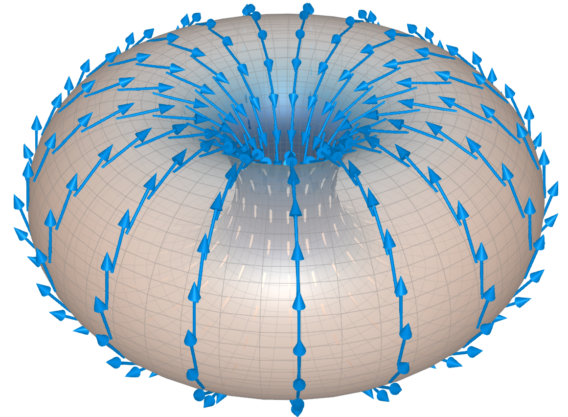
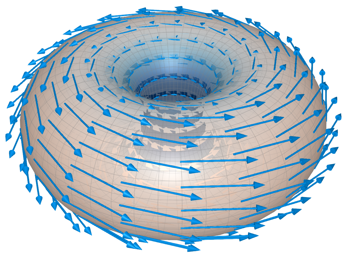
Figure 3. Illustration of the vector fields $\phi_{1}$ (left) and $\phi_{2}$ (right).

We apply Algorithm 1 in the following settings:

1. A somewhat weak vector field with $\theta=(-2,2)$, where we condition the process on a point obtained from forward simulation of the unconditional process (Figure 4, guided processes obtained with $\lambda=0.95$). One can visually assess that samples of the guided process the original forward path.

2. A stronger vector field with $\theta=(-1,8)$, where we condition the process on a point obtained from forward simulation of the unconditional process (Figure 5, guided processes obtained with $\lambda=0.99$). Due to the strong drift, paths should take a turn around the torus. Indeed, samples of the guided process do so.

3. A very weak vector field with $\theta=(-1,0.1)$, where we condition the process on a point which is unlikely under the forward unconditional process (Figure 6, guided processes obtained with $\lambda=0.7$). In this case, samples from the guided process can either go clockwise or counterclockwise, the latter seemingly more likely. In this case, in Table 1 we also report how the choice of $\lambda$ affects the acceptance rate in Algorithm 1.

In all cases the right-hand-plot displays every 50-th sample obtained from 1000 iterations of Algorithm 1.

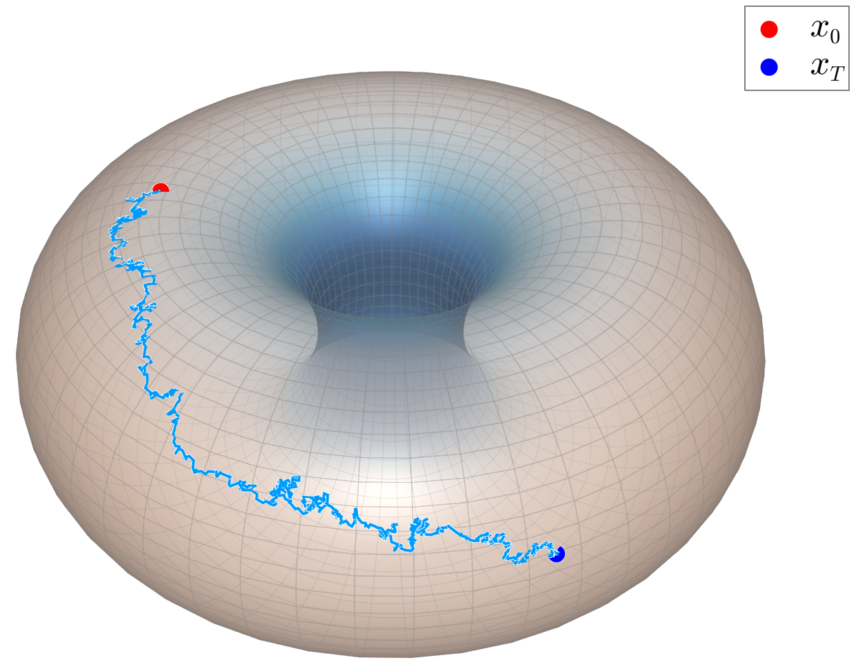
Figure 4. Left: Forward simulation of unconditional process $X$. Right: final 6 accepted samplepaths of 1000 repetitions of Algorithm 1 of bridge processes starting at $(3,0,2)$ conditioned to hit $X_{T}$ at time $T=1$. We used the vector field described in (5.2) with $\theta=(-2,2)$. The acceptance rate was 17%.

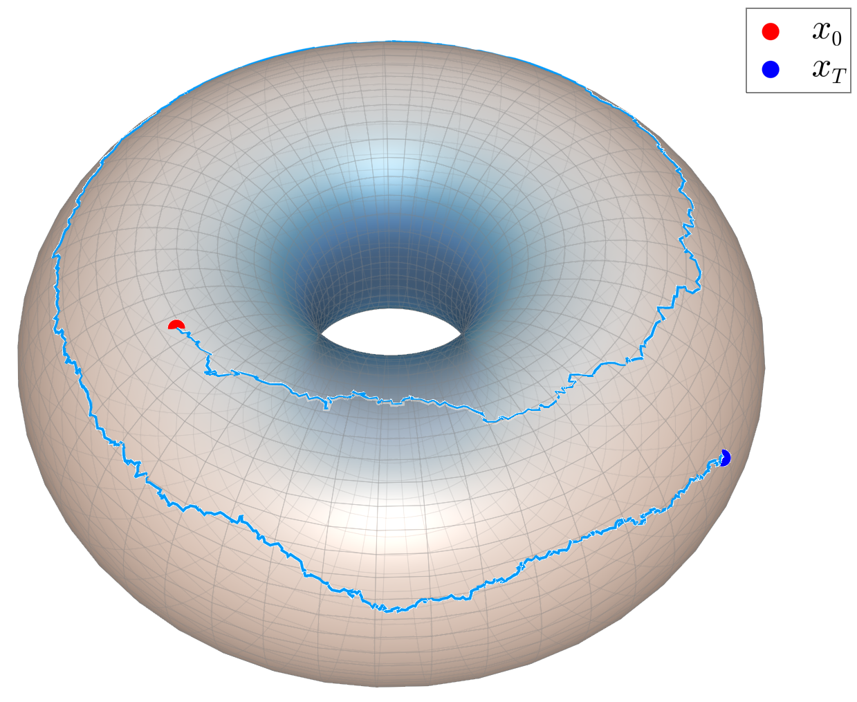
Figure 5. Left: Forward simulation of $X$. Right: final 6 accepted samplepaths of 1000 repetitions of Algorithm 1 of bridge processes starting at $(3,0,2)$ conditioned to hit $X_{T}$ at time $T=1$. We used the vector field described in (5.2) with $\theta=(-1,8)$. The acceptance rate was 19.5%.

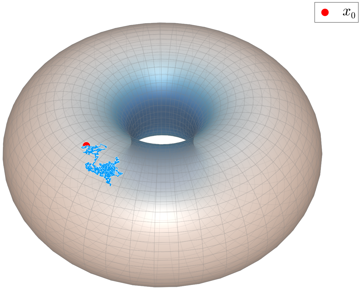
Figure 6. Left: Forward trajectory of the unconditioned process Right: One trajectory for each 20 accepted proposals of Algorithm 1 for the process conditioned on hitting $(-3,0,2)$. A darker color indicates a later iteration of the algorithm. The vector field (5.2) with $\theta=(-1,0.1)$ was applied.

$\lambda$	0.0	0.5	0.7	0.9	0.99
acceptance rate	10%	27%	39%	60%	89%

Table 1. Acceptance rate for various choices of $\lambda$ for the 3rd setting considered (Figure 6).

5.2. Parameter estimation

Here, we perform inference on the parameter $\theta$ in (5.2) based on observations $\mathcal{D}=\{X_{t_{i}}=x_{i},\,i=1,\dots,n\}$. To perform parameter inference conditional on $\mathcal{D}$, we simultaneously sample $\theta,X\mid\mathcal{D}$. This can be done using Gibbs-type sampling method in which we repeatedly perform the following steps

1. Update $Z\mid(\mathcal{D},\theta)$ using steps 2–4 of Algorithm 1 and set $U=\mathcal{GP}_{\theta}(x_{0},Z)$.

2. Update $\theta\mid(\mathcal{D},X)$, where $X=\pi(U)$.

3. Compute $Z$ as the anti-development of $X$ under the drift with parameter $\theta$.

Step (2) requires an update of $\theta$. To do this, we utilize the following conjugacy result, based on Proposition 4.5 of Mider et al., (2021) for normal priors. It follows from Girsanov’s theorem, see e.g. Proposition 1B of Elworthy, (1988) , that if we assign a prior $\pi(\theta)$ to $\theta$ then

$$\pi(\theta\mid Z,X)\propto\exp\left(\int_{0}^{t_{n}}\left\langle V_{\theta}(X_{s}),\,\mathrm{d}X_{s}\right\rangle_{X_{s}}-\frac{1}{2}\int_{0}^{t_{n}}\left\langle V_{\theta}(X_{s}),V_{\theta}(X_{s})\right\rangle_{X_{s}}\,\mathrm{d}s\right)\pi(\theta).$$

Hence, if $\theta\sim N(0,\Gamma_{0}^{-1})$, then $\theta\mid X,Z\sim N(\Gamma^{-1}\mu,\Gamma^{-1})$, where,

$$\mu =\begin{pmatrix}\int_{0}^{t_{n}}\left\langle\phi_{k}(X_{s}),\,\mathrm{d}X_{s}\right\rangle_{X_{s}}\end{pmatrix}_{k=1}^{K}$$

$$\Gamma =\begin{pmatrix}\int_{0}^{t_{n}}\left\langle\phi_{k}(X_{s}),\phi_{\ell}(X_{s})\right\rangle_{X_{s}}\,\mathrm{d}s\end{pmatrix}_{k,\ell=1}^{K}+\Gamma_{0}$$

We applied this Gibbs sampler to a dataset generated under forward simulating $X$ with vector field (5.2) with $\theta=(4,-4)$ and saving its values at $40$ equidistant times. The posterior samples are displayed in Figure 7. For the prior, we used $\Gamma_{0}=0.05I$ and we used tuning parameter $\lambda=0.9$ in the Crank-Nicolson steps.

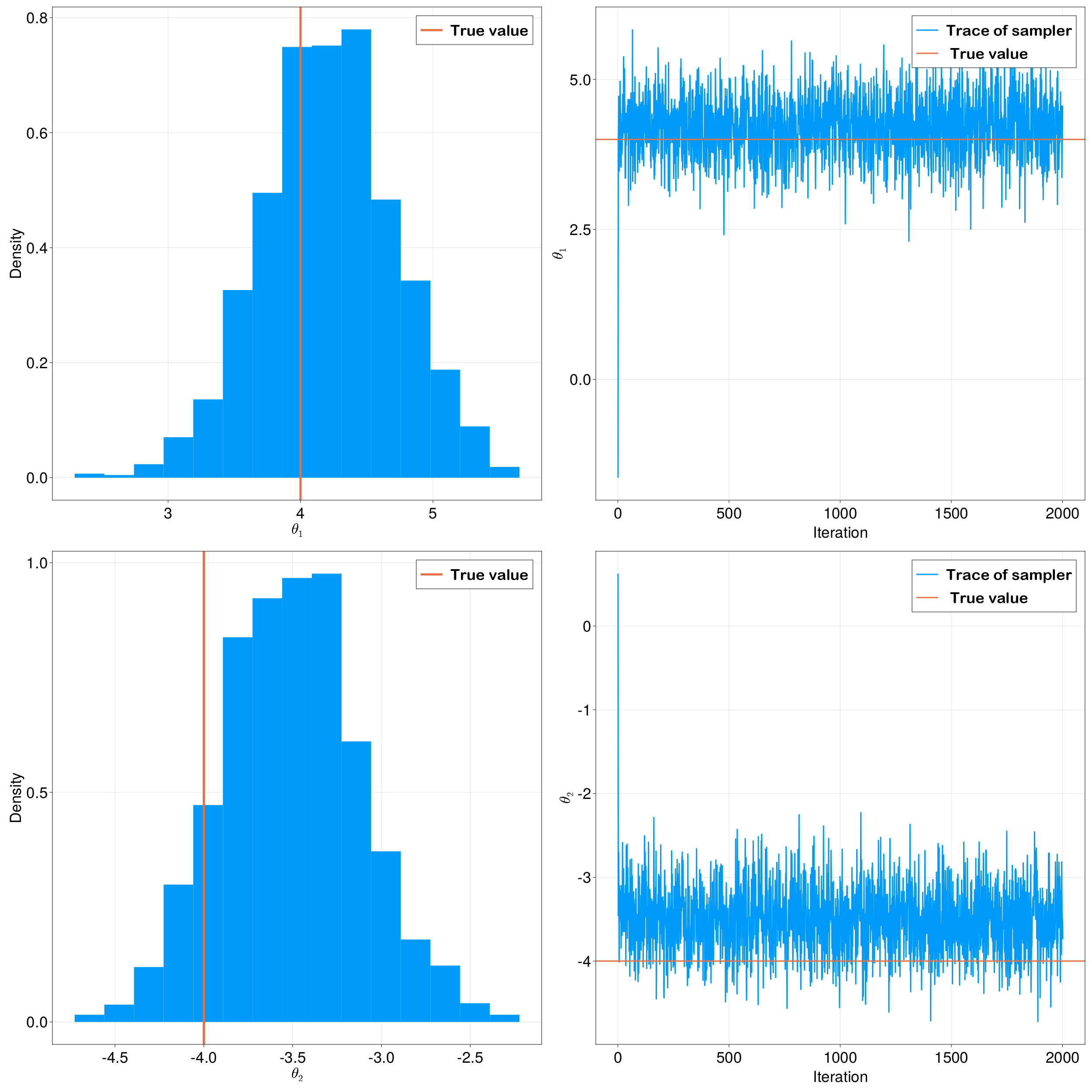
Figure 7. Left: Histograms 1900 samples from the posterior distribution of $\theta$ after 100 iteration of burn-in time using the Gibbs sampler Right: Trace of the sampler. The top row are the samples for $\theta_{1}$, the bottom row the samples for $\theta_{2}$. Data were generated with $(\theta_{1},\theta_{2})=(4,-4)$ as indicated by the red lines.

6. Other types of conditionings

Up to this point, we have considered the problem of diffusion bridge simulation, where $h(t,x)=p(t,x;T,x_{T})$. We now consider variants of this problem.

First consider the following model

$$(X_{t},\,t\in[0,T]) \sim{\mathbb{P}}$$

$$V\mid X_{T}=x_{T} \sim q_{V\mid X_{T}}(\cdot\mid x_{T})$$

for a conditional density $q_{V\mid X_{T}}$. This model corresponds to observing a realisation $v$ from the conditional distribution given $V\mid X_{T}=x_{T}$. Suppose interest lies in the distribution of $X_{T}\mid V=v$. If we let the measure ${\mathbb{P}}^{h}$ be the measure induced by

$$h(t,x)=\int p(t,x;T,z)q_{V\mid X_{T}}(v\mid z)\,\mathrm{d}\mathrm{Vol}_{M}(z).$$ (6.1)

then $\mathfrak{A}h=0$ and $h\in\mathcal{H}$.

As in Example 2.4 in Corstanje et al., (2023), for test functions $f\colon M\to\mathbb{R}$

$${\mathbb{E}}^{h}f(X_{t})=\int_{M}{\mathbb{E}}\left(f(X_{t})\mid X_{T}=z\right)q_{X_{T}\mid V}(z\mid v)\,\mathrm{d}\mathrm{Vol}_{M}(z),$$

where

$$q_{X_{T}\mid V}(z\mid v)=\frac{p(0,x_{0};T,z)q_{V\mid X_{T}}(v\mid z)}{h(0,x_{0})}$$

is the conditional density of $X_{T}\mid V=v$ with respect to the volume measure. Hence, sampling under ${\mathbb{P}}^{h}$ is equivalent to first sampling $x_{T}$ from the distribution of $X_{T}\mid V=v$ and subsequently sampling a bridge connecting $x_{0}$ at time $0$ and $z$ at time $T$.

In a variant, one can take any density function $q(z)$ with respect to the volume measure to obtain a transformation as follows:

$$h(t,x)=\int\frac{p(t,x;T,z)q(z)}{p(0,x_{0};T,z)}\,\mathrm{d}\mathrm{Vol}_{M}(z).$$ (6.2)

This corresponds to a conditioning where $X$ started in $X_{0}=x_{0}$ and forced into the marginal distribution with density $q$ at time $T$, such as seen in in Baudoin, (2002). This is important for generative diffusion models on manifolds.

7. Proofs

The proofs in Sections 7.2 and 7.3 are derived from the following theorem, which is a slight reformulation of Theorem 3.3 of Corstanje et al., (2023).

Theorem 7.1.

Let $g,h\in\mathcal{H}$. Suppose there exists a $t_{0}\in[0,T)$ and a family of $\mathcal{F}_{t}$-measurable events $\{A_{k}^{t}\}_{k}$ for all $t\in[t_{0},T)$ such that

1. For all $k$ and $t_{0}\leq s\leq t<T$, $A_{k}^{t}\subseteq A_{k+1}^{t}$ and $A_{k}^{t}\subseteq A_{k}^{s}$. We denote the limits by

   $$A^{t}=\bigcup_{k}A_{k}^{t},\qquad A_{k}^{T}=\bigcap_{t<T}A_{k}^{t},\qquad A^{T}=\bigcap_{t<T}A^{t}$$

2. ${\mathbb{E}}\left(g(t,X_{t})\mid\mathcal{F}_{s}\right)$ is ${\mathbb{P}}$-almost surely bounded uniformly in $t$ and for all $s\in[t_{0},T)$ and $x\in M$,

   $$\lim_{t\uparrow T}{\mathbb{E}}\left(g(t,X_{t})\mid X_{s}=x\right)=h(s,x)$$

3. $$\lim_{k\to\infty}\lim_{t\uparrow T}{\mathbb{E}}^{h}\left(\frac{g(t,X_{t})}{h(t,X_{t})}\mathbf{1}_{A_{k}^{t}}\right)=1$$

4. For all $k$,

   $$\exp\left(\int_{0}^{t}\frac{{\mathfrak{A}}g(s,X_{s})}{g(s,X_{s})}\,\mathrm{d}s\right)\mathbf{1}_{A_{k}^{t}}$$

   is ${\mathbb{P}}^{g}$-almost surely uniformly bounded in $t$ on $[t_{0},T)$.

5. ${\mathbb{P}}^{g}(A^{T})=1$.

Then ${\mathbb{P}}_{T}^{h}\sim{\mathbb{P}}_{T}^{g}$ with

$$\frac{\,\mathrm{d}{\mathbb{P}}^{h}_{T}}{\,\mathrm{d}{\mathbb{P}}^{g}_{T}}=\frac{g(0,X_{0})}{h(0,X_{0})}\exp\left(\int_{0}^{T}\frac{{\mathfrak{A}}g(s,X_{s})}{g(s,X_{s})}\,\mathrm{d}s\right)$$ (7.1)

7.1. Proof of Theorem 4.1

Suppose $X$ has infinitesimal generator $\left({\mathfrak{L}}_{X},{\mathfrak{D}}\left({\mathfrak{L}}_{X}\right)\right)$. Let $f\colon N\to{\mathbb{R}}$ be such that $f\circ\Phi\in{\mathfrak{D}}\left(\mathfrak{L}_{X}\right)$. Then the infinitesimal generator ${\mathfrak{L}}_{Y}$ of $Y$ satisfies

$${\mathfrak{L}}_{Y}f(y) =\lim_{t\downarrow 0}\frac{{\mathbb{E}}\left(f(Y_{t})\mid Y_{0}=y\right)-f(y)}{t}$$ (7.2)

$$=\lim_{t\downarrow 0}\frac{{\mathbb{E}}\left((f\circ\Phi)(X_{t})\mid X_{0}=\Phi^{-1}(y)\right)-(f\circ\Phi)\left(\Phi^{-1}(y)\right)}{t}$$

$$={\mathfrak{L}}_{X}\left(f\circ\Phi\right)\left(\Phi^{-1}(y)\right),$$

For $f\colon[0,T]\times N\to{\mathbb{R}}$, let the pullback $\Phi^{*}f\colon[0,T]\times M\to{\mathbb{R}}$ given by $(\Phi^{*}f)(t,x)=f(t,\Phi(x))$ be in the domain of ${\mathfrak{A}}_{X}$. Then we have

$$\mathfrak{A}_{Y}f(t,y)=\left({\mathfrak{A}}_{X}(\Phi^{*}f)\right)\left(t,\Phi^{-1}(y)\right),\quad t\in[0,T],\quad y\in N.$$

Take $f=\Phi_{*}h$, then $\Phi^{*}f(t,x)=(\Phi_{*}h)(t,\Phi(x))=h(t,x)$ is in the domain of ${\mathfrak{A}}_{X}$, by assumption. The preceding display therefore gives

$$({\mathfrak{A}}_{Y}\Phi_{*}h)(t,y)=({\mathfrak{A}}_{X}h)(t,\Phi^{-1}(y))=\left(\Phi_{*}({\mathfrak{A}}_{X}h)\right)(y),$$ (7.3)

where the second equality follows from the definition of $\Phi_{*}h$.

We have (cf. Equation 3.1)

$$E_{t}^{\Phi_{*}h}(Y)=\frac{\Phi_{*}h(t,Y_{t})}{\Phi_{*}h(0,Y_{0})}\exp\left(-\int_{0}^{t}\frac{{\mathfrak{A}}_{Y}(\Phi_{*}h)(s,Y_{s})}{\Phi_{*}h(s,Y_{s})}\,\mathrm{d}s\right)$$

By Equation 7.3, ${\mathfrak{A}}_{Y}(\Phi_{*}h)(s,Y_{s})=({\mathfrak{A}}_{X}h)(s,\Phi^{-1}(Y_{s}))=({\mathfrak{A}}_{X}h)(s,X_{s})$. By definition of $\Phi_{*}h$ we have $\Phi_{*}h(t,Y_{t})=h(t,X_{t})$. Substituting these two results in the previous display we obtain $E_{t}^{\Phi_{*}h}(Y)=E_{t}^{h}(X)$. This implies

$$\mathbb{E}\psi\left(\Phi(X^{h})\right)=\mathbb{E}\left[\psi(\Phi(X))E_{t}^{h}(X)\right]=\mathbb{E}\left[\psi(Y)E_{t}^{\Phi_{*}h}(Y)\right].$$

7.2. Proof of 4.2

We start with a lemma used in the proof.

Lemma 7.2.

$Y$ admits a transition density $p_{Y}(s,y;t,z)=p(s,\Phi^{-1}(y);t,\Phi^{-1}(z))$ with respect to the measure on $N$ obtained from the pushforward Riemannian volume measure on $M$ through $\Phi$, $\Phi_{*}\left(\mathrm{Vol}_{M}\right)$.

Proof.

For $A\subseteq N$ measurable, $y\in N$ and $s\leq t$, we have

$${\mathbb{P}}(Y_{t}\in A\mid Y_{s}=y) ={\mathbb{P}}\left(X_{t}\in\Phi^{-1}(A)\mid X_{s}=\Phi^{-1}(y)\right)$$

$$=\int_{\Phi^{-1}(A)}p\left(s,\Phi^{-1}(y);t,u\right)\,\mathrm{d}\mathrm{Vol}_{M}(u)$$

$$=\int_{A}p(s,\Phi^{-1}(y);t,\Phi^{-1}(z))\,\mathrm{d}\Phi_{*}\left(\mathrm{Vol}_{M}\right)(z),$$

where the last equality follows from the substitution rule, see e.g. Proposition 4.4.12 of Lovett, (2010) ∎

Proof of 4.2.

As (7.1a) is satasfied by default, we check assumptions (7.1b), (7.1c) (7.1d) and (7.1e) for $Y$, $\Phi_{*}g$, $\Phi_{*}h$ and events $\{A^{t}_{k}\}_{k}$.

Assumption (7.1b) is satisfied since

$${\mathbb{E}}\left(\Phi_{*}g(t,Y_{t})\mid Y_{s}=y\right) =\int g(t,\Phi^{-1}(z))p_{Y}(s,y;T,z)\,\mathrm{d}\Phi_{*}\left(\mathrm{Vol}_{M}\right)(z)$$

$$=\int g(t,\Phi^{-1}(z))p(s,\Phi^{-1}(y);T,\Phi^{-1}(z))\,\mathrm{d}\Phi_{*}\left(\mathrm{Vol}_{M}\right)(z)$$

$$=\int g(t,x)p(s,\Phi^{-1}(y);T,x)\,\mathrm{d}\mathrm{Vol}_{M}(x)$$

$$\to h(s,\Phi^{-1}(y))=\Phi_{*}h(s,y),\quad\text{as}\>t\uparrow T$$

Assumption (7.1c) is satisfied since

$$\lim_{k\to\infty}\lim_{t\uparrow T}{\mathbb{E}}^{\Phi_{*}h}\left(\frac{\Phi_{*}g(t,Y_{t})}{\Phi_{*}{h}(t,Y_{t})}\mathbf{1}_{A_{k}^{t}}\right)=\lim_{k\to\infty}\lim_{t\uparrow T}{\mathbb{E}}^{h}\left(\frac{g(t,X_{t})}{h(t,X_{t})}\mathbf{1}_{A_{k}^{t}}\right)=1.$$

Here, the first equality follows from $E_{t}^{\Phi_{*}h}(Y)=E_{t}^{h}(X)$, which was derived in the proof of 4.1. The final equality follows since ${\mathbb{Q}}^{\Phi_{*}h}$ is the pushforward measure ${\mathbb{P}}^{h}$ under $\Phi$.

To see that Assumption (7.1d) is satisfied, note that from the proof of 4.1, we obtain ${\mathfrak{A}}_{Y}(\Phi_{*}g)(s,Y_{s})=({\mathfrak{A}}_{X}g)(s,X_{s})$ and thus

$$\exp\left(\int_{0}^{t}\frac{\mathfrak{A}_{Y}\Phi_{*}g(s,Y_{s})}{\Phi_{*}g(s,Y_{s})}\,\mathrm{d}s\right)=\exp\left(\int_{0}^{t}\frac{\mathfrak{A}_{X}g(s,X_{s})}{g(s,X_{s})}\,\mathrm{d}s\right),$$

which verifies the assumption.

For (7.1e), we note that $E_{t}^{g}(X)=E_{t}^{\Phi_{*}g}(\Phi(X))$ and thus the measures ${\mathbb{Q}}^{\Phi_{*}g}$ and ${\mathbb{P}}^{g}$ define the same probability $1$ sets. ∎

7.3. Proof of 3.4

We also need the following two results where we assume $M$ to be a compact manifold.

Theorem 7.3 (Theorem 5.3.4 of Hsu, (2002)).

For all $t\in(0,T)$ and $x,y\in M$,

$$\frac{C_{1}}{t^{d/2}}\exp\left(-\frac{{\mathrm{dist}}(x,y)^{2}}{2t}\right)\leq\kappa(t,x,y)\leq\frac{C_{2}}{t^{(2d-1)/2}}\exp\left(-\frac{{\mathrm{dist}}(x,y)^{2}}{2t}\right)$$

Theorem 7.4 (Theorem 5.5.3 of Hsu, (2002)).

There is a constant $C$ such that for all $t\in(0,T)$ and $x,y\in M$,

$$\left\lvert\nabla\log\kappa(t,x,y)\right\rvert\leq C\left(\frac{{\mathrm{dist}}(x,x_{T})}{t}+\frac{1}{\sqrt{t}}\right)$$

Proof of 3.4.

Let $\eta(t)=(T-t)^{\varepsilon}$ for $\varepsilon\in(0,1/2)$ and define the function

$$\zeta(t,x)=-\eta(t)\log g(t,x),$$ (7.4)

We recall that $g(t,x)=\kappa(T-t,x,x_{T})$. It follows from 7.3 that

$$\beta_{1}(t)+\eta(t)\frac{{\mathrm{dist}}(x,x_{T})^{2}}{2(T-t)}\leq\zeta(t,x)\leq\beta_{2}(t)+\eta(t)\frac{{\mathrm{dist}}(x,x_{T})^{2}}{2(T-t)}$$ (7.5)

where

$$\beta_{1}(t) =-\eta(t)\log\left(\frac{C_{2}}{(T-t)^{(2d-1)/2}}\right)$$ (7.6)

$$\beta_{2}(t) =-\eta(t)\log\left(\frac{C_{1}}{(T-t)^{d/2}}\right)$$

Now let $t_{0}\in[0,T)$ be such that $\beta_{2}(t)\geq\beta_{1}(t)\geq 0$ for all $t\in[t_{0},T)$ and observe that $\eta$ and $t_{0}$ are such that

1. $\eta(t)\geq 0$ and $\zeta(t,x)\geq 0$ for all $t\in[t_{0},T)$

2. $t\mapsto\frac{\eta(t)}{T-t}$ is integrable on $[t_{0},T)$

3. $t\mapsto\eta(t)\log\left(\frac{1}{T-t}\right)$ is bounded on $[t_{0},T)$

Define the collection of events $A_{k}^{t}$ as

$$A_{k}^{t}=\left\{\sup_{t_{0}\leq s<t}\zeta(s,X_{s})\leq k\right\},\qquad t\in[t_{0},T),k=1,2,\dots.$$ (7.7)

Then (7.1a) is satisfied by construction. By Theorem 4.1.4 (3) of Hsu, (2002),

$$\lim_{t\uparrow T}{\mathbb{E}}\left(g(t,X_{t})\mid X_{s}=x\right) =\lim_{t\uparrow T}\int\kappa({T-t},y,x_{T})p(s,x;t,y)\,\mathrm{d}\mathrm{Vol}_{M}(y)$$ (7.8)

$$=p(s,x;T,x_{T})=h(s,x)$$

and thus (7.1b) is satisfied as well. For (7.1c), we first note that

$${\mathbb{E}}^{h}\left(\frac{g(t,X_{t})}{h(t,X_{t})}\mathbf{1}_{A_{k}^{t}}\right)={\mathbb{E}}^{h}\left(\frac{g(t,X_{t})}{h(t,X_{t})}\right)-{\mathbb{E}}^{h}\left(\frac{g(t,X_{t})}{h(t,X_{t})}\mathbf{1}_{(A_{k}^{t})^{c}}\right)$$

By 7.5, the first term tends to 1 as $t\uparrow T$. Therefore it suffices to show that the second term tends to $0$ upon taking $\lim_{k\to\infty}\lim_{t\uparrow T}$ to prove that (7.1c) is satisfied. To show this, we consider the sequence of stopping times $\sigma_{k}=T\wedge\inf\{t\geq 0:\zeta(t,X_{t})>k\}$ and observe that $(A_{k}^{t})^{c}=\{t>\sigma_{k}\}$. Now

$${\mathbb{E}}^{h}\left(\frac{g(t,X_{t})}{h(t,X_{t})}\mathbf{1}_{\{t>\sigma_{k}\}}\right) ={\mathbb{E}}\left(\frac{g(t,X_{t})}{h(0,x_{0})}\mathbf{1}_{\{t>\sigma_{k}\}}\right)$$

$$={\mathbb{E}}\left(\frac{\mathbf{1}_{\{t>\sigma_{k}\}}}{h(0,x_{0})}{\mathbb{E}}\left(g(t,X_{t})\mid\mathcal{F}_{\sigma_{k}}\right)\right)$$

$$={\mathbb{E}}\left(\frac{\mathbf{1}_{\{t>\sigma_{k}\}}}{h(0,x_{0})}\int_{M}p(\sigma_{k},X_{\sigma_{k}};t,z)g(t,z)\,\mathrm{d}z\right)$$

Here, the first equality follows from applying the change of measure (3.2) with ${\mathfrak{A}}h=0$. By3.3, we obtain an upper bound given by

$${\mathbb{E}}\left(\frac{\mathbf{1}_{\{t>\sigma_{k}\}}}{h(0,x_{0})}\gamma_{1}e^{-\gamma_{3}(t-\sigma_{k})}\int_{M}\kappa(\gamma_{2}(t-\sigma_{k}),X_{\sigma_{k}},z)\kappa(T-t,z,x_{T})\,\mathrm{d}\mathrm{Vol}_{M}(z)\right)$$

It follows from the Chapman-Kolmogorov relations, see e.g. Theorem 4.1.4 (5) of Hsu, (2002), that this is equal to

$${\mathbb{E}}\left(\frac{\mathbf{1}_{\{t>\sigma_{k}\}}}{h(0,x_{0})}\gamma_{1}e^{-\gamma_{3}(t-\sigma_{k})}\kappa\left(\gamma_{2}(t-\sigma_{k})+T-t,X_{\sigma_{k}},x_{T})\right)\right).$$

By 7.3, we can find a positive constant $\gamma_{4}$ such that this expression is bounded by

$$\begin{gathered}{\mathbb{E}}\left(\frac{\mathbf{1}_{\{t>\sigma_{k}\}}}{h(0,x_{0})}\gamma_{1}e^{-\gamma_{3}(t-\sigma_{k})}\gamma_{4}\left(\gamma_{2}(t-\sigma_{k})+T-t\right)^{-(2d-1)/2}\right.\\ \left.\times\exp\left(-\frac{{\mathrm{dist}}(X_{\sigma_{k}},x_{T})^{2}}{2\gamma_{2}(t-\sigma_{k})+2(T-t)}\right)\right)\end{gathered}$$

Now observe that

1. Since $X$ is continuous in time, $\zeta\left(\sigma_{k},X_{\sigma_{k}}\right)=k$. It thus follows from (7.5) that

   $$\frac{k-\beta_{2}(\sigma_{k})}{\eta(\sigma_{k})}\leq\frac{{\mathrm{dist}}(X_{\sigma_{k}},x_{T})^{2}}{2(T-\sigma_{k})}\leq\frac{k-\beta_{1}(\sigma_{k})}{\eta(\sigma_{k})}$$

2. $e^{-\gamma_{3}(t-\sigma_{k})}\leq 1$ on $\{t>\sigma_{k}\}$

3. Let $\underline{\gamma}=\gamma_{2}\wedge 1$ and $\bar{\gamma}=\gamma_{2}\vee 1$. Then $\underline{\gamma}(T-\sigma_{k})\leq\gamma_{2}(t-\sigma_{k})+T-t\leq\bar{\gamma}(T-\sigma_{k})$.

It now follows from the preceding, combined with observations 1–3 that a positive constant $\gamma_{5}$ exists such that

$${\mathbb{E}}^{h}\left(\frac{g(t,X_{t})}{h(t,X_{t})}\mathbf{1}_{\{t>\sigma_{k}\}}\right) \leq{\mathbb{E}}\left(\gamma_{5}\mathbf{1}_{\{t>\sigma_{k}\}}(T-\sigma_{k})^{-(2d-1)/2}\exp\left(-\frac{k-\beta_{2}(\sigma_{k})}{\eta(\sigma_{k})\bar{\gamma}}\right)\right)$$

$$={\mathbb{E}}\left(\gamma_{5}C_{1}^{-1/\bar{\gamma}}\mathbf{1}_{\{t>\sigma_{k}\}}(T-\sigma_{k})^{-\frac{2d-1}{2}-\frac{d}{2\bar{\gamma}}}\exp\left(-\frac{k}{\eta(\sigma_{k})\bar{\gamma}}\right)\right)$$

We now substitute $\eta(t)=(T-t)^{\varepsilon}$. Upon noting that trivially $\tau:=T-\sigma_{k}\in[0,T]$, we deduce that

$${\mathbb{E}}^{h}\left(\frac{g(t,X_{t})}{h(t,X_{t})}\mathbf{1}_{\{t>\sigma_{k}\}}\right)\leq\gamma_{5}C_{1}^{-1/\bar{\gamma}}\sup_{0\leq\tau<\infty}\tau^{-\gamma_{6}}\exp\left(-\frac{k}{\bar{\gamma}}\tau^{-\varepsilon}\right),$$

where $\gamma_{6}=(2d-1)/2+d/(2\bar{\gamma})$. The function of $\tau$ over which the $\sup$ is taken is concave and attains it’s maximum at $\left(\gamma_{6}\bar{\gamma}/(k\varepsilon)\right)^{-1/\varepsilon}$. Hence,

$${\mathbb{E}}^{h}\left(\frac{g(t,X_{t})}{h(t,X_{t})}\mathbf{1}_{\{t>\sigma_{k}\}}\right)\leq\gamma_{5}C_{1}^{-1/\bar{\gamma}}\left(\frac{\varepsilon}{\gamma_{6}\bar{\gamma}}\right)^{-\gamma_{6}/\varepsilon}k^{-\gamma_{6}/\varepsilon}\exp\left(-\frac{\gamma_{6}}{\varepsilon}\right)$$ (7.9)

Since, (7.9) tends to $0$ as $k\to\infty$, (7.1c) is satisfied.

For (7.1d), note that as $\partial_{t}g+\frac{1}{2}\Delta g=0$, ${\mathfrak{A}}g=\left({\mathfrak{L}}-\frac{1}{2}\Delta\right)g$. Hence, ${\mathfrak{A}}g/g=V(\log g)$. Clearly, by the Cauchy-Schwarz inequality

$$\left\lvert V(\log g)(t,x)\right\rvert\leq\left\lvert V(x)\right\rvert\left\lvert\nabla\log g\right\rvert$$

Since $V$ is smooth and $M$ is compact, $\left\lvert V\right\rvert$ is bounded. Hence, by 7.4, there exists a constant $C$ such that

$$\left\lvert V(\log g)(t,x)\right\rvert\leq C\left(\frac{{\mathrm{dist}}(x,x_{T})}{T-t}+\frac{1}{\sqrt{T-t}}\right)$$

Now notice that, by (7.5), on $A_{k}^{t}$, we have that

$${\mathrm{dist}}(X_{t},x_{T})\leq\sqrt{2(T-t)^{1-\varepsilon}\left(k-\beta_{1}(t)\right)}$$ (7.10)

Hence, we obtain that

$$\left\lvert V(\log g)(t,X_{t})\right\rvert\mathbf{1}_{A_{k}^{t}}\leq C\left(\frac{\sqrt{2(k-\beta_{1}(t))}}{\sqrt{(T-t)^{1+\varepsilon}}}+\frac{1}{\sqrt{T-t}}\right)$$

Since the above term is integrable on $[0,T]$, (7.1d) is satisfied. We proof (7.1e) separately in 7.6. The result now follows from 7.1, where the form of the Radon-Nikodym derivative in Equation 7.1 follows from the observation that ${\mathfrak{A}}g/g=V(\log g)$.

∎

Lemma 7.5.

Suppose (7.1b) is satisfied and let $s<T$. For any bounded $\mathcal{F}_{s}$-measurable function $f_{s}$,

$$\lim_{t\uparrow T}{\mathbb{E}}^{h}\left(f_{s}(X)\frac{g(t,X_{t})}{h(t,X_{t})}\right)={\mathbb{E}}^{h}f_{s}(X)$$

Proof.

Since, $\,\mathrm{d}{\mathbb{P}}_{t}^{h}=h(t,X_{t})/h(0,x_{0})\,\mathrm{d}{\mathbb{P}}_{t}$,

$$\lim_{t\uparrow T}{\mathbb{E}}^{h}\left(f_{s}(X)\frac{g(t,X_{t})}{h(t,X_{t})}\right) =\lim_{t\uparrow T}{\mathbb{E}}\left(\frac{f_{s}(X)}{h(0,x_{0})}g(t,X_{t})\right)$$ (7.11)

$$=\lim_{t\uparrow T}{\mathbb{E}}\left(\frac{f_{s}(X)}{h(0,x_{0})}{\mathbb{E}}\left(g(t,X_{t})\mid\mathcal{F}_{s}\right)\right)$$

$$=={\mathbb{E}}\left(f_{s}(X)\frac{h(s,X_{s})}{h(0,x_{0})}\right)={\mathbb{E}}^{h}f_{s}(X)$$

Here, the second but last equality follows from (7.1b) and dominated convergence. ∎

Theorem 7.6.

Let $A_{k}^{t}$ be defined as in (7.7). Then ${\mathbb{P}}^{g}(A^{T})=1$.

Proof.

To reduce notation, we write a subscript $t$ to indicate evaluation in $(t,X_{t})$ for functions of $(t,x)\in[t_{0},T)\times M$. It is sufficient to show that $\zeta_{t}$ is ${\mathbb{P}}^{g}$-almost surely bounded as $t\uparrow T$. To do this, we find an upper bound on

$$\xi_{t}:=\zeta_{t}-\beta_{1}(t),$$ (7.12)

which in turn yields the result as $\beta_{1}(t)\downarrow 0$ as $t\uparrow T$.

Notice that, under ${\mathbb{P}}^{g}$, by Itô’s formula,

$$\xi_{t}=\xi_{t_{0}}+M_{t}^{\xi}+\int_{t_{0}}^{t}{\mathfrak{A}}^{g}\xi_{s}\,\mathrm{d}s,$$ (7.13)

where $M^{\xi}$ denotes the process

$$M^{\xi}_{t}=\int_{t_{0}}^{t}\eta(s)\nabla\log g_{s}\,\mathrm{d}W_{s}$$

The remainder of the proof is structured as follows: First we find an upper bound of $M_{t}^{\xi}+\int_{t_{0}}^{t}{\mathfrak{A}}^{g}\xi_{s}\,\mathrm{d}s$ in terms of functions of $t$ and $\xi$. Then we apply a generalized Grönwall inequality to find an upper bound for $\xi_{t}$, which is bounded as $t\uparrow T$.

First observe that

$$M_{t}^{\xi}=M_{t}^{\xi}-\frac{1}{2}\left[M^{\xi}\right]_{t}+\frac{1}{2}\int_{t_{0}}^{t}\left\lvert\eta(s)\nabla\log g_{s}\right\rvert^{2}\,\mathrm{d}s$$ (7.14)

By Lemma A.2 of Corstanje et al., (2023), there exists an almost surely finite random variable $C$ such that

$$M_{t}^{\xi}-\frac{1}{2}\left[M^{\xi}\right]_{t}\leq C\log\left(\frac{1}{T-t}\right).$$ (7.15)

Moreover, we infer from (7.5) that

$${\mathrm{dist}}(X_{t},x_{T})\leq\sqrt{\frac{2(T-t)\xi_{t}}{\eta(t)}}$$

Hence, by 7.4, there is a positive constant $c_{1}$ such that

$$\left\lvert\nabla\log g_{t}\right\rvert\leq c_{1}\left(\sqrt{\frac{2\xi_{t}}{\eta(t)(T-t)}}+\frac{1}{\sqrt{T-t}}\right)$$ (7.16)

Therefore, by combining (7.14) with (7.15) and (7.16), we find a bound on $M^{\xi}_{t}$ in terms of $t$ and $\xi$ through

$$M_{t}^{\xi}\leq C\log\left(\frac{1}{T-t}\right)+\frac{c_{1}^{2}}{2}\int_{t_{0}}^{t}\eta(s)^{2}\left(\sqrt{\frac{2\xi_{s}}{\eta(s)(T-s)}}+\frac{1}{\sqrt{T-s}}\right)\,\mathrm{d}s$$ (7.17)

Next, we study ${\mathfrak{A}}^{g}\xi$. A direct computation yields that

$${\mathfrak{A}}^{g}\xi_{t} ={\mathfrak{A}}^{g}\zeta_{t}-\partial_{t}\beta_{1}$$ (7.18)

$$={\mathfrak{A}}^{g}\zeta_{t}+\log\left(\frac{C_{2}}{(T-t)^{(2d-1)/2}}\right)\partial_{t}\eta(t)+\eta(t)\partial_{t}\log\left(\frac{C_{2}}{(T-t)^{(2d-1)/2}}\right)$$

$$={\mathfrak{A}}^{g}\zeta_{t}+\eta(t)\log\left(\frac{C_{2}}{(T-t)^{(2d-1)/2}}\right)\partial_{t}\log\eta(t)+\eta(t)\frac{2d-1}{2(T-t)}$$

$$={\mathfrak{A}}^{g}\zeta_{t}-\beta_{1}(t)\partial_{t}\log\eta(t)+\eta(t)\frac{2d-1}{2(T-t)}$$

In order to compute ${\mathfrak{A}}^{g}$, we apply the identity

$$\partial_{t}\log g+\frac{1}{2}\Delta\log g=-\frac{1}{2}\left\lvert\log g\right\rvert^{2}$$

This yields

$${\mathfrak{A}}^{g}\zeta_{t} =-\log g_{t}\partial_{t}\eta(t)-\eta(t)\partial_{t}\log g_{t}-\eta(t){\mathfrak{L}}^{g}(\log g)_{t}$$ (7.19)

$$=\zeta_{t}\partial_{t}\log\eta(t)-\eta(t)\left(\partial_{t}+V+\nabla\log g+\frac{1}{2}\Delta\right)(\log g)_{t}$$

$$=\zeta_{t}\partial_{t}\log\eta(t)-\eta(t)V(\log g)t-\eta(t)\left\lvert\nabla\log g_{t}\right\rvert^{2}-\eta(t)\left(\partial_{t}+\frac{1}{2}\Delta\right)(\log g)_{t}$$

$$=\zeta_{t}\partial_{t}\log\eta(t)-\eta(t)V(\log g)_{t}-\frac{1}{2}\eta(t)\left\lvert\nabla\log g_{t}\right\rvert^{2}$$

Upon substituting (7.19) into (7.18), we obtain

$${\mathfrak{A}}^{g}\xi_{t}=\xi_{t}\partial_{t}\log\eta(t)+\eta(t)\frac{2d-1}{2(T-t)}-\eta(t)V(\log g)_{t}-\frac{1}{2}\eta(t)\left\lvert\nabla\log g_{t}\right\rvert^{2}$$ (7.20)

We proceed to find an upper bound on ${\mathfrak{A}}^{g}\xi_{t}$. Since $\eta$ and $\left\lvert\nabla\log g\right\rvert^{2}$ are nonnegative on $[t_{0},T)$, we immediately have

$${\mathfrak{A}}^{g}\xi_{t}\leq\xi_{t}\log\eta(t)+\eta(t)\frac{2d-1}{2(T-t)}-\eta(t)V(\log g)_{t}$$ (7.21)

Similar to the proof that Assumption (7.1d) is satisfied in the proof of 3.4, we find a positive constant $c_{2}$ such that

$$\left\lvert V(\log g)_{t}\right\rvert\leq c_{2}\left(\frac{{\mathrm{dist}}(X_{t},x_{T})}{T-t}+\frac{1}{\sqrt{T-t}}\right)\leq c_{2}\left(\sqrt{\frac{2\xi_{t}}{\eta(t)(T-t)}}+\frac{1}{\sqrt{T-t}}\right)$$ (7.22)

Where the second inequality follows from (7.16).

Using the preceding, we can find an upper bound to for $\xi_{t}$, as displayed in (7.13), as follows. We bound $M_{t}^{\xi}$ using (7.17). To bound $\int_{t_{0}}^{t}{\mathfrak{A}}^{g}\xi_{s}\,\mathrm{d}s$, we use the expression derived in (7.21), in which we apply (7.22). By combining all of this, we obtain

$$\xi_{t} \leq\xi_{t_{0}}+C\log\left(\frac{1}{T-t}\right)$$ (7.23)

$$\quad+\frac{c_{1}^{2}}{2}\int_{t_{0}}^{t}\eta(s)^{2}\left(\sqrt{\frac{2\xi_{s}}{\eta(s)(T-s)}}+\frac{1}{\sqrt{T-s}}\right)^{2}\,\mathrm{d}s$$

$$\quad+\int_{t_{0}}^{t}\xi_{s}\partial_{s}\log\eta(s)\,\mathrm{d}s+\int_{t_{0}}^{t}\eta(s)\frac{2d-1}{T-s}\,\mathrm{d}s$$

$$\quad+c_{2}\int_{t_{0}}^{t}\eta(s)\left(\sqrt{\frac{2\xi_{s}}{\eta(s)(T-s)}}+\frac{1}{\sqrt{T-s}}\right)\,\mathrm{d}s$$

Summarizing:

$$\xi_{t}\leq\xi_{t_{0}}+C\log\left(\frac{1}{T-t}\right)+\int_{t_{0}}^{t}\ell_{0}(s)\,\mathrm{d}s+\int_{t_{0}}^{t}\ell_{1}(s)\xi_{2}^{1/2}\,\mathrm{d}s+\int_{t_{0}}^{t}\ell_{2}(s)\xi_{2}\,\mathrm{d}s,$$ (7.24)

where

$$\ell_{0}(s) =\frac{c_{1}^{2}}{2}\frac{\eta(s)^{2}}{T-s}+\eta(s)\frac{2d-1}{T-s}+c_{2}\frac{\eta(s)}{\sqrt{T-s}}$$ (7.25)

$$\ell_{1}(s) =\eta(s)^{3/2}\frac{c_{1}^{2}\sqrt{2}}{T-s}+c_{2}\sqrt{\frac{2\eta(s)}{T-s}}$$

$$\ell_{2}(s) =\frac{c_{1}^{2}\eta(s)}{T-s}+\partial_{s}\log\eta(s)$$

We now apply Theorem 2.1 of Agarwal et al., (2005) using, in their notation, $a(t)=\xi(t_{0},X_{t_{0}})+\ell_{0}(t)$, $b_{1}(t)=b_{2}(t)=t$, $f_{1}(t,s)=\ell_{1}(s)$, $f_{2}(t,s)=\ell_{2}(s)$, $w_{1}(u)=u^{1/2}$, $w_{2}(u)=u$, $u_{1}=0$ and $u_{2}=1$. This then yields that

$$\xi_{t}\leq\left(\sqrt{\xi_{t_{0}}+C\log\left(\frac{1}{T-t}\right)+\int_{t_{0}}^{t}\ell_{0}(s)\,\mathrm{d}s}+\frac{1}{2}\int_{0}^{t}\ell_{1}(s)\,\mathrm{d}s\right)^{2}\exp\left(\int_{t_{0}}^{t}\ell_{2}(s)\,\mathrm{d}s\right)$$

By observation (ii), the map $s\mapsto\eta(s)/(T-s)$ is integrable on $[t_{0},T)$. Hence, $\int_{t_{0}}^{t}\ell_{0}(s)\,\mathrm{d}s$ and $\int_{t_{0}}^{t}\ell_{1}(s)\,\mathrm{d}s$ are bounded in $\lim_{t\uparrow T}$. Moreover, since

$$\exp\left(\int_{t_{0}}^{t}\ell_{2}(s)\,\mathrm{d}s\right) =\frac{\eta(t)}{\eta(t_{0})}\exp\left(c_{1}^{2}\int_{t_{0}}^{t}\frac{\eta(s)}{T-s}\,\mathrm{d}s\right),$$ (7.26)

and, by observation (iii) $\eta(t)\log\left(\frac{1}{T-t}\right)$ is bounded, $\eta(t)\log\left(\frac{1}{T-t}\right)$ is bounded in $t$, $\xi_{t}$ is almost surely bounded. ∎

Appendix A Theorem 4.2 of Palmowski & Rolski, (2002)

Theorem A.1.

Let $h\in\mathcal{H}$ be such that for all $t\in[0,T)$, ${\mathbb{P}}$-almost surely

$$\int_{0}^{t}\left\lvert{\mathfrak{A}}h(s,X_{s})\right\rvert\,\mathrm{d}s<\infty\qquad\text{and}\qquad\int_{0}^{t}\left\lvert\frac{{\mathfrak{A}}h(s,X_{s})}{h(s,X_{s})}\right\rvert\,\mathrm{d}s<\infty$$

Then $X$ is Markovian under ${\mathbb{P}}^{h}$. Moreover, if there exists a core $\mathbf{D}\subseteq{\mathfrak{D}}({\mathfrak{A}})$ such that for all $f\in\mathbf{D}$, $fh\in\mathbf{D}$, then $X$ is a solution to the martingale problem for ${\mathfrak{A}}^{h}$ on $\left(\Omega,\mathcal{F},\{\mathcal{F}_{t}\}_{t},{\mathbb{P}}^{h}\right)$, where ${\mathfrak{A}}^{h}$ is given by

$${\mathfrak{A}}^{h}f=\frac{{\mathfrak{A}}(fh)-f{\mathfrak{A}}h}{h}={\mathfrak{A}}f+\frac{1}{h}\Gamma(f,h),\qquad f\in\mathbf{D},$$ (A.1)

where $\Gamma$ denotes the operateur Carré du Champ $\Gamma(f,h)={\mathfrak{A}}(fh)-f{\mathfrak{A}}h-h{\mathfrak{A}}f$.

funding

This work is part of the research project ‘Bayes for longitudinal data on manifolds’ with project number OCENW.KLEIN.218, which is financed by the Nederlandse Organisatie voor Wetenschappelijk Onderzoek (NWO). The fourth author was supported by a VILLUM FONDEN grant (VIL40582), and the Novo Nordisk Foundation grant NNF18OC0052000.

References

- Agarwal et al., (2005) Agarwal, Ravi, Deng, Shengfu, & Zhang, Weinian. 2005. Generalization of a retard Gronwall-like inequality and its applications. Applied Mathematics and Computation, 165(06), 599–612.
- Arnaudon et al., (2022) Arnaudon, Alexis, van der Meulen, Frank, Schauer, Moritz, & Sommer, Stefan. 2022. Diffusion Bridges for Stochastic Hamiltonian Systems and Shape Evolutions. SIAM Journal on Imaging Sciences, 15(1), 293–323.
- Axen et al., (2021) Axen, Seth D., Baran, Mateusz, Bergmann, Ronny, & Rzecki, Krzysztof. 2021. Manifolds.jl: An Extensible Julia Framework for Data Analysis on Manifolds. arXiv:2106.08777.
- Baudoin, (2002) Baudoin, Fabrice. 2002. Conditioned stochastic differential equations: theory, examples and application to finance. Stochastic Processes and their Applications, 100(1), 109–145.
- Baudoin, (2004) Baudoin, Fabrice. 2004. Conditioning and initial enlargement of filtration on a Riemannian manifold. Annals of probability, 2286–2303.
- Beskos et al., (2006a) Beskos, Alexandros, Papaspiliopoulos, Omiros, Roberts, Gareth O., & Fearnhead, Paul. 2006a. Exact and computationally efficient likelihood-based estimation for discretely observed diffusion processes. J. R. Stat. Soc. Ser. B Stat. Methodol., 68(3), 333–382. With discussions and a reply by the authors.
- Beskos et al., (2006b) Beskos, Alexandros, Papaspiliopoulos, Omiros, & Roberts, Gareth O. 2006b. Retrospective exact simulation of diffusion sample paths with applications. Bernoulli, 12(6), 1077–1098.
- Beskos et al., (2008) Beskos, Alexandros, Roberts, Gareth, Stuart, Andrew, & Voss, Jochen. 2008. MCMC Methods for diffusion bridges. Stochastics and Dynamics, 08(03), 319–350.
- Bierkens et al., (2020) Bierkens, Joris, Van Der Meulen, Frank, & Schauer, Moritz. 2020. Simulation of elliptic and hypo-elliptic conditional diffusions. Advances in Applied Probability, 52(1), 173–212.
- Bierkens et al., (2021) Bierkens, Joris, Grazzi, Sebastiano, van der Meulen, Frank, & Schauer, Moritz. 2021. A piecewise deterministic Monte Carlo method for diffusion bridges.
- Bladt et al., (2016) Bladt, Mogens, Finch, Samuel, & Sørensen, Michael. 2016. Simulation of multivariate diffusion bridges. J. R. Stat. Soc. Ser. B. Stat. Methodol., 78(2), 343–369.
- Bui et al., (2023) Bui, Mai Ngoc, Pokern, Yvo, & Dellaportas, Petros. 2023. Inference for partially observed Riemannian Ornstein–Uhlenbeck diffusions of covariance matrices. Bernoulli, 29(4), 2961–2986.
- Clark, (1990) Clark, J. M. C. 1990. The simulation of pinned diffusions. Pages 1418–1420 of: Decision and Control, 1990., Proceedings of the 29th IEEE Conference on. IEEE.
- Corstanje, (2024) Corstanje, Marc. 2024. https://github.com/macorstanje/manifold_bridge.jl. Code examples for simulations.
- Corstanje et al., (2023) Corstanje, Marc, van der Meulen, Frank, & Schauer, Moritz. 2023. Conditioning continuous-time Markov processes by guiding. Stochastics, 95(6), 963–996.
- Delyon & Hu, (2006) Delyon, B., & Hu, Y. 2006. Simulation of conditioned diffusions and application to parameter estimation. Stochastic Processes and their Applications, 116(11), 1660–1675.
- Durham & Gallant, (2002) Durham, Garland B., & Gallant, A. Ronald. 2002. Numerical techniques for maximum likelihood estimation of continuous-time diffusion processes. J. Bus. Econom. Statist., 20(3), 297–338. With comments and a reply by the authors.
- Elworthy, (1988) Elworthy, David. 1988. Geometric aspects of diffusions on manifolds. Pages 277–425 of: Hennequin, Paul-Louis (ed), École d’Été de Probabilités de Saint-Flour XV–XVII, 1985–87. Berlin, Heidelberg: Springer Berlin Heidelberg.
- Emery, (1989) Emery, Michel. 1989. Stochastic Calculus in Manifolds. Universitext. Berlin, Heidelberg: Springer Berlin Heidelberg.
- Golightly & Wilkinson, (2010) Golightly, Andrew, & Wilkinson, Darren J. 2010. Learning and Inference in Computational Systems Biology. MIT Press. Chap. Markov chain Monte Carlo algorithms for SDE parameter estimation, pages 253–276.
- Hairer et al., (2009) Hairer, Martin, Stuart, Andrew M., & Voss, Jochen. 2009. Sampling Conditioned Diffusions. Pages 159–186 of: Trends in Stochastic Analysis. London Mathematical Society Lecture Note Series, vol. 353. Cambridge University Press.
- Hansen et al., (2021) Hansen, Pernille, Eltzner, Benjamin, & Sommer, Stefan. 2021. Diffusion Means and Heat Kernel on Manifolds. Pages 111–118 of: Nielsen, Frank, & Barbaresco, Frédéric (eds), Geometric Science of Information. Cham: Springer International Publishing.
- Hsu, (2002) Hsu, Elton P. 2002. Stochastic analysis on manifolds. Vol. 38. American Mathematical Soc.
- Jensen & Sommer, (2021) Jensen, Mathias Højgaard, & Sommer, Stefan. 2021. Simulation of Conditioned Semimartingales on Riemannian Manifolds. arXiv preprint arXiv:2105.13190.
- Jensen et al., (2019) Jensen, Mathias Højgaard, Mallasto, Anton, & Sommer, Stefan. 2019. Simulation of conditioned diffusions on the flat torus. Pages 685–694 of: Geometric Science of Information: 4th International Conference, GSI 2019, Toulouse, France, August 27–29, 2019, Proceedings 4. Springer.
- Jensen et al., (2022) Jensen, Mathias Højgaard, Joshi, Sarang, & Sommer, Stefan. 2022. Discrete-Time Observations of Brownian Motion on Lie Groups and Homogeneous Spaces: Sampling and Metric Estimation. Algorithms, 15(8), 290.
- Kühnel & Sommer, (2017) Kühnel, Line, & Sommer, Stefan. 2017. Computational Anatomy in Theano. Pages 164–176 of: Graphs in Biomedical Image Analysis, Computational Anatomy and Imaging Genetics. Cham: Springer International Publishing.
- Lin et al., (2010) Lin, Ming, Chen, Rong, & Mykland, Per. 2010. On generating Monte Carlo samples of continuous diffusion bridges. J. Amer. Statist. Assoc., 105(490), 820–838.
- Lovett, (2010) Lovett, Stephen. 2010. Differential geometry of manifolds. AK Peters/CRC Press.
- Manton, (2013) Manton, Jonathan H. 2013. A primer on stochastic differential geometry for signal processing. IEEE Journal of Selected Topics in Signal Processing, 7(4), 681–699.
- Mider et al., (2021) Mider, Marcin, Schauer, Moritz, & van der Meulen, Frank. 2021. Continuous-discrete smoothing of diffusions. Electronic Journal of Statistics, 15(2), 4295 – 4342.
- Palmowski & Rolski, (2002) Palmowski, Zbigniew, & Rolski, Tomasz. 2002. A technique for exponential change of measure for Markov processes. Bernoulli, 8(6), 767–785.
- Papaspiliopoulos et al., (2013) Papaspiliopoulos, Omiros, Roberts, Gareth O., & Stramer, Osnat. 2013. Data Augmentation for Diffusions. J. Comput. Graph. Statist., 22(3), 665–688.
- Roberts & Rosenthal, (2009) Roberts, Gareth O, & Rosenthal, Jeffrey S. 2009. Examples of adaptive MCMC. Journal of computational and graphical statistics, 18(2), 349–367.
- Schauer et al., (2017) Schauer, Moritz, van der Meulen, Frank, & van Zanten, Harry. 2017. Guided proposals for simulating multi-dimensional diffusion bridges. Bernoulli, 23(4A), 2917–2950.
- Sommer, (2020) Sommer, Stefan. 2020. Probabilistic approaches to geometric statistics: Stochastic processes, transition distributions, and fiber bundle geometry. Pages 377–416 of: Pennec, Xavier, Sommer, Stefan, & Fletcher, Tom (eds), Riemannian Geometric Statistics in Medical Image Analysis. Academic Press.
- Sommer et al., (2017) Sommer, Stefan, Arnaudon, Alexis, Kuhnel, Line, & Joshi, Sarang. 2017. Bridge Simulation and Metric Estimation on Landmark Manifolds. Pages 79–91 of: Graphs in Biomedical Image Analysis, Computational Anatomy and Imaging Genetics. Lecture Notes in Computer Science. Springer.
- Stuart et al., (2004) Stuart, Andrew M., Voss, Jochen, & Wiberg, Petter. 2004. Fast communication conditional path sampling of SDEs and the Langevin MCMC method. Commun. Math. Sci., 2(4), 685–697.
- Sturm, (1993) Sturm, K.T. 1993. Schrödinger Semigroups on Manifolds. Journal of Functional Analysis, 118(2), 309–350.
- Whitaker et al., (2017) Whitaker, Gavin A., Golightly, Andrew, Boys, Richard J., & Sherlock, Chris. 2017. Improved bridge constructs for stochastic differential equations. Statistics and Computing, 27(4), 885–900.