Switching the Loss Reduces the Cost
in Offline Reinforcement Learning

Abstract

We propose training fitted Q-iteration with log-loss (FQI-log) for offline reinforcement learning (RL). We show that the number of samples needed to learn a near-optimal policy with FQI-log scales with the accumulated cost of the optimal policy, which is, e.g., small or even zero in goal-oriented environments where acting optimally reliably achieves the goal. As a byproduct, we provide a general framework for proving small-cost bounds in offline RL. Moreover, we empirically verify that FQI-log uses fewer samples than FQI trained with squared loss on problems where the optimal policy reliably achieves the goal.

1 Introduction

In offline reinforcement learning (RL), also known as batch RL, we often want agents that learn how to achieve a goal from a fixed dataset using as few samples as possible. A standard approach in this setting is fitted Q-iteration (FQI) (Ernst et al., 2005), which iteratively minimizes the regression error on the batch dataset. In this work we propose a simple and principled improvement to FQI, using log-loss (FQI-log), and prove that it can achieve a much faster convergence rate. In particular, the number of samples it requires to learn a near-optimal policy scales with the cost of the optimal policy, leading to a so-called small-cost bound, the RL analogue of a small-loss bound in supervised learning. We highlight that FQI-log is the first computationally efficient batch RL algorithm to achieve a small-cost bound.

The intuition behind training FQI with log-loss comes from the observation that not all state-action-to-next-state transitions are equally noisy. Whereas training with squared loss amounts to assuming the noise is homoscedastic across transitions, training with log-loss learns to emphasize less noisy transitions and de-emphasize more noisy transitions. Since in RL typically some transitions are noisier than others, learning to emphasize less noisy transitions leads to more sample efficient learning.

Our paper is structured as follows. Section 2 contains a description of the problem setting and sets out our notation. In Section 3 we propose FQI-log and motivate the switch to log-loss from squared loss, which is the standard loss for FQI (Riedmiller, 2005; Chen and Jiang, 2019). In Section 4, we present a general framework for deriving small-cost bounds in batch RL, and then use this analysis to prove that FQI-log enjoys a small-cost guarantee. Section 5 presents empirical verification that FQI-log, indeed, requires fewer samples and more reliably achieves goals, when compared to training FQI with squared loss (FQI-sq).

The main contributions of this work can be summarized as:

1. We propose training FQI with log-loss and prove it enjoys a small-cost bound. This is the first efficient batch RL algorithm that achieves a small-cost bound.

2. We present new analysis showing that the Bellman optimality operator is a contraction with respect to the Hellinger distance.

3. We empirically evaluate FQI-log and FQI-sq on Mountain Car (Moore, 1990) and Atari 2600 games (Bellemare et al., 2013), demonstrating that FQI-log consistently outperforms FQI-sq.

We also highlight an intermediate result that may be of independent interest. Specifically, we present a general result that decomposes the suboptimality gap of the value of a greedy policy induced by some value function, $f$, into the product of a small-cost term and the pointwise triangular deviation of $f$ from $q^{\star}$, the value function of the optimal policy.

The main limitation of our approach is that FQI-log requires a more stringent boundedness assumption than FQI-sq. We make Assumption 4.6 because log-loss cannot handle unbounded inputs. In comparison, squared loss can handle unbounded inputs and thus FQI-sq only requires that the function class and intermediate costs (or rewards) map to bounded intervals (Chen and Jiang, 2019).

2 Preliminaries

We consider an infinite-horizon discounted Markov Decision Process (MDP) defined as $M=(\mathcal{S},\mathcal{A},P,c,\gamma,\eta_{1})$, where $\mathcal{S}$ is the (finite, but arbitrarily large) state space, $\mathcal{A}$ is the (finite) action space, $P:\mathcal{S}\times\mathcal{A}\rightarrow\mathcal{M}_{1}(\mathcal{S})$ is the transition function ($\mathcal{M}_{1}(\cdot)$ is the probability simplex), $c:\mathcal{S}\times\mathcal{A}\rightarrow[0,1]$ is the cost function, $\gamma\in[0,1)$ is the discount factor for future costs, and $\eta_{1}\in\mathcal{M}_{1}(\mathcal{S})$ is the distribution from which states are drawn when the process is initialized. size=,color=red!20!white,]Cs: Is $\eta_{1}$ part of the MDP spec? size=,color=green!20!white,]AA: I’ve seen it included, like in our VTR work. Though maybe it is a property of $\mathcal{S}$

Remark 2.1.

We assume that $\mathcal{S}$ is finite solely for exposition. This allows us to simplify the presentation of our analysis and focus on the most salient details of the proof, avoiding the cumbersome measure-theoretic notation required to reason about infinite sets.

A stationary (stochastic) policy $\pi:\mathcal{S}\rightarrow\mathcal{M}_{1}(\mathcal{A})$ is a mapping from states to distributions over actions. A nonstationary policy $\tilde{\pi}_{t}=\{\tilde{\pi}_{h}\}_{h=1}^{t}$ is a set of $t$ functions where $\tilde{\pi}_{h}:(\mathcal{S}\times\mathcal{A})^{h-1}\times\mathcal{S}\rightarrow\mathcal{M}_{1}(\mathcal{A})$ maps a length $h-1$ state-action sequence and a state to a distribution over actions. size=,color=orange!20!white,]SR: Should $t$ be a subscript here? This conflicts with itself. Fixing the start state $s$, policy $\pi$ induces a distribution $\mathbb{P}_{\pi,s}$ over trajectories $S_{1},A_{1},C_{1},S_{2},A_{2},C_{2},\dots,$ where $S_{1}=s$, $A_{1}\sim\pi(S_{1})$, $C_{1}=c(S_{1},A_{1})$, $S_{2}\sim P(S_{1},A_{1})$, etc. The expected total discounted cost over trajectories starting in $s$ quantifies the policy’s performance when initialized in state $s$. We collect these expectations in the state-value function of $\pi$, $v^{\pi}:\mathcal{S}\to\mathbb{R}$, which is defined by $v^{\pi}(s)=\mathbb{E}_{\pi,s}[\sum_{h=1}^{\infty}\gamma^{h-1}C_{h}]$, where $\mathbb{E}_{\pi,s}$ is the expectation operator corresponding to $\mathbb{P}_{\pi,s}$. We also denote the expected value of $v^{\pi}$ with respect to the initial state distribution $\eta_{1}$ by $\bar{v}^{\pi}=\left\langle\eta_{1},\,v^{\pi}\right\rangle$, where for vectors $a,b$ of matching dimension $\left\langle a,\,b\right\rangle=\sum_{i}a_{i}b_{i}$ denotes the usual inner product. The action-value function underlying $\pi$, $q^{\pi}:\mathcal{S}\times\mathcal{A}\to\mathbb{R}$, is defined as

$$q^{\pi}(s,a)=c(s,a)+\gamma\sum_{s^{\prime}\in\mathcal{S}}P(s^{\prime}|s,a)v^{\pi}(s^{\prime}),$$

for $(s,a)\in\mathcal{S}\times\mathcal{A}$. size=,color=orange!20!white,]SR: Should we replace the sum by $\left<P(s,a),v^{\pi}\right>$? The state- and action-value functions are related by the identity ${v^{\pi}(s)=\sum_{a\in\mathcal{A}}\pi(a|s)q^{\pi}(s,a)}$. size=,color=red!20!white,]Cs: This is a bad abuse of notation: The reader reading $v^{\pi}$ does not know whether this is a real, or a function. size=,color=orange!20!white,]SR: Is this okay if we write $\bar{v}^{\pi}=\left\langle\eta_{1},\,v^{\pi}\right\rangle\in\mathbb{R}$? I think since $\eta_{1}$ and $v^{\pi}$ are both functions over $\mathcal{S}$ above it is not ambiguous though?

The optimal policy is defined as any policy $\pi^{\star}$ that satisfies $v^{\pi^{\star}}(s)=\min_{\pi}v^{\pi}(s)$ simultaneously for all $s\in\mathcal{S}$. We define the optimal state-value function as $v^{\star}=v^{\pi^{\star}}$ and the optimal action-value function as $q^{\star}=q^{\pi^{\star}}$; due to the finite state and action spaces, both $v^{\star}$ and $q^{\star}$ are well-defined. Any policy that is greedy with respect to $q^{\star}$, i.e. at state $s$ selects only actions $a$ that minimize $q^{\star}(s,a)$, is guaranteed to be optimal. Furthermore, the optimal action-value function $q^{\star}$ satisfies the Bellman equation $q^{\star}=\mathcal{T}q^{\star}$, where $\mathcal{T}:\mathbb{R}^{\mathcal{S}\times\mathcal{A}}\rightarrow\mathbb{R}^{\mathcal{S}\times\mathcal{A}}$ is the Bellman optimality operator,

$$(\mathcal{T}f)(s,a) =c(s,a)+\gamma\sum_{s^{\prime}\in S}P(s^{\prime}|s,a)\min_{a^{\prime}\in\mathcal{A}}f(s^{\prime},a^{\prime}),$$ (1)

for $f:\mathcal{S}\times\mathcal{A}\to\mathbb{R}$ and $(s,a)\in\mathcal{S}\times\mathcal{A}$.

We will find it helpful to use a shorthand for the function $s\mapsto\min_{a\in\mathcal{A}}f(s,a)$ appearing above. For $f:\mathcal{S}\times\mathcal{A}\to\mathbb{R}$, define $f^{\wedge}:\mathcal{S}\to\mathbb{R}$ by size=,color=red!20!white,]Cs: I expanded this as this notation is somewhat nonstandard. Hence, it is worth giving it space

$$f^{\wedge}(s)=\min_{a\in\mathcal{A}}f(s,a)\,,\qquad s\in\mathcal{S}\,.$$

With this notation, we have that for $(s,a)\in\mathcal{S}\times\mathcal{A}$

$$(\mathcal{T}f)(s,a) =c(s,a)+\gamma\sum_{s^{\prime}\in S}P(s^{\prime}|s,a)f^{\wedge}(s^{\prime})\,.$$

Finally, we use $\pi_{f}$ to denote a greedy policy induced by $f$, $\pi_{f}(s)\in\mathcal{M}_{1}(\mathop{\rm arg\,min}_{a\in\mathcal{A}}f(s,a))$. When there are multiple such policies, choose one in an arbitrary (systematic) manner to make $\pi_{f}$ well-defined. size=,color=orange!20!white,]SR: Subscripting $\pi$ does conflict with the nonstationary policies being indexed by timesteps. size=,color=orange!20!white,]SR: The old definition was $\pi_{f}(s)=\mathop{\rm arg\,min}_{a\in\mathcal{A}}f(s,a)$, I changed it to make it more precise but maybe it is less clear now.

Batch RL

We assume the agent knows the state space $\mathcal{S}$ and the action space $\mathcal{A}$ but does not know the cost function $c$ nor the transition function $P$. The agent is given a random dataset $D=\{(S_{i},A_{i},C_{i},S_{i}^{\prime})\}_{i=1}^{n}$ and a class of candidate value functions $\mathcal{F}\subset\mathbb{R}^{\mathcal{S}\times\mathcal{A}}$. The dataset $D$ is constructed by sampling state-action pairs i.i.d. from an unknown exploratory distribution $\mu$: for each $i\in\{1,\dotsc,n\}$, $(S_{i},A_{i})\sim\mu$, $C_{i}=c(S_{i},A_{i})$, and $S_{i}^{\prime}\sim P(S_{i},A_{i})$. Given $D$ and $\mathcal{F}$ the agent’s goal is to find a near-optimal policy.

2.1 Additional Notation

For $n\in\mathbb{N}$, let $[n]$ denote the set $\{1,2,\dots,n\}$. Let $\mathbb{P}_{\pi,\eta_{1}}$ denote the distribution induced over random trajectories by following policy $\pi$ after an initial state is sampled from $\eta_{1}$. For $h\in\mathbb{N}$, we let $\eta_{h}^{\pi}(s)$ be the probability that state $s$ is observed at timestep $h$ under $\mathbb{P}\,_{\pi,\eta_{1}}$, such that $\eta_{h}^{\pi}(s)=\mathbb{P}\,_{\pi,\eta_{1}}(S_{h}=s)$. We also define $\eta_{h}^{\star}(s)=\eta_{h}^{\pi^{\star}}(s)$. For $g:\mathcal{S}\times\mathcal{A}\rightarrow\mathbb{R},\,\nu\in\mathcal{M}_{1}(\mathcal{S}\times\mathcal{A})$, and $p\geq 1$, we define the semi-norm $\|\cdot\rVert_{p,\nu}$ via $\left\|g\right\|_{p,\nu}^{p}=\int|g|^{p}d\nu$. When convenient, size=,color=red!20!white,]Cs: this will need to be cleaned up.. we use $f\lesssim g$ to indicate that $g$ dominates $f$ up to logarithmic factors. This is done to emphasize the most salient elements of an inequality. Finally, we use $f\wedge g$ to denote $\min\{f,g\}$.

3 FQI-log: Fitted Q-Iteration with log-loss

The proposed algorithm, FQI-log, which is described in Algorithm 1, is based on the fitted Q-iteration algorithm (FQI) (Ernst et al., 2005; Riedmiller, 2005; Antos et al., 2007). Given a batch dataset, FQI iteratively produces a sequence of $k$ estimates $f_{1},\ldots,f_{k}$ of the action-value function $q^{\star}$. At iteration $j\in[k]$, the algorithm computes $f_{j}$ by minimizing the empirical loss using targets estimated with $f_{j-1}$, the result of the previous iteration. The targets are constructed such that the regression function for a fixed estimate $f\in\mathcal{F}$ is $\mathcal{T}f$. The main difference between the proposed method and the most common variant of FQI is our use of log-loss,

$$\ell_{\log}(y;\,\tilde{y})=\tilde{y}\log\frac{1}{y}+(1-\tilde{y})\log\frac{1}{1-y}\,\,(y\in[0,1],\tilde{y}\in\mathbb{R})\,,$$ (2)

to measure the deviation between the targets and the estimates. This loss is well-defined only when $y\in[0,1]$. In our algorithm the first argument of $\ell_{\log}$ is a predicted value $f(S_{i},A_{i})$ with $f\in\mathcal{F}$. Thus running FQI-log requires the range of all functions in $\mathcal{F}$ to lie in $[0,1]$. size=,color=red!20!white,]Cs: it is unclear to me whether we need a restriction on $\tilde{y}$ other than it is nonnegative perhaps. We need to check the analysis. In Dylan’s paper, I guess.. size=,color=green!20!white,]AA: Dylan has that the predictor $y$ is in $[0,1]$. Cs: But does their analysis use this? size=,color=orange!20!white,]SR: If $\tilde{y}$ is outside of $[0,1]$ then the loss could become negative. We also need $\tilde{y}$ to have nonnegative expectation for the expectation to be the minimizer in the next paragraph, and I think the expectation should be $\leq 1$.

Note that previous work on FQI employed the squared loss $\ell_{\text{sq}}:\mathbb{R}\times\mathbb{R}\to\mathbb{R}$, defined as $\ell_{\text{sq}}(y;\,\tilde{y})=(y-\tilde{y})^{2}$, instead of the log-loss $\ell_{\log}$. Both squared loss and log-loss have the property that for a variance bounded, nonnegative random variable $X$, $\mathbb{E}\,[X]=\mathop{\rm arg\,min}_{m\in\mathbb{R}}\mathbb{E}\,[\ell(m,X)]$ where $\ell$ is either $\ell_{\log}$ or $\ell_{\text{sq}}$. size=,color=red!20!white,]Cs: Indeed, if the variance of $X$ is bounded, $\mathbb{E}\,{\ell_{\log}(m,X)}=f(\mathbb{E}\,{X})$ is finite. In fact, only the mean needs to be bounded for that log-loss. size=,color=orange!20!white,]SR: In my simple (naive?) derivation that this is the minimizer for log-loss, for the function to be convex it’s required that $\mathbb{E}\,{\tilde{y}}\in[0,1]$, is this not necessary generally?

The differences between log-loss and squared loss are made apparent in regression. As is well known, the ideal loss in regression compensates when the outcomes of the observed data points have unequal variances, a condition often called “heteroscedastic regression”. In heteroscedastic regression, it is desirable to de-emphasize noisy outcomes, i.e. outcomes whose noise has high variance, and emphasize less noisy outcomes. As opposed to squared loss, which treats each data point as having equal-variance outcomes (“homoscedastic regression”), log-loss assigns a higher cost size=,color=green!20!white,]AA: Very ambiguous? What is cost here. Cs: cost is what you pay. I think cost work better here. to any predictor, $f$, that is closer to zero, which is obvious from its definition in Eq. 2. size=,color=orange!20!white,]SR: Should this say “to any predictor that is closer to 0 or 1”? This makes sense: if the response is nonnegative valued and bounded, predicting that its mean is small implies that the variance of the response is also small, hence, higher cost should be incurred when a small value is predicted.

Another insight related to these losses is that they correspond to maximizing the likelihood of a regression function with fixed covariates and noise distributions. Squared loss is equivalent to minimizing the empirical loss of centered Gaussian distributions with variances equal across the data points. Log-loss corresponds to minimizing the empirical loss of centered Bernoulli distributions, with variances dependent on the Bernoulli parameters. size=,color=red!20!white,]Cs: I purposefully not talk about the boundedness and the “high” edge.

With this intuition in mind, when can we expect the choice of the loss to matter? Clearly, the choice matters when the regression function gives values either close to $0$ or close to $1$, either boundary of the allowed range, i.e. $[0,1]$. Since our goal is to minimize cost, which is expressed with the help of these regression functions, our intuition suggests that log-loss may induce better policies when the ultimate target, $q^{\star}$, is small. We will affirm this intuitive reasoning, below, in our main result.

The motivation to switch to log-loss is due to Foster and Krishnamurthy (2021) who studied the problem of learning a near-optimal policy in contextual bandits, both in the batch setting and the online setting. They noticed that switching to log-loss from squared loss allows bounding the suboptimality of the policy found, say in the batch setting after seeing $n$ contexts, via a term that scales with $\sqrt{\bar{v}^{\star}/n}+1/n$. This is an improvement from the usual $\sqrt{1/n}$ bound derived when analyzing squared loss, which is worst-case in nature. For log-loss, a significant speedup to $1/n$-type convergence is achieved when $\bar{v}^{\star}$, the expected cost of using the optimal policy, is small (cf. Section 3.1 of their paper). They complemented the theory with convincing empirical demonstrations. Our results take a similar form. While we reuse some of their results and techniques, our analysis deviates significantly from theirs. In particular, our analysis must be adapted to handle the multistage structure present in RL and to avoid an unnecessary dependence on the actions.

The astute reader may wonder whether switching to log-loss is really necessary for achieving small-cost bounds. As it turns out, the switch is necessary, as attested to by an example constructed in Foster and Krishnamurthy (2021). In this example, squared loss is shown to be unable to take advantage of small optimal costs, in contrast to log-loss. (cf. Theorem 2 of Foster and Krishnamurthy (2021)).

Algorithm 1 FQI-log

 Input: Dataset $D=\{(S_{i},A_{i},C_{i},S_{i}^{\prime})\}_{i\in[n]}$, function class $\mathcal{F}$, and $k\in\mathbb{N}$.

 Pick $f_{0}$ arbitrarily from $\mathcal{F}$

 for $j=1$ to $k$ do

    $f_{j}\leftarrow\mathop{\rm arg\,min}\limits_{f\in\mathcal{F}}\sum_{i=1}^{n}\ell_{\log}\left(f(S_{i},A_{i});\,C_{i}+\gamma f_{j-1}^{\wedge}(S_{i}^{\prime})\right)$// $\ell_{\log}$ defined in Eq. 2

 end for

 Return: $\pi_{f_{k}}$.

4 Theoretical Results

In this section, we present our main theoretical contribution, the first small-cost bound for an efficient algorithm in batch RL. We also state the assumptions under which our analysis holds and provide a sketch for proving the main result. We start by introducing the definition of an admissible distribution.

Definition 4.1 (Admissible distribution).

We say a distribution $\nu\in\mathcal{M}_{1}(\mathcal{S}\times\mathcal{A})$ is admissible in MDP $M$ if there exists $h\geq 1$ and a nonstationary policy $\pi$ such that $\nu(s,a)=\mathbb{P}\,_{\pi,\eta_{1}}(S_{h}=s,A_{h}=a)$.

4.1 Assumptions

We introduce the necessary assumptions under which our main theorem holds.

Assumption 4.2 (Data distribution).

We have that $D=\{(S_{i},A_{i},C_{i},S_{i}^{\prime})\}_{i=1}^{n}$ is a sequence of independent, identically distributed random variables such that $(S_{i},A_{i})\sim\mu$, $C_{i}=c(S_{i},A_{i})$ and $S_{i}^{\prime}\sim P(S_{i},A_{i})$.

Assumption 4.3 (Concentrability coefficient).

There exists $C<\infty$ such that any admissible distribution $\nu$ satisfies

$$\frac{\nu(s,a)}{\mu(s,a)}\leq C$$ (3)

for all $(s,a)\in\mathcal{S}\times\mathcal{A}$.

Assumption 4.4 (Realizability).

$q^{\star}\in\mathcal{F}$.

size=,color=green!20!white,inline]AA: According to Chen and Jiang (2019), for finite $\mathcal{F}$ completeness implies realizability, so this assumption might be redundant

Assumption 4.5 (Completeness).

For all $f\in\mathcal{F}$ we have that $\mathcal{T}f\in\mathcal{F}$.

Assumption 4.6 (Bounded targets).

There exists $B>0$ such that, for all $f\in\mathcal{F}$ and $i\in[n]$, $(\mathcal{T}f)(S_{i},A_{i})$ and $C_{i}+\gamma f^{\wedge}(S_{i}^{\prime})$ are in $[0,B]$ almost surely. size=,color=orange!20!white,]SR: This was a little tricky to read I think, $\mathcal{T}f$ is $\mu$-almost surely but it’s not super obvious that’s what’s meant. I changed to $(\mathcal{T}f)(S_{i},A_{i})$. Also I switched the quantification around, there exists $B$ such that for all … instead of for all … there exists $B$. I’m pretty sure the first version wasn’t what we need.

Assumptions 4.2, 4.3, 4.4 and 4.5 are commonly made, in various forms, when analyzing fitted Q-iteration (Farahmand, 2011; Pires and Szepesvári, 2012; Chen and Jiang, 2019). Assumption 4.3 ensures that all admissible distributions are covered by the exploratory distribution $\mu$ and that $C$ is manageably large. Stated simply, concentrability allows us to assume that $\mu$ sufficiently explores $M$. Assumption 4.4 is the standard realizability assumption which guarantees that the optimal action-value function, our ultimate target, lies in our function class. Assumption 4.5 intuitively states that the function class $\mathcal{F}$ is closed under the Bellman optimality operator $\mathcal{T}$. This assumption is necessary, as a result from Foster et al. (2021) states that Assumptions 4.3 and 4.4 are not sufficient for sample efficient batch value function approximation. Finally, Chen and Jiang (2019) mention that when $\mathcal{F}$ is finite, completeness implies realizability. size=,color=orange!20!white,]SR: It seems very obvious, do we need to cite this fact? Also should we include this since we aren’t really assuming finite $\mathcal{F}$ anymore? For a more detailed discussion of Assumptions 4.3, 4.4 and 4.5, we refer the reader to Sections 4 and 5 of Chen and Jiang (2019).

Assumption 4.6 is novel to this work and thus we discuss it separately. For our analysis, we require both inputs to log-loss, predictor and target, to be in a bounded range. Thus, we require an assumption that the function class $\mathcal{F}$ and MDP $M$ are such that for all $i\in[n]$ the targets $C_{i}+\gamma f^{\wedge}(S_{i}^{\prime})$ lie in a bounded interval. Without loss of generality we let $B=1$ since any bounded domain can be normalized to $[0,1]$.

With our assumptions stated we are ready to present the main theoretical contribution of this work, a small-cost error bound for FQI-log.

4.2 Main Theorem

Theorem 4.7.

Given a dataset $D=\{(S_{i},A_{i},C_{i},S_{i}^{\prime})\}_{i=1}^{n}$ with $n\in\mathbb{N}$ and a finite function class $\mathcal{F}\subseteq(\mathcal{S}\times\mathcal{A}\rightarrow[0,1])$ that satisfy Assumptions 4.2, 4.3, 4.5 and 4.6, with $B=1$, it holds with probability $1-\delta$ that the output policy of FQI-log after $k$ iterations, $\pi_{k}=\pi_{f_{k}}$, satisfies

$$\bar{v}^{\pi_{k}}-\bar{v}^{\star}\lesssim\frac{1}{(1-\gamma)^{2}}\left(\sqrt{\frac{\bar{v}^{\star}C}{n}}+\frac{C}{(1-\gamma)^{2}n}+\gamma^{k}\right)\,.$$

The full statement of Theorem 4.7, including lower order terms, can be found in Appendix B along with its proof. Compared to prior error bounds for FQI (Antos et al., 2007, 2008; Munos and Szepesvári, 2008; Farahmand, 2011; Lazaric et al., 2012; Chen and Jiang, 2019), to the best of our knowledge, Theorem 4.7 is the first that contains the instance-dependent optimal cost $\bar{v}^{\star}$. This makes Theorem 4.7 a small-cost bound, also referred to as a first-order (Freund and Schapire, 1997; Neu, 2015) or small-loss (Lykouris et al., 2022; Wang et al., 2023) bound in the learning theory literature. All previous results for FQI obtain an error bound independent of $\bar{v}^{\star}$, and cannot be made to scale with $\bar{v}^{\star}$ due to their use of squared loss. This is the consequence of a somewhat surprising result, Theorem 2 of Foster and Krishnamurthy (2021), which states that a value function learned with squared loss fails to achieve small-cost bounds for cost sensitive classification. Finally, we highlight that Theorem 4.7 is the first small-cost bound for a computationally efficient batch RL algorithm.

Remark 4.8.

We assume the function class $\mathcal{F}$ is finite to simplify our analysis and presentation. For infinite function classes that admit a finite lower bracketing number, our approach can be extending by replacing $\mathcal{F}$ with its lower bracketing cover (Zhang, 2023).

4.3 Proof Sketch

The proof of Theorem 4.7 is presented in its entirety in Appendix B. We start by defining the pointwise triangular deviation of $f$ from $q^{\star}$,

$$\Delta_{f}^{2}(s,a)=\frac{(f(s,a)-q^{\star}(s,a))^{2}}{f(s,a)+q^{\star}(s,a)}\,,$$

which is closely related to triangular discrimination (Topsoe, 2000). We can relate $\Delta^{2}_{f}$ to the Hellinger distance via the following lemma.

Lemma 4.9.

For all $p,q\in[0,1]$, we have

$$\frac{1}{4}\frac{(p-q)^{2}}{p+q}\leq\frac{1}{2}\left(\sqrt{p}-\sqrt{q}\right)^{2}\leq\operatorname{h}^{2}(p\,\|\,q)\,,$$ (4)

where for $p=q=0$ we define the left-hand side to be zero and $\operatorname{h}^{2}(p\mathrel{\|}q)=(\sqrt{p}+\sqrt{q})^{2}+(\sqrt{1-p}+\sqrt{1-q})^{2}$ is the squared Hellinger distance.

The proof of Lemma 4.9 is deferred to Lemma A.1. The idea to relate the pointwise triangular deviation to the squared Hellinger distance was first employed by Foster and Krishnamurthy (2021) in analyzing regret bounds for contextual bandits. Our proof can be summarized by the following three main steps, which correspond to the three terms given in Lemma 4.9.

Step 1: Error decomposition

The first step in the proof is to decompose the error (or suboptimality gap), $\bar{v}^{\pi_{k}}-\bar{v}^{\star}$, into the product of a small-cost term and the pointwise triangular deviation of $f$ from $q^{\star}$. The analysis in this step is inspired by the proof of Lemma 1 of Foster and Krishnamurthy (2021). We deviate from their analysis to avoid introducing an extra $|\mathcal{A}|$ factor in the bound. We use the performance difference lemma (Lemma B.4), a multiplicative Cauchy-Schwarz (Lemma B.5), i.e. for distribution $\nu$

$$\left\|x-y\right\|_{1,\nu}\leq\left\|x+y\right\|_{1,\nu}^{1/2}\cdot\left\|\frac{(x-y)^{2}}{(x+y)}\right\|_{2,\nu}\,,$$

and an implicit inequality (i.e. Lemma B.7, step $\star$ in the proof of Proposition B.2) in order to get a small-cost decomposition of the error.

Proposition 4.10.

Let $f:\mathcal{S}\times\mathcal{A}\rightarrow[0,\infty)$ and let $\pi=\pi_{f}$ be a policy that is greedy with respect to $f$. Define $D_{f}=\sup_{h\geq 1}\max(\left\|\Delta_{f}\right\|_{2,\nu_{1,h}},\left\|\Delta_{f}\right\|_{2,\nu_{2,h}})$. Then, it holds that

$$\bar{v}^{\pi}-\bar{v}^{\star}\lesssim\frac{D_{f}}{1-\gamma}\sqrt{\bar{v}^{\star}}+\frac{D_{f}^{2}}{(1-\gamma)^{2}}\,.$$

Here $\nu_{1,h},\nu_{2,h}\in\mathcal{M}_{1}(\mathcal{S}\times\mathcal{A})$ are appropriately defined distributions, the details of which can be found in Proposition B.2. In summary, step 1 uses the pointwise triangular deviation of $f$ from $q^{\star}$ to bound the error by the optimal value function $\bar{v}^{\star}$.

Step 2: Contraction

The second step in our proof starts by bounding the pointwise triangular deviation by the Hellinger distance, i.e.

$$\frac{1}{\sqrt{2}}\left\|\Delta_{f}\right\|_{2,\nu}\leq\left\|\sqrt{f}-\sqrt{q^{\star}}\right\|_{2,\nu}$$

where $\nu\in\mathcal{M}_{1}(\mathcal{S}\times\mathcal{A})$. Lemma B.13 establishes the contraction properties of $\mathcal{T}$ with respect to the Hellinger distance, i.e.

$$\left\|\sqrt{\mathcal{T}f}-\sqrt{\mathcal{T}q^{\star}}\right\|_{2,\nu}\leq\gamma^{1/2}\left\|\sqrt{f}-\sqrt{q^{\star}}\right\|_{2,\nu^{\prime}}$$

where $\nu^{\prime}$ is a distribution over state-action pairs.

Contraction arguments have a long history (Bertsekas, 1995; Littman, 1996; Antos et al., 2007; Chen and Jiang, 2019) in the analysis of dynamic programming algorithms that solve MDPs. The novelty is that we need to bound the pointwise triangular deviation. This requires new proofs. Note that such change of measure arguments used in the “error propagation analysis” of RL algorithms are standard.

In Lemma B.15, we use the contraction property to bound the approximation error by

$$\left\|\sqrt{f}-\sqrt{q^{\star}}\right\|_{2,\nu}\leq\frac{\sqrt{C}}{1-\sqrt{\gamma}}\left\|\sqrt{f}-\sqrt{\mathcal{T}f}\right\|_{2,\mu}\,,$$ (5)

where $\mu$ is the exploratory distribution in Assumption 4.2. In batch RL, we often want to learn $q^{\star}$, or a policy whose value is close to $q^{\star}$. For FQI, the regressor corresponding to the training data is $\mathcal{T}f$, i.e., $\mathbb{E}[R+\gamma f^{\wedge}(S^{\prime})|S,A]=\mathcal{T}f(S,A)$. Therefore, as demonstrated in Eq. 5, if we can show the contraction property then we can bound the error between $f$ and $q^{\star}$ by the error between $f$ and $\mathcal{T}f$. We will argue shortly, the error between $f$ and $\mathcal{T}f$ goes to zero as the size of the batch dataset grows.

Step 3: Error propagation

The third step in our proof starts by bounding

$$\left\|\sqrt{f}-\sqrt{\mathcal{T}f}\right\|_{2,\mu}\leq\sqrt{2}\left\|\operatorname{h}^{2}(f\mathrel{\|}\mathcal{T}f)\right\|_{1,\mu}^{1/2}\,.$$

Then by application of Theorem A.3, we have that if $f$ is the minimizer of $\ell_{\log}$ with respect to the batch dataset $D$, then

$$\sqrt{2}\left\|\operatorname{h}^{2}(f\mathrel{\|}\mathcal{T}f)\right\|_{1,\mu}^{1/2}\lesssim\frac{2}{\sqrt{n}}\,.$$

We then use the above result and to control the pointwise triangular deviation in Proposition 4.10, i.e $D_{f}$,

$$\bar{v}^{\pi_{k}}-\bar{v}^{\star}\lesssim\frac{\sqrt{C\bar{v}^{\star}}}{(1-\gamma)^{2}\sqrt{n}}+\frac{C}{(1-\gamma)^{4}n}\,.$$

This provides a sketch for proving Theorem 4.7. In the full proof we also need the control the individual iterates of FQI-log, i.e. the $f_{j}$’s. We fill in the missing details in our appendix.

5 Numerical Experiments

The goal of our experiments is to provide insights into the benefits of using FQI-log for learning a near-optimal policy in batch reinforcement learning. We run our first set of experiments in reinforcement learning with linear function approximation, as this setting allows us to best compare FQI-log to FQI-sq without other confounding factors. We then run experiments in deep reinforcement learning to verify whether our findings generalize to more complex function classes. The objective is either to minimize squared loss, which does not get small-cost bounds, or to minimize log-loss, as proposed in this work.

5.1 Measurements

In the first set of experiments, we report the value of the learned policy both as a function of the number of training samples and the number of “good” trajectories in the batch dataset to indicate the sample efficiency of the two algorithms. The results for mountain car are obtained from $90$ independently collected batch datasets, generated by following the uniform random policy. In the second set of experiments, we report the cumulative undiscounted reward, as is standard in deep reinforcement learning (Mnih et al., 2015), on Asterix and Seaquest as a function of the number epochs. The batch datasets for both Asterix and Seaquest are obtained from the $5$ independently collected batch datasets given by Agarwal et al. (2020).

5.2 Mountain Car

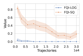
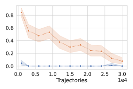
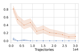
Figure 1: The value of the policy learned by FQI as a function of the size of batch dataset. The result are averaged over $90$ independently collected datasets. The figures on the left, middle and right are generated using batch data that contain only $1$, $5$, and $30$ successful trajectories respectively. The standard error of the mean is report via the shaded region.

We first evaluate FQI-log and FQI-sq on an episodic sparse cost variant of Mountain Car (Moore, 1990), where the value functions are indexed by the timestep, i.e. $v_{h}$. This environment consists of a $2$-dimensional continuous state space and $3$ discrete actions. The agent, i.e. the policy $\pi_{f_{k}}$, starts from a fixed state, $s_{1}=[-0.5,0]$, and interacts with the environment for 800 timesteps before an episode terminates. If an agent reaches the top of the hill, it remains there until the end of the episode. The cost is 0 at all timesteps except the last, when a cost of 1 is received if the agent has not reached the hilltop, and otherwise the cost is 0. A discount factor of $\gamma=1$ is used in our experiments.

We encode states as feature vectors given by the Fourier basis of order $2$ (Konidaris et al., 2011), $\phi(s)\in\mathbb{R}^{9}$, as these are known to be good features for value estimation in Mountain Car, see Chapter 9 of Sutton and Barto (2018). Given these features our function class $\mathcal{F}$ for this environment is

$$\left\{f_{h}:\mathcal{S}\times\mathcal{A}\rightarrow[0,1]:\exists\theta_{a}^{h}\ \text{ s.t. }\ f_{h}(s,a)=\sigma\left\langle\phi(s),\,\theta_{a}^{h}\right\rangle\right\},$$

where $\sigma(x)=(1+\exp(-x))^{-1}$ is the sigmoid function and $h\in[800]$. We employ the BFGS method, a quasi-Newton method with no learning rate, to find the minimizer of the losses. For strongly-convex functions, BFGS is known to converge to the global minimum superlinearly (Dennis and Moré, 1974). Finally, each batch dataset is constructed from a set of trajectories collected by running the uniform random policy from the initial state $30,000$ times. We use rejection sampling in order to guarantee each dataset has $[1,5,30]$ trajectories that reach the top of the hill. We train both FQI-log and FQI-sq on the same batch datasets with the first $n=[1,3,6,9,12,15,18,21,24,27,30]\times 10^{3}$ trajectories in order to study the relationship between the size of the batch dataset and the quality of the policies learned by FQI-log and FQI-sq. We move the successful trajectories to the front of the batch dataset so that they are included for all values of $n$.

Since BFGS does not require tuning and the same batch datasets are given to FQI-log and FQI-sq, the only variable effecting the performance of the two methods is the loss being minimized. As shown in Fig. 1, FQI-log accumulates much smaller cost then FQI-sq using fewer samples, irrespective of the number of trajectories that reach the top of the hill. FQI-log is also able to learn a near-optimal policy with only a single successful trajectory. In batch RL collecting good trajectories is often expensive, so making efficient use of the few that appear in the batch dataset is an attractive algorithmic feature. As the number of trajectories that reach the top of the hill increases, so too does the performance of FQI-sq. Since the optimal value on this problem is zero, FQI-log is able to learn a near-optimal policy using fewer samples than FQI-sq.

5.3 Asterix and Seaquest

We evaluate the deep RL variants of FQI-log and FQI-sq on the Atari 2600 games Asterix and Seaquest (Bellemare et al., 2013), and use the distributional RL algorithm C51 as an additional baseline. We adopt the data and experimental setup of Agarwal et al. (2020). The data consist of five batch datasets for each game, which were collected from independent training runs of a DQN agent (Mnih et al., 2015). Specifically, each batch dataset contains every fourth frame from 200 million frames of training; a frame skip of four and sticky actions (Machado et al., 2018) were used, whereby all actions were repeated four times consecutively and an agent randomly repeated its previous action with probability 0.25.

When the function class $\mathcal{F}$ of FQI-sq is given by a parameterized deep neural network, the algorithm is called DQN. To adapt FQI-log to the deep RL setting, we must switch the training loss from $\ell_{\text{sq}}$ to $\ell_{\log}$, and add a sigmoid activation layer to squash the output range to [0,1]. We henceforth refer to these algorithms as DQN-sq and DQN-log, respectively.

The first algorithm to implement a variant of a DQN trained with a form of log-loss is the distributional RL algorithm C51, i.e. categorical DQN (Bellemare et al., 2017). C51 minimizes the categorical log-loss across $N$ categories:

$$\ell_{\log,N}(y;\tilde{y})=\sum_{i=1}^{N}\ell_{\log}(y_{i};\tilde{y}_{i})\,,$$

for $y,\tilde{y}\in[0,1]^{N}$. C51 modifies DQN-sq in the following five ways:

1. C51 categorizes the return, i.e. sum of discounted rewards, into 51 “bins”, and predicts the probability that the outcome of a state-action pair will fall into each bin, whereas DQN-sq regresses directly on the returns.

2. C51 applies a softmax activation to its output, to normalize the values into a probability distribution over bins, as necessitated by Item S.1.

3. C51 exchanges $\ell_{\text{sq}}$ for $\ell_{\log,N}$ as the training loss.

4. C51 “clips” the targets to the finite interval $[V_{\min},V_{\max}]$, to enable mapping them into a finite set of bins.

5. C51 replaces the Bellman optimality operator $\mathcal{T}$ with a modified “distributional Bellman operator” for the updates.

For our experiments we clip the targets of DQN-log in the same way as C51, and we set $V_{\min}=0$ and $V_{\max}=10$. Since the sigmoid activation of DQN-log is a specialization of the softmax activation to the binary case, DQN-log implements the changes S.3, S.2, and S.4 to the standard form of DQN-sq. Clipping the targets introduces a bias which we correct for by similarly clipping the targets of DQN-sq. Thus our benchmark results for DQN-sq include the change S.4. Clipping the targets of DQN-sq is novel to this work and improves performance, yielding a stronger baseline. We include a comparison with the traditional unclipped version of DQN-sq in Appendix C.

Agarwal et al. (2020) found that C51 significantly outperforms DQN-sq on the games Asterix and Seaquest. We selected these games to test our hypothesis that the improved performance of C51 can be, in part, attributed to the choice of loss function. In our implementations of DQN-log and DQN-sq, we use the same hyperparameters reported by Agarwal et al. (2020). Fig. 2 shows the undiscounted return as a function of the number of training epochs. On Seaquest, DQN-log outperforms DQN-sq and is able to match the performance of C51. In Asterix, DQN-log performs similarly to DQN-sq and both achieve lower return than C51.

5.4 Experimental Findings

Our experimental results suggest that log-loss offers improvements over squared loss, as demonstrated by the results of FQI-log on Mountain Car and DQN-log on Seaquest. Furthermore, the deep RL experiments show that DQN-log can sometimes even perform similarly to the strong distributional baseline of C51. These improvements are gained by simply modifying a few lines of code, whereas C51’s implementation is much more complex.

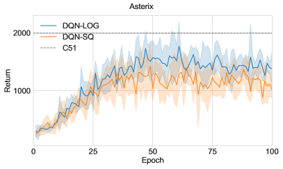
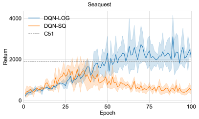
Figure 2: Learning curves on Asterix and Seaquest. The result are averaged over 5 datasets. The shaded regions represent one standard error of the mean. One epoch contains 100k updates.

6 Related Works

First-order bounds in RL

Wang et al. (2023) obtain small-cost bounds for finite-horizon batch RL problems under the distributional Bellman completeness assumption, which is stronger than the one made in Assumption 4.5. And, Wang et al., 2024 refines the bounds of Wang et al., 2023, showing second-order bounds (depending on variance) for the same algorithm proposed in the latter. They attribute their small-cost bound to the use of the distributional Bellman operator (Bellemare et al., 2023). However, their proof techniques only make use of pessimism (Buckman et al., 2021; Jin et al., 2021) and log-loss in achieving their small-cost bound. The use of pessimism is necessary for their proof in order to control the errors accumulated by use of the distribution Bellman operator during value iteration. We improve upon their work by proposing an efficient algorithm for batch RL that enjoys a similar small-cost bound without use of the distributional Bellman operator or pessimism under a weaker completeness assumption.

Jin et al. (2020a) and Wagenmaker et al. (2022) obtain regret bounds that scale with the value of the optimal policy. However in their setting, the goal is to maximize reward. Therefore, their bounds only improve upon the previous bounds (Azar et al., 2017; Yang and Wang, 2019; Jin et al., 2020b) when the optimal policy accumulates very little reward. These bounds are somewhat vacuous as they only imply that regret is low when the value of the initial policy is already close to the value of the optimal policy, both of which are close to zero. Small-cost bounds give the same rates as small-return bounds, however, they are more attractive as the cost of the initial policy can be high while the cost of the optimal policy can be low. Small-cost bounds for tabular MDPs where given by Lee et al. (2020) and for linear quadratic regulators (LQR) by Kakade et al. (2020). To our knowledge we give the first small-cost bound for batch RL under the standard completeness assumption (Antos et al., 2007; Munos and Szepesvári, 2008).

Small-cost bounds in bandits

Several works get small-cost bounds in contextual bandits (Allen-Zhu et al., 2018; Foster and Krishnamurthy, 2021; Olkhovskaya et al., 2023). Foster and Krishnamurthy (2021) show that for cost sensitive classification, a batch variant of contextual bandits, learning a value function via log-loss enjoys a small-cost bound, see Theorem 3. Whereas learning a value function via squared loss fails to achieve a small-cost guarantee, see Theorem 2. Our main result, Theorem 4.7 can be viewed as the sequel to Theorem 3 of Foster and Krishnamurthy (2021).

Abeille et al. (2021) show that for stochastic logistic bandits, where the costs/rewards are Bernoulli, the bounds scale with the variance of the optimal arm. This is simultaneously a small-cost and small-return bound. They achieve this bound by computing an optimistic estimate of the Bernoulli maximum likelihood estimator (MLE). Janz et al. (2023) extend this result and shows that for any “self-concordant” random variable computing the MLE and being optimistic gives a bound that scales with the variance of the optimal arm.

Theory on batch RL

The theoretical literature on batch RL has largely been focused on proving sample efficiency rates. Chen and Jiang (2019) proved that FQI-sq gets a rate optimal bound of $1/\sqrt{n}$ when realizability, concentrability and completeness hold. Foster et al. (2021) then show that if one assumes concentrability then completeness is a necessary assumption for sample efficient batch RL. Xie and Jiang (2021) prove that if one uses the stronger notation of concentrability from Munos (2003) then sample efficient batch RL is possible with only the added assumption of realizability, i.e. the optimal value function lies in the function class. To our knowledge the previous theoretical works on batch RL has largely focused on algorithms optimized via squared loss (Antos et al., 2007; Farahmand, 2011; Pires and Szepesvári, 2012; Chen and Jiang, 2019; Xie and Jiang, 2021).

7 Conclusions

We showed that in batch RL the loss function genuinely matters. We proved that FQI-log is more sample efficient on MDPs where the optimal cost $\bar{v}^{\star}$ is small. FQI-log is the first efficient batch RL algorithm to get a small-cost bound.

We believe our result holds generally and can be extended to any batch RL setting where the squared loss has bounded error. An intriguing extension would be deriving small-cost bounds in batch RL with only realizability (and a stronger concentrability assumption). Xie and Jiang (2021) show that with only a realizable function class squared loss gets bounded error and we conjecture a small-cost bound could be shown by adapting the analysis detailed in our work to their setting.

Wagenmaker et al. (2022) get small-return bounds for online RL in linear MDPs (Jin et al., 2020b). Another interesting avenue for future work would be getting small-cost bounds in online RL with linear function approximation. Finally, our Mountain Car experiments indicate log-loss might perform well in goal-oriented MDPs (Bertsekas, 1995). In goal-oriented MDPs the agent is tasked with reaching a goal as quickly as possible. While our Mountain Car experiments show that FQI-log is able to achieve the goal of reaching the top of the hill before the episode terminates, FQI-log does not attempt to minimize the steps needed to reach the goal. We leave the issue of reaching goals quickly as a promising direction for future research.

Appendix

Appendix A Preliminary results

In this section we introduce and prove some elementary inequalities connecting various metrics defined for nonnegative valued functions and a concentration result for the log-loss estimator taken from Foster and Krishnamurthy [2021], The concentration result gives a high probability upper bound on the error of the log-loss estimator, where the error is measured with the integrated binary Hellinger loss (to be defined below). We will base our analysis on this result. The elementary inequalities connect the integrated binary Hellinger loss to both the Hellinger distance and the so-called triangular discrimination metric, and they will allow us to reduce the analysis of our algorithm to studying the approximation error of the value functions constructed by our algorithm.

The concentration The analysis of the algorithm revolves around using the Hellinger distance, which is a distance between nonnegative valued functions. In particular, for $f,g\geq 0$ with measurable domain $\mathcal{X}$ and a measure $\lambda$ over $\mathcal{X}$, the Hellinger distance between $f$ and $g$ is defined as

$$\operatorname{H}(f,g)=\frac{1}{2}\|\sqrt{f}-\sqrt{g}\|_{2,\lambda}\,.$$

As it turns out, a version of the Hellinger distance the log-loss estimator is best

A.1 Some basic inequalities

We start by defining what we call the binary Hellinger loss between two real numbers in the $[0,1]$ interval. size=,color=red!20!white,]Cs: so maybe this should have been $\ell_{\operatorname{H}}(p,q)$. In particular, we let $p,q\in[0,1]$ reals, let

$$\operatorname{h}^{2}(p\,\|\,q):=\frac{1}{2}\left(\sqrt{p}-\sqrt{q}\right)^{2}+\frac{1}{2}\left(\sqrt{1-p}-\sqrt{1-q}\right)^{2}\,.$$ (6)

Note that the Hellinger distance between two distributions $P$ and $Q$ over a common domain is defined as $\frac{1}{\sqrt{2}}\left\|\sqrt{p}-\sqrt{q}\right\|_{2,\lambda}$, where $p=dP/d\lambda$ and $q=dQ/d\lambda$ with $\lambda$ a distribution that is dominating both $P$ and $Q$ (thus, above, $p$ ($q)$ is the density of $P$ ($Q$) relative to $\lambda$, respectively). size=,color=red!20!white,]Cs: citation With this we can note that the binary Hellinger loss between $p$ and $q$ is the Hellinger distance between the Bernoulli distributions with means $p$ and $q$. Note that $0\leq\operatorname{h}^{2}(p\mathrel{\|}q)\leq 1$.

Lemma A.1.

For all $p,q\in[0,1]$, we have

$$\frac{1}{4}\frac{(p-q)^{2}}{p+q}\leq\frac{1}{2}\left(\sqrt{p}-\sqrt{q}\right)^{2}\leq\operatorname{h}^{2}(p\,\|\,q)\,,$$ (7)

where for $p=q=0$ we define the left-hand side to be zero.

Proof.

For the first inequality in the statement, notice that

$$\frac{(p-q)^{2}}{4(p+q)}\leq\frac{(p-q)^{2}}{2(\sqrt{p}+\sqrt{q})^{2}}=\frac{1}{2}\left(\sqrt{p}-\sqrt{q}\right)^{2}\,,$$ (8)

where the inequality uses $(\sqrt{p}+\sqrt{q})^{2}\leq 2p+2q$. For the second inequality in the statement, we have

$$\frac{1}{2}\left(\sqrt{p}-\sqrt{q}\right)^{2}\leq\frac{1}{2}\left(\sqrt{p}-\sqrt{q}\right)^{2}+\frac{1}{2}\left(\sqrt{1-p}-\sqrt{1-q}\right)^{2}=\operatorname{h}^{2}(p\,\|\,q)\,.\qed$$

To state the next result, which is a simple corollary of the above inequality, we extend the definition of $\operatorname{h}^{2}$ so that it can be applied to function $f,g:\mathcal{X}\to[0,1]$. In particular, we let $\operatorname{h}^{2}(f,g):\mathcal{X}\to[0,1]$ defined via size=,color=red!20!white,]Cs: so maybe this should have been $\ell_{\operatorname{H}}(f,g,\cdot)$. Oh well..

$$(\operatorname{h}^{2}(f,g))(x)=\operatorname{h}^{2}(f(x)\mathrel{\|}g(x))\,\qquad x\in\mathcal{X}\,.$$

With this, a simple corollary of the first statement of this section is as follows:

Corollary A.2.

For any distribution $\nu$ over the set $\mathcal{X}$ and any measurable functions $f,g:\mathcal{X}\to[0,1]$,

$$\left\|\frac{f-g}{\sqrt{f+g}}\right\|_{2,\nu}\leq\sqrt{2}\left\|\sqrt{f}-\sqrt{g}\right\|_{2,\nu}\leq 2\left\|\operatorname{h}^{2}(f,g)\right\|_{1,\nu}^{1/2}\,.$$

where for $f(x)=g(x)=0$, we define $\frac{f(x)-g(x)}{\sqrt{f(x)+g(x)}}=0$.

We call the quantity on the right-hand side as the square root of the integrated binary Hellinger loss between $f$ and $g$. Squaring all quantities above, we get the equivalent inequalities

$$\frac{1}{4}\left\|\frac{f-g}{\sqrt{f+g}}\right\|^{2}_{2,\nu}\leq\frac{1}{2}\left\|\sqrt{f}-\sqrt{g}\right\|^{2}_{2,\nu}\leq\left\|\operatorname{h}^{2}(f,g)\right\|_{1,\nu}\,.$$

With words, this states, that the integrated binary Hellinger loss between $f$ and $g$ is lower bounded by their squared Hellinger distance, which is lower bounded, up to a constant factor, by the so-called triangular discrimination distance them. The latter is in essence the squared distance between $f$ and $g$, where their pointwise differences is rescaled with the square root of the sum between the functions. Because $|a-b|/\sqrt{a+b}\leq\varepsilon$ implies $|a-b|\leq\varepsilon\sqrt{a+b}\leq\varepsilon\max(\sqrt{a},\sqrt{b})$, we see that a bound on the rescaled distance between two values tightens the bound between them when both values are close to zero. In essence, this is what will take advantage of later in our analysis.

Proof.

Apply Lemma A.1 pointwise and then integrate both sides of the inequality over $\nu$, and then take the square root and simplify the constants. ∎

A.2 Concentration for the log-loss estimator

Fix a set $\mathcal{X}$, which, for the sake of avoiding measurability issues is assumed to be finite. Let $(X_{1},Y_{1}),\dots,(X_{n},Y_{n})$ independent, identically distributed random variables taking values in $\mathcal{X}\times[0,1]$. Let $f^{\star}$ be the regression function underlying $\nu$: $f^{\star}(x)=\mathbb{E}\,\left[Y_{1}\,|\,X_{1}=x\right]$. Let $\mathcal{F}\subset\{f\,:\,f:\mathcal{X}\to[0,1]\}$ be a finite set of $[0,1]$-valued functions with domain $\mathcal{X}$. Recall the log-loss estimator:

$$\hat{f}_{\log}=\mathop{\rm arg\,min}_{f\in\mathcal{F}}\sum_{i=1}^{n}\ell_{\log}(f(X_{i});\,Y_{i}),$$

where, for $y,y^{\prime}\in[0,1]$, size=,color=red!20!white,]Cs: what happens at the boundary!? size=,color=green!20!white,]AA: Not sure this was the setting in Dylan’s theorem? size=,color=red!20!white,]Cs: my question was rhetoric. I mean, the reader needs to be told what happens and you need to know.. Hint: we need to say that we let $0\log\infty=\lim_{x\to 0}x\log 1/x=0$. I am just saying in general be careful so that whatever you write is well-defined. size=,color=red!20!white,]Cs: note that we need $y\in[0,1]$, but strictly speaking, $y^{\prime}$ could take any value. this allows the targets $Y_{i}$ to lie outside of the $[0,1]$ range..

$$\ell_{\log}(y;\,y^{\prime}):=y^{\prime}\log\frac{1}{y}+(1-y^{\prime})\log\frac{1}{1-y}\,,$$

where we define $0\log\infty=\lim_{x\to 0}x\log 1/x=0$. Foster and Krishnamurthy [2021] show the following concentration result for $\hat{f}_{\log}$, which we will need:

Theorem A.3.

Suppose $f^{\star}\in\mathcal{F}$. Let $D_{n}=((X_{1},Y_{1}),\dots,(X_{n},Y_{n}))$. Then, for any $\delta\in(0,1)$, with probability at least $1-\delta$, we have

$$\|\operatorname{h}^{2}(\hat{f}_{\log},f^{\star})\|_{1,\nu}\leq\frac{2\log(|\mathcal{F}|/\delta)}{n}\,,$$

where $\nu$ denotes the common distribution over $X_{1},\dots,X_{n}$.

Proof.

The result follows from the last equation on page 24 of the arXiv version of the paper by Foster and Krishnamurthy [2021] with $A=1$. ∎

Appendix B Proof of Theorem 4.7

In this section we give the main steps of the proof of Theorem 4.7. For the benefit of the reader, we first reproduce the text of the theorem:

Theorem B.1.

Given a dataset $D=\{(S_{i},A_{i},C_{i},S_{i}^{\prime})\}_{i=1}^{n}$ with $n\in\mathbb{N}$ and a finite function class $\mathcal{F}\subseteq(\mathcal{S}\times\mathcal{A}\rightarrow[0,1])$ that satisfy Assumptions 4.2, 4.3, 4.5 and 4.6, $B=1$, it holds with probability $1-\delta$, the output policy of FQI-log after $k$ iterations, $\pi_{k}=\pi_{f_{k}}$, satisfies

$$\bar{v}^{\pi_{k}}-\bar{v}^{\star}\leq\tilde{C}\left(\frac{1}{(1-\gamma)^{2}}\sqrt{\frac{\bar{v}^{\star}C\log\left(\lvert\mathcal{F}\rvert^{2}/\delta\right)}{n}}+\frac{C\log\left(\lvert\mathcal{F}\rvert^{2}/\delta\right)}{(1-\gamma)^{4}n}+\frac{\gamma^{\frac{k}{2}}}{1-\gamma}+\frac{\gamma^{k}}{(1-\gamma)^{2}}\right)\,.$$ (9)

where $\tilde{C}>0$ is an absolute constant.

The proof is reduced to two propositions and some extra calculations. We start by stating the two propositions first. The proofs of these propositions require more steps and will be developed in their own sections, following the proof of the main result, which ends this section.

The first proposition shows that the error of a policy that is greedy with respect to an action-value function $f:\mathcal{S}\times\mathcal{A}\to[0,\infty)$ can be bounded by the triangular discrimination distance between the action-value function and $q^{*}$, the optimal action-value function in our MDP. To state this proposition, for $f$ as above we define $\Delta_{f}:\mathcal{S}\times\mathcal{A}\to[0,\infty)$, as the pointwise triangular deviation of $f$ from $q^{*}$:

$$\Delta_{f}(s,a)=\frac{f(s,a)-q^{\star}(s,a)}{\sqrt{f(s,a)+q^{\star}(s,a)}}\,,\qquad\qquad(s,a)\in\mathcal{S}\times\mathcal{A}\,.$$

To state the proposition, recall that for a distribution $\eta$ over the states and for a stationary policy $\pi$, we let $\eta\times\pi$ denote the joint probability distribution over the state-action pairs resulting from first sampling a state $S$ from $\eta$, followed by choosing an action $A$ at random from $\pi(S)$. size=,color=red!20!white,]Cs: review notation/terminology for policies. also, this is just applying a Markov kernel.. Same as $\nu P$. So why the $\times$? With this, the first proposition is as follows:

Proposition B.2.

Let $f:\mathcal{S}\times\mathcal{A}\rightarrow[0,\infty)$ and let $\pi=\pi_{f}$ be a policy that is greedy with respect to $f$. Define $D_{f}=\sup_{h\geq 1}\max(\left\|\Delta_{f}\right\|_{2,\eta_{h}^{\pi}\times\pi},\left\|\Delta_{f}\right\|_{2,\eta_{h}^{\pi}\times\pi^{\star}})$. Then, it holds that

$$\bar{v}^{\pi}-\bar{v}^{\star}\leq\frac{22D_{f}}{1-\gamma}\sqrt{2\bar{v}^{\star}}+\frac{512D_{f}^{2}}{(1-\gamma)^{2}}\,.$$

Recall that above $\eta_{h}^{\pi}$ is the distribution induced over the states in step $h$ when $\pi$ is followed from the start state distribution $\eta_{1}$. As expected, the proof uses the performance difference lemma, followed by arguments that relate the stage-wise expected error that arises from the performance difference lemma to the “size” of $\Delta_{f}$.

When the above proposition is applied to $f=f_{k}$, the action-value function obtained in the $k$th iteration of our algorithm, we see that it remains to bound $D_{f_{k}}$. The bound will be based on the second proposition:

Proposition B.3.

For any admissible distribution $\nu$ over $\mathcal{S}\times\mathcal{A}$ that may also depend on the data $D_{n}$,size=,color=red!20!white,]Cs: I commented out the assumptions.. Usually one says before the lemmas that the assumptions hold.. for any $0<\delta<1$, $k\geq 1$, with probability $1-\delta$,

$$\left\|\Delta_{f_{k}}\right\|_{2,\nu}\leq\sqrt{\frac{32C\log\left(\lvert\mathcal{F}\rvert^{2}/\delta\right)}{(1-\gamma)^{2}n}}+\sqrt{2}\gamma^{\frac{k}{2}}\,,$$ (10)

where $f_{k}$ denotes the value function computed by FQI, Algorithm 1, in step $k$ based on the data $D_{n}$.

The proof of this proposition uses (i) showing that $\mathcal{T}$ enjoys some contraction properties with respect to appropriately chosen Hellinger distances; (ii) using these contraction properties to show that the Hellinger distance between $f_{k}$ and $q^{*}$ is controlled by the Hellinger distances between $f_{k}$ and $\mathcal{T}f_{k}$, and then using the results of the previous section to show that these are controlled by the algorithm.

With these two statements in place, the proof the main theorem is as follows:

Proof of Theorem B.1.

Fix $k\geq 1$. For $h\geq 1$, let $\eta_{h}^{k}=\eta_{h}^{\pi_{k}}$, $D_{f_{k}}=\sup_{h\geq 1}\max(\left\|\Delta_{f_{k}}\right\|_{2,\eta_{h}^{k}\times\pi_{k}},\left\|\Delta_{f_{k}}\right\|_{2,\eta_{h}^{k}\times\pi^{\star}})$. Since, by definition, $\pi_{k}$ is greedy with respect to $f_{k}$, we can use Proposition B.2 to get

$$\bar{v}^{\pi_{k}}-\bar{v}^{\star} \leq\frac{22\sqrt{2}D_{f_{k}}}{1-\gamma}\sqrt{\bar{v}^{\star}}+\frac{512D_{f_{k}}^{2}}{(1-\gamma)^{2}}\,.$$ (11)

It remains to bound $D_{f_{k}}$. An application of Proposition B.3 gives that for any $0<\delta<1$, with probability $1-\delta$,

$$S:=\sup_{\nu\textrm{ admissible}}\left\|D_{f_{k}}\right\|_{2,\nu}\leq\sqrt{\frac{32C\log\left(\lvert\mathcal{F}\rvert^{2}/\delta\right)}{(1-\gamma)^{2}n}}+\sqrt{2}\gamma^{\frac{k}{2}}\,.$$ (12)

Since $\eta_{h}^{k}\times\pi_{k}$ and $\eta_{h}^{k}\times\pi^{\star}$ are admissible, as can be easily seen with an argument similar to that used in the proof of Lemma B.16, it follows that with probability $1-\delta$,

$$D_{f_{k}}\leq S\leq\sqrt{\frac{32C\log\left(\lvert\mathcal{F}\rvert^{2}/\delta\right)}{(1-\gamma)^{2}n}}+\sqrt{2}\gamma^{\frac{k}{2}}\,.$$ (13)

Squaring both sides and using the inequality $(a+b)^{2}\leq 2a^{2}+2b^{2}$, we get that the inequality

$$D_{f_{k}}^{2}\leq\frac{64C\log\left(\lvert\mathcal{F}\rvert^{2}/\delta\right)}{(1-\gamma)^{2}n}+4\gamma^{k}$$

also holds, on the same event when Eq. 13 holds. Plugging these bounds into Eq. 11, we get that with probability at least $1-\delta$,

$$\bar{v}^{\pi_{k}}-\bar{v}^{\star} \leq\frac{22\sqrt{2}D_{f_{k}}}{1-\gamma}\sqrt{\bar{v}^{\star}}+\frac{512D_{f_{k}}^{2}}{(1-\gamma)^{2}}$$

$$\leq\frac{176}{(1-\gamma)^{2}}\sqrt{\frac{\bar{v}^{\star}C\log\left(\lvert\mathcal{F}\rvert^{2}/\delta\right)}{n}}+\frac{32768C\log\left(\lvert\mathcal{F}\rvert^{2}/\delta\right)}{(1-\gamma)^{4}n}+\frac{44\gamma^{\frac{k}{2}}}{1-\gamma}+\frac{2048\gamma^{k}}{(1-\gamma)^{2}}\,.\qed$$

B.1 An error bound for greedy policies: Proof of Proposition B.2

The analysis in this section is inspired by the proof of Lemma 1 of Foster and Krishnamurthy [2021]. We deviate from their analysis to avoid introducing an extra $|\mathcal{A}|$ factor in the bounds.

Additional Notations

For any function $g:\mathcal{S}\times\mathcal{A}\rightarrow\mathbb{R}$ and policy $\pi$, define $g(s,\pi)=\sum_{a\in\mathcal{A}}\pi(a|s)g(s,a)$. For any $\nu\in\mathcal{M}_{1}(S\times A)$ which is an $|\mathcal{S}\times\mathcal{A}|$ dimensional row vector, define $\nu P\in\mathcal{M}_{1}(\mathcal{S})$ as the distribution obtained over the states by first sampling a state-action pair from $\nu$ and then following $P$. That is, $\nu P$ is the distribution of $S^{\prime}\sim P(\cdot|S,A)$ where $(S,A)\sim\nu$. size=,color=red!20!white,]Cs: This should be $\nu P$. The standard convention is to think of distributions as row vectors. A probability kernel, such as $P$, is a matrix of appropriate size. Then $\nu P$ gives a row vector, with the usual vector-matrix multiplication rules, which is exactly what we want here. We can think of $\nu P$ as the distribution we get when $P$ is composed with $\nu$. For any function $f:\mathcal{S}\times\mathcal{A}\rightarrow[0,\infty)$, in addition to $\Delta_{f}$, we also define $\xi_{f}:\mathcal{S}\times\mathcal{A}\to\mathbb{R}$ as

$$\xi_{f}(s,a)=f(s,a)+q^{\star}(s,a)\,,\qquad\qquad(s,a)\in\mathcal{S}\times\mathcal{A}\,.$$ (14)

Recall that $\mathcal{F}$ contains $[0,1]$-valued functions with domain $\mathcal{S}\times\mathcal{A}$ and as such for any $f\in\mathcal{F}$, $\Delta_{f}$ and $\xi_{f}$ are well-defined.

We start with the performance difference lemma, which is stated without a proof:

Lemma B.4 (Performance Difference Lemma of Kakade and Langford).

For policies $\pi,\bar{\pi}:\mathcal{S}\rightarrow\mathcal{M}_{1}(\mathcal{A})$, we have

$$\bar{v}^{\pi}-\bar{v}^{\bar{\pi}}=\sum_{h=1}^{\infty}\gamma^{h-1}\left\langle\eta_{h}^{\pi},\,q^{\bar{\pi}}(\cdot,\pi)-v^{\bar{\pi}}\right\rangle\,.$$ (15)

Proof.

See Lemma 6.1 by Kakade and Langford [2002]. ∎

The next lemma upper bounds the one-norm distance between a nonnegative-valued function $f:\mathcal{S}\times\mathcal{A}\to[0,\infty)$ and $q^{*}$ in terms of appropriate norms of $\Delta_{f}$ and $\xi_{f}$.

Lemma B.5.

For any function $f:\mathcal{S}\times\mathcal{A}\to[0,\infty)$ and distribution $\nu\in\mathcal{M}_{1}(S\times A)$, we have

$$\lVert f-q^{\star}\rVert_{1,\nu}\leq\lVert\xi_{f}\rVert_{1,\nu}^{1/2}\cdot\lVert\Delta_{f}\rVert_{2,\nu}\,.$$ (16)

Proof.

We have

$$\lVert f-q^{\star}\rVert_{1,\nu} =\left\|\sqrt{f+q^{\star}}\cdot\frac{f-q^{\star}}{\sqrt{f+q^{\star}}}\right\|_{1,\nu}$$ (17)

$$\leq\left\|f+q^{\star}\right\|_{1,\nu}^{1/2}\cdot\left\|\frac{(f-q^{\star})^{2}}{f+q^{\star}}\right\|_{1,\nu}^{1/2}$$ (Cauchy-Schwarz)

$$=\left\|\xi_{f}\right\|_{1,\nu}^{1/2}\cdot\left\|\Delta_{f}\right\|_{2,\nu}\,.\qed$$ (18)

Lemma B.6.

Let $f:S\times A\rightarrow[0,\infty)$ and let $\pi=\pi_{f}$ be a policy that is greedy with respect to $f$ and $h$ be a nonnegative integer. Then it holds that size=,color=red!20!white,]Cs: why use $\tilde{\pi}$. why not simply use $\pi$? less clutter is good on the eyes.

$$\langle\eta_{h}^{\pi},\,q^{\star}(\cdot,\pi)-v^{\star}\rangle\leq\left(\left\|\xi_{f}\right\|_{1,\eta_{h}^{\pi}\times\pi}^{1/2}+\left\|\xi_{f}\right\|_{1,\eta_{h}^{\pi}\times\pi^{\star}}^{1/2}\right)\left(\left\|\Delta_{f}\right\|_{2,\eta_{h}^{\pi}\times\pi}+\left\|\Delta_{f}\right\|_{2,\eta_{h}^{\pi}\times\pi^{\star}}\right)\,.$$

Proof.

We have

$$\left\langle\eta_{h}^{\pi},\,q^{\star}(\cdot,\pi)-v^{\star}\right\rangle =\left\langle\eta_{h}^{\pi},\,q^{\star}(\cdot,\pi)-q^{\star}(\cdot,\pi^{\star})\right\rangle v^{\star}$$ (Defn of )

$$\leq\left\langle\eta_{h}^{\pi},\,q^{\star}(\cdot,\pi)-f(\cdot,\pi)+f(\cdot,\pi^{\star})-q^{\star}(\cdot,\pi^{\star})\right\rangle f(\cdot,\pi)\leq f(\cdot,\pi^{\star}) \pi$$ ( by defn of )

$$\leq\left\|q^{\star}-f\right\|_{1,\eta_{h}^{\pi}\times\pi}+\left\|f-q^{\star}\right\|_{1,\eta_{h}^{\pi}\times\pi^{\star}}\,.$$ (triangle inequality)

size=,color=red!20!white,inline]Cs: (defn of $v^{\star}$ or properties of $v^{\star}/q^{\star}$. By the way, these should be mentioned upfront! Maybe in the notation section and we can refer back to there. Now,

$$\left\|q^{\star}-f\right\|_{1,\eta_{h}^{\tilde{\pi}}\times\tilde{\pi}}+\left\|f-q^{\star}\right\|_{1,\eta_{h}^{\tilde{\pi}}\times\pi^{\star}}$$

$$\leq\left\|\xi_{f}\right\|_{1,\eta_{h}^{\tilde{\pi}}\times\tilde{\pi}}^{1/2}\cdot\left\|\Delta_{f}\right\|_{2,\eta_{h}^{\tilde{\pi}}\times\tilde{\pi}}+\left\|\xi_{f}\right\|_{1,\eta_{h}^{\tilde{\pi}}\times\pi^{\star}}^{1/2}\cdot\left\|\Delta_{f}\right\|_{2,\eta_{h}^{\tilde{\pi}}\times\pi^{\star}}$$ (Lemma B.5)

$$\leq\left(\left\|\xi_{f}\right\|_{1,\eta_{h}^{\tilde{\pi}}\times\tilde{\pi}}^{1/2}+\left\|\xi_{f}\right\|_{1,\eta_{h}^{\tilde{\pi}}\times\pi^{\star}}^{1/2}\right)\left(\left\|\Delta_{f}\right\|_{2,\eta_{h}^{\tilde{\pi}}\times\tilde{\pi}}+\left\|\Delta_{f}\right\|_{2,\eta_{h}^{\tilde{\pi}}\times\pi^{\star}}\right)\,.\qed$$

Lemma B.7.

For any function $f:\mathcal{S}\times\mathcal{A}\rightarrow[0,\infty)$ and distribution $\nu\in\mathcal{M}_{1}(\mathcal{S}\times\mathcal{A})$, it holds that size=,color=red!20!white,]Cs: where is admissibility used? I got rid of it. It was not used. In general, one should eliminate conditions not used.

$$\left\|f+q^{\star}\right\|_{1,\nu}\leq 4\left\|q^{\star}\right\|_{1,\nu}+\left\|\Delta_{f}\right\|_{2,\nu}^{2}\,.$$ (19)

Proof.

Let $f\in\mathcal{F}$ be fixed, we have

$$\left\|f+q^{\star}\right\|_{1,\nu} =\left\|f-q^{\star}+q^{\star}+q^{\star}\right\|_{1,\nu}$$

$$\leq 2\left\|q^{\star}\right\|_{1,\nu}+\left\|f-q^{\star}\right\|_{1,\nu}$$ (triangle inequality)

$$=2\left\|q^{\star}\right\|_{1,\nu}+\left\|\sqrt{f+q^{\star}}\,\frac{f-q^{\star}}{\sqrt{f+q^{\star}}}\right\|_{1,\nu}$$

$$\leq 2\left\|q^{\star}\right\|_{1,\nu}+\frac{1}{2}\left\|f+q^{\star}+\frac{(f-q^{\star})^{2}}{f+q^{\star}}\right\|_{1,\nu} ab\leq\tfrac{a^{2}+b^{2}}{2} a,b$$ ( for nonnegative reals)

$$\leq 2\left\|q^{\star}\right\|_{1,\nu}+\frac{1}{2}\left\|f+q^{\star}\right\|_{1,\nu}+\frac{1}{2}\left\|\Delta_{f}\right\|_{2,\nu}^{2}\,.$$ (triangle inequality)

Rearranging and multiplying through by two gives the statement. ∎

Lemma B.8.

Let $f:\mathcal{S}\times\mathcal{A}\rightarrow[0,\infty)$ and let $\pi=\pi_{f}$ be a policy that is greedy with respect to $f$. Define $D_{f}=\sup_{h\geq 1}\max(\left\|\Delta_{f}\right\|_{2,\eta_{h}^{\pi}\times\pi},\left\|\Delta_{f}\right\|_{2,\eta_{h}^{\pi}\times\pi^{\star}})$. Then, it holds that

$$\bar{v}^{\pi}-\bar{v}^{\star} \leq 11D_{f}\sum_{h=1}^{\infty}\gamma^{h-1}\left\|v^{\star}\right\|_{1,\eta_{h}^{k}}^{1/2}+\frac{28D_{f}^{2}}{1-\gamma}\,.$$

Proof.

Recall that by the performance difference lemma, Lemma B.4, it holds that

$$\bar{v}^{\pi}-\bar{v}^{\star}=\sum_{h=1}^{\infty}\gamma^{h-1}\langle\eta_{h}^{\pi},\,q^{\star}(\cdot,\pi)-v^{\star}\rangle\,.$$ (20)

For the remainder of this proof we fix $h\geq 1$. For the $h^{\mathrm{th}}$ term from the above display, we have

$$\langle\eta_{h}^{\pi},\,q^{\star}(\cdot,\pi)-v^{\star}\rangle\leq\left(\left\|\xi_{f}\right\|_{1,\eta_{h}^{\pi}\times\pi}^{1/2}+\left\|\xi_{f}\right\|_{1,\eta_{h}^{\pi}\times\pi^{\star}}^{1/2}\right)\left(\left\|\Delta_{f}\right\|_{2,\eta_{h}^{\pi}\times\pi}+\left\|\Delta_{f}\right\|_{2,\eta_{h}^{\pi}\times\pi^{\star}}\right)$$ (Lemma B.6)

$$\leq\left(\sqrt{4\left\|q^{\star}\right\|_{1,\eta_{h}^{\pi}\times\pi}+\left\|\Delta_{f}\right\|_{2,\eta_{h}^{\pi}\times\pi}^{2}}+\sqrt{4\left\|q^{\star}\right\|_{1,\eta_{h}^{\pi}\times\pi^{\star}}+\left\|\Delta_{f}\right\|_{2,\eta_{h}^{\pi}\times\pi^{\star}}^{2}}\right)\left(\left\|\Delta_{f}\right\|_{2,\eta_{h}^{\pi}\times\pi}+\left\|\Delta_{f}\right\|_{2,\eta_{h}^{\pi}\times\pi^{\star}}\right)\,.$$ (Lemma B.7)

Now recall that by definition

$$\max\left\{\left\|\Delta_{f}\right\|_{2,\eta_{h}^{\pi}\times\pi},\left\|\Delta_{f}\right\|_{2,\eta_{h}^{\pi}\times\pi^{\star}}\right\}\leq D_{f}\,.$$

Hence,

$$\langle\eta_{h}^{\pi},\,q^{\star}(\cdot,\pi)-v^{\star}\rangle$$

$$\leq 2D_{f}\left(\sqrt{4\left\|q^{\star}\right\|_{1,\eta_{h}^{\pi}\times\pi}+D_{f}^{2}}+\sqrt{4\left\|q^{\star}\right\|_{1,\eta_{h}^{\pi}\times\pi^{\star}}+D_{f}^{2}}\right)$$ (21)

$$\leq 2D_{f}\left(2D_{f}+\sqrt{4\left\|q^{\star}\right\|_{1,\eta_{h}^{\pi}\times\pi}}+\sqrt{4\left\|q^{\star}\right\|_{1,\eta_{h}^{\pi}\times\pi^{\star}}}\right) \sqrt{a+b}\leq\sqrt{a}+\sqrt{b}$$ ()

$$=4D_{f}^{2}+4D_{f}\left\|q^{\star}\right\|_{1,\eta_{h}^{\pi}\times\pi}^{1/2}+4D_{f}\left\|q^{\star}\right\|_{1,\eta_{h}^{\pi}\times\pi^{\star}}^{1/2}$$

$$\leq 20D_{f}^{2}+\frac{\left\|q^{\star}\right\|_{1,\eta_{h}^{\pi}\times\pi}+\left\|q^{\star}\right\|_{1,\eta_{h}^{\pi}\times\pi^{\star}}}{2}\,. ab\leq\tfrac{a^{2}+b^{2}}{2} a,b a=4D_{f}$$ ( for nonnegative reals, twice with )

Using that $v^{\star}$, $q^{\star}$ are nonnegative valued and that $v^{\star}(\cdot)=q^{\star}(\cdot,\pi^{\star})$, we calculate $\langle\eta_{h}^{\pi},v^{\star}\rangle=\left\|v^{\star}\right\|_{1,\eta_{h}^{\pi}}=\left\|q^{\star}\right\|_{1,\eta_{h}^{\pi}\times\pi^{\star}}$. Thus, by the previous display, after rearranging, we get

$$\left\|q^{\star}\right\|_{1,\eta_{h}^{\pi}\times\pi}=\langle\eta_{h}^{\pi},\,q^{\star}(\cdot,\pi)\rangle\leq 40D_{f}^{2}+3\left\|q^{\star}\right\|_{1,\eta_{h}^{\pi}\times\pi^{\star}}\,,$$

where the equality used the non-negativity of $q^{\star}$. Plugging this back into the inequality in Section B.1 gives

$$\langle\eta_{h}^{\pi},\,q^{\star}(\cdot,\pi)-v^{\star}\rangle\leq 2D_{f}\left(\sqrt{4\left\|q^{\star}\right\|_{1,\eta_{h}^{\pi}\times\pi^{\star}}+D_{f}^{2}}+\sqrt{4\left\|q^{\star}\right\|_{1,\eta_{h}^{\pi}\times\pi}+D_{f}^{2}}\right)$$ (restating Section B.1)

$$\leq 2D_{f}\left(\sqrt{4\left\|q^{\star}\right\|_{1,\eta_{h}^{\pi}\times\pi^{\star}}+D_{f}^{2}}+\sqrt{160D_{f}^{2}+12\left\|q^{\star}\right\|_{1,\eta_{h}^{\pi}\times\pi^{\star}}+D_{f}^{2}}\right)$$

$$\leq 2D_{f}\left(2\left\|q^{\star}\right\|_{1,\eta_{h}^{\pi}\times\pi^{\star}}^{1/2}+D_{f}+\sqrt{161}D_{f}+\sqrt{12}\left\|q^{\star}\right\|_{1,\eta_{h}^{\pi}\times\pi^{\star}}^{1/2}\right) \sqrt{a+b}\leq\sqrt{a}+\sqrt{b}$$ ()

$$\leq 11D_{f}\left\|q^{\star}\right\|_{1,\eta_{h}^{\pi}\times\pi^{\star}}^{1/2}+28D_{f}^{2}\,.$$

Combining this with Eq. 20 gives the desired inequality. ∎

Lemma B.9.

For any policy $\pi:\mathcal{S}\rightarrow\mathcal{M}_{1}(\mathcal{A})$ we have

$$\sum_{h=1}^{\infty}\gamma^{h-1}\,\sqrt{\left\langle\eta_{h}^{\pi},\,v^{\pi}\right\rangle}\leq\frac{2\sqrt{\bar{v}^{\pi}}}{1-\gamma}\,.$$ (22)

Proof.

Notice that size=,color=red!20!white,]Cs: make sure $\left\langle\cdot,\,\cdot\right\rangle$ is defined. size=,color=green!20!white,]AA: It is defined in the main.

$$\bar{v}^{\pi} =\left\langle\eta_{1},\,v^{\pi}\right\rangle$$

$$=\left\langle\eta_{1}^{\pi},\,c(\cdot,\pi)\right\rangle+\gamma\left\langle\eta_{2}^{\pi},\,c(\cdot,\pi)\right\rangle+\gamma^{2}\left\langle\eta_{3}^{\pi},\,c(\cdot,\pi)\right\rangle+\dotsb+\gamma^{h-1}\left\langle\eta_{h}^{\pi},\,v^{\pi}\right\rangle$$

$$\geq\gamma^{h-1}\left\langle\eta_{h}^{\pi},\,v^{\pi}\right\rangle$$

where the inequality follows from the non-negativity of the costs. Simple rearrangement gives

$$\left\langle\eta_{h}^{\pi},\,v^{\pi}\right\rangle\leq\frac{\bar{v}^{\pi}}{\gamma^{h-1}}\,.$$

Using this inequality, we get

$$\sum_{h=1}^{\infty}\gamma^{h-1}\,\sqrt{\left\langle\eta_{h}^{\pi},\,v^{\pi}\right\rangle} \leq\sum_{h=1}^{\infty}\gamma^{h-1}\,\sqrt{\frac{\bar{v}^{\pi}}{\gamma^{h-1}}}=\sum_{h=1}^{\infty}\sqrt{\gamma^{h-1}\bar{v}^{\pi}}\leq\frac{2\sqrt{\bar{v}^{\pi}}}{1-\gamma}\,,$$

where for the last inequality we used that $1/(1-\sqrt{\gamma})\leq 2/(1-\gamma)$. ∎

With this we are ready to prove Proposition B.2:

Proof of Proposition B.2.

For $h\geq 1$, let $\eta_{h}=\eta_{h}^{\pi}$. Starting from Lemma B.8, we bound $\bar{v}^{\pi}-\bar{v}^{\star}$ as follows:

$$\bar{v}^{\pi}-\bar{v}^{\star} \leq 11D_{f}\sum_{h=1}^{\infty}\gamma^{h-1}\left\|v^{\star}\right\|_{1,\eta_{h}}^{1/2}+28D_{f}^{2}\sum_{h=1}^{\infty}\gamma^{h-1}$$ (Lemma B.8)

$$=11D_{f}\sum_{h=1}^{\infty}\gamma^{h-1}\sqrt{\left\langle\eta_{h},\,v^{\star}\right\rangle}+\frac{28D_{f}^{2}}{1-\gamma}$$

$$\leq 11D_{f}\sum_{h=1}^{\infty}\gamma^{h-1}\sqrt{\left\langle\eta_{h},\,v^{\pi}\right\rangle}+\frac{28D_{f}^{2}}{1-\gamma} v^{\star}$$ (Defn of )

$$\leq\frac{22D_{f}\sqrt{\bar{v}^{\pi}}}{1-\gamma}+\frac{28D_{f}^{2}}{1-\gamma} \qquad(\star)$$ (Lemma B.9, )

$$\leq\frac{22^{2}D_{f}^{2}}{2(1-\gamma)^{2}}+\frac{\bar{v}^{\pi}}{2}+\frac{28D_{f}^{2}}{1-\gamma}\,. ab\leq(a^{2}+b^{2})/2 a,b\geq 0$$ (, )

Rearranging the last inequality obtained, we get

$$\bar{v}^{\pi}\leq 2\bar{v}^{\star}+\frac{22^{2}D_{f}^{2}}{(1-\gamma)^{2}}+\frac{56D_{f}^{2}}{1-\gamma}\,.$$

Plugging this bound into $(\star)$, we get

$$\bar{v}^{\pi}-\bar{v}^{\star} \leq\frac{22D_{f}}{1-\gamma}\sqrt{2\bar{v}^{\star}+\frac{22^{2}D_{f}^{2}}{(1-\gamma)^{2}}+\frac{56D_{f}^{2}}{1-\gamma}}+\frac{28D_{f}^{2}}{1-\gamma}$$

$$\leq\frac{22\sqrt{2}D_{f}}{1-\gamma}\sqrt{\bar{v}^{\star}}+\frac{22^{2}D_{f}^{2}}{(1-\gamma)^{2}}+\frac{165D_{f}^{2}}{(1-\gamma)^{3/2}}+\frac{28D_{f}^{2}}{1-\gamma} \sqrt{a+b}\leq\sqrt{a}+\sqrt{b} a,b\geq 0$$ (, twice)

$$\leq\frac{22\sqrt{2}D_{f}}{1-\gamma}\sqrt{\bar{v}^{\star}}+\frac{512D_{f}^{2}}{(1-\gamma)^{2}}\,.\qed$$

B.2 Bounding the triangular deviation between $f_{k}$ and $q^{*}$: Proof of Proposition B.3

As explained earlier, the analysis in this section uses contraction arguments that have a long history in the analysis of dynamic programming algorithms in the context of MDPs. The novelty is that we need to bound the triangular deviation to $q^{*}$. As this has been shown to be upper bounded by the Hellinger distance (Corollary A.2), we switch to Hellinger distances and establishes contraction properties of $\mathcal{T}$ with respect to such distances. This required new proofs. The change of measure arguments used in the “error propagation analysis” are standard.

The following lemma, at a high level, establishes that the map $f\mapsto f^{\wedge}$ (“$\min$-operator”) is a non-expansion over the set of nonnegative functions with domain $\mathcal{S}\times\mathcal{A}$ and $\mathcal{S}$, respectively, when these function spaces are equipped with appropriate norms:

Lemma B.10.

Define the policy $\pi_{f,g}(s)=\arg\min_{a\in A}\min\{f(s,a),g(s,a)\}$ and assume that $f,g:\mathcal{S}\times\mathcal{A}\rightarrow[0,\infty)$. size=,color=red!20!white,]Cs: what happened with $\mathcal{S}$ and $\mathcal{A}$ vs. $S$ and $A$?size=,color=green!20!white,]AA: It should always be $\mathcal{S}$ and $\mathcal{A}$ my Then, for any distribution $\eta\in\mathcal{M}_{1}(\mathcal{S})$, we have that

$$\left\|\sqrt{f^{\wedge}}-\sqrt{g^{\wedge}}\right\|_{2,\eta}\leq\left\|\sqrt{f}-\sqrt{g}\right\|_{2,\eta\times\pi_{f,f^{\prime}}}\,.$$ (23)

Proof.

Notice that for two finite sets of reals, $U=\{u_{1},\dots,u_{n}\}$, $V=\{v_{1},\dots,v_{m}\}$, with $u_{1}=\min U$, $v_{j}=\min V$, $u_{1}\leq v_{j}$, $j\in[m]$, we have $|\min U-\min V|=v_{j}-u_{1}\leq v_{1}-u_{1}\leq|u_{1}-v_{1}|$. By taking the square root of all the elements in both $U$ and $V$, assuming these are nonnegative, we also get that

$$|\sqrt{\min U}-\sqrt{\min V}|\leq\sqrt{v_{1}}-\sqrt{u_{1}}\leq|\sqrt{u_{1}}-\sqrt{v_{1}}|\,.$$ (24)

Hence,

$$\left\|\sqrt{f^{\wedge}}-\sqrt{g^{\wedge}}\right\|_{2,\eta}^{2} =\sum_{s\in S}\eta(s)\left(\sqrt{\min_{a\in A}f(s,a)}-\sqrt{\min_{a\in A}g(s,a)}\right)^{2}$$

$$=\sum_{s\in S}\eta(s)\left(\sqrt{f\left(s,\pi_{f}(s)\right)}-\sqrt{g\left(s,\pi_{g}(s)\right)}\right)^{2}$$

$$\leq\sum_{s\in S}\eta(s)\left(\sqrt{f(s,\pi_{f,g}(s))}-\sqrt{g(s,\pi_{f,g}(s))}\right)^{2}$$ (by Eq. 24)

$$=\sum_{s\in S}\eta(s)\sum_{a\in A}\mathbb{I}\left\{a=\pi_{f,g}(s)\right\}\left(\sqrt{f(s,a)}-\sqrt{g(s,a)}\right)^{2}$$

$$=\left\|\sqrt{f}-\sqrt{g}\right\|_{2,\eta\times\pi_{f,g}}^{2}$$

where the inequality used the definition of $\pi_{f,g}(s)$. ∎

We need two more auxiliary lemmas before we can show the desired contraction result for $\mathcal{T}$. The first is an elementary result that shows that for $x\geq 0$, over the nonnegative reals the map $u\mapsto\sqrt{x+u}$ is a nonexpansion:

Lemma B.11.

For any $x,a,b\geq 0$, we have

$$\big{\lvert}\sqrt{x+a}-\sqrt{x+b}\big{\rvert}\leq\big{\lvert}\sqrt{a}-\sqrt{b}\big{\rvert}\,.$$ (25)

Proof.

For $x\geq 0$, let $f(x)=\big{\lvert}\sqrt{x+a}-\sqrt{x+b}\big{\rvert}$. Note that the desired inequality is equivalent to that for any $x\geq 0$, $f(x)\leq f(0)$. This, it suffices to show that $f$ is a decreasing function over its domain.

Without loss of generality we may assume that $a>b$ (when $a=b$, the inequality trivially holds, and if $a<b$, just relabel $a$ to $b$ and $b$ to $a$). Hence, $f(x)=\sqrt{x+a}-\sqrt{x+b}$ for any $x\geq 0$ by the monotonicity of the square root function. For $x>0$, $f$ is differentiable. Here, we get

$$f^{\prime}(x)=\frac{\partial}{\partial x}\left(\sqrt{x+a}-\sqrt{x+b}\right)=-\frac{\left(\sqrt{x+a}-\sqrt{x+b}\right)^{2}}{2\sqrt{x+a}\sqrt{x+b}\left(\sqrt{x+a}-\sqrt{x+b}\right)}\leq 0\,.$$ (26)

Now, since $f$ is continuous over its domain, by the mean-value theorem, $f$ is decreasing over $[0,\infty)$. ∎

The next result shows that for any probability distribution $\lambda$ over some set $\mathcal{X}$, the map $g\mapsto\sqrt{\left<\lambda,g\right>}$ is a nonexpansion from $H^{2}(\mathcal{X},\lambda)$ to the reals, where $H^{2}(\mathcal{X},\lambda)$ is the space of nonnegative valued functions over $\mathcal{X}$ equipped with the Hellinger distance $d(g,h):=\|g^{1/2}-h^{1/2}\|_{2,\lambda}$.

Lemma B.12.

Given a random element $X$ taking values in $\mathcal{X}$ and nonnegative-valued functions $g,g^{\prime}:\mathcal{X}\rightarrow[0,\infty)$ such that $g(X)$ and $g^{\prime}(X)$ are integrable, we have

$$\left(\sqrt{\mathbb{E}\,g(X)}-\sqrt{\mathbb{E}\,g^{\prime}(X)}\right)^{2}\leq\mathbb{E}\,\left(\sqrt{g(X)}-\sqrt{g^{\prime}(X)}\right)^{2}<\infty\,.$$ (27)

Proof.

The result follows by some calculation:

$$\left(\sqrt{\mathbb{E}\,g(X)}-\sqrt{\mathbb{E}\,g^{\prime}(X)}\right)^{2} =\mathbb{E}\,g(X)-2\sqrt{\mathbb{E}\,g(X)}\sqrt{\mathbb{E}\,g^{\prime}(X)}+\mathbb{E}\,g^{\prime}(X)$$

$$\leq\mathbb{E}\,g(X)-2\mathbb{E}\,\sqrt{g(X)g^{\prime}(X)}+\mathbb{E}\,g^{\prime}(X)$$ (Cauchy-Schwarz)

$$=\mathbb{E}\,\left[g(X)-2\sqrt{g(X)g^{\prime}(X)}+g^{\prime}(X)\right]$$

$$=\mathbb{E}\,\left(\sqrt{g(X)}-\sqrt{g^{\prime}(X)}\right)^{2}\,,$$

where the Cauchy-Schwarz step uses that $g$ and $g^{\prime}$ are nonnegative. Finally, that $\mathbb{E}\,\left(\sqrt{g(X)}-\sqrt{g^{\prime}(X)}\right)^{2}<\infty$ follows because, from $(a+b)^{2}\leq 2(a^{2}+b^{2})$, and hence since $g(X)$ and $g^{\prime}(X)$ are assumed to be integrable, $\mathbb{E}\,\left(\sqrt{g(X)}-\sqrt{g^{\prime}(X)}\right)^{2}\leq 2\mathbb{E}\,{g(X)}+2\mathbb{E}\,{g^{\prime}(X)}<\infty$ ∎

With this we are ready to prove that the Bellman optimality operator is a contraction when used over nonnegative functions equipped with Hellinger distances defined with respect to appropriate measures:

Lemma B.13.

For any distribution $\nu\in\mathcal{M}_{1}(\mathcal{S}\times\mathcal{A})$, and functions $f,g:\mathcal{S}\times\mathcal{A}\rightarrow[0,\infty)$ we have

$$\left\|\sqrt{\mathcal{T}f}-\sqrt{\mathcal{T}g}\right\|_{2,\nu}\leq\gamma^{1/2}\left\|\sqrt{f}-\sqrt{g}\right\|_{2,\nu P\times\pi_{f,g}}\,.$$

Proof.

By the definition of $\mathcal{T}$, we have $\mathcal{T}f=c+\gamma Pf^{\wedge}$. Here, $P$ is viewed as an $SA\times S$ matrix, while $c$ and $f^{\wedge}$ are viewed as $S$-dimensional vectors where $S$ and $A$ denote the cardinalities of $\mathcal{S}$ and $\mathcal{A}$ respectively. Also recalling that we use $\sqrt{f}$ to denote the elementwise square root of $f$ for $f$ a vector/function, we have size=,color=red!20!white,]Cs: Note that I like to use $S$, $A$ for cardinalities; keeping $\mathcal{S}$ and $\mathcal{A}$ for the sets. This requires work.

size=,color=red!20!white,]Cs: not anymore it seems! change back.. let’s discuss..? I wrote $\mathcal{T}f=c+\gamma Pf^{\wedge}$ on purpose.. With the above, you also need to say, operator application takes higher precedence than function evaluation. Which is of course how things must be, but still, need to mention these conventions. And from the above the vector/matrix notation is gone. But that view is useful below. Only change things you are absolutely sure about.. I don’t want to go over things again (sorry, just trying to save time). size=,color=green!20!white,]AA: No worries, i changed it back size=,color=red!20!white,]Cs: Note that I like to use $S$, $A$ for cardinalities; keeping $\mathcal{S}$ and $\mathcal{A}$ for the sets. This requires work.

$$\left\|\sqrt{\mathcal{T}f}-\sqrt{\mathcal{T}g}\right\|_{2,\nu}^{2} =\left\|\sqrt{c+\gamma\,Pf^{\wedge}}-\sqrt{c+\gamma\,Pg^{\wedge}}\right\|_{2,\nu}^{2}$$

$$\leq\left\|\sqrt{\gamma\,Pf^{\wedge}}-\sqrt{\gamma\,Pg^{\wedge}}\right\|_{2,\nu}^{2} \left\|\cdot\right\|_{2,\nu}$$ (Lemma B.11 and the defn. of )

$$=\gamma\,\left\|\sqrt{Pf^{\wedge}}-\sqrt{Pg^{\wedge}}\right\|_{2,\nu}^{2}$$

$$\leq\gamma\,\left\|\sqrt{f^{\wedge}}-\sqrt{g^{\wedge}}\right\|_{2,\nu P}^{2}$$ (Lemma B.12)

$$\leq\gamma\,\left\|\sqrt{f}-\sqrt{g}\right\|_{2,\nu P\times\pi_{f,g}}^{2}\,,$$ (Lemma B.10)

thus finishing the proof. ∎

The next result is a simple change-of-measure argument:

Lemma B.14.

Let $\mu,\nu$ be any distributions over $\mathcal{S}\times\mathcal{A}$ and assume that $\nu$ is admissible. Then for $p\geq 1$ we have $\lVert\cdot\rVert_{p,\nu}\leq C^{1/p}\lVert\cdot\rVert_{p,\mu}$.

Proof.

For any function $g:\mathcal{S}\times\mathcal{A}\rightarrow\mathbb{R}$, we have

$$\lVert g\rVert_{p,\nu} =\left(\sum_{(s,a)\in S\times A}\lvert g(s,a)\rvert^{p}\nu(s,a)\right)^{1/p}$$

$$\leq\left(\sum_{(s,a)\in S\times A}\lvert g(s,a)\rvert^{p}C\mu(s,a)\right)^{1/p}$$ (Assumption 4.3)

$$=C^{1/p}\left(\sum_{(s,a)\in S\times A}\lvert g(s,a)\rvert^{p}\mu(s,a)\right)^{1/p}=C^{1/p}\lVert g\rVert_{p,\mu}\,.$$

∎

Lemma B.15.

Let $\mu,\nu$ be any distributions over $\mathcal{S}\times\mathcal{A}$ and assume that $\nu$ is admissible. Then, for any $f,f^{\prime}:S\times A\rightarrow[0,\infty)$ we have

$$\left\|\sqrt{f}-\sqrt{q^{\star}}\right\|_{2,\nu}\leq\sqrt{C}\left\|\sqrt{f}-\sqrt{\mathcal{T}f^{\prime}}\right\|_{2,\mu}+\sqrt{\gamma}\left\|\sqrt{f^{\prime}}-\sqrt{q^{\star}}\right\|_{2,\nu P\times\pi_{f^{\prime},q^{\star}}}\,.$$

and $\left\|\sqrt{f}-\sqrt{q^{\star}}\right\|_{2,\nu}\leq\frac{\sqrt{C}}{1-\sqrt{\gamma}}\left\|\sqrt{f}-\sqrt{q^{\star}}\right\|_{2,\mu}$.

Proof.

We have

$$\left\|\sqrt{f}-\sqrt{q^{\star}}\right\|_{2,\nu} =\left\|\sqrt{f}-\sqrt{\mathcal{T}f^{\prime}}+\sqrt{\mathcal{T}f^{\prime}}-\sqrt{\mathcal{T}q^{\star}}\right\|_{2,\nu} q^{\star}=\mathcal{T}q^{\star}$$ ()

$$\leq\left\|\sqrt{f}-\sqrt{\mathcal{T}f^{\prime}}\right\|_{2,\nu}+\left\|\sqrt{\mathcal{T}f^{\prime}}-\sqrt{\mathcal{T}q^{\star}}\right\|_{2,\nu}$$ (triangle inequality)

$$\leq\sqrt{C}\left\|\sqrt{f}-\sqrt{\mathcal{T}f^{\prime}}\right\|_{2,\mu}+\sqrt{\gamma}\left\|\sqrt{f^{\prime}}-\sqrt{q^{\star}}\right\|_{2,\nu P\times\pi_{f^{\prime},q^{\star}}}\,$$

where the last inequality uses Lemmas B.14 and B.13. For the second term let $f^{\prime}=f$ and $\nu_{0}=\mathop{\rm arg\,max}_{\nu}\left\|\sqrt{f}-\sqrt{q^{\star}}\right\|_{2,\nu}$, then

$$\left\|\sqrt{f}-\sqrt{q^{\star}}\right\|_{2,\nu_{0}} \leq\sqrt{C}\left\|\sqrt{f}-\sqrt{q^{\star}}\right\|_{2,\mu}+\gamma^{1/2}\left\|\sqrt{f}-\sqrt{q^{\star}}\right\|_{2,\nu_{0}P\times\pi_{f,q^{\star}}}$$

$$\leq\sqrt{C}\left\|\sqrt{f}-\sqrt{q^{\star}}\right\|_{2,\mu}+\gamma^{1/2}\left\|\sqrt{f}-\sqrt{q^{\star}}\right\|_{2,\nu_{0}}\,.$$

Therefore, $\left\|\sqrt{f}-\sqrt{q^{\star}}\right\|_{2,\nu}\leq\left\|\sqrt{f}-\sqrt{q^{\star}}\right\|_{2,\nu_{0}}\leq\frac{\sqrt{C}}{1-\sqrt{\gamma}}\left\|\sqrt{f}-\sqrt{q^{\star}}\right\|_{2,\mu}$ . ∎

Lemma B.16 (Error propagation).

Fix $k\geq 1$ and let $f_{0},f_{1},\dots,f_{k}:\mathcal{S}\times\mathcal{A}\to[0,\infty)$ be arbitrary functions such that $f_{0}$ takes values in $[0,1]$, $\nu,\mu$ distributions over $\mathcal{S}\times\mathcal{A}$ and assume that $\nu$ is an admissible distribution. Then,

$$\left\|\sqrt{f_{k}}-\sqrt{q^{*}}\right\|_{2,\nu}\leq\gamma^{\frac{k}{2}}+\frac{2\sqrt{C}}{1-\gamma}\max_{1\leq\tau\leq k}\left\|\sqrt{f_{\tau}}-\sqrt{\mathcal{T}f_{\tau-1}}\right\|_{2,\mu}\,.$$

Proof.

Define $(\nu_{i})_{0\leq i\leq k}$ via $\nu_{k}=\nu$ and for $0\leq i<k$, let $\nu_{i}=(\nu_{i+1}P)\times\pi_{f_{i},q^{*}}$. Note that by assumption, $\nu_{k}$ is admissible. It then follows that $\nu_{i}$ for $0\leq i<k$ is also admissible. Indeed, if for some $0\leq i<k$, $\pi=(\pi_{0},\pi_{1},\dots)$ is the nonstationary policy that realizes $\nu_{i+1}$ in step $s\geq 0$, $\pi^{\prime}=(\pi_{0},\pi_{1},\dots,\pi_{s},\pi_{f_{i},q^{*}},\pi_{s+1},\dots)$ is a policy that realizes $\nu_{i}$ in step $s+1$.

Hence,

$$\left\|\sqrt{f_{k}}-\sqrt{q^{\star}}\right\|_{2,\nu} =\left\|\sqrt{f_{k}}-\sqrt{q^{\star}}\right\|_{2,\nu_{k}} \nu_{k}$$ (definition of )

$$\leq\sqrt{C}\,\left\|\sqrt{f_{k}}-\sqrt{\mathcal{T}f_{k-1}}\right\|_{2,\mu}+\sqrt{\gamma}\,\left\|\sqrt{f_{k-1}}-\sqrt{q^{\star}}\right\|_{2,\nu_{k-1}}\,,$$ (Lemma B.15)

where the second inequality uses Lemma B.15 while setting $f,f^{\prime},\nu,\mu$ to $f_{k},f_{k-1},\nu_{k}$ and $\mu$ (the data generating distribution), respectively, and noting that, by definition, $\nu P\times\pi_{f^{\prime},q^{\star}}$ of the Lemma is $(\nu_{k}P)\times\pi_{f_{k-1},q^{\star}}=\nu_{k-1}$, and that, by assumption, $\nu_{k}=\nu$ is admissible.

Now, we recurse on the second term of the above display using Lemma B.15:

$$\sqrt{\gamma}\,\left\|\sqrt{f_{k-1}}-\sqrt{q^{\star}}\right\|_{2,\nu_{k-1}}\leq\sqrt{\gamma\,C}\left\|\sqrt{f_{k-1}}-\sqrt{\mathcal{T}f_{k-2}}\right\|_{2,\mu}+\gamma\left\|\sqrt{f_{k-2}}-\sqrt{q^{\star}}\right\|_{2,\nu_{k-2}}$$

where the inequality uses Lemma B.15 while setting $f,f^{\prime},\nu,\mu$ to $f_{k-1},f_{k-2},\nu_{k-1}$ and $\mu$ (the data generating distribution), respectively, and noting that, by definition, $\nu P\times\pi_{f^{\prime},q^{\star}}$ of the Lemma is $(\nu_{k-1}P)\times\pi_{f_{k-2},q^{\star}}=\nu_{k-2}$, and that, as argued before, $\nu_{k-1}$ is admissible.

Continuing this way, and then plugging in back to the first display of the proof, we get

$$\left\|\sqrt{f_{k}}-\sqrt{q^{*}}\right\|_{2,\nu} \leq\sqrt{C}\,\sum_{t=1}^{k}\gamma^{\frac{{k-t}}{2}}\,\left\|\sqrt{f_{t}}-\sqrt{\mathcal{T}f_{t-1}}\right\|_{2,\mu}+\gamma^{\frac{k}{2}}\left\|\sqrt{f_{0}}-\sqrt{q^{\star}}\right\|_{2,\nu_{0}}$$

$$\leq\sqrt{C}\,\underbrace{\sum_{t=1}^{k}\gamma^{\frac{{k-t}}{2}}\,\left\|\sqrt{f_{t}}-\sqrt{\mathcal{T}f_{t-1}}\right\|_{2,\mu}}_{S:=}+\gamma^{\frac{k}{2}}\,,$$

where the second inequality holds because by assumption, $f_{0}$ takes values in $[0,1]$ and so does $q^{*}$. Hence, $(\sqrt{f_{0}}-\sqrt{q^{\star}})^{2}\leq 1$ and thus $\left\|\sqrt{f_{0}}-\sqrt{q^{\star}}\right\|_{2,\nu_{0}}\leq 1$.

Now, we bound $S$ defined above:

$$S \leq\max_{\tau\in[1,\dots,k]}\left\|\sqrt{f_{\tau}}-\sqrt{\mathcal{T}f_{\tau-1}}\right\|_{2,\mu}\sum_{t=1}^{k}\gamma^{\frac{k-t}{2}}$$

$$\leq\frac{2}{1-\gamma}\,\max_{\tau\in[1,\dots,k]}\left\|\sqrt{f_{\tau}}-\sqrt{\mathcal{T}f_{\tau-1}}\right\|_{2,\mu}\,. 1/(1-\sqrt{\gamma})\leq 2/(1-\gamma)$$ ()

Chaining the inequalities finishes the proof. ∎

Remark B.17.

Note that in the proof of the last result it was essential that in the definition of admissibility we allow nonstationary policies.

With this we are ready to prove Proposition B.3:

Proof of Proposition B.3.

For the proof let $f_{t}$ denote the action-value function computed by FQI in step $t=0,1,\dots,k$. Recall that by construction $f_{0}\in\mathcal{F}$ and that by assumption all functions in $\mathcal{F}$ take values in $[0,1]$. We have

$$\left\|\Delta_{f_{k}}\right\|_{2,\nu} =\left\|\frac{f_{k}-q^{\star}}{\sqrt{f_{k}+q^{\star}}}\right\|_{2,\nu} \Delta_{f}$$ (definition of )

$$\leq\sqrt{2}\left\|\sqrt{f_{k}}-\sqrt{q^{\star}}\right\|_{2,\nu}$$ (first part of Corollary A.2)

$$\leq\sqrt{2}\gamma^{\frac{k}{2}}+\frac{2\sqrt{2}\sqrt{C}}{1-\gamma}\max_{1\leq\tau\leq k}\left\|\sqrt{f_{\tau}}-\sqrt{\mathcal{T}f_{\tau-1}}\right\|_{2,\mu} 0\leq f_{0}\leq 1$$ (Lemma B.16, )

$$\leq\sqrt{2}\gamma^{\frac{k}{2}}+\frac{4}{1-\gamma}\,\max_{\tau\in[1,\dots,k]}\left\|\operatorname{h}^{2}(f_{\tau}\mathrel{\|}\mathcal{T}f_{\tau-1})\right\|_{1,\mu}^{1/2}\,.$$ (second part of Corollary A.2)

where in the second inequality we used that by assumption $\nu$ is admissible.

For $g:\mathcal{S}\times\mathcal{A}\to[0,1]$, let $\hat{f}_{g}$ be the function learned by regressing on $g$ via log-loss, i.e., size=,color=red!20!white,]Cs: perhaps better to introduce $\hat{\mathcal{T}}$ so that $\hat{\mathcal{T}}g=\hat{f}_{g}$ (and not introduce $\hat{f}_{g}$.. “empirical operator”.. more expressive of what is going on..

$$\hat{f}_{g}=\mathop{\rm arg\,min}_{f\in\mathcal{F}}\sum_{i=1}^{n}\ell_{\log}\left(f(S_{i},A_{i});\,C_{i}+\gamma g^{\wedge}(S_{i}^{\prime})\right)\,.$$

Note that $f_{\tau}=\hat{f}_{f_{\tau-1}}$. Hence,

$$\left\|\operatorname{h}^{2}(f_{\tau}\mathrel{\|}\mathcal{T}f_{\tau-1})\right\|_{1,\mu}=\left\|\operatorname{h}^{2}(\hat{f}_{f_{\tau-1}}\mathrel{\|}\mathcal{T}f_{\tau-1})\right\|_{1,\mu}\leq\max_{g\in\mathcal{F}}\left\|\operatorname{h}^{2}(\hat{f}_{g}\mathrel{\|}\mathcal{T}g)\right\|_{1,\mu} f_{\tau-1}\in\mathcal{F}$$ (because )

size=,color=red!20!white,]Cs: The last inequality when $\tau=1$ requires that $f_{0}\in\mathcal{F}$ and at some point we choose $f_{0}=0$. So either need a new assumption, or drop the choice $f_{0}=0$! Since this applies for any $1\leq\tau\leq k$, all that remains is to bound the right-hand side of the last display. We will use Theorem A.3 for this purpose. This result can be applied because, on the one hand, by Assumption 4.2, $\mathbb{E}\,[C_{i}+\gamma g^{\wedge}(S_{i}^{\prime})|S_{i},A_{i}]=\mathcal{T}g\,(S_{i},A_{i})$, and by Assumption 4.5, $\mathcal{T}g\in\mathcal{F}$ whenever $g\in\mathcal{F}$ and because, again, by Assumption 4.2, $(S_{i},A_{i},C_{i},S_{i+1}^{\prime})$ are independent, identically distributed random variables for $i=1,\dots,n$. size=,color=red!20!white,inline]Cs: A contentious issue is the assumption that $\mathcal{F}$ is finite and yet $\mathcal{T}\mathcal{F}\subset\mathcal{F}$. Will this ever be satisfied? Take the finite case for example. Already in this case, this would require that $\mathcal{T}^{i}0\in\mathcal{F}$ for $i=0,1,\dots$ assuming that $0\in\mathcal{F}$.. So this will need to be worked on. Thus, Theorem A.3 together with a union bound and recalling that the distribution of $(S_{i},A_{i})$ is $\mu$ gives that for any $0<\delta<1$,

$$\max_{g\in\mathcal{F}}\left\|\operatorname{h}^{2}(\hat{f}_{g},\mathcal{T}g)\right\|_{1,\mu}\leq\frac{2\log(|\mathcal{F}|^{2}/\delta)}{n}\,.$$

Putting things together, we get that for any fixed $0<\delta<1$, with probability $1-\delta$,

$$\left\|\Delta_{f_{k}}\right\|_{2,\nu}\leq\sqrt{\frac{32C\log\left(\lvert\mathcal{F}\rvert^{2}/\delta\right)}{(1-\gamma)^{2}n}}+\sqrt{2}\gamma^{\frac{k}{2}}\,.\qed$$

Appendix C Experimental details

In this section, we provide additional experimental details and results.

In our Atari experiments, we use the hyperparameters reported in Agarwal et al. [2020], and we do not tune the hyperparameter for our proposed method. The original dataset contains $5$ runs of DQN replay data. Each run of DQN replay data contains $50$ datasets, and each dataset contains $1$ million transitions. Due to the memory constraint, we can not load the entire data. As a result, for each training epoch, we select $5$ datasets randomly, subsample a total of $500$k transitions from the $5$ selected datasets, and perform $100$k updates using the $500$k transitions.

Figure 3 show the result with clipped losses and unclipped losses. Log-loss consistently outperforms other losses.

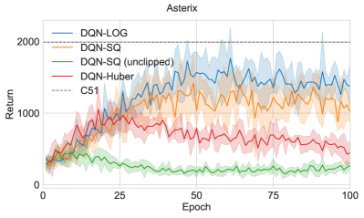
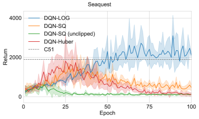
Figure 3: Learning curves on Asterix and Seaquest. The result are averaged over 5 datasets with one standard error. One epoch contains 100k updates.

References

• Abeille et al. (2021) Marc Abeille, Louis Faury, and Clément Calauzènes. Instance-wise minimax-optimal algorithms for logistic bandits. In International Conference on Artificial Intelligence and Statistics (AISTATS), 2021.
• Agarwal et al. (2020) Rishabh Agarwal, Dale Schuurmans, and Mohammad Norouzi. An optimistic perspective on offline reinforcement learning. In International Conference on Machine Learning (ICML), 2020.
• Allen-Zhu et al. (2018) Zeyuan Allen-Zhu, Sébastien Bubeck, and Yuanzhi Li. Make the minority great again: First-order regret bound for contextual bandits. In International Conference on Machine Learning (ICML), 2018.
• Antos et al. (2007) András Antos, Csaba Szepesvári, and Rémi Munos. Fitted Q-iteration in continuous action-space MDPs. In Neural Information Processing Systems (NeurIPS), 2007.
• Antos et al. (2008) András Antos, Csaba Szepesvári, and Rémi Munos. Learning near-optimal policies with Bellman-residual minimization based fitted policy iteration and a single sample path. Machine Learning, 2008.
• Azar et al. (2017) Mohammad Gheshlaghi Azar, Ian Osband, and Rémi Munos. Minimax regret bounds for reinforcement learning. In International Conference on Machine Learning (ICML), 2017.
• Bellemare et al. (2013) Marc G Bellemare, Yavar Naddaf, Joel Veness, and Michael Bowling. The arcade learning environment: An evaluation platform for general agents. Journal of Artificial Intelligence Research, 2013.
• Bellemare et al. (2017) Marc G Bellemare, Will Dabney, and Rémi Munos. A distributional perspective on reinforcement learning. In International Conference on Machine Learning (ICML), 2017.
• Bellemare et al. (2023) Marc G. Bellemare, Will Dabney, and Mark Rowland. Distributional Reinforcement Learning. MIT Press, 2023.
• Bertsekas (1995) D. Bertsekas. Dynamic Programming and Optimal Control. Athena Scientific, 1995.
• Buckman et al. (2021) Jacob Buckman, Carles Gelada, and Marc G Bellemare. The importance of pessimism in fixed-dataset policy optimization. In International Conference on Learning Representations (ICLR), 2021.
• Chen and Jiang (2019) Jinglin Chen and Nan Jiang. Information-theoretic considerations in batch reinforcement learning. In International Conference on Machine Learning (ICML), 2019.
• Dennis and Moré (1974) John E Dennis and Jorge J Moré. A characterization of superlinear convergence and its application to quasi-Newton methods. Mathematics of computation, 1974.
• Ernst et al. (2005) Damien Ernst, Pierre Geurts, and Louis Wehenkel. Tree-based batch mode reinforcement learning. Journal of Machine Learning Research (JMLR), 2005.
• Farahmand (2011) Amir-massoud Farahmand. Regularization in reinforcement learning. PhD thesis, University of Alberta, 2011.
• Foster and Krishnamurthy (2021) Dylan J Foster and Akshay Krishnamurthy. Efficient first-order contextual bandits: prediction, allocation, and triangular discrimination. Neural Information Processing Systems (NeurIPS), 2021.
• Foster et al. (2021) Dylan J Foster, Akshay Krishnamurthy, David Simchi-Levi, and Yunzong Xu. Offline reinforcement learning: fundamental barriers for value function approximation. arXiv preprint arXiv:2111.10919, 2021.
• Freund and Schapire (1997) Yoav Freund and Robert E Schapire. A decision-theoretic generalization of on-line learning and an application to boosting. Journal of computer and system sciences, 1997.
• Janz et al. (2023) David Janz, Shuai Liu, Alex Ayoub, and Csaba Szepesvári. Exploration via linearly perturbed loss minimisation. arXiv preprint arXiv:2311.07565, 2023.
• Jin et al. (2020a) Chi Jin, Akshay Krishnamurthy, Max Simchowitz, and Tiancheng Yu. Reward-free exploration for reinforcement learning. In International Conference on Machine Learning (ICML), 2020a.
• Jin et al. (2020b) Chi Jin, Zhuoran Yang, Zhaoran Wang, and Michael I Jordan. Provably efficient reinforcement learning with linear function approximation. In Conference on Learning Theory (COLT), 2020b.
• Jin et al. (2021) Ying Jin, Zhuoran Yang, and Zhaoran Wang. Is pessimism provably efficient for offline rl? In International Conference on Machine Learning (ICML), 2021.
• Kakade and Langford (2002) Sham Kakade and John Langford. Approximately optimal approximate reinforcement learning. In International Conference on Machine Learning (ICML), 2002.
• Kakade et al. (2020) Sham Kakade, Akshay Krishnamurthy, Kendall Lowrey, Motoya Ohnishi, and Wen Sun. Information theoretic regret bounds for online nonlinear control. Neural Information Processing Systems (NeurIPS), 2020.
• Konidaris et al. (2011) George Konidaris, Sarah Osentoski, and Philip Thomas. Value function approximation in reinforcement learning using the Fourier basis. In AAAI Conference on Artificial Intelligence (AAAI), 2011.
• Lazaric et al. (2012) Alessandro Lazaric, Mohammad Ghavamzadeh, and Rémi Munos. Finite-sample analysis of least-squares policy iteration. Journal of Machine Learning Research (JMLR), 2012.
• Lee et al. (2020) Chung-Wei Lee, Haipeng Luo, Chen-Yu Wei, and Mengxiao Zhang. Bias no more: high-probability data-dependent regret bounds for adversarial bandits and Mdps. Neural Information Processing Systems (NeurIPS), 2020.
• Littman (1996) Michael Lederman Littman. Algorithms for sequential decision-making. PhD thesis, Brown University, 1996.
• Lykouris et al. (2022) Thodoris Lykouris, Karthik Sridharan, and Éva Tardos. Small-loss bounds for online learning with partial information. Mathematics of Operations Research, 2022.
• Machado et al. (2018) Marlos C Machado, Marc G Bellemare, Erik Talvitie, Joel Veness, Matthew Hausknecht, and Michael Bowling. Revisiting the arcade learning environment: Evaluation protocols and open problems for general agents. Journal of Artificial Intelligence Research (JAIR), 2018.
• Mnih et al. (2015) Volodymyr Mnih, Koray Kavukcuoglu, David Silver, Andrei A. Rusu, Joel Veness, Marc G. Bellemare, Alex Graves, Martin Riedmiller, Andreas K. Fidjeland, Georg Ostrovski, Stig Petersen, Charles Beattie, Amir Sadik, Ioannis Antonoglou, Helen King, Dharshan Kumaran, Daan Wierstra, Shane Legg, and Demis Hassabis. Human-level control through deep reinforcement learning. Nature, 2015.
• Moore (1990) Andrew William Moore. Efficient memory-based learning for robot control. Technical report, University of Cambridge, 1990.
• Munos (2003) Rémi Munos. Error bounds for approximate policy iteration. In International Conference on Machine Learning (ICML), 2003.
• Munos and Szepesvári (2008) Rémi Munos and Csaba Szepesvári. Finite-time bounds for fitted value iteration. Journal of Machine Learning Research (JMLR), 2008.
• Neu (2015) Gergely Neu. First-order regret bounds for combinatorial semi-bandits. In Conference on Learning Theory (COLT), 2015.
• Olkhovskaya et al. (2023) Julia Olkhovskaya, Jack Mayo, Tim van Erven, Gergely Neu, and Chen-Yu Wei. First- and second-order bounds for adversarial linear contextual bandits. In Neural Information Processing Systems (NeurIPS), 2023.
• Pires and Szepesvári (2012) Bernardo Ávila Pires and Csaba Szepesvári. Statistical linear estimation with penalized estimators: an application to reinforcement learning. In International Conference on Machine Learning (ICML), 2012.
• Riedmiller (2005) Martin Riedmiller. Neural fitted Q iteration–first experiences with a data efficient neural reinforcement learning method. In European Conference on Machine Learning (ECML), 2005.
• Sutton and Barto (2018) Richard S Sutton and Andrew G Barto. Reinforcement learning: an introduction. MIT press, 2018.
• Topsoe (2000) F. Topsoe. Some inequalities for information divergence and related measures of discrimination. IEEE Transactions on Information Theory, 2000.
• Wagenmaker et al. (2022) Andrew J Wagenmaker, Yifang Chen, Max Simchowitz, Simon Du, and Kevin Jamieson. First-order regret in reinforcement learning with linear function approximation: A robust estimation approach. In International Conference on Machine Learning (ICML), 2022.
• Wang et al. (2023) Kaiwen Wang, Kevin Zhou, Runzhe Wu, Nathan Kallus, and Wen Sun. The benefits of being distributional: small-loss bounds for reinforcement learning. In Advances in Neural Information Processing Systems (NeurIPS), 2023.
• Wang et al. (2024) Kaiwen Wang, Owen Oertell, Alekh Agarwal, Nathan Kallus, and Wen Sun. More benefits of being distributional: Second-order bounds for reinforcement learning. arXiv preprint arXiv:2402.07198, 2024.
• Xie and Jiang (2021) Tengyang Xie and Nan Jiang. Batch value-function approximation with only realizability. In International Conference on Machine Learning (ICML), 2021.
• Yang and Wang (2019) Lin Yang and Mengdi Wang. Sample-optimal parametric Q-learning using linearly additive features. In International Conference on Machine Learning (ICML), 2019.
• Zhang (2023) Tong Zhang. Mathematical Analysis of Machine Learning Algorithms. Cambridge University Press, 2023.