Multiple correlations of spectra
for higher rank Anosov representations

Abstract.

We describe multiple correlations of Jordan and Cartan spectra for any finite number of Anosov representations of a finitely generated group. This extends our previous work on correlations of length and displacement spectra for rank one convex cocompact representations. Examples include correlations of the Hilbert length spectra for convex projective structures on a closed surface as well as correlations of eigenvalue gaps and singular value gaps for Hitchin representations. We relate the correlation problem to the counting problem for Jordan and Cartan projections of an Anosov subgroup with respect to a family of carefully chosen truncated hypertubes, rather than in tubes as in our previous work. Hypertubes go to infinity in a linear subspace of directions, while tubes go to infinity in a single direction and this feature presents a novel difficulty in this higher rank correlation problem.

1. Introduction

In this paper, we describe multiple correlations of Jordan and Cartan spectra for any finite number of Anosov representations of a finitely generated group into semisimple real algebraic groups.

We begin by discussing special cases of our result for different classes of geometric structures on a closed surface. Let $S$ be a closed orientable surface of genus $g\geq 2$. Let $\rho$ be a discrete faithful representation of the fundamental group $\Sigma=\pi_{1}(S)$ into $\operatorname{PSL}_{2}\mathbb{R}$, which can be viewed as an element of the Teichmüller space $\cal{T}(S)\simeq\mathbb{R}^{6g-6}$ after identifying conjugate representations. Hence $\rho$ induces a hyperbolic structure $S_{\rho}\simeq\rho(\Sigma)\backslash\mathbb{H}^{2}$ and a length function $\ell_{\rho}$ which assigns to the conjugacy class $[\sigma]\in[\Sigma]$ the hyperbolic length of the corresponding closed geodesic in $S_{\rho}$. The prime geodesic theorem due to Huber [18] gives an asymptotic for the number of closed geodesics in $S_{\rho}$ of hyperbolic length at most $T$:

$$\#\{[\sigma]\in[\Sigma]:\ell_{\rho}(\sigma)\leq T\}\sim\frac{e^{T}}{T}\quad\text{as }T\to\infty.$$

Given a $d$-tuple $\boldsymbol{\rho}=(\rho_{1},\dots,\rho_{d})$ of distinct elements in $\cal{T}(S)$, it is natural to ask how the length functions $\ell_{\rho_{1}},\dots,\ell_{\rho_{d}}$ are correlated. In [5], we proved that for any interior vector $\boldsymbol{r}=(r_{1},\dots,r_{d})$ in the smallest closed cone containing all vectors $(\ell_{\rho_{1}}(\sigma),\dots,\ell_{\rho_{d}}(\sigma))$ for $\sigma\in\Sigma$, there exists $\delta=\delta(\boldsymbol{\rho},\boldsymbol{r})>0$ such that for any $\varepsilon_{1},\dots,\varepsilon_{d}>0$, we have as $T\to\infty$,

$$\#\{[\sigma]\in[\Sigma]:r_{i}T\leq\ell_{\rho_{i}}(\sigma)\leq r_{i}T+\varepsilon_{i}\text{ for all $1\leq i\leq d$}\}\sim c\cdot\frac{e^{\delta T}}{T^{(d+1)/2}}$$

for some $c>0$. This was earlier proved by Schwarz-Sharp [31] for $d=2$ and $\boldsymbol{r}=(1,1)$ (see [12] for $d=2$ and a general $\boldsymbol{r}$). Indeed, we obtained an analogous result on correlations of length spectra for any finite number of rank one convex cocompact representations of a finitely generated group [5].

Hilbert length spectra for convex projective structures

Another space of interesting geometric structures on a closed surface $S$ is the space $\cal{C}(S)$ of convex projective structures. A discrete faithful representation $\rho:\Sigma\to\operatorname{PGL}_{3}\mathbb{R}$ is called convex projective if its image acts cocompactly on some properly convex domain $\Omega\subset\mathbb{R}\mathbb{P}^{2}$. Such a representation $\rho$ endows a convex projective structure on $S$ which we denote by $S_{\rho}\simeq\rho(\Gamma)\backslash\Omega$. The space $\cal{C}(S)$ can be identified with the space of convex projective representations $\rho:\Sigma\to\operatorname{PGL}_{3}\mathbb{R}$ modulo conjugation. Goldman showed that $\cal{C}(S)$ is homeomorphic to $\mathbb{R}^{16g-16}$ and contains the Teichmüller space $\cal{T}(S)$ as a $(6g-6)$-dimensional subspace [13]. For $\rho\in{\cal C}(S)$ and a conjugacy class $[\sigma]\in[\Sigma]$, denote by $\ell^{\operatorname{H}}_{\rho}(\sigma)$ the Hilbert length of the corresponding closed geodesic (cf. (6.3)). Benoist proved the prime geodesic theorem for $S_{\rho}$:

(1.1) $$\#\{[\sigma]\in[\Sigma]:\ell^{\operatorname{H}}_{\rho}(\sigma)\leq T\}\sim\frac{e^{\delta_{\rho}T}}{\delta_{\rho}T}\quad\text{as }T\to\infty,$$

where $\delta_{\rho}$ is the topological entropy of the Hilbert geodesic flow on $S_{\rho}$ [1].

Blayac-Zhu showed that (1.1) holds more generally for strongly convex cocompact projective representations [3]. Let $\Gamma$ be a finitely generated group. Following [8, Definition 1.1], a discrete faithful representation $\rho:\Gamma\to\operatorname{PGL}_{3}\mathbb{R}$ is strongly convex cocompact if $\rho(\Gamma)$ acts on some strictly convex domain $\Omega$, and the action is cocompact on the convex hull of its limit set. For any $d$-tuple $\boldsymbol{\rho}=(\rho_{1},\dots,\rho_{d}):\Gamma\to\operatorname{PGL}_{3}\mathbb{R}$ of Zariski dense strongly convex cocompact projective representations, let $\cal{L}_{\boldsymbol{\rho}}\subset\mathbb{R}^{d}$ denote the smallest closed cone containing all vectors $(\ell^{\operatorname{H}}_{\rho_{1}}(\gamma),\dots,\ell^{\operatorname{H}}_{\rho_{d}}(\gamma))$ for $\gamma\in\Gamma$. If $\boldsymbol{\rho}$ is independent, i.e., for all $i\neq j$, $\rho_{i}$ is not conjugate to neither $\rho_{j}$ nor the contragradient $\rho_{j}^{*}$, then $\cal{L}_{\boldsymbol{\rho}}$ has non-empty interior. The following is a special case of our main theorem:

Theorem 1.1 (Multiple correlations of Hilbert length spectra).

Let $d\geq 2$ and $\boldsymbol{\rho}=(\rho_{1},\dots,\rho_{d}):\Gamma\to\operatorname{PGL}_{3}(\mathbb{R})$ be an independent $d$-tuple of Zariski dense strongly convex cocompact projective representations. Then for any interior vector $\boldsymbol{r}=(r_{1},\dots,r_{d})\in\cal{L}_{\boldsymbol{\rho}}$, there exists $\delta=\delta_{\boldsymbol{\rho}}(\boldsymbol{r})>0$ such that for any $\varepsilon_{1},\dots,\varepsilon_{d}>0$, we have as $T\to\infty$,

$$\#\{[\sigma]\in[\Gamma]:r_{i}T\leq\ell^{\operatorname{H}}_{\rho_{i}}(\sigma)\leq r_{i}T+\varepsilon_{i}\text{ for all }1\leq i\leq d\}\sim c\cdot\frac{e^{\delta T}}{T^{(d+1)/2}}$$

for some $c>0$. Moreover, we have the upper bound:

$$\delta_{\boldsymbol{\rho}}(\boldsymbol{r})\leq\min_{1\leq i\leq d}\delta_{\rho_{i}}r_{i},$$

which is strict when all $\delta_{\rho_{i}}r_{i}$ are equal.

Remark 1.2.

Using the thermodynamic approach of Schwartz-Sharp [31], Dai-Martone [7] proved Theorem 1.1 for $d=2$ and $\boldsymbol{r}=(1/\delta_{\rho_{1}},1/\delta_{\rho_{2}})$.

Eigenvalue and singular value gaps for Hitchin representations

For $n\geq 2$, the Hitchin component $\cal{H}_{n}$ of $\operatorname{Hom}(\Sigma,\operatorname{PSL}_{n}\mathbb{R})$ is the connected component containing the representation $\tau_{n}\circ\rho_{0}:\Sigma\to\operatorname{PSL}_{n}\mathbb{R}$ where $\rho_{0}:\Sigma\to\operatorname{PSL}_{2}\mathbb{R}$ is a discrete and faithful representation and $\tau_{n}:\operatorname{PSL}_{2}\mathbb{R}\to\operatorname{PSL}_{n}\mathbb{R}$ is the irreducible representation which is unique up to conjugation [17]. Let $\rho\in\cal H_{n}$ be a Hitchin representation. Labourie [22] proved that for all nontrivial $\sigma\in\Sigma$, $\rho(\sigma)$ has all distinct positive eigenvalues. We denote their logarithms in the decreasing order by

(1.2) $$\lambda(\rho(\sigma))=(\lambda_{1}(\rho(\sigma)),\dots,\lambda_{n}(\rho(\sigma)))\in\mathbb{R}^{n}.$$

We denote the logarithms of the singular values of $\rho(\sigma)$ in the decreasing order by

(1.3) $$\mu(\rho(\sigma))=(\mu_{1}(\rho(\sigma)),\dots,\mu_{n}(\rho(\sigma)))\in\mathbb{R}^{n}.$$

For $1\leq k\leq n-1$, consider the linear form $\alpha_{k}:\mathbb{R}^{n}\to\mathbb{R}$ given by

$$\alpha_{k}(x_{1},\dots,x_{n})=x_{k}-x_{k+1}.$$

Sambarino [29] proved that for any Zariski dense $\rho\in\cal{H}_{n}$ and $1\leq k\leq n-1$:

(1.4) $$\#\{[\sigma]\in[\Sigma]:\alpha_{k}(\lambda(\rho(\sigma)))\leq T\}\sim\frac{e^{\delta_{k}T}}{\delta_{k}T}\quad\text{as }T\to\infty.$$

where $\delta_{k}=\lim_{T\to\infty}\frac{1}{T}\log\#\{[\sigma]\in[\Sigma]:\alpha_{k}(\lambda(\rho(\sigma))\leq T\}.$ Moreover, Potrie-Sambarino [25, Theorem B] proved that $\delta_{k}=1$.

For a $d$-tuple $\boldsymbol{\rho}=(\rho_{1},\dots,\rho_{d})$ of Zariski dense Hitchin representations in $\cal{H}_{n}$ and $\boldsymbol{\beta}=(\beta_{1},\dots,\beta_{d})\in\Pi^{d}$, where $\Pi=\{\alpha_{1},\dots,\alpha_{d}\}$, denote by $\cal{L}_{\boldsymbol{\beta}}=\cal{L}_{\boldsymbol{\rho},\boldsymbol{\beta}}\subset\mathbb{R}^{d}$ the smallest closed cone containing all vectors

$$(\beta_{1}(\lambda(\rho_{1}(\sigma))),\dots,\beta_{d}(\lambda(\rho_{d}(\sigma))))\text{ for }\sigma\in\Sigma.$$

For example, all $\beta_{i}$, $1\leq i\leq d$, can be $\alpha_{1}$. If $\boldsymbol{\rho}$ is independent, in the sense that for all $i\neq j$, $\rho_{i}$ is not conjugate to neither $\rho_{j}$ nor the contragradient $\rho_{j}^{*}$, then $\cal{L}_{\boldsymbol{\beta}}$ has non-empty interior. We prove the following:

Theorem 1.3 (Multiple correlations of eigenvalue and singular value gaps).

Let $d\geq 2$ and $\boldsymbol{\rho}=(\rho_{1},\dots,\rho_{d}):\Sigma\to\operatorname{PSL}_{n}(\mathbb{R})$ be a $d$-tuple of independent Zariski dense Hitchin representations. Let $\boldsymbol{\beta}=(\beta_{1},\dots,\beta_{d})\in\Pi^{d}$. Then for any interior vector $\boldsymbol{r}=(r_{1},\dots,r_{d})\in\cal{L}_{\boldsymbol{\beta}}$, there exists $\delta=\delta_{\boldsymbol{\rho},\boldsymbol{\beta}}(\boldsymbol{r})>0$ such that for any $\varepsilon_{1},\dots,\varepsilon_{d}>0$, we have as $T\to\infty$,

$$\#\{[\sigma]\in[\Sigma]:r_{i}T\leq\beta_{i}(\lambda(\rho_{i}(\sigma)))\leq r_{i}T+\varepsilon_{i}\text{ for all }1\leq i\leq d\}\sim c\cdot\frac{e^{\delta T}}{T^{(d+1)/2}}$$

and

$$\#\{\sigma\in\Sigma:r_{i}T\leq\beta_{i}(\mu(\rho_{i}(\sigma)))\leq r_{i}T+\varepsilon_{i}\text{ for all }1\leq i\leq d\}\sim c^{\prime}\cdot c\cdot\frac{e^{\delta T}}{T^{(d-1)/2}}$$

where $c=c(\boldsymbol{\rho},\boldsymbol{\beta},\boldsymbol{r},\varepsilon_{1},\dots,\varepsilon_{d})>0$ and $c^{\prime}=c^{\prime}(\boldsymbol{\rho},\boldsymbol{\beta,\boldsymbol{r}})>0$. Moreover, we have the upper bound

(1.5) $$\delta_{\boldsymbol{\rho},\boldsymbol{\beta}}(\boldsymbol{r})\leq\min_{1\leq i\leq d}r_{i}$$

and if all $r_{i}$ are equal, then the inequality is strict.

We note that the upper bound (1.5) is independent of $\boldsymbol{\rho}$ and $\boldsymbol{\beta}$; the reason behind this is the aforementioned fact that $\delta_{k}=1$ in (1.4) for all Hitchin representations [25, Theorem B].

Remark 1.4.

When $d=2$, $\beta_{1}=\beta_{2}$ and $\boldsymbol{r}=(1,1)$, the eigenvalue gap statement was proved by Dai-Martone [7].

Multiple correlations of Jordan and Cartan spectra

The aforementioned examples are all Anosov representations ([11], [22]). The main results of this paper are multiple correlations of Jordan and Cartan spectra for general Zariski dense Anosov representations. Let $G$ be a connected semisimple real algebraic group and fix a Cartan decomposition $G=K(\exp\mathfrak{a}^{+})K$ where $K$ is a maximal compact subgroup, $A$ is a maximal real split torus and $\mathfrak{a}^{+}$ is a positive Weyl chamber of $\mathfrak{a}=\operatorname{Lie}A$. Let $\mu:G\to\mathfrak{a}^{+}$ denote the Cartan projection map, that is, $\mu(g)$ is the unique element of $\mathfrak{a}^{+}$ such that $g\in K(\exp\mu(g))K$ for all $g\in G$. Let $M$ denote the centralizer of $A$ in $K$.

A finitely generated subgroup $\Gamma<G$ is called Anosov if there exists $C>0$ such that for every simple root $\alpha$ of $(\mathfrak{g},\mathfrak{a})$ and $\gamma\in\Gamma$, we have

(1.6) $$\alpha(\mu(\gamma))\geq C|\gamma|-C^{-1}$$

where $|\cdot|$ denotes the word length of $\Gamma$ with respect to a fixed finite set of generators. This definition is due to Kapovich-Leeb-Porti [19] (see also [22], [15], [14] for other equivalent definitions). Every nontrivial element $\gamma\in\Gamma$ is loxodromic [15, Lemma 3.1] and hence conjugate to an element $\exp(\lambda(\gamma))m(\gamma)$ where $\lambda(\gamma)\in\operatorname{int}\mathfrak{a}^{+}$ is the Jordan projection of $\gamma$ and $m(\gamma)\in M$. The conjugacy class $[m(\gamma)]\in[M]$ is uniquely determined and called the holonomy of $\gamma$. We note that $\lambda(\gamma)$ and $[m(\gamma)]$ depend only on the conjugacy class of $\gamma$. The limit cone $\cal L_{\Gamma}\subset\mathfrak{a}^{+}$ of $\Gamma$ is the smallest closed cone containing $\lambda(\Gamma)$; this is a convex cone with non-empty interior when $\Gamma$ is Zariski dense in $G$ [2].

For a Zariski dense Anosov subgroup $\Gamma<G$, Sambarino [29] proved that for any $\varphi\in\mathfrak{a}^{*}$ which is positive on $\cal{L}_{\Gamma}-\{0\}$,

(1.7) $$\#\{[\gamma]\in[\Gamma]:\varphi(\lambda(\gamma))\leq T\}\sim\frac{e^{\delta_{\varphi}T}}{\delta_{\varphi}T}\quad\text{as }T\to\infty$$

where $\delta_{\varphi}=\delta_{\Gamma,\varphi}=\lim_{T\to\infty}\frac{1}{T}\log\#\{[\gamma]\in[\Gamma]:\varphi(\lambda(\gamma))\leq T\}.$ See also [4, Corollaries 1.4 and 1.10] for a different proof which also includes holonomies.

In order to state our correlation theorems, let $G_{1},\dots,G_{d}$ be any connected semisimple real algebraic groups for $d\geq 2$. Fix a finitely generated group $\Sigma$ and let

$$\boldsymbol{\rho}=(\rho_{i}:\Sigma\to G_{i})_{1\leq i\leq d}$$

be a $d$-tuple of Anosov representations. We assume that $\boldsymbol{\rho}(\Sigma)$ is Zariski dense in $\prod_{i=1}^{d}G_{i}$. We use the same notations for $G_{i}$ as we did for $G$ but with a subscript $i$. Let

$$\boldsymbol{\varphi}:\bigoplus_{i=1}^{d}\mathfrak{a}_{i}\to\mathbb{R}^{d}$$

be a linear map given by $\boldsymbol{\varphi}=(\varphi_{i}:\mathfrak{a}_{i}\to\mathbb{R})_{1\leq i\leq d}$ where $\varphi_{i}$ is a linear form on $\mathfrak{a}_{i}$ which is positive on $\cal{L}_{\rho_{i}(\Sigma)}-\{0\}$ for each $i$. Let $\cal{L}_{\boldsymbol{\varphi}}=\cal{L}_{\boldsymbol{\rho},\boldsymbol{\varphi}}\subset\mathbb{R}^{d}$ be the smallest closed cone containing all vectors

$$\boldsymbol{\varphi}(\lambda(\boldsymbol{\rho}(\sigma)))=(\varphi_{1}(\lambda(\rho_{1}(\sigma))),\dots,(\varphi_{d}(\lambda(\rho_{d}(\sigma)))\text{ for }\sigma\in\Sigma.$$

We define the holonomy group $M_{\boldsymbol{\rho}}$ of $\boldsymbol{\rho}$ as the smallest closed subgroup of $\prod_{i=1}^{d}M_{i}$ generated by all the $d$-tuples of holonomies

$${m}(\boldsymbol{\rho}(\sigma))=(m(\rho_{1}(\sigma)),\dots,m(\rho_{d}(\sigma))\text{ for }\sigma\in\Sigma.$$

By [16, Corollary 1.10], this is a finite index normal subgroup of $\prod_{i=1}^{d}M_{i}$. Let $\operatorname{Vol}_{M_{\boldsymbol{\rho}}}$ denote the Haar probability measure on $M_{\boldsymbol{\rho}}$.

The following is the main theorem of this paper:

Theorem 1.5 (Multiple correlations of Jordan and Cartan spectra).

For any interior vector $\boldsymbol{r}=(r_{1},\dots,r_{d})\in\cal{L}_{\boldsymbol{\varphi}}$, there exists $\delta=\delta_{\boldsymbol{\rho},\boldsymbol{\varphi}}(\boldsymbol{r})>0$ such that for any $\varepsilon_{1},\dots,\varepsilon_{d}>0$ and for any conjugation invariant Borel subset $\Theta<M_{\boldsymbol{\rho}}$ with $\operatorname{Vol}_{M_{\boldsymbol{\rho}}}(\partial\Theta)=0$, we have as $T\to\infty$,

$$\#\{[\sigma]\in[\Sigma]:\,\boldsymbol{\varphi}(\lambda(\boldsymbol{\rho}(\sigma)))\in\prod_{i=1}^{d}[r_{i}T,r_{i}T+\varepsilon_{i}],\,m(\boldsymbol{\rho}(\sigma))\in\Theta\}\\ \sim c\cdot\frac{e^{\delta T}}{T^{(d+1)/2}}\operatorname{Vol}_{M_{\boldsymbol{\rho}}}(\Theta)$$

and

$$\#\{\sigma\in\Sigma:\boldsymbol{\varphi}(\mu(\boldsymbol{\rho}(\sigma)))\in\prod_{i=1}^{d}[r_{i}T,r_{i}T+\varepsilon_{i}]\}\sim c^{\prime}\cdot c\cdot\frac{e^{\delta T}}{T^{(d-1)/2}}$$

where $c=c(\boldsymbol{\rho},\boldsymbol{\varphi},\boldsymbol{r},\varepsilon_{1},\dots,\varepsilon_{d})>0$ and $c^{\prime}=c^{\prime}(\boldsymbol{\rho},\boldsymbol{\varphi},\boldsymbol{r})>0$. Moreover, we have the upper bound

(1.8) $$\delta_{\boldsymbol{\rho},\boldsymbol{\varphi}}(\boldsymbol{r})\leq\min_{1\leq i\leq d}\delta_{\rho_{i}(\Sigma),\varphi_{i}}r_{i}$$

which is strict when all $\delta_{\rho_{i}(\Sigma),\varphi_{i}}r_{i}$ are equal.

Remark 1.6.

The exponent $\delta=\delta_{\boldsymbol{\rho},\boldsymbol{\varphi}}(\boldsymbol{r})$ is given by $\psi_{\boldsymbol{\rho}(\Sigma)}(\mathsf{v}^{\star})$ where $\psi_{\boldsymbol{\rho}(\Sigma)}$ is the growth indicator of the subgroup $\boldsymbol{\rho}(\Sigma)<\prod_{i=1}^{d}G_{i}$ and $\mathsf{v}^{\star}=\mathsf{v}^{\star}(\boldsymbol{\varphi},\boldsymbol{r})$ is the unique $(\boldsymbol{\varphi},\boldsymbol{r})$-critical vector (see Theorem 6.1 and the proof of Theorem 1.5). The bound (1.8) is then deduced from [20] from which it also follows that the equality in (1.8) happens for exactly $d$-number of directions.

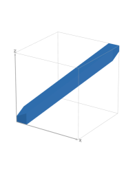
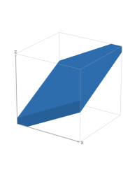
Figure 1. Tube vs. hypertube.

Comparison with the previous work

We have previously proved Theorem 1.5 in the case where every $G_{i}$ has rank one [5] (under a slightly stronger assumption on $\boldsymbol{\varphi}$). There is a main conceptual difference between that case and the current general case we are dealing with. In that setting, the rank of the product $\prod_{i=1}^{d}G_{i}$ is equal to $d$ and hence the map $\boldsymbol{\varphi}:\bigoplus_{i=1}^{d}\mathfrak{a}_{i}\simeq\mathbb{R}^{d}\to\mathbb{R}^{d}$ is an isomorphism. Therefore the set $\boldsymbol{\varphi}^{-1}(\prod_{i=1}^{d}[r_{i}T,r_{i}T+\varepsilon_{i}])=\boldsymbol{\varphi}^{-1}(\prod_{i=1}^{d}[0,\varepsilon_{i}])+T\boldsymbol{\varphi}^{-1}(\boldsymbol{r})$ is a translation of a compact subset and sweeps out a tube going to infinity along the direction of a vector $\boldsymbol{\varphi}^{-1}(\boldsymbol{r})$ as $T$ increases. Note that there is only one direction of a tube which tends to infinity and hence only one way to truncate the tubes for studying asymptotics.

However, when some $G_{i}$ has rank at least 2, the linear map

$$\boldsymbol{\varphi}:\bigoplus_{i=1}^{d}\mathfrak{a}_{i}\simeq\mathbb{R}^{\sum_{i=1}^{d}\operatorname{rank}G_{i}}\to\mathbb{R}^{d}$$

is not injective and hence the preimage $\boldsymbol{\varphi}^{-1}(\boldsymbol{r})$ is an affine subspace of positive dimension. As a result, the union $\bigcup_{T>0}\boldsymbol{\varphi}^{-1}(\prod_{i=1}^{d}[r_{i}T,r_{i}T+\varepsilon_{i}])$ is a hypertube which goes to infinity in all directions of the affine subspace $\boldsymbol{\varphi}^{-1}(\boldsymbol{r})$ (see Fig. 1). This feature presents a novel difficulty in this higher rank correlation problem, since unlike for tubes, there are many different truncations of the hypertube that can be considered. Coming up with a truncation simultaneously adapted to $\boldsymbol{\rho}$ and the linear map $\boldsymbol{\varphi}$ that can be analyzed is the main challenge in the current setting.

Outline of the proof of Theorem 1.5

For simplicity, we will discuss only correlations of Jordan spectra. We first explain the relation between correlations of Jordan spectra for a $d$-tuple $\boldsymbol{\rho}$ of Anosov representations and counting the Jordan spectra of a single Anosov subgroup $\Gamma$.

The hypotheses in Theorem 1.5 imply that $\Gamma=\boldsymbol{\rho}(\Sigma)$ is a Zariski dense Anosov subgroup of the product $G=\prod_{i=1}^{d}G_{i}$, that the cone $\cal{L}_{\boldsymbol{\varphi}}$ coincides with $\boldsymbol{\varphi}(\cal{L}_{\Gamma})$ and that the restriction $\boldsymbol{\varphi}|_{\cal{L}_{\Gamma}}$ is a proper map. We will in fact study a general Zariski dense Anosov subgroup $\Gamma$ of any semisimple real algebraic group $G$ and a general surjective linear map

$$\boldsymbol{\varphi}:\mathfrak{a}\to\mathbb{R}^{d}\;\text{such that }\boldsymbol{\varphi}|_{\cal{L}_{\Gamma}}\text{ is proper}.$$

In particular, $1\leq d\leq\mathrm{rank}(G)=\dim\mathfrak{a}$ and $\ker\boldsymbol{\varphi}$ has dimension $\mathrm{rank}(G)-d$. Fix a vector $\boldsymbol{r}=(r_{1},\dots,r_{d})$ in the interior of the cone $\boldsymbol{\varphi}(\cal{L}_{\Gamma})$ and $\varepsilon_{1},\dots,\varepsilon_{d}>0$. The properness of $\boldsymbol{\varphi}|_{\cal{L}_{\Gamma}}$ implies that for each $T>0$,

(1.9) $$\#\{[\gamma]\in[\Gamma]:\,\boldsymbol{\varphi}(\lambda(\gamma))\in\prod_{i=1}^{d}[r_{i}T,r_{i}T+\varepsilon_{i}]\}<\infty$$

and our goal is to find an asymptotic as $T\to\infty$. Geometrically, for any choice of $\mathsf{v}\in\mathfrak{a}^{+}$ with $\boldsymbol{\varphi}(\mathsf{v})=\boldsymbol{r}$, the shape of the set

$$\{\mathsf{u}\in\mathfrak{a}:\boldsymbol{\varphi}(\mathsf{u})\in\prod_{i=1}^{d}[r_{i}T,r_{i}T+\varepsilon_{i}]\}\cap\cal L_{\Gamma}$$

is an infinite prism which slides in the direction of $\mathsf{v}$ as $T$ increases, intersected with the limit cone $\cal L_{\Gamma}$. We consider their union:

(1.10) $$\mathbb{T}=\bigcup_{T>0}\{\mathsf{u}\in\cal L_{\Gamma}:\boldsymbol{\varphi}(\mathsf{u})\in\prod_{i=1}^{d}[r_{i}T,r_{i}T+\varepsilon_{i}]\}.$$

If $\mathsf{Q}\subset\mathfrak{a}$ is a compact subset such that $\boldsymbol{\varphi}(\mathsf{Q})=\prod_{i=1}^{d}[0,\varepsilon_{i}]$ and $V=\boldsymbol{\varphi}^{-1}(\mathbb{R}\boldsymbol{r})$ is the preimage of the line $\mathbb{R}\boldsymbol{r}$, then we have (Lemma 4.2)

$$\mathbb{T}=(\mathsf{Q}+V)\cap\cal L_{\Gamma};$$

and a set of this form will be called a hypertube as one can think of $\mathbb{T}$ as obtained from translating $\mathsf{Q}$ in all directions of $V\cap\cal L_{\Gamma}$ (see Fig. 2).

Figure 2. A hypertube of $\cal{L}$.

For each $T>0$, consider a truncation $\mathbb{T}_{T}:$

$$\mathbb{T}_{T}:=\{\mathsf{u}\in\cal L_{\Gamma}:\boldsymbol{\varphi}(\mathsf{u})\in\prod_{i=1}^{d}[0,r_{i}T+\varepsilon_{i}]\}.$$

We show that for some vector $\mathsf{v}^{\star}\in\mathfrak{a}^{+}$,

(1.11) $$\#\{[\gamma]\in[\Gamma]:\lambda(\gamma)\in\mathbb{T}_{T}\}\sim c\cdot\frac{e^{\psi_{\Gamma}(\mathsf{v}^{\star})T}}{T^{(d+1)/2}}\quad\text{as $T\to\infty$}$$

where $\psi_{\Gamma}$ is the growth indicator of $\Gamma$ (see (2.1)) and $c>0$ is a constant (Theorem 5.10). A priori, the existence of $\mathsf{v}^{\star}\in\mathfrak{a}^{+}$ satisfying (1.11) is not clear at all. To explain where to find such a vector $\mathsf{v}^{\star}\in\mathfrak{a}^{+}$, observe that for any vector $\mathsf{v}\in\mathfrak{a}^{+}\cap\boldsymbol{\varphi}^{-1}(\boldsymbol{r})$, the truncation $\mathbb{T}_{T}$ can be expressed as

$$\mathbb{T}_{T}=(\mathsf{Q}+[0,T]\mathsf{v}+\ker\boldsymbol{\varphi})\cap\cal L_{\Gamma}.$$

When $\mathbb{T}$ is a tube, such a vector $\mathsf{v}$ is uniquely determined, and this $\mathsf{v}$ is $\mathsf{v}^{\star}$, satisfying (1.11). In a general hypertube case, there is a positive dimensional choice of such $\mathsf{v}\in\boldsymbol{\varphi}^{-1}(\boldsymbol{r})$. Using the Anosov property of $\Gamma$, we show that there exists a unique vector $\mathsf{v}^{\star}\in\operatorname{int}\cal{L}\cap\boldsymbol{\varphi}^{-1}(\boldsymbol{r})$ such that

$$\ker\boldsymbol{\varphi}=V\cap\ker\psi_{\mathsf{v}^{\star}},$$

where $\psi_{\mathsf{v}^{\star}}\in\mathfrak{a}^{*}$ is the unique linear form tangent to $\psi_{\Gamma}$ at ${\mathsf{v}^{\star}}$ (Proposition 3.4). We call $\mathsf{v}^{\star}$ a $(\boldsymbol{\varphi},\boldsymbol{r})$-critical vector. Moreover $\mathsf{v}^{\star}$ satisfies (Lemma 3.6):

$$\psi_{\Gamma}(\mathsf{v}^{\star})=\sup_{\mathsf{w}\in\operatorname{int}\cal{L},\,\boldsymbol{\varphi}(\mathsf{w})=\boldsymbol{r}}\psi_{\Gamma}(\mathsf{w}).$$

Once we express the truncation $\mathbb{T}_{T}$ as

$$\mathbb{T}_{T}=(\mathsf{Q}+[0,T]\mathsf{v}^{\star}+(V\cap\ker\psi_{\mathsf{v}^{\star}}))\cap\cal L_{\Gamma}$$

using the critical vector $\mathsf{v}^{\star}$, we can use the framework of our previous work [5] to prove (1.11) using local mixing Theorem 5.3.

The reason why a formula like (1.11) is relevant to (1.9) is because we can find continuous functions $b_{1},b_{2}\in C(\mathsf{Q})$ such that for all $T>0$,

$$\{\mathsf{u}\in\cal L_{\Gamma}:\boldsymbol{\varphi}(\mathsf{u})\in\prod_{i=1}^{d}[r_{i}T,r_{i}T+\varepsilon_{i}]\}=\mathbb{T}_{T,b_{1}}(\mathsf{v}^{\star})-\mathbb{T}_{T,b_{2}}(\mathsf{v}^{\star})$$

where

$$\mathbb{T}_{T,b_{i}}(\mathsf{v}^{\star})=\{\mathsf{q}+\mathsf{v}^{\prime}+t\mathsf{v}^{\star}\in\mathbb{T}\cap\cal L_{\Gamma}:\mathsf{q}\in\mathsf{Q},\,\mathsf{v}^{\prime}\in V\cap\ker\psi_{\mathsf{v}^{\star}},\,0\leq t\leq T+b_{i}({\mathsf{q}})\}.$$

Indeed, we show (1.11) for $\mathbb{T}_{T,b_{i}}(\mathsf{v}^{\star})$ in place of $\mathbb{T}_{T}$ and deduce the asymptotic for (1.9).

Organization

• In Section 2, we recall some preliminaries on Lie theory and discrete subgroups.

• In Section 3, we specialize to Zariski dense Anosov subgroups $\Gamma<G$ and study linear maps $\boldsymbol{\varphi}:\mathfrak{a}\to\mathbb{R}^{d}$ which are proper on $\cal{L}_{\Gamma}$. We prove the existence and uniqueness of a $(\boldsymbol{\varphi},\boldsymbol{r})$-critical direction of $\Gamma$ for any $\boldsymbol{r}\in\operatorname{int}\boldsymbol{\varphi}(\cal{L}_{\Gamma})$ (Proposition 3.4).

• In Section 4, we define hypertubes (Definition 4.1) and their truncations. We explain the relationship between correlations of linearized Jordan and Cartan spectra for Anosov representations and counting Jordan and Cartan projections in hypertubes of an Anosov subgroup.

• In Section 5, we prove joint equidistribution of Jordan projections in hypertubes and holonomies of $\Gamma$ (Theorem 5.2) and equidistribution of $\Gamma$ in bisectors defined using hypertubes (Theorem 5.11), generalizing [5]. The asymptotics for counting Jordan and Cartan projections in hypertubes of are deduced from these equidistribution results (Theorems 5.10 and 5.11).

• In Section 6, we use the results of the previous sections to deduce Theorem 6.1 on asymptotics for linearly correlated Jordan and Cartan projections of $\Gamma$. The correlation theorems in the introduction are then deduced from Theorem 6.1.

2. Preliminaries on discrete subgroups of $G$

Throughout the paper, let $G$ be a connected semisimple real algebraic group. Fixing a Cartan involution of the Lie algebra $\mathfrak{g}$ of $G$, let $\mathfrak{g}=\mathfrak{k}\oplus\mathfrak{p}$ be the eigenspace decomposition corresponding to the eigenvalues $+1$ and $-1$ respectively. Let $K<G$ be the maximal compact subgroup whose Lie algebra is $\mathfrak{k}$. Let $\mathfrak{a}\subset\mathfrak{p}$ be a maximal abelian subalgebra and choose a closed positive Weyl chamber $\mathfrak{a}^{+}\subset\mathfrak{a}$. We denote by $\Phi^{+}$ the set of all positive roots for $(\mathfrak{g},\mathfrak{a})$ with respect to the choice of $\mathfrak{a}^{+}$. Let $w_{0}\in K$ be a representative of the element in the Weyl group such that $\operatorname{Ad}_{w_{0}}(\mathfrak{a}^{+})=-\mathfrak{a}^{+}$. The map $\mathsf{i}:\mathfrak{a}^{+}\to\mathfrak{a}^{+}$ defined by $\mathsf{i}(\mathsf{w})=-\operatorname{Ad}_{w_{0}}(\mathsf{w})$ is called the opposition involution of $G$. Let $A=\exp\mathfrak{a}$ and $A^{+}=\exp\mathfrak{a}^{+}$.

Let $P$ be the minimal parabolic subgroup of $G$ given as $P=MAN$ where $M$ is the centralizer of $A$ in $K$ and $\log N$ consists of all root subspaces corresponding to positive roots. The quotient $\cal{F}:=G/P$ is called the Furstenberg boundary of $G$. By the Iwasawa decomposition $G=KAN$, we have $G/P\simeq K/M$. The Iwasawa cocycle $\sigma:G\times\cal{F}\to\mathfrak{a}$ is the map which assigns to each $(g,kM)\in G\times\cal{F}$ the unique element $\sigma(g,kM)\in\mathfrak{a}$ such that $gk\in K\exp(\sigma(g,\xi))N$. The $\mathfrak{a}$-valued Busemann function $\beta:\cal{F}\times G\times G\to\mathfrak{a}$ is defined by

$$\beta_{\xi}(g_{1},g_{2})=\sigma(g_{1}^{-1},\xi)-\sigma(g_{2}^{-1},\xi)$$

for all $g_{1},g_{2}\in G$ and $\xi\in\cal{F}$.

Cartan and Jordan projections

For $g\in G$, let $\mu(g)$ denote the Cartan projection of $g$, i.e., $\mu(g)\in\mathfrak{a}^{+}$ is the unique element in $\mathfrak{a}^{+}$ such that $g\in K\exp(\mu(g))K.$ Any non-trivial element $g\in G$ can be written as the commuting product $g=g_{h}g_{e}g_{u}$ where $g_{h}$ is hyperbolic, $g_{e}$ is elliptic and $g_{u}$ is unipotent. The hyperbolic component $g_{h}$ is conjugate to a unique element $\exp\lambda(g)\in A^{+}$ and $\lambda(g)$ is called the Jordan projection of $g$. When $\lambda(g)\in\operatorname{int}\mathfrak{a}^{+}$, $g\in G$ is called loxodromic in which case $g_{u}$ is necessarily trivial and $g_{e}$ is conjugate to an element $m(g)\in M$ which is unique up to conjugation in $M$. We call its conjugacy class $[m(g)]\in[M]$ the holonomy of $g$.

Limit set, limit cone and holonomy group.

Let $\Gamma<G$ be a Zariski dense discrete subgroup. Let $\Lambda\subset\cal F$ denote the limit set of $\Gamma$, which is the unique $\Gamma$-minimal subset of $\cal{F}$ [2]. The limit cone $\cal{L}=\cal{L}_{\Gamma}$ of $\Gamma$ is the smallest closed cone containing the Jordan projections $\lambda(\Gamma)$. Benoist [2] proved that $\cal{L}$ is convex and has non-empty interior. The holonomy group of $\Gamma$ is the closed subgroup

$$M_{\Gamma}<M$$

generated by the holonomy classes $[m(\gamma)]$, $\gamma\in\Gamma$. By [16, Corollary 1.10], $M_{\Gamma}$ is a normal subgroup of $M$ of finite index. In general, $M_{\Gamma}\neq M$ (e.g., Hitchin representations [22, Theorem 1.5]).

Growth indicators.

The growth indicator $\psi_{\Gamma}:\mathfrak{a}^{+}\to\mathbb{R}\cup\{-\infty\}$ of $\Gamma$ is defined by

(2.1) $$\psi_{\Gamma}(\mathsf{w})=\|\mathsf{w}\|\inf_{\text{open cones }\cal{C}\ni\mathsf{w}}\tau{C}\qquad\text{for all non-zero $\mathsf{w}\in\mathfrak{a}^{+}$}$$

where $\tau{C}$ is the abscissa of convergence of the series $t\mapsto\sum_{\gamma\in\Gamma,\mu(\gamma)\in\cal{C}}e^{-t\|\mu(\gamma)\|}$. We set $\psi_{\Gamma}(0)=0$. We have $\psi_{\Gamma}|_{\operatorname{int}\cal L}>0$ [26, Theorem 4.2.2].

Set $\cal L^{*}=\{\psi\in\mathfrak{a}^{*}:\psi\geq 0\text{ on $\cal L$}\}$ and $\operatorname{int}\cal L^{*}=\{\psi\in\mathfrak{a}^{*}:\psi>0\text{ on }\cal L-\{0\}\}$. For $\psi\in\cal L^{*}$, set

$$\delta_{\psi}=\delta_{\Gamma,\psi}=\limsup_{T\to\infty}\frac{\log\#\{\gamma\in\Gamma:\psi(\mu(\gamma))<T\}}{T}\in[0,\infty].$$

A linear form $\psi\in\mathfrak{a}^{*}$ is said to be tangent to $\psi_{\Gamma}$ at $\mathsf{v}\in\mathfrak{a}^{+}-\{0\}$ if $\psi_{\Gamma}\leq\psi$ and $\psi_{\Gamma}(\mathsf{v})=\psi(\mathsf{v}).$

Theorem 2.1 ([20, Lemma 2.4 and Theorem 2.5]).

For any non-zero $\psi\in\cal L^{*}$ with $\delta_{\psi}<\infty$, the linear form $\delta_{\psi}\psi$ is tangent to $\psi_{\Gamma}$ and $\delta_{\psi}>0$. Moreover, if $\psi\in\operatorname{int}\cal L^{*}$, then $\delta_{\psi}<\infty$.

3. Critical vectors for proper linear maps

Let $\Gamma$ be a Zariski dense Anosov subgroup of $G$ as defined in (1.6). Then its limit cone $\cal L$ is contained in $\operatorname{int}\mathfrak{a}^{+}\cup\{0\}$ [25, Proposition 4.6]. Fix $d\geq 1$ and a linear map

$$\boldsymbol{\varphi}:\mathfrak{a}\to\mathbb{R}^{d}\text{ such that }\boldsymbol{\varphi}|{L}\text{ is proper}.$$

We note that $\boldsymbol{\varphi}|{L}$ is a proper map if and only if $\ker\boldsymbol{\varphi}\cap\cal L=\{0\}$. Define the $\boldsymbol{\varphi}$-projection of $\cal{L}$:

$$\cal{L}_{\boldsymbol{\varphi}}:=\boldsymbol{\varphi}(\cal{L})\subset\mathbb{R}^{d}.$$

Lemma 3.1.

The set $\cal{L}_{\boldsymbol{\varphi}}$ is a closed convex cone and $\operatorname{int}\cal{L}_{\boldsymbol{\varphi}}=\boldsymbol{\varphi}(\operatorname{int}\cal{L})$.

Proof.

By [28, Theorem 9.1], if a linear map is nonzero on a given closed convex cone in $\mathfrak{a}$ except at $0$, then the image of the given cone is a closed convex cone in $\mathbb{R}^{d}$. Hence by our hypothesis that $\boldsymbol{\varphi}|{L}$ is proper, $\cal{L}_{\boldsymbol{\varphi}}$ is a closed convex cone. Moreover, by the Banach open mapping theorem which says that a surjective linear map is an open map, we have $\operatorname{int}\cal{L}_{\boldsymbol{\varphi}}=\boldsymbol{\varphi}(\operatorname{int}\cal{L})$. ∎

We will use the following property of Zariski dense Anosov subgroups:

Theorem 3.2.

We have:

1. The growth indicator $\psi_{\Gamma}$ is strictly concave on $\operatorname{int}\cal{L}$, except along rays emanating from the origin and is vertically tangent, meaning that if $\psi\in\mathfrak{a}^{*}$ is tangent to $\psi_{\Gamma}$ at $\mathsf{v}\in\cal L$, then $\mathsf{v}\in\operatorname{int}\cal L$.

2. For each vector $\mathsf{v}\in\operatorname{int}\cal L$, there exists a unique linear form

   (3.1) $$\psi_{\mathsf{v}}\in\operatorname{int}\cal L^{*}$$

   tangent to $\psi_{\Gamma}$ at $\mathsf{v}$. Moreover, the map $\mathsf{v}\mapsto\|\mathsf{v}\|\psi_{\mathsf{v}}$ is a homeomorphism $\operatorname{int}\cal L\to\operatorname{int}\cal L^{*}$.

The first property in Theorem 3.2 follows from Quint’s duality lemma [27, Lemma 4.3] and the work of Potrie-Sambarino [25, Proposition 4.11]. The second property is deduced from the first property by using the derivative of $\psi_{\Gamma}$ to establish a continuous bijection $\operatorname{int}\cal{L}\to\operatorname{int}\cal{L}^{*}$. That it is indeed a homeomorphism can be proved either by using the upper semi-continuity of $\psi_{\Gamma}$ (see [23, Proposition 4.4]) or by applying the invariance of domain theorem which states that a continuous injection $\mathbb{R}^{n}\to\mathbb{R}^{n}$ is in fact a homeomorphism onto its image.

Definition 3.3.

For a given vector $\boldsymbol{r}\in\mathbb{R}^{d}$, a vector $\mathsf{v}\in\operatorname{int}\cal{L}$ is called a $(\boldsymbol{\varphi},\boldsymbol{r})$-critical vector of $\Gamma$ if it satisfies

$$\boldsymbol{\varphi}(\mathsf{v})=\boldsymbol{r}\quad\text{ and }\quad\ker\boldsymbol{\varphi}<\ker\psi_{\mathsf{v}}.$$

The following proposition plays a key role in our study of multiple correlation problem:

Proposition 3.4.

For any $\boldsymbol{r}\in\operatorname{int}\cal{L}_{\boldsymbol{\varphi}}$, there exists a unique $(\boldsymbol{\varphi},\boldsymbol{r})$-critical vector $\mathsf{v}^{\star}=\mathsf{v}^{\star}(\boldsymbol{\varphi},\boldsymbol{r})\in\operatorname{int}\cal L$ of $\Gamma$.

The point of Proposition 3.4 is that although the affine subspace $\boldsymbol{\varphi}^{-1}(\boldsymbol{r})$ has dimension $\mathrm{rank}(G)-d$, it contains a unique vector $\mathsf{v}^{\star}$ such that the subspace $\ker\psi_{\mathsf{v}^{\star}}$ (of dimension $\mathrm{rank}(G)-1$) contains the subspace $\ker\boldsymbol{\varphi}$ of dimension $\mathrm{rank}(G)-d$. In other words, setting

$$\mathsf{K}_{\boldsymbol{\varphi}}=\{\mathsf{v}\in\operatorname{int}\cal L:\ker\boldsymbol{\varphi}<\ker\psi_{\mathsf{v}}\},$$

$\boldsymbol{\varphi}^{-1}(\boldsymbol{r})$ intersects $\mathsf{K}_{\boldsymbol{\varphi}}$ at a unique point, as shown in the following lemma:

Lemma 3.5.

The map $\boldsymbol{\varphi}|_{\mathsf{K}_{\boldsymbol{\varphi}}}:\mathsf{K}_{\boldsymbol{\varphi}}\to\operatorname{int}\cal{L}_{\boldsymbol{\varphi}}$ is a homeomorphism. In particular, for any $\boldsymbol{r}\in\operatorname{int}\cal{L}_{\boldsymbol{\varphi}}$, $\boldsymbol{\varphi}^{-1}(\boldsymbol{r})\cap\mathsf{K}_{\boldsymbol{\varphi}}=\{\mathsf{v}^{\star}\}$ is the unique $(\boldsymbol{\varphi},\boldsymbol{r})$-critical vector of $\Gamma$.

Proof.

To show the injectivity, let $\mathsf{v}_{1},\mathsf{v}_{2}\in\mathsf{K}_{\boldsymbol{\varphi}}$. Suppose that $\mathsf{v}_{1}\neq\mathsf{v}_{2}$ and $\boldsymbol{\varphi}(\mathsf{v}_{1})=\boldsymbol{\varphi}(\mathsf{v}_{2})$. Then

$$\mathsf{v}_{1}-\mathsf{v}_{2}\in\ker\boldsymbol{\varphi}<\ker\psi_{\mathsf{v}_{1}}\cap\ker\psi_{\mathsf{v}_{2}}.$$

That is, $\psi_{\mathsf{v}_{i}}(\mathsf{v}_{1})=\psi_{\mathsf{v}_{i}}(\mathsf{v}_{2})$ for $i=1,2$. First note that $\mathbb{R}\mathsf{v}_{1}\neq\mathbb{R}\mathsf{v}_{2}$; otherwise $\mathsf{v}_{1}=t\mathsf{v}_{2}$ for some $t\neq 0$ and $\boldsymbol{\varphi}(\mathsf{v}_{1})=\boldsymbol{\varphi}(\mathsf{v}_{2})$ implies $t=1$ which contradicts $\mathsf{v}_{1}\neq{\mathsf{v}_{2}}$. By the strict concavity of $\psi_{\Gamma}$ (Theorem 3.2), the linear form $\psi_{\mathsf{v}_{2}}$ is tangent to $\psi_{\Gamma}$ only in the direction $\mathbb{R}\mathsf{v}_{2}\neq\mathbb{R}\mathsf{v}_{1}$. Therefore

(3.2) $$\psi_{\mathsf{v}_{2}}(\mathsf{v}_{1})>\psi_{\Gamma}(\mathsf{v}_{1})=\psi_{\mathsf{v}_{1}}(\mathsf{v}_{1})=\psi_{\mathsf{v}_{1}}(\mathsf{v}_{2}).$$

A symmetric argument gives $\psi_{\mathsf{v}_{1}}(\mathsf{v}_{2})>\psi_{\mathsf{v}_{2}}(\mathsf{v}_{1})$ which yields a contradiction. This proves the injectivity.

Note that $\mathsf{K}_{\boldsymbol{\varphi}}$ is homeomorphic to $\mathbb{R}^{d}$. Since $\boldsymbol{\varphi}$ is a continuous injective map on $\mathsf{K}_{\boldsymbol{\varphi}}$, it is an open map by the invariance of domain theorem. In particular, the image $\boldsymbol{\varphi}(\mathsf{K}_{\boldsymbol{\varphi}})$ is an open connected subset of $\operatorname{int}\cal L_{\boldsymbol{\varphi}}$. Since $\operatorname{int}\cal L_{\boldsymbol{\varphi}}$ is connected, surjectivity follows if we show that $\boldsymbol{\varphi}(\mathsf{K}_{\boldsymbol{\varphi}})$ is a closed subset of $\operatorname{int}\cal L_{\boldsymbol{\varphi}}$. Suppose $\boldsymbol{\varphi}(\mathsf{K}_{\boldsymbol{\varphi}})$ is not closed in $\operatorname{int}\cal L_{\boldsymbol{\varphi}}$. Then there exists a sequence $t_{i}>0$, unit vectors $\mathsf{v}_{i}\in\operatorname{int}\cal L$ and $\mathsf{w}\in\operatorname{int}\cal L-(\mathsf{K}_{\boldsymbol{\varphi}}+\ker\boldsymbol{\varphi})$ such that $t_{i}\mathsf{v}_{i}\in\mathsf{K}_{\boldsymbol{\varphi}}$ and $\boldsymbol{\varphi}(t_{i}\mathsf{v}_{i})\to\boldsymbol{\varphi}(\mathsf{w})\in\operatorname{int}\cal L_{\boldsymbol{\varphi}}$ as $i\to\infty$.

Since $\mathsf{v}_{i}$ are unit vectors, we may assume, by passing to a subsequence, that $\mathsf{v}_{i}\to\mathsf{v}$ and hence $t_{i}\to t$. So $\boldsymbol{\varphi}(t\mathsf{v})=\boldsymbol{\varphi}(\mathsf{w})$. First consider the case when the sequence $\psi_{\mathsf{v}_{i}}\in\operatorname{int}\cal L^{*}$ is bounded, and hence converges to some linear form $\psi\in\cal L^{*}$, by passing to a subsequence. It follows that $\psi$ is tangent to $\psi_{\Gamma}$ at $\mathsf{v}\in\cal L$. By the vertical tangency of $\psi_{\Gamma}$ (Theorem 3.2), it follows that $\mathsf{v}\in\operatorname{int}\cal L$. Since $\psi_{\mathsf{v}_{i}}\to\psi$ and $\ker\boldsymbol{\varphi}<\ker\psi_{\mathsf{v}_{i}}$, we have $\ker\boldsymbol{\varphi}<\ker\psi$ and hence $\mathsf{v}\in\mathsf{K}_{\boldsymbol{\varphi}}$. This is a contradiction since $\mathsf{w}\notin\mathsf{K}_{\boldsymbol{\varphi}}+\ker\boldsymbol{\varphi}$.

Now suppose that the sequence $\psi_{\mathsf{v}_{i}}\in\operatorname{int}\cal L^{*}$ is unbounded. Then by passing to a subsequence, we have a sequence $s_{i}\to 0$ such that $s_{i}\psi_{\mathsf{v}_{i}}$ converges to some linear form $\psi\in\cal L^{*}$. Since $\mathsf{w}\in\operatorname{int}\cal L$, we have $\psi(\mathsf{w})>0$. On the other hand, we have

$$\psi(\mathsf{v})=\lim_{i\to\infty}\psi_{\mathsf{v}_{i}}(s_{i}\mathsf{v}_{i})=\lim_{i\to\infty}s_{i}\psi_{\Gamma}(\mathsf{v}_{i})=0$$

since $\psi_{\Gamma}(\mathsf{v}_{i})$ is bounded. Therefore $\psi(\mathsf{w})=\psi(\mathsf{v})=0$, yielding a contradiction. This completes the proof. ∎

Here is another characterization of the $(\boldsymbol{\varphi},\boldsymbol{r})$-critical vector of $\Gamma$:

Lemma 3.6.

For any $\boldsymbol{r}\in\operatorname{int}\cal{L}_{\boldsymbol{\varphi}}$, the $(\boldsymbol{\varphi},\boldsymbol{r})$-critical vector of $\Gamma$ is the unique vector $\mathsf{v}^{\star}\in\operatorname{int}\cal{L}\cap\boldsymbol{\varphi}^{-1}(\boldsymbol{r})$ such that

$$\psi_{\Gamma}(\mathsf{v}^{\star})=\sup_{\mathsf{w}\in\operatorname{int}\cal{L},\,\boldsymbol{\varphi}(\mathsf{w})=\boldsymbol{r}}\psi_{\Gamma}(\mathsf{w}).$$

Proof.

Let $\mathsf{v}^{\star}$ be the $(\boldsymbol{\varphi},\boldsymbol{r})$-critical direction of $\Gamma$ as in Lemma 3.5. Suppose there exists $\mathsf{w}\in\operatorname{int}\cal{L}$, $\mathsf{w}\neq\mathsf{v}^{\star}$ such that $\boldsymbol{\varphi}(\mathsf{w})=\boldsymbol{r}$ and $\psi_{\Gamma}(\mathsf{w})\geq\psi_{\Gamma}(\mathsf{v}^{\star})$. Since $\boldsymbol{\varphi}(\mathsf{w})=\boldsymbol{\varphi}(\mathsf{v}^{\star})$, we have $\mathsf{w}-\mathsf{v}^{\star}\in\ker\boldsymbol{\varphi}<\ker\psi_{\mathsf{v}^{\star}}$. Then by strict concavity of $\psi_{\Gamma}$, we have

$$\psi_{\mathsf{v}}(\mathsf{w})>\psi_{\Gamma}(\mathsf{w})\geq\psi_{\Gamma}(\mathsf{v}^{\star})=\psi_{\mathsf{v}^{\star}}(\mathsf{v}^{\star})=\psi_{\mathsf{v}^{\star}}(\mathsf{w})$$

which is a contradiction. Hence $\psi_{\Gamma}(\mathsf{v}^{\star})\geq\psi_{\Gamma}(\mathsf{w})$, proving the claim.∎

4. Hypertubes and multiple correlations

Let $\Gamma$ be a Zariski dense Anosov subgroup of a connected semisimple real algebraic group $G$. In our previous paper [5], we obtained multiple correlations for convex cocompact representations by counting Jordan and Cartan projections of $\Gamma$ lying in tubes of $\mathfrak{a}$. By a tube, we mean a subset of the form $\mathsf{Q}+V$ where $V$ is a line in $\mathfrak{a}$ and $\mathsf{Q}$ is a compact subset of a complementary subspace to $V$.

In this section, we rephrase studying multiple correlations of the linearized Jordan (resp. Cartan) spectra of Anosov representations in terms of counting Jordan (resp. Cartan) projections of $\Gamma$ that lie in what we call hypertubes. Hypertubes are generalizations of tubes; they are of the form $\mathsf{Q}+V$ where $V$ is any linear subspace of $\mathfrak{a}$ which is not necessarily one dimensional and $\mathsf{Q}$ is a compact subset of a complementary subspace to $V$ in $\mathfrak{a}$. While there is a unique way to truncate a tube as the only way to go to infinity is along the line $V$, the choice of truncation of a hypertube has to be made carefully in order to be able to obtain desired counting results.

Hypertubes

Definition 4.1.

A hypertube of the limit cone $\cal L$ is of the form

$$\mathbb{T}=\mathbb{T}(\mathsf{Q},V,\cal{C})=(\mathsf{Q}+V)\cap\cal{C}$$

where

• $V$ is a non-zero linear subspace of $\mathfrak{a}$;

• $\mathsf{Q}$ is a compact subset of a complementary subspace to $V$ such that $\mathsf{Q}$ has non-empty relative interior and has Lebesgue null boundary;

• $\cal{C}\subset\operatorname{int}\mathfrak{a}^{+}$ is a closed convex cone with nonempty interior such that $\cal{C}\cap V\cap\operatorname{int}\cal{L}\neq\emptyset$.

When $\dim V=1$, hypertubes are called tubes.

Truncations of a hypertube

Consider a hypertube

$$\mathbb{T}=\mathbb{T}(\mathsf{Q},V,\cal{C}).$$

Fix a vector

$$\mathsf{v}\in\cal{C}\cap V\cap\operatorname{int}\cal{L}\;\;\text{ such that $\mathsf{Q}\subset\ker\psi_{\mathsf{v}}$};$$

recall that $\psi_{\mathsf{v}}\in\mathfrak{a}^{*}$ is the tangent form given in (3.1). Noting that $\mathbb{T}=(\mathsf{Q}+(V\cap\ker\psi_{\mathsf{v}})+\mathbb{R}\mathsf{v})\cap\cal C$, we define $\mathsf{v}$-truncations of $\mathbb{T}$ as follows: for any $T>0$,

$$\mathbb{T}_{T}(\mathsf{v})=\left(\mathsf{Q}+(V\cap\ker\psi_{\mathsf{v}})+[0,T]\mathsf{v}\right)\cap\cal C.$$

More generally, for any continuous function $b\in C(\mathsf{Q})$, we consider the following family of $\mathsf{v}$-truncations of $\mathbb{T}$: for any $T>0$,

(4.1) $$\mathbb{T}_{T,b}(\mathsf{v})=\{\mathsf{q}+\mathsf{v}^{\prime}+t\mathsf{v}\in\cal C:\mathsf{q}\in\mathsf{Q},\,\mathsf{v}^{\prime}\in V\cap\ker\psi_{\mathsf{v}},\,0\leq t\leq T+b({\mathsf{q}})\};$$

hence $\mathbb{T}_{T,0}(\mathsf{v})=\mathbb{T}_{T}(\mathsf{v})$.

Relation between multiple correlations and counting in hypertubes

We now explain the relationship between multiple correlations of Jordan (resp. Cartan) projections for Anosov representations and counting Jordan (resp. Cartan) projections in hypertubes of a single Anosov subgroup. Let $\Sigma$ be a finitely generated group. Let $\boldsymbol{\rho}=(\rho_{i}:\Sigma\to G_{i})_{1\leq i\leq d}$ be a $d$-tuple of Anosov representations such that $\boldsymbol{\rho}(\Sigma)$ is Zariski dense in the product $\prod_{i=1}^{d}G_{i}$ and $(\psi_{i}:\mathfrak{a}_{i}\to\mathbb{R})_{1\leq i\leq d}$ be a $d$-tuple of linear forms such that $\psi_{i}>0$ on $\cal{L}_{\rho_{i}(\Sigma)}-\{0\}$ for each $1\leq i\leq d$. Then in particular, $\Gamma=\boldsymbol{\rho}(\Sigma)$ is a Zariski dense Anosov subgroup of $G=\prod_{i=1}^{d}G_{i}$ and $(\psi_{1},\dots,\psi_{d})|_{\cal{L}_{\boldsymbol{\rho}(\Sigma)}}$ is a proper map.

Indeed we now describe a more general situation for any Zariski dense Anosov subgroup $\Gamma$ of a connected semisimple real algebraic group $G$. Let $d\geq 2$ and $\varphi_{1},\dots,\varphi_{d}$ be linear forms on $\mathfrak{a}$ so that the linear map

$$\boldsymbol{\varphi}=(\varphi_{1},\dots,\varphi_{d}):\mathfrak{a}\to\mathbb{R}^{d}$$

is surjective and $\boldsymbol{\varphi}|_{\cal{L}}$ is proper where $\cal L=\cal L_{\Gamma}$ is the limit cone of $\Gamma$. By Lemma 3.1, $\cal{L}_{\boldsymbol{\varphi}}=\boldsymbol{\varphi}(\cal{L})$ is a closed convex cone with nonempty interior. Fix $\boldsymbol{r}\in\operatorname{int}\cal{L}_{\boldsymbol{\varphi}}$ and $\varepsilon_{1},\dots,\varepsilon_{d}>0$. We are interested in finding asymptotics for

$$\#\{[\gamma]\in[\Gamma]:\,\lambda(\gamma)\in\boldsymbol{\varphi}^{-1}(\prod_{i=1}^{d}[r_{i}T,r_{i}T+\varepsilon_{i}])\}\quad\text{ and }$$

$$\#\{\gamma\in\Gamma:\,\mu(\gamma)\in\boldsymbol{\varphi}^{-1}(\prod_{i=1}^{d}[r_{i}T,r_{i}T+\varepsilon_{i}])\}.$$

That is, we wish to count the Jordan and Cartan projections of $\Gamma$ that lie in the set $\boldsymbol{\varphi}^{-1}(\prod_{i=1}^{d}[r_{i}T,r_{i}T+\varepsilon_{i}])$.

Using the $(\boldsymbol{\varphi},\boldsymbol{r})$-critical vector of $\Gamma$, we are able to describe the shape of this set in terms of truncations of a hypertube; this description is crucial for the anaylsis of this paper and is the content of the following lemma.

$$\text{Let $\mathsf{v}^{\star}\in\operatorname{int}\cal{L}$ be the $(\boldsymbol{\varphi},\boldsymbol{r})$-critical vector of $\Gamma$};$$

that is, $\boldsymbol{\varphi}(\mathsf{v})=\boldsymbol{r}$ and $\ker\boldsymbol{\varphi}$ is a subspace of $\ker\psi_{\mathsf{v}}$. Existence and uniqueness of $\mathsf{v}^{\star}$ was proved in Proposition 3.4.

Lemma 4.2 (Basic Lemma).

Let $\cal C$ be a closed convex cone of $\operatorname{int}\mathfrak{a}^{+}$ such that $\cal{L}\subset\operatorname{int}\cal{C}$.

1. The following set is a hypertube of $\cal{L}$:

   $$\mathbb{T}=\bigcup_{T>0}\{\mathsf{u}\in\cal{C}:\boldsymbol{\varphi}(\mathsf{u})\in\prod_{i=1}^{d}[r_{i}T,r_{i}T+\varepsilon_{i}]\}.$$

   More precisely, if $W<\ker\psi_{\mathsf{v}^{\star}}$ is a complementary subspace to $\ker\boldsymbol{\varphi}$ and $\mathsf{Q}=W\cap\boldsymbol{\varphi}^{-1}(\prod_{i=1}^{d}[0,\varepsilon_{i}]\})$, then

   $$\mathbb{T}=\mathbb{T}(\mathsf{Q},\mathbb{R}\mathsf{v}^{\star}\oplus\ker\boldsymbol{\varphi},\cal{C})=(\mathsf{Q}+(\mathbb{R}\mathsf{v}^{\star}\oplus\ker\boldsymbol{\varphi}))\cap\cal{C}.$$

2. There exist functions $b_{1},b_{2}\in C(\mathsf{Q})$ such that for all $T>0$, we have

   $$\cal{C}\cap\boldsymbol{\varphi}^{-1}(\prod_{i=1}^{d}[r_{i}T,r_{i}T+\varepsilon_{i}])=\mathbb{T}_{T,b_{1}}(\mathsf{v}^{\star})-\mathbb{T}_{T,b_{2}}(\mathsf{v}^{\star}).$$

Proof.

Fix a subspace $W<\ker\psi_{\mathsf{v}^{\star}}$ complementary to $\ker\boldsymbol{\varphi}$; this exists since $\ker\boldsymbol{\varphi}$ is a subspace of $\ker\psi_{\mathsf{v}^{\star}}$ of codimension $d-1$. Since $W\cap\ker\boldsymbol{\varphi}=\{0\}$, $\boldsymbol{\varphi}|_{W}$ is a proper map. Therefore $\mathsf{Q}=W\cap\boldsymbol{\varphi}^{-1}(\prod_{i=1}^{d}[0,\varepsilon_{i}]\})$ is a compact subset. It is clear that $\mathsf{Q}$ has Lebesgue null boundary and $\mathsf{Q}$ has nonempty interior. To see that $\mathbb{T}$ is a hypertube of $\cal{L}$, observe that

$$\mathbb{T} =\bigcup_{T>0}\{\mathsf{u}\in\cal{C}:\boldsymbol{\varphi}(\mathsf{u})\in\prod_{i=1}^{d}[r_{i}T,r_{i}T+\varepsilon_{i}]\}$$

$$=\bigcup_{T>0}\{\mathsf{w}+\mathsf{v}^{\prime}+T\mathsf{v}^{\star}\in\cal{C}:\boldsymbol{\varphi}(\mathsf{w})\in\prod_{i=1}^{d}[0,\varepsilon_{i}],\mathsf{w}\in W,\mathsf{v}^{\prime}\in\ker\boldsymbol{\varphi}\}$$

$$=(\{\mathsf{w}\in W:\boldsymbol{\varphi}(\mathsf{w})\in\prod_{i=1}^{d}[0,\varepsilon_{i}]\}+(\mathbb{R}\mathsf{v}^{\star}\oplus\ker\boldsymbol{\varphi}))\cap\cal{C}$$

$$=(\mathsf{Q}+(\mathbb{R}\mathsf{v}^{\star}\oplus\ker\boldsymbol{\varphi}))\cap\cal{C}.$$

To recover the set $\cal{C}\cap\boldsymbol{\varphi}^{-1}(\prod_{i=1}^{d}[r_{i}T,r_{i}T+\varepsilon_{i}])$ as a difference of $\mathsf{v}^{\star}$-truncations, consider the $d$-dimensional parallelepiped

$$B=\{\mathsf{u}\in\mathbb{R}\mathsf{v}^{\star}\oplus W:\boldsymbol{\varphi}(\mathsf{u})\in\prod_{i=1}^{d}[0,\varepsilon_{i}]\}.$$

Observe that for all $\mathsf{q}\in\mathsf{Q}$, the set $\{t\in\mathbb{R}:\mathsf{q}+t\mathsf{v}^{\star}\in B\}\subset\mathbb{R}$ is an interval $[b_{2}(\mathsf{q}),b_{1}(\mathsf{q})]$ since any line in $\mathbb{R}\mathsf{v}^{\star}\oplus W$ that intersects $B$ does so in a single segment (or possibly a single point). This gives us continuous functions $b_{1}$ and $b_{2}$ on $\mathsf{Q}$. Hence

$$\mathbb{T}_{T,b_{1}}(\mathsf{v}^{\star})-\mathbb{T}_{T,b_{2}}(\mathsf{v}^{\star})$$

$$=\{\mathsf{q}+\mathsf{v}^{\prime}+t\mathsf{v}^{\star}\in\mathbb{T}:\mathsf{q}\in\mathsf{Q},\,\mathsf{v}^{\prime}\in\ker\boldsymbol{\varphi},\,T+b_{2}(\mathsf{q})\leq t\leq T+b_{1}({\mathsf{q}})\}$$

$$=((T\mathsf{v}^{\star}+B)+\ker\boldsymbol{\varphi})\cap\cal{C}$$

$$=\{\mathsf{u}\in\cal{C}:\boldsymbol{\varphi}(\mathsf{u})\in\prod_{i=1}^{d}[r_{i}T,r_{i}T+\varepsilon_{i}]\},$$

where $\boldsymbol{\varphi}(\mathsf{v}^{\star})=\boldsymbol{r}$ was used in the last identity. ∎

By Lemma 4.2, to prove Theorem 1.5 it suffices to find asymptotics for counting Jordan and Cartan projections of $\Gamma$ that lie in $\mathsf{v}$-truncations of $\mathbb{T}$ which is the goal of the next section.

5. Equidistribution with respect to hypertubes

Let $\Gamma$ be a Zariski dense Anosov subgroup of a connected semisimple real algebraic group $G$. In our paper [5], we proved joint counting and equidistribution theorems of Jordan and Cartan projections of $\Gamma$ with respect to tubes of the limit cone $\cal{L}=\cal L_{\Gamma}$. The goal of this section is to generalize these results to hypertubes.

For this entire section, fix a hypertube

$$\mathbb{T}=\mathbb{T}(\mathsf{Q}_{0},V,\cal{C})=(\mathsf{Q}_{0}+V)\cap\cal{C}$$

of $\cal L$, where $\mathsf{Q}_{0},V,\cal C$ are as in Definition 4.1. Fix a vector

$$\mathsf{v}\in\cal{C}\cap V\cap\operatorname{int}\cal{L},$$

which exists by definition of a hypertube. Let $W<\ker\psi_{\mathsf{v}}$ be a complementary subspace to $V\cap\ker\psi_{\mathsf{v}}$. We then have $\mathfrak{a}=V\oplus W$ and $\ker\psi_{\mathsf{v}}=(V\cap\ker\psi_{\mathsf{v}})\oplus W$. Let $\mathsf{Q}\subset W$ be the image of $\mathsf{Q}_{0}$ under the projection $V\oplus W\to W$. Then $\mathsf{Q}$ spans $W$ and in particular,

$$\mathbb{T}=\mathbb{T}(\mathsf{Q},V,\cal{C}).$$

Fix a function $b\in C(\mathsf{Q})$ and recall the associated $\mathsf{v}$-truncations of $\mathbb{T}$:

(5.1) $$\mathbb{T}_{T,b}(\mathsf{v})=\{\mathsf{q}+\mathsf{v}^{\prime}+t\mathsf{v}\in\mathbb{T}:\mathsf{q}\in\mathsf{Q},\,\mathsf{v}^{\prime}\in V\cap\ker\psi_{\mathsf{v}},\,0\leq t\leq T+b({\mathsf{q}})\}.$$

Remark 5.1.

In the setting of Basic Lemma 4.2, $V=\mathbb{R}\mathsf{v}\oplus\ker\boldsymbol{\varphi}$, $\mathsf{Q}=W\cap\boldsymbol{\varphi}^{-1}(\prod_{i=1}^{d}[0,\varepsilon_{i}])$ and $\mathsf{v}$ is the $(\boldsymbol{\varphi},\boldsymbol{r})$-critical vector of $\Gamma$. Therefore the counting and equidistribution statements proven for the truncations $\mathbb{T}_{T,b}$ in this section apply to $\mathbb{T}_{T,b_{i}}$ in Lemma 4.2.

Equidistribution of cylinders with respect to hypertubes

We will fist state a joint equidistribution theorem on nontrivial closed $AM$-orbits in $\Gamma\backslash G$ and their holonomies whose periods are ordered by the $\mathsf{v}$-truncations $\mathbb{T}_{T,b}(\mathsf{v})$ (Theorem 5.2). Recall that any element of $\Gamma$ of infinite order is a loxodromic element by the Anosov property [15, Corollary 3.2]. Let $\Gamma_{\mathrm{prim}}$ denote the set of primitive loxodromic elements in $\Gamma$. For each conjugacy class $[\gamma]\in[\Gamma_{\mathrm{prim}}]$, consider the closed $A$-orbit given by

$$C_{\gamma}=\Gamma\backslash\Gamma gAM\subset\Gamma\backslash G/M$$

where $g\in G$ is such that $\gamma\in g(\operatorname{int}A^{+})Mg^{-1}$. This is well-defined independent of the choice of $g$ and the choice of $\gamma$ in its conjugacy class. Each $C_{\gamma}$ is homeomorphic to a cylinder $\mathbb{S}^{1}\times\mathbb{R}^{\mathrm{rank}(G)-1}$ [4, Lemma 4.14]. For a continuous function $f$ on $\Gamma\backslash G/M$, the integral $\int_{C_{\gamma}}f$ is computed with respect to the measure on $C_{\gamma}$ induced by the Haar measure of $A$.

There exists a unique probability $(\Gamma,\psi_{\mathsf{v}})$-conformal measure, say, $\nu_{\mathsf{v}}$, on $\cal F$, that is, for any $\gamma\in\Delta$ and $\xi\in\cal{F}$,

$$\frac{d\gamma_{*}\nu_{\mathsf{v}}}{d\nu_{\mathsf{v}}}(\xi)=e^{\psi_{\mathsf{v}}(\beta_{\xi}(e,\gamma))}$$

where $\gamma_{*}\nu(Q)=\nu(\gamma^{-1}Q)$ for any Borel subset $Q\subset\cal{F}$ ([23] and [24]); moreover $\nu_{\mathsf{v}}$ is supported on $\Lambda$. For all $g\in G$, let

(5.2) $$g^{+}=gP\in\cal{F}\quad\text{ and }\quad g^{-}=gw_{0}P\in\cal{F}.$$

There is a unique open $G$-orbit in $\cal{F}\times\cal{F}$ given by $\cal{F}^{(2)}=G.(e^{+},e^{-})\subset\cal{F}\times\cal{F}$. The Hopf parametrization is a diffeomorphism $G/M\to\cal{F}^{(2)}\times\mathfrak{a}$ defined by

(5.3) $$gM\mapsto(g^{+},g^{-},\mathsf{w}=\beta_{g^{+}}(e,g))\quad\text{for all $g\in G$}.$$

The associated BMS measure ${\mathsf{m}_{\mathsf{v}}^{\operatorname{BMS}}}$ on $G/M$ is then given by

$$d{\mathsf{m}}^{\operatorname{BMS}}_{\mathsf{v}}(gM)=e^{\psi_{\mathsf{v}}\left(\beta_{g^{+}}(e,g)\right)+\psi_{\operatorname{i}(\mathsf{v})}\left(\beta_{g^{-}}(e,g)\right)}\,d\nu_{\mathsf{v}}(g^{+})\,d\nu_{\operatorname{i}(\mathsf{v})}(g^{-})\,d\mathsf{w}.$$

This being left $\Gamma$-invariant, it descends to an $A$-invariant measure on $\Gamma\backslash G/M$ which we denote by the same notation $\mathsf{m}_{\mathsf{v}}^{\operatorname{BMS}}$ by abuse of notation. The Bowen-Margulis-Sullivan measure $d\mathsf{m}_{\mathsf{v}}^{\operatorname{BMS}}$ is a product

(5.4) $$d\mathsf{m}_{\mathsf{v}}^{\operatorname{BMS}}=dm_{{\cal{X}_{\mathsf{v}}}}\,d\mathsf{u}$$

where $dm_{{\cal{X}_{\mathsf{v}}}}$ is a finite measure on a certain compact space homeomorphic to $\Gamma\backslash(\Lambda^{(2)}\times\mathbb{R})$ and $d\mathsf{u}$ denotes the appropriately normalized Lebesgue measure on $\ker\psi_{\mathsf{v}}$ ([30, Proposition 3.5], [23, Corollary 4.9]).

Set

$$r:=\mathrm{rank}(G),\;d:=r+1-\dim V\;\;\text{and }\;\;\delta_{\mathsf{v}}:=\psi_{\Gamma}(\mathsf{v}).$$

Let $C_{\mathrm{c}}(\Gamma\backslash G/M)$ denote the set of continuous compactly supported functions on $\Gamma\backslash G/M$ and $\mathrm{Cl}(M)$ denote the set of continuous class functions on $M$. We now state the equidistribution of closed cylinders $C_{\gamma}$ with the Jordan projection $\lambda(\gamma)$ restricted to the $\mathsf{v}$-truncations of $\mathbb{T}$:

Theorem 5.2.

For any $f\in C_{\mathrm{c}}(\Gamma\backslash G/M)$ and $\phi\in\mathrm{Cl}(M)$, we have as $T\to\infty$,

$$\sum_{[\gamma]\in[\Gamma_{\mathrm{prim}}],\,\lambda(\gamma)\in\mathbb{T}_{T,b}(\mathsf{v})}\int_{C_{\gamma}}f\;\cdot\phi(m(\gamma))\sim c\cdot\mathsf{m}_{\mathsf{v}}^{\operatorname{BMS}}(f)\cdot\int_{M_{\Gamma}}\phi\,dm\cdot\frac{e^{\delta_{\mathsf{v}}T}}{T^{(d-1)/2}}$$

where $dm$ denotes the Haar probability measure on $M$, and $c=c(\mathbb{T},\mathsf{v},b)>0$ is a constant defined in (5.7).

Theorem 5.2 was proved previously proved in [5] for tubes rather than hypertubes. The remainder of this section is devoted to the proof of Theorem 5.2. We will often refer the reader to [5, Sections 5], when the proofs are similar.

Local mixing

Let $dx$ denote the right $G$-invariant measure on $\Gamma\backslash G$ induced by the Haar measure on $G$. The following theorem was proved in [10, Theorem 3.4] using local mixing of the BMS measure [6, Theorem 1.3].

Theorem 5.3.

There exist a constant $\kappa_{\mathsf{v}}>0$ and an inner product $\langle\cdot,\cdot\rangle_{*}$ on $\mathfrak{a}$ such that for any $\mathsf{u}\in\ker\psi_{\mathsf{v}}$ and $\phi_{1},\phi_{2}\in C_{\mathrm{c}}(\Gamma\backslash G)$, we have

$$\lim_{t\to+\infty}t^{\frac{r-1}{2}}e^{(2\varrho-\psi_{\mathsf{v}})(t\mathsf{v}+\sqrt{t}\mathsf{u})}\int_{\Gamma\backslash G}\phi_{1}(xa_{t\mathsf{v}+\sqrt{t}\mathsf{u}})\phi_{2}(x)\,dx\\ =\frac{\kappa_{\mathsf{v}}e^{-I(\mathsf{u})}}{|m_{\cal{X}_{\mathsf{v}}}|}\sum_{Z}\mathsf{m}^{\mathrm{BR}}_{\mathsf{v}}\bigr{|}_{Z\check{N}}(\phi_{1})\cdot\mathsf{m}^{\mathrm{BR}_{*}}_{\mathsf{v}}\bigr{|}_{ZN}(\phi_{2})$$

where the sum is taken over all $A$-ergodic components $Z$ of $\mathsf{m}_{\mathsf{v}}^{\operatorname{BMS}}$, $\mathsf{m}^{\mathrm{BR}}_{\mathsf{v}}$ and $\mathsf{m}^{\mathrm{BR}_{*}}_{\mathsf{v}}$ are the Burger-Roblin measures which are respectively right $N$ and $\check{N}$-invariant where $\check{N}=w_{0}Nw_{0}^{-1}$ and

$$I(\mathsf{u})=\langle\mathsf{u},\mathsf{u}\rangle_{*}-\frac{\langle\mathsf{u},\mathsf{v}\rangle_{*}^{2}}{\langle\mathsf{v},\mathsf{v}\rangle_{*}}$$

Moreover, there exist $\eta_{\mathsf{v}}>0$ and $s_{\mathsf{v}}>0$ such that for all $\phi_{1},\phi_{2}\in C_{\mathrm{c}}(\Gamma\backslash G)$, there exists $D_{\mathsf{v}}>0$ depending continuously on $\phi_{1}$ and $\phi_{2}$ such that for all $(t,\mathsf{u})\in(s_{\mathsf{v}},\infty)\times\ker\psi_{\mathsf{v}}$ such that $t\mathsf{v}+\sqrt{t}\mathsf{u}\in\mathfrak{a}^{+}$, we have

$$\left|t^{\frac{r-1}{2}}e^{(2\varrho-\psi_{\mathsf{v}})(t\mathsf{v}+\sqrt{t}\mathsf{u})}\int_{\Gamma\backslash G}\phi_{1}(xa_{t\mathsf{v}+\sqrt{t}\mathsf{u}})\phi_{2}(x)\,dx\right|\leq D_{\mathsf{v}}e^{-\eta_{\mathsf{v}}I(\mathsf{u})}.$$

An integral asymptotic

The following integral of the multiplicative coefficients of Theorem 5.3 over the $\mathsf{v}$-truncations $\mathbb{T}_{T,b}(\mathsf{v})$ will play an important role in computing the asymptotic in Theorem 5.2:

(5.5) $$L(\mathbb{T}_{T,b}(\mathsf{v})):=\frac{\kappa_{\mathsf{v}}}{|m_{\cal{X}_{\mathsf{v}}}|}\int_{t\mathsf{v}+\sqrt{t}\mathsf{u}\in\mathbb{T}_{T,b}}e^{\delta_{\mathsf{v}}t}e^{-I(\mathsf{u})}\,dt\,d\mathsf{u}$$

where $\kappa_{\mathsf{v}}$, $I(\mathsf{u})$ and $m_{\cal{X}_{\mathsf{v}}}$ are as in Theorem 5.3 and (5.4).

Denote by $d\mathsf{v}^{\prime}$ and $d\mathsf{w}$ the Lebesgue measures on $V\cap\ker\psi_{\mathsf{v}}$ and $W$ so that the Lebesgue measure $d\mathsf{u}$ on $\ker\psi_{\mathsf{v}}=(V\cap\ker\psi_{\mathsf{v}})\oplus W$ satisfies

(5.6) $$d\mathsf{u}=d\mathsf{v}^{\prime}\,d\mathsf{w}.$$

Consider the following constant:

(5.7) $$c(\mathbb{T},\mathsf{v},b)=\frac{\kappa_{\mathsf{v}}}{\delta_{\mathsf{v}}|m_{\cal{X}_{\mathsf{v}}}|}\int_{V\cap\ker\psi_{\mathsf{v}}}e^{-I(\mathsf{v}^{\prime})}\,d\mathsf{v}^{\prime}\int_{\mathsf{Q}}e^{\delta_{\mathsf{v}}b(\mathsf{w})}\,d\mathsf{w}.$$

Lemma 5.4.

We have as $T\to\infty$,

$$L(\mathbb{T}_{T,b}(\mathsf{v}))\sim c(\mathbb{T},\mathsf{v},b)\frac{e^{\delta_{\mathsf{v}}T}}{T^{(d-1)/2}}.$$

In order to prepare for the proof of this lemma, for $T>0$, $\mathsf{v}^{\prime}\in V\cap\ker\psi_{\mathsf{v}}$ and $\mathsf{w}\in W$, let

$$R_{T}(\mathsf{v}^{\prime},\mathsf{w}) =\{t\geq 0:t\mathsf{v}+\sqrt{t}(\mathsf{v}^{\prime}+\mathsf{w})\in\mathbb{T}_{T,b}(\mathsf{v})\}$$

$$=\{0\leq t\leq T+b(\sqrt{t}\mathsf{w}):\sqrt{t}\mathsf{w}\in\mathsf{Q},t\mathsf{v}+\sqrt{t}(\mathsf{v}^{\prime}+\mathsf{w})\in\cal{C}\}.$$

Define $f_{T}:\ker\psi_{\mathsf{v}}\to\mathbb{R}$ by

$$f_{T}(\mathsf{v}^{\prime},\mathsf{w})=\frac{1}{e^{\delta_{\mathsf{v}}T}}e^{-I(\mathsf{v}^{\prime}+\mathsf{w}/\sqrt{T})}\int_{R_{T}(\mathsf{v}^{\prime},\mathsf{w}/\sqrt{T})}e^{\delta_{\mathsf{v}}t}\,dt$$

for $(\mathsf{v}^{\prime},\mathsf{w})\in(V\cap\ker\psi_{\mathsf{v}})\oplus W$.

Lemma 5.5.

For all $\mathsf{v}^{\prime}\in V\cap\ker\psi_{\mathsf{v}}$ and $\mathsf{w}\in W$, we have

$$\lim_{T\to\infty}f_{T}(\mathsf{v}^{\prime},\mathsf{w})=\begin{cases}\frac{1}{\delta_{\mathsf{v}}}e^{-I(\mathsf{v}^{\prime})}e^{\delta_{\mathsf{v}}b(\mathsf{w})}&\text{if $\mathsf{w}\in\operatorname{int}\mathsf{Q}$}\\ 0&\text{if $\mathsf{w}\in W-\mathsf{Q}$}.\end{cases}$$

Proof.

Fix $\mathsf{v}^{\prime}\in V\cap\ker\psi_{\mathsf{v}}$ and $\mathsf{w}\in W$. Let

$$\cal{J}(\mathsf{v}^{\prime},\mathsf{w})=\inf\{t\geq 0:t\mathsf{v}+\sqrt{t}\mathsf{v}^{\prime}+\mathsf{w}\in\cal{C}\}.$$

Since $\cal{C}$ is a cone and $\mathsf{v}\in\operatorname{int}\cal{C}$, if $t_{0}\in\cal{J}(\mathsf{v}^{\prime},\mathsf{w})$, then $t\in\cal{J}(\mathsf{v}^{\prime},\mathsf{w})$ for all $t\geq t_{0}$. Then we have

$$R_{T}(\mathsf{v}^{\prime},\mathsf{w}/\sqrt{T}) =\{\cal{J}(\mathsf{v}^{\prime},\sqrt{\tfrac{t}{T}}\mathsf{w})\leq t\leq T+b(\sqrt{\tfrac{t}{T}}\mathsf{w}):\sqrt{\tfrac{t}{T}}\mathsf{w}\in\mathsf{Q}\}$$

$$\supset\{\sup_{\mathsf{q}\in\mathsf{Q}}\cal{J}(\mathsf{v}^{\prime},\mathsf{q})\leq t\leq T+b(\sqrt{\tfrac{t}{T}}\mathsf{w}):\sqrt{\tfrac{t}{T}}\mathsf{w}\in\mathsf{Q}\}$$

where $\sup_{\mathsf{q}\in\mathsf{Q}}\cal{J}(\mathsf{v}^{\prime},\mathsf{q})$ is independent of $T$. Then setting

$$R_{T}(\mathsf{w}/\sqrt{T})=\{0\leq t\leq T+b(\sqrt{\tfrac{t}{T}}\mathsf{w}):\sqrt{\tfrac{t}{T}}\mathsf{w}\in\mathsf{Q}\},$$

we have

$$\lim_{T\to\infty}\frac{1}{e^{\delta_{\mathsf{v}}T}}\int_{R_{T}(\mathsf{v}^{\prime},\mathsf{w}/\sqrt{T})}e^{\delta_{\mathsf{v}}t}\,dt=\lim_{T\to\infty}\frac{1}{e^{\delta_{\mathsf{v}}T}}\int_{R_{T}(\mathsf{w}/\sqrt{T})}e^{\delta_{\mathsf{v}}t}\,dt.$$

By the same computations done for $R_{T}(u/\sqrt{T})$ in [5, Lemma 5.3], we obtain

$$\lim_{T\to\infty}\frac{1}{e^{\delta_{\mathsf{v}}T}}\int_{R_{T}(\mathsf{w}/\sqrt{T})}e^{\delta_{\mathsf{v}}t}\,dt=\begin{cases}\frac{1}{\delta_{\mathsf{v}}}e^{\delta_{\mathsf{v}}b(\mathsf{w})}&\text{if $\mathsf{w}\in\operatorname{int}\mathsf{Q}$}\\ 0&\text{if $\mathsf{w}\in W-\mathsf{Q}$}.\end{cases}$$

Recalling the definition of $I$ from (5.3), it is easy to check that

$$I(\mathsf{v}^{\prime}+\mathsf{w}/\sqrt{T})=\tfrac{1}{T}I(\mathsf{w})+\tfrac{2}{\sqrt{T}}(\langle\mathsf{v}^{\prime},\mathsf{w}\rangle_{*}-\tfrac{\langle\mathsf{v}^{\prime},\mathsf{v}\rangle_{*}\langle\mathsf{w},\mathsf{v}\rangle_{*}}{\langle\mathsf{v},\mathsf{v}\rangle_{*}})+I(\mathsf{v}^{\prime}).$$

Putting these together completes the proof of the claim. ∎

Proof of Lemma 5.4

Fix $T>0$. For $\mathsf{u}\in\ker\psi_{\mathsf{v}}$, we write $\mathsf{u}=\mathsf{v}^{\prime}+\mathsf{w}/\sqrt{T}$ where $\mathsf{v}^{\prime}\in V\cap\ker\psi_{\mathsf{v}}$ and $\mathsf{w}\in W$. Then we have

(5.8) $$\int_{t\mathsf{v}+\sqrt{t}\mathsf{u}\in\mathbb{T}_{T,b}}e^{\delta_{\mathsf{v}}t}e^{-I(\mathsf{u})}dt\,d\mathsf{u}$$

$$= \frac{1}{T^{(d-1)/2}}\int_{V\cap\ker\psi_{\mathsf{v}}}\int_{W}\int_{t\in R_{T}(\mathsf{v}^{\prime},\mathsf{w}/\sqrt{T})}e^{\delta_{\mathsf{v}}t}e^{-I(\mathsf{v}^{\prime}+\mathsf{w}/\sqrt{T})}dt\,d\mathsf{w}\,d\mathsf{v}^{\prime}$$

$$= \frac{e^{\delta_{\mathsf{v}}T}}{T^{(d-1)/2}}\int_{V\cap\ker\psi_{\mathsf{v}}}\int_{W}f_{T}(\mathsf{v}^{\prime},\mathsf{w})\,d\mathsf{w}\,d\mathsf{v}^{\prime}.$$

Set

$$\mathsf{A}_{T}=\int_{V\cap\ker\psi_{\mathsf{v}}}\int_{\mathsf{Q}}f_{T}(\mathsf{v}^{\prime},\mathsf{w})\,d\mathsf{w}\,d\mathsf{v}^{\prime};$$

$$\mathsf{B}_{T}=\int_{V\cap\ker\psi_{\mathsf{v}}}\int_{\mathrm{hull}(\mathsf{Q}\cup\{0\})-\mathsf{Q}}f_{T}(\mathsf{v}^{\prime},\mathsf{w})\,d\mathsf{w}\,d\mathsf{v}^{\prime};$$

$$\mathsf{C}_{T}=\int_{V\cap\ker\psi_{\mathsf{v}}}\int_{\mathsf{w}\notin\mathrm{hull}(\mathsf{Q}\cup\{0\})}f_{T}(\mathsf{v}^{\prime},\mathsf{w})\,d\mathsf{w}\,d\mathsf{v}^{\prime}$$

where $\mathrm{hull}(\mathsf{Q}\cup\{0\})$ denotes the convex hull of $\mathsf{Q}\cup\{0\}$. By the hypothesis that $\partial\mathsf{Q}$ has measure zero, we have

(5.9) $$\int_{V\cap\ker\psi_{\mathsf{v}}}\int_{W}f_{T}(\mathsf{v}^{\prime},\mathsf{w})\,d\mathsf{w}\,d\mathsf{v}^{\prime}=\mathsf{A}_{T}+\mathsf{B}_{T}+\mathsf{C}_{T}.$$

Asymptotics of $\mathsf{A}_{T}$ and $\mathsf{B}_{T}$. Let $\mathsf{w}\in\mathrm{hull}(\mathsf{Q}\cup\{0\})$. In this case, since $R_{T}(\mathsf{v}^{\prime},\mathsf{w})\subset[0,T+\max b]$ for all $\mathsf{v}^{\prime}\in V\cap\ker\psi_{\mathsf{v}}$ and $T\geq 1$, we have

$$f_{T}(\mathsf{v}^{\prime},\mathsf{w}) \leq\frac{1}{e^{\delta_{\mathsf{v}}T}}e^{-I(\mathsf{v}^{\prime}+\mathsf{w}/\sqrt{T})}\int_{0}^{T+\max b}e^{\delta_{\mathsf{v}}t}\,dt$$

$$\leq\frac{1}{\delta_{\mathsf{v}}}e^{\delta_{\mathsf{v}}\max b}e^{-\inf_{\mathsf{q}\in\mathrm{hull}(\mathsf{Q}\cup\{0\})}I(\mathsf{v}^{\prime}+\mathsf{q})}$$

Note that, as a function of $\mathsf{v}^{\prime}\in V\cap\ker\psi_{\mathsf{v}}$, $\inf_{\mathsf{q}\in\mathrm{hull}(\mathsf{Q}\cup\{0\})}I(\mathsf{v}^{\prime}+\mathsf{q})$ is radially increasing with at least quadratic rate: for all $r>1$, we have

$$\inf_{\mathsf{q}\in\mathrm{hull}(\mathsf{Q}\cup\{0\})}I(r\mathsf{v}^{\prime}+\mathsf{q})=\inf_{\mathsf{q}\in\mathrm{hull}(\mathsf{Q}\cup\{0\})}r^{2}I(\mathsf{v}^{\prime}+\mathsf{q}/r)\geq r^{2}\inf_{\mathsf{q}\in\mathrm{hull}(\mathsf{Q}\cup\{0\})}I(\mathsf{v}^{\prime}+\mathsf{q}).$$

Hence the function $\mathsf{v}^{\prime}\mapsto e^{-\inf_{\mathsf{q}\in\mathrm{hull}(\mathsf{Q}\cup\{0\})}I(\mathsf{v}^{\prime}+\mathsf{q})}$ is $L^{1}$-integrable on $\cap\ker\psi_{\mathsf{v}})$. Therefore we can apply the Lebesgue dominated convergence theorem to obtain

$$\lim_{T\to\infty}\mathsf{A}_{T} =\int_{V\cap\ker\psi_{\mathsf{v}}}\int_{\mathsf{Q}}\lim_{T\to\infty}f_{T}(\mathsf{v}^{\prime},\mathsf{w})\,d\mathsf{w}\,d\mathsf{v}^{\prime}$$

$$=\frac{1}{\delta_{\mathsf{v}}}\int_{V\cap\ker\psi_{\mathsf{v}}}e^{-I(\mathsf{v}^{\prime})}\,d\mathsf{v}^{\prime}\int_{\mathsf{Q}}e^{\delta_{\mathsf{v}}b(\mathsf{w})}\,d\mathsf{w}$$

$$=\frac{|m_{\cal{X}_{\mathsf{v}}}|}{\kappa_{\mathsf{v}}}c(\mathbb{T},\mathsf{v},b)$$

and

$$\lim_{T\to\infty}\mathsf{B}_{T}=\int_{V\cap\ker\psi_{\mathsf{v}}}\int_{\mathrm{hull}(\mathsf{Q}\cup\{0\})-\mathsf{Q}}\lim_{T\to\infty}f_{T}(\mathsf{v}^{\prime},\mathsf{w})\,d\mathsf{w}\,d\mathsf{v}^{\prime}=0.$$

Asymptotic of $\mathsf{C}_{T}$. Let $\mathsf{w}\notin\mathrm{hull}(\mathsf{Q}\cup\{0\})$and $\mathsf{v}^{\prime}\in V\cap\ker\psi_{\mathsf{v}}$. Observe that

$$j_{\mathsf{w}}:=\sup\{0\leq s:s\mathsf{w}\in\mathsf{Q}\}<1$$

and hence

$$R_{T}(\mathsf{v}^{\prime}/\sqrt{T},\mathsf{w}/\sqrt{T})$$

$$= \{0\leq t\leq T+b(\sqrt{t/T}\mathsf{w}):\sqrt{t/T}\mathsf{w}\in\mathsf{Q},t\mathsf{v}+\sqrt{t/T}(\mathsf{v}^{\prime}+\mathsf{w})\in\cal{C}\}$$

$$\subset [0,j_{\mathsf{w}}^{2}T].$$

Let

$$g(\mathsf{v}^{\prime},\mathsf{w})={2\sqrt{\delta_{\mathsf{v}}I(\mathsf{v}^{\prime}+\mathsf{w})(1-j_{\mathsf{w}}^{2})}}.$$

Then for all $T\geq 1$, we have

$$f_{T}(\mathsf{v}^{\prime}/\sqrt{T},\mathsf{w}) \leq\frac{1}{e^{\delta_{\mathsf{v}}T}}e^{-I(\mathsf{v}^{\prime}/\sqrt{T}+\mathsf{w}/\sqrt{T})}\int_{R_{T}(\mathsf{v}^{\prime}/\sqrt{T},\mathsf{w}/\sqrt{T})}e^{\delta_{\mathsf{v}}t}\,dt$$

$$\leq\tfrac{1}{\delta_{\mathsf{v}}}e^{-I(\mathsf{v}^{\prime}+\mathsf{w})/T}e^{-\delta_{\mathsf{v}}T(1-j_{\mathsf{w}}^{2})}$$

$$\leq\tfrac{1}{\delta_{\mathsf{v}}}e^{-g(\mathsf{v}^{\prime},\mathsf{w})}$$

where the last inequality uses the fact that $a+b\geq 2\sqrt{ab}$ for all $a,b\geq 0$. Note that for all $r>1$,

$$g(r\mathsf{v}^{\prime},r\mathsf{w}) ={2\sqrt{\delta_{\mathsf{v}}I(r\mathsf{v}^{\prime}+r\mathsf{w})(1-j_{r\mathsf{w}}^{2})}}$$

$$=2r\sqrt{\delta_{\mathsf{v}}I(\mathsf{v}^{\prime}+\mathsf{w})(1-j_{\mathsf{w}}^{2}/r^{2})}\geq rg(\mathsf{v}^{\prime},\mathsf{w}),$$

i.e., the function $g(\mathsf{v}^{\prime},\mathsf{w})$ is radially increasing with at least a linear rate. Hence the function $(\mathsf{v}^{\prime},\mathsf{w})\mapsto e^{-g(\mathsf{v}^{\prime},\mathsf{w})}$ is $L^{1}$-integrable on $(V\cap\ker\psi_{\mathsf{v}})\times(W-\mathrm{hull}(\mathsf{Q}\cup\{0\}))$.

Then performing a change of variable and applying the Lebesgue dominated convergence theorem we obtain

$$\lim_{T\to\infty}\mathsf{C}_{T} =\lim_{T\to\infty}\int_{V\cap\ker\psi_{\mathsf{v}}}\int_{\mathsf{w}\notin\mathrm{hull}(\mathsf{Q}\cup\{0\})}\frac{1}{T^{(r-d)/2}}f_{T}(\mathsf{v}^{\prime}/\sqrt{T},\mathsf{w})\,d\mathsf{w}\,d\mathsf{v}^{\prime}$$

$$=\int_{V\cap\ker\psi_{\mathsf{v}}}\int_{\mathsf{w}\notin\mathrm{hull}(\mathsf{Q}\cup\{0\})}\lim_{T\to\infty}\frac{1}{T^{(r-d)/2}}f_{T}(\mathsf{v}^{\prime}/\sqrt{T},\mathsf{w})\,d\mathsf{w}\,d\mathsf{v}^{\prime}$$

$$=\int_{V\cap\ker\psi_{\mathsf{v}}}\int_{\mathsf{w}\notin\mathrm{hull}(\mathsf{Q}\cup\{0\})}0\,d\mathsf{w}\,d\mathsf{v}^{\prime}=0.$$

By (5.5), (5.8) and (5.9), we obtain

$$\lim_{T\to\infty}\frac{T^{(d-1)/2}}{e^{\delta_{\mathsf{v}}T}}L(\mathbb{T}_{T,b}(\mathsf{v})) =\frac{\kappa_{\mathsf{v}}}{|m_{\cal{X}_{\mathsf{v}}}|}\lim_{T\to\infty}(\mathsf{A}_{T}+\mathsf{B}_{T}+\mathsf{C}_{T})$$

$$=c(\mathbb{T},\mathsf{v},b)$$

and this finishes the proof of Lemma 5.4.

Counting in $\check{N}AMN$-coordinates.

Fix bounded Borel sets

$$\check{\Xi}\subset\check{N}=w_{0}Nw_{0}^{-1},\;\;\Xi\subset N,\;\;\Theta\subset M$$

with non-empty relative interiors and null boundaries:

$$\nu_{\mathsf{v}}(\partial\check{\Xi}e^{+})=\nu_{\mathsf{i}(\mathsf{v})}(\partial\Xi^{-1}e^{-})=\operatorname{Vol}_{M}(\partial\Theta)=0.$$

For $T>0$, let

$$S_{T,b}=\check{\Xi}\exp(\mathbb{T}_{T,b}(\mathsf{v}))\Theta\Xi\subset\check{N}AMN.$$

The first counting result towards Theorem 5.2 is an asymptotic for $\#(\Gamma\cap S_{T,b})$ for which we use Lemma 5.4. For simplicity, we state the asymptotic in the case that $M_{\Gamma}=M$. When $M_{\Gamma}\neq M$, the fact that $\mathsf{m}_{\mathsf{v}}^{\operatorname{BMS}}$ has $[M:M_{\Gamma}]$ many $A$-ergodic components makes the statement of asymptotics more involved as in Theorem 5.3, but this can be handled in the same way as in [4, Proposition 5.12].

Proposition 5.6.

We have as $T\to\infty$,

$$\#(\Gamma\cap S_{T,b})\sim c(\mathbb{T},\mathsf{v},b)\tilde{\nu}_{\mathsf{v}}(\check{\Xi})\tilde{\nu}_{\mathsf{i}(\mathsf{v})}(\Xi^{-1})\operatorname{Vol}_{M}(\Theta)\frac{e^{\delta_{\mathsf{v}}T}}{T^{(d-1)/2}}$$

where $\tilde{\nu}_{\mathsf{v}}$ and $\tilde{\nu}_{\mathsf{i}(\mathsf{v})}$ are measures on $\check{N}$ and $N$, respectively defined by

$$d\tilde{\nu}_{\mathsf{v}}(h)=e^{\psi_{\mathsf{v}}(\beta_{h^{+}}(e,h))}\,d\nu_{\mathsf{v}}(h^{+}); d\tilde{\nu}_{\mathsf{i}(\mathsf{v})}(n)=e^{(\psi_{\mathsf{v}}\circ\mathsf{i})(\beta_{n^{-}}(e,n))}\,d\nu_{\mathsf{i}(\mathsf{v})}(n^{-})$$

for $h\in\check{N}$ and $n\in N$.

Proof.

The main new technical ingredient of this proof is Lemma 5.4. Using this, we explain how the proof [5, Proposition 5.1] can be adjusted for our setting. Given a bounded Borel subset $B$ of $G$, define the counting function $F_{B}:\Gamma\backslash G\times\Gamma\backslash G\to\mathbb{N}$ by

$$F_{B}(x,y)=\sum_{\gamma\in\Gamma}1_{B}(g^{-1}\gamma h)\quad\text{for $x=\Gamma g,y=\Gamma h\in\Gamma\backslash G$}.$$

The quantity $F_{S_{T,b}}([e],[e])=\#\Gamma\cap S_{T,b}$ can be approximated above and below as follows. For $\varepsilon>0$, let $G_{\varepsilon}$ denote the $\varepsilon$-neighborhood of identity in $G$ and similarly for other subgroups of $G$. For sufficiently small $\varepsilon>0$, let

$$S_{T,b,\varepsilon}^{-}=\bigcap_{g_{1},g_{2}\in G_{\varepsilon}}g_{1}S_{T,b}g_{2}; S_{T,b,\varepsilon}^{+}=\bigcup_{g_{1},g_{2}\in G_{\varepsilon}}g_{1}S_{T,b}g_{2}$$

$$\psi_{\varepsilon}\in C(G)\text{ such that }\psi_{\varepsilon}\geq 0,\;\;\operatorname{supp}\psi_{\varepsilon}\subset G_{\varepsilon}\text{ and }\int_{G}\psi_{\varepsilon}\,dg=1;$$

$$\Psi_{\varepsilon}\in C^{\infty}(\Gamma\backslash G)\text{ where }\Psi_{\varepsilon}([g])=\sum_{\gamma\in\Gamma}\psi_{\varepsilon}(\gamma g).$$

Then

(5.10) $$\int_{\Gamma\backslash G\times\Gamma\backslash G}F_{S_{T,b,\varepsilon}^{-}}(x,y)\Psi_{\varepsilon}(x)\Psi_{\varepsilon}(y)\,dx\,dy\\ \leq F_{S_{T,b}}([e],[e])\leq\int_{\Gamma\backslash G\times\Gamma\backslash G}F_{S_{T,b,\varepsilon}^{+}}(x,y)\Psi_{\varepsilon}(x)\Psi_{\varepsilon}(y)\,dx\,dy$$

where the integrals are taken with respect to the Haar measure on $\Gamma\backslash G$.

We now need to approximate the sets $S_{T,b,\varepsilon}^{\pm}$ with approximations of the same product form as $S_{T,b}$ using $\varepsilon$-neighborhoods of $\mathbb{T}_{T,b}(\mathsf{v})$. It is important that these approximations are well-behaved and indeed, for tubes, these approximations are again tubes. However, unlike a tube, the $\varepsilon$-neighborhood of a hypertube is not again a hypertube as we have defined. Indeed, the $\varepsilon$-neighborhood of $\mathsf{Q}+V$ in $\mathfrak{a}$ is of the same form but the $\varepsilon$-neighborhood of the hypertube $\mathbb{T}=(\mathsf{Q}+V)\cap\cal{C}$ is not a hypertube since the $\varepsilon$-neighborhood of a cone is not a cone. However, the asymptotic in Lemma 5.4 does not depend on the cone $\cal{C}$ which contains $\mathsf{v}$ in its interior so it will suffice for us to approximate $\mathbb{T}$ using hypertubes that use cones which approximate $\cal{C}$ as in the following lemma whose proof is similar to [5, Lemma 5.2]:

Lemma 5.7.

For all sufficiently small $\varepsilon>0$, there exist hypertubes $\mathbb{T}^{\pm}_{\varepsilon}:=\mathbb{T}(\mathsf{Q}^{\pm}_{\varepsilon},V,\cal{C}^{\pm}_{\varepsilon})$, with $\mathsf{v}$-truncations $\mathbb{T}^{\pm}_{T,b_{\varepsilon}^{\pm}}(\mathsf{v})$ of $\mathbb{T}^{\pm}_{\varepsilon}$ and Borel subsets $\check{\Xi}_{\varepsilon}^{-}\subset\check{\Xi}\subset\check{\Xi}_{\varepsilon}^{+}$ of $\check{N}$, $\Xi_{\varepsilon}^{-}\subset\Xi\subset\Xi_{\varepsilon}^{+}$ of $N$ and $\Theta_{\varepsilon}^{-}\subset\Theta\subset\Theta_{\varepsilon}^{+}$ of $M$ satisfying the following:

1. for all $T>0$,

   $$\check{N}_{O(\varepsilon)}\check{\Xi}_{\varepsilon}^{-}\exp(\mathbb{T}_{T,b_{\varepsilon}^{-}}^{-}(\mathsf{v}))M_{O(\varepsilon)}\Theta^{-}_{\varepsilon}\Xi_{\varepsilon}^{-}N_{O(\varepsilon)}\subset S_{T,b,\varepsilon}^{-}\\ \subset S_{T,b,\varepsilon}^{+}\subset\check{N}_{O(\varepsilon)}\check{\Xi}_{\varepsilon}^{+}\exp(\mathbb{T}_{T,b_{\varepsilon}^{+}}^{+}(\mathsf{v}))M_{O(\varepsilon)}\Theta^{+}_{\varepsilon}\Xi_{\varepsilon}^{+}N_{O(\varepsilon)}$$

   where the inclusions hold up to some bounded subset of $G$ that does not depend on $\varepsilon$ and $T$;

2. an $O(\varepsilon)$-neighborhood of $\mathbb{T}_{T,b^{-}_{\varepsilon}}(\mathsf{Q}^{-}_{\varepsilon},V,\cal{C})(\mathsf{v})$ (resp. $\mathbb{T}_{T,b}(\mathsf{v})$) contains $\mathbb{T}_{T,b}(\mathsf{v})$ (resp. $\mathbb{T}_{T,b^{+}_{\varepsilon}}(\mathsf{Q}^{+}_{\varepsilon},V,\cal{C})(\mathsf{v})$);

3. $\nu_{\mathsf{v}}((\check{\Xi}_{\varepsilon}^{+}-\check{\Xi}_{\varepsilon}^{-})e^{+})\to 0$, $\nu_{\mathsf{i}(\mathsf{v})}((\Xi_{\varepsilon}^{+}-\Xi_{\varepsilon}^{-})e^{-})\to 0$ and $\operatorname{Vol}_{M}(\Theta_{\varepsilon}^{+}-\Theta_{\varepsilon}^{-})\to 0$ as $\varepsilon\to 0$.

Returning to (5.10), using local mixing (Theorem 5.3) to extract the main terms of the integrals in (5.10) for large $T$ and the same computations as in [5, Proposition 5.1] and approximating $S_{T,b,\varepsilon}^{\pm}$ using Lemma 5.7, we obtain

$$\int_{\Gamma\backslash G\times\Gamma\backslash G}F_{S_{T,b,\varepsilon}^{\pm}}(x,y)\Psi_{\varepsilon}(x)\Psi_{\varepsilon}(y)\,dx\,dy$$

$$\sim(1+O(\varepsilon))L(\mathbb{T}_{T,b_{\varepsilon}^{\pm}}^{\pm}(\mathsf{v}))\tilde{\nu}_{\mathsf{v}}(\check{\Xi})\tilde{\nu}_{\mathsf{i}(\mathsf{v})}(\Xi^{-1})\operatorname{Vol}_{M}(\Theta)$$

$$\sim(1+O(\varepsilon))c(\mathbb{T}^{\pm},\mathsf{v},b_{\varepsilon}^{\pm})\tilde{\nu}_{\mathsf{v}}(\check{\Xi})\tilde{\nu}_{\mathsf{i}(\mathsf{v})}(\Xi^{-1})\operatorname{Vol}_{M}(\Theta)\frac{e^{\delta_{\mathsf{v}}T}}{T^{(d-1)/2}}\quad\text{ as }T\to\infty,$$

where we used Lemma 5.4 in the last asymptotic. Taking $\varepsilon\to 0$ completes the proof. ∎

Counting via flow boxes.

We use flow boxes:

Definition 5.8 ($\varepsilon$-flow box at $g_{0}$).

Given $g_{0}\in G$ and $\varepsilon>0$, the $\varepsilon$-flow box at $g_{0}$ is defined by

$$\cal{B}(g_{0},\varepsilon)=g_{0}(\check{N}_{\varepsilon}N\cap N_{\varepsilon}\check{N}AM)M_{\varepsilon}A_{\varepsilon}.$$

We denote the projection of $\cal{B}(g_{0},\varepsilon)$ into $\Gamma\backslash G/M$ by $\tilde{\cal{B}}(g_{0},\varepsilon)$.

For $g_{0}\in G$ and $T,\varepsilon>0$, we denote

$$\cal{V}_{T,b}(g_{0},\varepsilon)=\cal{B}(g_{0},\varepsilon)\mathbb{T}_{T,b}(\mathsf{v})\Theta\cal{B}(g_{0},\varepsilon)^{-1};$$

$$\cal{W}_{T,b}(g_{0},\varepsilon)=\{gamg^{-1}:g\in\cal{B}(g_{0},\varepsilon),am\in\mathbb{T}_{T,b}(\mathsf{v})\Theta\}.$$

The next proposition is an asymptotic for $\#(\Gamma\cap\cal{V}_{T,b}(g_{0},\varepsilon))$:

Proposition 5.9.

Let $g_{0}\in G$. For all sufficiently small $\varepsilon>0$, we have

$$\#(\Gamma\cap\cal{V}_{T,b}(g_{0},\varepsilon))\\ =c(\mathbb{T},\mathsf{v},b)\left(\frac{\mathsf{m}_{\mathsf{v}}^{\operatorname{BMS}}(\tilde{\cal{B}}(g_{0},\varepsilon))}{b_{r}(\varepsilon)}\operatorname{Vol}_{M}(\Theta\cap M_{\Gamma})(1+O(\varepsilon))+o_{T}(1)\right)\frac{e^{\delta_{\mathsf{v}}T}}{T^{(d-1)/2}}$$

where $b_{r}(\varepsilon)$ denotes the volume of the Euclidean $r$-ball of radius $\varepsilon$.

Proof.

The proof Proposition 5.9 is the same as in [5, Proposition 5.6] after approximating $\cal{V}_{T,b}(e,\varepsilon)$ with $S_{T,b}$ (cf. [5, Lemma 5.7]) and replacing [5, Proposition 5.1] with Proposition 5.6 for the asymptotic. ∎

Proof of Theorem 5.2

For $T>0$, let $\eta_{T}$ denote the Radon measure on $\Gamma\backslash G/M\times[M]$ defined by the left hand side in Theorem 5.2, that is, for $f\in\mathrm{C}_{\mathrm{c}}(\Gamma\backslash G/M)$ and $\varphi\in\mathrm{Cl}(M)$, let

$$\eta_{T}(f\otimes\varphi)=\sum_{[\gamma]\in[\Gamma_{\mathrm{prim}}],\,\lambda(\gamma)\in\mathbb{T}_{T,b}(\mathsf{v})}\int_{C_{\gamma}}f\cdot\varphi(m(\gamma)).$$

By [4, Lemma 6.3] for all sufficiently large $T$, we have

$$\eta_{T}(\tilde{\cal{B}}(g_{0},\varepsilon)\otimes\Theta)=b_{r}(\varepsilon)\cdot\#(\Gamma_{\mathrm{prim}}\cap\cal{W}_{T,b}(g_{0},\varepsilon)).$$

By the Anosov property, $\cal{L}\subset\operatorname{int}\mathfrak{a}^{+}\cup\{0\}$ so we can apply a closing Lemma [4, Lemma 2.7] and approximate $\cal{W}_{T,b}(g_{0},\varepsilon)$ using $\cal{V}_{T,b}(g_{0},\varepsilon)$ (cf. [5, Lemma 6.5]) and use Proposition 5.9 to obtain (cf. [5, Proposition 5.13]):

$$\eta_{T}(\tilde{\cal{B}}(g_{0},\varepsilon)\otimes\Theta)\\ \sim c(\mathbb{T},\mathsf{v},b)\left(\mathsf{m}_{\mathsf{v}}^{\operatorname{BMS}}(\tilde{\cal{B}}(g_{0},\varepsilon))\operatorname{Vol}_{M}(\Theta)(1+O(\varepsilon))\right)\frac{e^{\delta_{\mathsf{v}}T}}{T^{(d-1)/2}}\text{ as }T\to\infty.$$

A partition of unity argument now completes the proof of Theorem 5.2.

Counting Jordan projections in hypertubes

We deduce from Theorem 5.2 the following asymptotic for counting Jordan projections of $\Gamma$ in $\mathbb{T}_{T,b}$ with holonomies in a given subset of $M$ which we will apply to correlations in Section 6:

Theorem 5.10.

For any conjugation invariant Borel subset $\Theta\subset M$ with $\operatorname{Vol}_{M}(\partial\Theta)=0$, we have as $T\to\infty$,

$$\#\{[\gamma]\in[\Gamma]:\lambda(\gamma)\in\mathbb{T}_{T,b}(\mathsf{v}),\,m(\gamma)\in\Theta\}\sim c(\mathbb{T},\mathsf{v},b)\cdot\operatorname{Vol}_{M}(\Theta\cap M_{\Gamma})\cdot\frac{e^{\delta_{\mathsf{v}}T}}{T^{(d+1)/2}}.$$

Proof.

Using the same arguments as in [5, Section 5], the following renormalized version of Theorem 5.2 can be deduced: For any $f\in C_{\mathrm{c}}(\Gamma\backslash G/M)$ and for any $\phi\in\mathrm{Cl}(M)$, we have as $T\to\infty$,

(5.11) $$\sum_{[\gamma]\in[\Gamma_{\mathrm{prim}}],\,\lambda(\gamma)\in\mathbb{T}_{T,b}(\mathsf{v})}\frac{1}{\psi_{\mathsf{v}}(\lambda(\gamma))}\int_{C_{\gamma}}f\;\cdot\phi(m(\gamma))\\ \sim c(\mathbb{T},\mathsf{v},b)\cdot\mathsf{m}_{\mathsf{v}}^{\operatorname{BMS}}(f)\cdot\int_{M_{\Gamma}}\phi\,dm\cdot\frac{e^{\delta_{\mathsf{v}}T}}{T^{(d-1)/2}}.$$

Theorem 5.10 follows from (5.11) using similar arguments as in [5, Corollary 4.3] which we outline. Using the product structure $\operatorname{supp}\mathsf{m}_{\mathsf{v}}^{\operatorname{BMS}}\cong\cal{X}_{\mathsf{v}}\times\ker\psi_{\mathsf{v}}$, choose

$$f=\mathbbm{1}_{{\cal{X}_{\mathsf{v}}}}\otimes f_{1}\in C_{\mathrm{c}}(\operatorname{supp}\mathsf{m}_{\mathsf{v}}^{\operatorname{BMS}})$$

where $f_{1}\in C_{\mathrm{c}}(\ker\psi_{\mathsf{v}})$ with $\int f_{1}(\mathsf{u})\,d\mathsf{u}=1$. Then

$$\mathsf{m}_{\mathsf{v}}^{\operatorname{BMS}}(f)=|m_{\cal{X}_{\mathsf{v}}}|\int f_{1}(\mathsf{u})\,d\mathsf{u}=|m_{\cal{X}_{\mathsf{v}}}|.$$

Using the product structure of $\mathsf{m}_{\mathsf{v}}^{\operatorname{BMS}}$ for Anosov subgroups (5.4), we have

$$\int_{C(\gamma)}f=\psi_{\mathsf{v}}(\lambda(\gamma))\int f_{1}(\mathsf{u})\,d\mathsf{u}=\psi_{\mathsf{v}}(\lambda(\gamma))$$

for every $[\gamma]\in[\Gamma_{\mathrm{prim}}]$. By applying (5.11) to this function $f$ and $\phi=\mathbbm{1}_{\Theta}$ (using a standard partition of unity argument), we obtain

(5.12) $$\#\{[\gamma]\in[\Gamma_{\mathrm{prim}}]:\lambda(\gamma)\in\mathbb{T}_{T,b}(\mathsf{v}),\,m(\gamma)\in\Theta\}\\ \sim c(\mathbb{T},\mathsf{v},b)\cdot\operatorname{Vol}_{M}(\Theta\cap M_{\Gamma})\cdot\frac{e^{\delta_{\mathsf{v}}T}}{T^{(d+1)/2}}.$$

By an elementary argument, (5.12) remains true if $\Gamma_{\mathrm{prim}}$ is replaced with $\Gamma$. ∎

Equidistribution in bisectors

For a pair of Borel subsets $\Xi_{1},\Xi_{2}\subset K$ such that $\Xi_{1}$ and $\Xi_{2}^{-1}$ are right $M$-invariant, consider the following subsets of $G=KA^{+}K$ where the $A^{+}$ component is given by the truncations $\mathbb{T}_{T,b}(\mathsf{v})$: for $T>0$, set

$$B(\mathbb{T}_{T,b}(\mathsf{v}),\Xi_{1},\Xi_{2})=\Xi_{1}\exp(\mathbb{T}_{T,b}(\mathsf{v}))\Xi_{2}\subset G.$$

Theorem 5.11 describes the equidistribution of $\Gamma$ in bisectors $B(\mathbb{T}_{T,b}(\mathsf{v}),\Xi_{1},\Xi_{2})$.

Theorem 5.11.

Suppose $\nu_{\mathsf{v}}(\partial\Xi_{1})=\nu_{\mathsf{i}(\mathsf{v})}(\partial\Xi_{2}^{-1})=0$. Then we have

$$\#(\Gamma\cap B(\mathbb{T}_{T,b}(\mathsf{v}),\Xi_{1},\Xi_{2}))\sim\frac{c(\mathbb{T},\mathsf{v},b)}{|m_{\cal{X}_{\mathsf{v}}}|}\cdot\nu_{\mathsf{v}}(\Xi_{1})\cdot\nu_{\mathsf{i}(\mathsf{v})}(\Xi_{2}^{-1})\cdot\frac{e^{\delta_{\mathsf{v}}T}}{T^{(d-1)/2}}\quad\text{as }T\to\infty.$$

In particular,

$$\#\{\gamma\in\Gamma:\mu(\gamma)\in\mathbb{T}_{T,b}(\mathsf{v})\}\sim\frac{c(\mathbb{T},\mathsf{v},b)}{|m_{\cal{X}_{\mathsf{v}}}|}\cdot\frac{e^{\delta_{\mathsf{v}}T}}{T^{(d-1)/2}}\quad\text{as }T\to\infty.$$

Proof.

Theorem 5.11 was proved in [5, Theorem 6.1] for tubes rather than hypertubes. The proof of Theorem 5.11 is the same as in those cases using hypertubes instead and the asymptotic from Lemma 5.4. ∎

6. Multiple correlations for Anosov representations

In this section, we obtain multiple correlations for Jordan and Cartan projections of a Zariski dense Anosov subgroup, using the Basic Lemma 4.2 and counting results for Jordan and Cartan projections in hypertubes (Theorems 5.10 and 5.11). We then deduce Theorem 1.5 from this result and highlight particular instances of our correlation theorems for geometric structures arising from examples of Anosov representations.

Linearly correlated Jordan and Cartan projections

Let $\Gamma$ be a Zariski dense Anosov subgroup of $G$ with limit cone $\cal{L}$. Fix any integer $d$ with $1\leq d\leq\mathrm{rank}(G)$ and any surjective linear map

$$\boldsymbol{\varphi}=(\varphi_{1},\dots,\varphi_{d}):\mathfrak{a}\to\mathbb{R}^{d}\text{ such that }\boldsymbol{\varphi}|_{\cal{L}}\text{ is proper}.$$

By Lemma 3.1, $\cal{L}_{\boldsymbol{\varphi}}=\boldsymbol{\varphi}(\cal{L})$ is a closed convex cone with nonempty interior.

Theorem 6.1.

For any $\boldsymbol{r}=(r_{1},\cdots,r_{d})\in\operatorname{int}\cal{L}_{\boldsymbol{\varphi}}$, any $\varepsilon_{1},\dots,\varepsilon_{d}>0$ and any conjugation invariant Borel subset $\Theta<M_{\Gamma}$ with $\operatorname{Vol}_{M_{\Gamma}}(\partial\Theta)=0$, we have as $T\to\infty$,

(6.1) $$\#\{[\gamma]\in[\Gamma]:\,\boldsymbol{\varphi}(\lambda(\gamma))\in\prod_{i=1}^{d}[r_{i}T,r_{i}T+\varepsilon_{i}],\;m(\gamma)\in\Theta\}\\ \sim c\cdot\frac{e^{\psi_{\Gamma}(\mathsf{v}^{\star})T}}{T^{(d+1)/2}}\operatorname{Vol}_{M_{\Gamma}}(\Theta)$$

and

(6.2) $$\#\{\gamma\in\Gamma:\,\boldsymbol{\varphi}(\mu(\gamma))\in\prod_{i=1}^{d}[r_{i}T,r_{i}T+\varepsilon_{i}]\}\sim c^{\prime}\cdot c\cdot\frac{e^{\psi_{\Gamma}(\mathsf{v}^{\star})T}}{T^{(d-1)/2}}$$

where $c=c(\Gamma,\boldsymbol{\varphi},\boldsymbol{r},\varepsilon_{1},\dots,\varepsilon_{d})$ and $c^{\prime}=c^{\prime}(\Gamma,\boldsymbol{\varphi},\boldsymbol{r})$ are positive constants and $\mathsf{v}^{\star}\in\operatorname{int}\cal{L}$ is the unique $(\boldsymbol{\varphi},\boldsymbol{r})$-critical vector of $\Gamma$.

Proof.

Let $\mathsf{v}^{\star}\in\operatorname{int}\cal{L}$ be the unique $(\boldsymbol{\varphi},\boldsymbol{r})$-critical vector of $\Gamma$ given by Proposition 3.4. Since $\ker\boldsymbol{\varphi}<\ker\psi_{\mathsf{v}^{\star}}$, we can choose a subspace $W<\ker\psi_{\mathsf{v}}$ such that $W\oplus\ker\boldsymbol{\varphi}=\ker\psi_{\mathsf{v}^{\star}}$. Since $\cal L\subset\operatorname{int}\mathfrak{a}^{+}\cup\{0\}$, we can choose a closed convex cone $\cal{C}\subset\operatorname{int}\mathfrak{a}^{+}$ such that $\cal{L}\subset\operatorname{int}\cal{C}$. Set $\mathsf{Q}=W\cap\boldsymbol{\varphi}^{-1}(\prod_{i=1}^{d}[0,\varepsilon_{i}]\})$. Then by Lemma 4.2, we have

$$\mathbb{T}=\bigcup_{T>0}\{\mathsf{u}\in\cal{C}:\boldsymbol{\varphi}(\mathsf{u})\in\prod_{i=1}^{d}[r_{i}T,r_{i}T+\varepsilon_{i}]\}=\mathbb{T}(\mathsf{Q},\mathbb{R}\mathsf{v}^{\star}\oplus\ker\boldsymbol{\varphi},\cal{C}),$$

and for some $b_{1},b_{2}\in C(\mathsf{Q})$,

$$\cal{C}\cap\boldsymbol{\varphi}^{-1}(\prod_{i=1}^{d}[r_{i}T,r_{i}T+\varepsilon_{i}])=\mathbb{T}_{T,b_{1}}(\mathsf{v}^{\star})-\mathbb{T}_{T,b_{2}}(\mathsf{v}^{\star})\;\;\text{for all $T>0$}.$$

Therefore

$$\#\{[\gamma]\in[\Gamma]:\,\boldsymbol{\varphi}(\lambda(\gamma))\in\prod_{i=1}^{d}[r_{i}T,r_{i}T+\varepsilon_{i}],\;m(\gamma)\in\Theta\}\\ =\#\{[\gamma]\in[\Gamma]:\lambda(\gamma)\in\mathbb{T}_{T,b_{1}}(\mathsf{v}^{\star}),\,m(\gamma)\in\Theta\}\\ -\#\{[\gamma]\in[\Gamma]:\lambda(\gamma)\in\mathbb{T}_{T,b_{2}}(\mathsf{v}^{\star}),\,m(\gamma)\in\Theta\};$$

Hence the first asymptotic (6.1) follows from Theorem 5.2.

Since $\operatorname{int}\cal{C}$ contains $\cal L$ which is the asymptotic cone of $\mu(\Gamma)$ [2], $\mu(\Gamma)\subset\cal C$ except for finitely many points and hence we have

$$\#\{\gamma\in\Gamma:\,\boldsymbol{\varphi}(\mu(\gamma))\in\prod_{i=1}^{d}[r_{i}T,r_{i}T+\varepsilon_{i}]\}\\ =\#\{\gamma\in\Gamma:\mu(\gamma)\in\mathbb{T}_{T,b_{1}}(\mathsf{v}^{\star})\}-\#\{\gamma\in\Gamma:\mu(\gamma)\in\mathbb{T}_{T,b_{2}}(\mathsf{v}^{\star})\}+O(1).$$

Therefore the second asymptotic (6.2) follows from Theorem 5.11. ∎

Remark 6.2.

1. Properness of $\boldsymbol{\varphi}|_{\cal{L}}$, or equivalently $\ker\boldsymbol{\varphi}\cap\cal{L}=\{0\}$, is a necessary condition for $\mu(\Gamma)\cap S_{T}$ to be finite where $S_{T}=\{\mathsf{w}\in\mathfrak{a}^{+}:\,r_{i}T\leq\varphi_{i}(\mathsf{w})\leq r_{i}T+\varepsilon_{i},1\leq i\leq d\}$. Indeed, since $S_{T}$ is invariant under translation by $\ker\boldsymbol{\varphi}$ and bounded distance from $\ker\boldsymbol{\varphi}$, $\#\mu(\Gamma)\cap S_{T}$ is finite if and only if $\ker\boldsymbol{\varphi}$ has trivial intersection with the asymptotic cone of $\mu(\Gamma)$, i.e., $\boldsymbol{\varphi}|_{\cal{L}}$ is proper.

2. Even when $G$ is the product of rank one groups, Theorem 6.1 is more general than our previous results in [5] since $\boldsymbol{\varphi}$ need not be injective.

Proof of Theorem 1.5

Note that $\boldsymbol{\rho}(\Sigma)$ is a Zariski dense Anosov subgroup of $\prod_{i=1}^{d}G_{i}$ and $(\varphi_{1},\dots,\varphi_{d})|_{\cal{L}_{\boldsymbol{\rho}(\Sigma)}}$ is a proper map. It is easy to see that $\cal{L}_{\boldsymbol{\varphi}}$ in Theorem 1.5 coincides with the $\boldsymbol{\varphi}$-projection of $\cal{L}_{\boldsymbol{\rho}(\Sigma)}$. Hence the asymptotics in Theorem 1.5 is a particular instance of Theorem 6.1 with $\Gamma=\boldsymbol{\rho}(\Sigma)$ and we have $\delta_{\boldsymbol{\rho},\boldsymbol{\varphi}}(\boldsymbol{r})=\psi_{\boldsymbol{\rho}(\Sigma)}(\mathsf{v}^{\star})$ where $\mathsf{v}^{\star}$ is the $(\boldsymbol{\varphi},\boldsymbol{r})$-critical vector of $\boldsymbol{\rho}(\Sigma)$ and $\psi_{\boldsymbol{\rho}(\Sigma)}$ is the growth indicator of ${\boldsymbol{\rho}(\Sigma)}$. It remains to prove the upper bound for $\delta_{\boldsymbol{\rho},\boldsymbol{\varphi}}(\boldsymbol{r})=\psi_{\boldsymbol{\rho}(\Sigma)}(\mathsf{v}^{\star})$. Since $\varphi_{i}$ is positive on $\cal{L}_{\rho_{i}(\Sigma)}-\{0\}$, when we view $\varphi_{i}$ as an element of $\mathfrak{a}^{*}$ in the natural way, $\varphi_{i}$ is positive on $\cal{L}_{\boldsymbol{\rho}(\Sigma)}$. By Theorem 2.1, we have $\delta_{\boldsymbol{\rho}(\Sigma),\varphi_{i}}=\delta_{\rho_{i}(\Sigma),\varphi_{i}}$ and $\delta_{\rho_{i}(\Sigma),\varphi_{i}}\varphi_{i}$ is tangent to $\psi_{\boldsymbol{\rho}(\Sigma)}$. By [20, Theorem 1.4], we have

$$\psi_{\boldsymbol{\rho}(\Sigma)}(\mathsf{v}^{\star})\leq\min_{1\leq i\leq d}\delta_{\rho_{i}(\Sigma),\varphi_{i}}\varphi_{i}(\mathsf{v}^{\star})=\min_{1\leq i\leq d}\delta_{\rho_{i}(\Sigma),\varphi_{i}}r_{i}$$

and if all $\delta_{\rho_{i}(\Sigma),\varphi_{i}}\varphi_{i}(\mathsf{v}^{\star})$ are equal, then the inequality is strict.

Remark 6.3.

Clearly ${\boldsymbol{\rho}}(\Sigma)$ being Zariski dense in $\prod_{i=1}^{d}G_{i}$ implies that $\rho_{i}(\Sigma)$ is Zariski dense in $G_{i}$ for all $i$ and that for all $i\neq j$, $\rho_{i}\circ\rho_{j}^{-1}:\rho_{j}(\Sigma)\to\rho_{i}(\Sigma)$ does not extend to a Lie group isomorphism $G_{j}\to G_{i}$. In fact, the converse holds provided that $G_{i}$ is simple for all $i$ (cf. [21, Lemma 4.1]).

Proof of Theorem 1.1

The Hilbert metric $d^{\operatorname{H}}_{\Omega}$ on a properly convex domain $\Omega\subset\mathbb{R}\mathbb{P}^{2}$ is defined as

(6.3) $$d^{\operatorname{H}}_{\Omega}(x,y)=\frac{1}{2}\log\left(\frac{\|w-y\|\cdot\|x-z\|}{\|w-x\|\cdot\|y-z\|}\right)\quad\text{for $x,y\in\Omega$}$$

where $w,z\in\partial\Omega$ are such that $w,x,y,z$ are colinear in that order and $\|\cdot\|$ is a Euclidean norm on an affine chart $\mathbb{A}$ containing $\Omega$. The geodesics are precisely the projective lines in $\Omega$ and the isometries are precisely the elements of $\operatorname{PGL}_{3}\mathbb{R}$ preserving $\Omega$. Identify the positive Weyl chamber of $\operatorname{PGL}_{3}\mathbb{R}$ with $\{(x_{1},x_{2},x_{3})\in\mathbb{R}^{3}:x_{1}+x_{2}+x_{3}=0,\,x_{1}\geq x_{2}\geq x_{3}\}$. A basic fact from convex projective geometry is that the Hilbert length is given by

$$\ell^{\operatorname{H}}_{\rho_{i}}(\sigma)=\tfrac{1}{2}(\lambda_{1}(\rho_{i}(\sigma))-\lambda_{3}(\rho_{i}(\sigma)))$$

where $\lambda_{j}(g)$ denotes the logarithm of the $j$’th largest modulus of an eigenvalue of $g\in\operatorname{PGL}_{3}\mathbb{R}$. Another fact that the only automorphisms of $\operatorname{PGL}_{3}\mathbb{R}$ are the inner automorphisms and their composition with the contragradient involution. By [8, Theorem 1.4], $\rho$ is also an Anosov representation. Then by Remark 6.2, $\boldsymbol{\rho}(\Sigma)$ is Zariski dense in $(\operatorname{PGL}_{3}\mathbb{R})^{d}$. Theorem 1.1 now follows by applying Theorem 1.5 with $\varphi_{i}(x_{1},x_{2},x_{3})=\tfrac{1}{2}(x_{1}-x_{3})$ for all $i$.

Correlations for convex cocompact hyperbolic manifolds

Consider a $k$-tuple $\boldsymbol{\rho}=(\rho_{1},\dots,\rho_{k})$ of Zariski dense convex cocompact representations of a finitely generated group $\Sigma$ into $\operatorname{SO}^{\circ}(n,1)$ for some $n\geq 2$ and $k\geq 2$. We further assume that for all $i\neq j$, $\rho_{i}$ and $\rho_{j}$ are not conjugates. Let $\ell_{i}(\sigma)$ denote the length of the closed geodesic in the hyperbolic manifold $\rho_{i}(\Sigma)\backslash\mathbb{H}^{n}$ corresponding to the conjugacy class $[\rho_{i}(\sigma)]$. Theorem 6.1 has the following application:

Theorem 6.4.

Let $\boldsymbol{\phi}:\mathbb{R}^{k}\to\mathbb{R}$ be a linear map such that $\{\boldsymbol{\phi}(\ell_{1}(\sigma),\dots,\ell_{k}(\sigma))\in\mathbb{R}:\sigma\in\Sigma\}$ contains both negative and positive values. Then there exists $\delta>0$ such that for any $\varepsilon>0$, there exists a constant $c>0$ such that as $T\to\infty$,

$$\{[\sigma]\in[\Sigma]:0\leq\boldsymbol{\phi}(\ell_{1}(\sigma),\dots,\ell_{k}(\sigma))\leq\varepsilon,\,T\leq\ell_{k}(\sigma)\leq T+\varepsilon\}\sim c\cdot\frac{e^{\delta T}}{T^{3/2}}.$$

Proof.

Let $\boldsymbol{\varphi}:\mathbb{R}^{k}\to\mathbb{R}^{2}$ be given by $\boldsymbol{\varphi}(x_{1},\dots,x_{k})=(\boldsymbol{\phi}(x_{1},\dots,x_{k}),x_{k})$. By Remark 6.2, $\boldsymbol{\rho}(\Sigma)$ is a Zariski dense Anosov subgroup of $\operatorname{SO}^{\circ}(n,1)^{k}$. Then we have $\cal{L}_{\boldsymbol{\rho}(\Sigma)}\subset\operatorname{int}\mathfrak{a}^{+}\cup\{0\}=(0,\infty]^{k}\cup\{0\}$. Since $\ker\boldsymbol{\varphi}\subset\{x_{k}=0\}$, we have $\ker\boldsymbol{\varphi}\cap\cal{L}_{\boldsymbol{\rho}(\Sigma)}=\{0\}$ and hence $\boldsymbol{\varphi}|_{\cal{L}_{\boldsymbol{\rho}(\Sigma)}}$ is proper . By Lemma 3.1, $\boldsymbol{\varphi}(\cal{L}_{\boldsymbol{\rho}(\Sigma)})$ is a convex cone. By the hypothesis on $\boldsymbol{\phi}$, the cone $\boldsymbol{\varphi}(\cal{L}_{\boldsymbol{\rho}(\Sigma)})$ contains vectors $(y_{1},1)$ and $(y_{2},1)$ with $y_{1}<0<y_{2}$. Hence, $\boldsymbol{r}=(0,1)\in\operatorname{int}\boldsymbol{\varphi}(\cal{L}_{\boldsymbol{\rho}(\Sigma)})$. Theorem 6.4 follows from applying Theorem 6.1 to $\Gamma=\boldsymbol{\rho}(\Sigma)$, $\boldsymbol{\varphi}$ and $\boldsymbol{r}$. ∎

Hitchin representations

Even in the case of a single Hitchin representation, Theorem 6.1 gives a new counting result.

Theorem 6.5.

Let $\rho:\Sigma\to\operatorname{PSL}_{n}\mathbb{R}$ be a Zariski dense Hitchin representation and $\boldsymbol{\phi}:\mathbb{R}^{n}\to\mathbb{R}$ be a linear form which is positive on $\operatorname{int}\mathfrak{a}^{+}$. Suppose that for some $1\leq j\leq n$, $\lambda_{j}(\rho(\Sigma))$ contains both positive and negative values; here $\lambda_{j}$ is as in (1.2). Then there exists $\delta>0$ such that for any $\varepsilon>0$, we have as $T\to\infty$,

$$\{[\sigma]\in[\Sigma]:0\leq\lambda_{j}(\rho(\sigma))\leq\varepsilon,\,T\leq\boldsymbol{\phi}(\lambda(\rho(\sigma)))\leq T+\varepsilon\}\sim c\cdot\frac{e^{\delta T}}{T^{3/2}};$$

$$\{\sigma\in\Sigma:0\leq\mu_{j}(\rho(\sigma))\leq\varepsilon,\,T\leq\boldsymbol{\phi}(\mu(\rho(\sigma)))\leq T+\varepsilon\}\sim c\cdot c^{\prime}\cdot\frac{e^{\delta T}}{T^{3/2}}$$

for some constants $c,c^{\prime}>0$; here $\mu_{j}$ is as in (1.3).

Proof.

Let $\boldsymbol{\varphi}:\mathbb{R}^{n}\to\mathbb{R}^{2}$ be given by $\boldsymbol{\varphi}(x_{1},\dots,x_{d})=(\boldsymbol{\phi}(x_{1},\dots,x_{d}),x_{j})$. Note that $\boldsymbol{\varphi}|_{\cal{L}_{\rho(\Sigma)}}$ is proper since $\boldsymbol{\phi}$ is positive on $\operatorname{int}\mathfrak{a}^{+}$. Then Theorem 6.5 follows from applying Theorem 6.1 to $\Gamma=\rho(\Sigma)$, $\boldsymbol{\varphi}$ and the direction $\boldsymbol{r}=(1,0)$ which is an interior vector of the $\boldsymbol{\varphi}$-projection of $\cal{L}_{\rho(\Sigma)}$ by the hypothesis on $\lambda_{j}(\rho(\Sigma))$. ∎

Proof of Theorem 1.3. Let $\boldsymbol{\rho}$ and $\boldsymbol{\beta}$ be as in Theorem 1.3. A fact is that the only automorphisms of $\operatorname{PSL}_{n}\mathbb{R}$ are the inner automorphisms and their composition with the contragradient involution. Then by Remark 6.2, $\boldsymbol{\rho}(\Sigma)$ is Zariski dense in $(\operatorname{PSL}_{n}\mathbb{R})^{d}$. Theorem 1.3 follows from applying Theorem 1.5 with $\boldsymbol{\varphi}=\boldsymbol{\beta}$ and the bounds use the fact that $\delta_{\rho_{i},\beta_{i}}=1$ for all $i$ [25, Theorem B].

References

- [1] Y. Benoist. Convexes divisibles. I. In Algebraic groups and arithmetic, pages 339–374. Tata Inst. Fund. Res., Mumbai, 2004.
- [2] Y. Benoist. Propriétés asymptotiques des groupes linéaires. Geom. Funct. Anal., 7(1):1–47, 1997.
- [3] P. L. Blayac and F. Zhu. Ergodicity and equidistribution in Hilbert geometry. J. Mod. Dyn., 19:879–945, 2023.
- [4] M. Chow and E. Fromm. Joint equidistribution of maximal flat cylinders and holonomies for Anosov homogeneous spaces. Preprint, arXiv:2305.03590.
- [5] M. Chow and H. Oh. Jordan and Cartan spectra in higher rank with applications to correlations. Preprint, arXiv:2308.16329.
- [6] M. Chow and P. Sarkar. Local mixing of one-parameter diagonal flows on Anosov homogeneous spaces. Int. Math. Res. Not. IMRN, (18):15834–15895, 2023.
- [7] X. Dai and G. Martone. Correlation of the renormalized Hilbert length for convex projective surfaces. Ergodic Theory Dynam. Systems, pages 1–36, 2022.
- [8] J. Danciger, F. Guéritaud and F. Kassel. Convex cocompact actions in real projective geometry. Preprint, arXiv:1704.08711. To appear in Ann. Sci. École Norm. Sup.
- [9] S. Edwards, M. Lee, and H. Oh. Anosov groups: local mixing, counting, and equidistribution. Geometry & Topology 27 (2023), 513–573
- [10] S. Edwards, M. Lee, and H. Oh. Uniqueness of Conformal Measures and Local Mixing for Anosov Groups. Michigan Math. J., 72:243–259, 2022.
- [11] V. Fock and A. Goncharov. Moduli spaces of local systems and higher Teichmüller theory. Publ. Math. Inst. Hautes Études Sci., (103):1–211, 2006.
- [12] O. Glorieux. Counting closed geodesics in globally hyperbolic maximal compact AdS 3-manifolds. Geom. Dedicata, 188:63–101, 2017.
- [13] W. M. Goldman. Convex real projective structures on compact surfaces. J. Differential Geom., 31(3):791–845, 1990.
- [14] F. Guéritaud, O. Guichard, F. Kassel, and A. Wienhard. Anosov representations and proper actions. Geom. Topol., 21(1):485–584, 2017.
- [15] O. Guichard and A. Wienhard. Anosov representations: domains of discontinuity and applications. Invent. Math., 190(2):357–438, 2012.
- [16] Y. Guivarc’h and A. Raugi. Actions of large semigroups and random walks on isometric extensions of boundaries. Ann. Sci. École Norm. Sup. (4), 40(2):209–249, 2007.
- [17] N. J. Hitchin. Lie groups and Teichmüller space. Topology, 31(3):449–473, 1992.
- [18] H. Huber. Zur analytischen Theorie hyperbolischen Raumformen und Bewegungsgruppen. Math. Ann., 138:1–26, 1959.
- [19] M. Kapovich, B. Leeb, and J. Porti. Anosov subgroups: dynamical and geometric characterizations. Eur. J. Math., 3(4):808–898, 2017.
- [20] D. Kim, Y. Minsky, and H. Oh. Tent property of the growth indicator functions and applications. Geom. Dedicata 218 (2024), Paper No: 14.
- [21] D. Kim and H. Oh. Rigidity of Kleinian groups via self-joinings. Inventiones Mathematicae, Vol 234, issue 3 (2023), 937–948
- [22] F. Labourie. Anosov flows, surface groups and curves in projective space. Invent. Math., 165(1):51–114, 2006.
- [23] M. Lee and H. Oh. Invariant measures for horospherical actions and Anosov groups. Int. Math. Res. Notices, Vol 2023, No 19, pp. 16226–16295
- [24] M. Lee and H. Oh. Dichotomy and measures on limit sets of Anosov groups. To appear in Int. Math. Res. Not., Preprint, arXiv:2203.06794.
- [25] R. Potrie and A. Sambarino. Eigenvalues and entropy of a Hitchin representation. Invent. Math., 209(3):885–925, 2017.
- [26] J. F. Quint. Divergence exponentielle des sous-groupes discrets en rang supérieur. Comment. Math. Helv., 77(3):563–608, 2002.
- [27] J. F. Quint. L’indicateur de croissance des groupes de Schottky. Ergodic Theory Dynam. Systems, 23(1):249–272, 2003.
- [28] R. T. Rockafeller. Convex analysis. Princeton landmarks in mathematics. Princeton University Press, Princeton, 1970.
- [29] A. Sambarino. Hyperconvex representations and exponential growth. Ergodic Theory Dynam. Systems, 34(3):986–1010, 2014.
- [30] A. Sambarino. The orbital counting problem for hyperconvex representations. Ann. Inst. Fourier (Grenoble), 65(4):1755–1797, 2015.
- [31] R. Schwartz and R. Sharp. The correlation of length spectra of two hyperbolic surfaces. Comm. Math. Phys., 153(2):423–430, 1993.