Regularized Principal Spline Functions to Mitigate Spatial Confounding

Abstract

This paper proposes a new approach to address the problem of unmeasured confounding in spatial designs. Spatial confounding occurs when some confounding variables are unobserved and not included in the model, leading to distorted inferential results about the effect of an exposure on an outcome. We show the relationship existing between the confounding bias of a non-spatial model and that of a semi-parametric model that includes a basis matrix to represent the unmeasured confounder conditional on the exposure. This relationship holds for any basis expansion, however it is shown that using the semi-parametric approach guarantees a reduction in the confounding bias only under certain circumstances, which are related to the spatial structures of the exposure and the unmeasured confounder, the type of basis expansion utilized, and the regularization mechanism. To adjust for spatial confounding, and therefore try to recover the effect of interest, we propose a Bayesian semi-parametric regression model, where an expansion matrix of principal spline basis functions is used to approximate the unobserved factor, and spike-and-slab priors are imposed on the respective expansion coefficients in order to select the most important bases. From the results of an extensive simulation study, we conclude that our proposal is able to reduce the confounding bias with respect to the non-spatial model, and it also seems more robust to bias amplification than competing approaches.

Keywords: Air pollution; Bayesian; Principal splines; Spatial confounding; Spatial regression; Spike-and-slab.

1 Introduction

In many observational studies, an important statistical problem lies in inferring the effects of one or more predictors, also known as treatments or exposures, on a response variable. These studies often lack treatment randomization, leading to selection bias. In a regression framework, a common approach to mitigate this bias is to adjust for confounders, i.e. factors associated with both exposures and response (see, e.g., Lawson, 2018). However, adjusting for relevant confounders can be challenging, especially when these variables are unknown or difficult to quantify. This limitation poses a significant hurdle to covariate adjustment, as standard estimators are often biased and inconsistent. Hence, a major concern in estimating exposure effects is how to account for unmeasured confounders. In spatially structured data, this challenge is known as spatial confounding, first identified by Clayton et al. (1993).

Addressing the complexities of spatial confounding requires a thorough examination of the spatial processes underlying the data. As a result, various methodological approaches have been advanced to mitigate the bias stemming from spatial confounding. For recent literature reviews see, for example, Reich et al. (2021), Khan and Berrett (2023), and Urdangarin et al. (2023). To adjust for unobserved covariates and improve model fitting, it is possible to include a spatially correlated random effect in the model. Nevertheless, research has demonstrated that this strategy does not necessarily alleviate the unmeasured confounding bias (Clayton et al., 1993, Paciorek, 2010, Page et al., 2017). In particular, Hodges and Reich (2010) demonstrated that this approach can actually increase bias relative to fitting a non-spatial model, due to the collinearity between the spatial term and the exposure. As a result, Reich et al. (2006) and Hodges and Reich (2010) propose the restricted spatial regression (RSR) model, wherein a spatial random effect (SRE) is included but is restricted to the orthogonal complement of the space spanned by other observed covariates. Various revisions and enhancements to RSR have been proposed in subsequent studies (Azevedo et al., 2021, Dupont et al., 2022, Hanks et al., 2015, Hughes and Haran, 2013, Nobre et al., 2021, Prates et al., 2019). However, research has shown that approaches based on RSR are not effective in mitigating spatial confounding (Khan and Calder, 2022, Zimmerman and Ver Hoef, 2022).

In parallel with the development of RSR, Paciorek (2010) explored further scenarios where fitting a spatial model may lead to changes in bias. In the context of Gaussian processes, the author provides an inequality condition for bias reduction (with respect to a non-spatial model that ignores confounding), where the variability of the exposure must be confined within a smaller spatial range compared to that of the unmeasured confounder. Reversing this inequality, confounding bias becomes amplified. These results, confirmed by Page et al. (2017), guided the development of several solutions, based on different reparametrizations of a spatial linear model (Dupont et al., 2022, Guan et al., 2023, Keller and Szpiro, 2020, Marques et al., 2022, Prates et al., 2015, Thaden and Kneib, 2018, Urdangarin et al., 2024).

A popular approach involves modelling the random effect component as a smooth function of spatial locations using spline basis functions (Dupont et al., 2022, Guan et al., 2023, Keller and Szpiro, 2020, Paciorek, 2010). This is motivated by the versatility of splines to address spatial scale and smoothness issues in both measured and unmeasured variables. However, given the potential for increased bias, a critical question in data analysis is determining the necessary adjustment by controlling the number of basis functions included in the model or the degree of smoothing applied. Proposed approaches involve utilizing information criteria to determine the “optimal” dimension of the basis functions (Keller and Szpiro, 2020), or employing generalized cross-validation to select the optimal smoothing parameter (Dupont et al., 2022).

Central to our analysis is the formulation of the spatial model as a reduced-rank Bayesian regression model, where we approximate the unmeasured spatial confounder, conditioned on the exposure, using an expansion matrix of principal kriging functions. Notably, these basis functions are data-adaptive and can be organized from coarse to fine scales of spatial variation (Fontanella et al., 2013, Kent et al., 2001, Mardia et al., 1998). For a specific parametrization, we demonstrate that the principal kriging functions lead to principal thin-plate splines functions, thus establishing a connection between splines and kriging. Within the Bayesian paradigm, we then impose spike-and-slab prior on the basis coefficients (George and McCulloch, 1997, Ishwaran and Rao, 2005). Unlike the sequential selection of bases obtained via information criteria, our methodology conducts variable and model selection simultaneously, thereby avoiding issues associated with truncating the basis matrix or selecting a smoothing parameter.

To investigate the mechanism of spatial confounding within the proposed reduced-rank model, we provide a theoretical expression of the bias of the adjusted ordinary least squares estimator which clearly shows how the spatial scale of the involved spatial processes and the selection of the basis functions can either mitigate or exacerbate the bias.

The paper is structured as follows. Section 2 reviews the theoretical framework. Section 3 introduces the spatial linear model and its representation based on principal kriging and spline functions. Section 4 discusses the circumstances under which confounding bias can be alleviated. Section 5 introduces a Bayesian regularization of the spatial regression model using spike-and-slab priors. Section 6 illustrates the results from a wide range of simulated scenarios, where our approach is also compared to most of the recently published methods. Section 7 applies these methods to real data concerning tropospheric ozone, Section 8 concludes with a discussion.

2 Preliminaries

Consider the usual Gaussian spatial linear model (Cressie, 1993):

$$Y(\mathbf{s}_{i})=\beta_{0}+\beta_{x}X(\mathbf{s}_{i})+W(\mathbf{s}_{i})+\epsilon_{y}(\mathbf{s}_{i}),\qquad\epsilon_{y}(\mathbf{s}_{i})\stackrel{{\scriptstyle{iid}}}{{\sim}}N(0,\sigma_{\epsilon}^{2})\,,$$ (1)

where $Y(\mathbf{s}_{i})$ is the outcome variable, $X(\mathbf{s}_{i})$ denotes the exposure with unknown effect, $\beta_{x}$, and $W(\mathbf{s}_{i})$ is an unobserved spatially-varying random field. All variables are defined over a continuous spatial domain, $\mathcal{S}\subseteq\mathbb{R}^{2}$, and $Y(\cdot)$ and $X(\cdot)$ are observed at a finite set of locations, $\{\mathbf{s}_{1},\dots,\mathbf{s}_{n}\}$, for any $n\in\mathbb{N}\backslash\{0\}$, where $\mathbf{s}_{i}=(\mathbf{s}_{i}[1],\mathbf{s}_{i}[2])\in\mathcal{S}$ is a location, with $\mathbf{s}[1]$ and $\mathbf{s}[2]$ denoting its easting and northing coordinates. Accordingly, if $\mathbf{Y}$, $\mathbf{X}$, $\mathbf{W}$ and $\bm{\epsilon}$ are $n$-dimensional random vectors, Equation (1) can be rewritten in matrix formulation as

$$\mathbf{Y}=\tilde{\mathbf{X}}\bm{\beta}+\tilde{\mathbf{W}}\,,$$ (2)

where $\tilde{\mathbf{W}}=\mathbf{W}+\bm{\epsilon}$ is the spatial error term, $\tilde{\mathbf{X}}=[\mathbf{1}_{n}\ \mathbf{X}]$, with $\mathbf{1}_{n}$ an $n$-dimensional vector of ones, and $\bm{\beta}=(\beta_{0},\beta_{x})^{\prime}$. A further usual assumption (Banerjee et al., 2014, Cressie, 1993) is that $X(\cdot)$ and $W(\cdot)$ are independent. Provided that the variance parameters are known, the generalized least squares (GLS) estimator of $\bm{\beta}$ is $\widehat{\bm{\beta}}_{GLS}=\left(\tilde{\bf X}^{\prime}\bm{\varSigma}_{\tilde{w}}^{-1}\tilde{\bf X}\right)^{-1}\tilde{\bf X}^{\prime}\bm{\varSigma}_{\tilde{w}}^{-1}{\bf Y}$, which is unbiased and the most efficient within the class of linear estimators.

In the presence of spatial confounding, however, the regressor $\mathbf{X}$ is not independent of the unobserved random field $\mathbf{W}$ (Clayton et al., 1993). Therefore, $\widehat{\bm{\beta}}_{GLS}$ is no longer an unbiased estimator of $\bm{\beta}$ and, in a regression setting where $\mathbf{Y}|\mathbf{X}$ is of principal interest, the outcome $\mathbf{Y}$ should be marginalized over $\mathbf{W}|\mathbf{X}$ (Paciorek, 2010, Page et al., 2017); see also Guan et al. (2023) for a discussion in the spectral domain.

To better understand the problem, assume that the joint distribution of $\mathbf{X}$ and $\mathbf{W}$ is

$$\left[\begin{array}[]{c}\mathbf{X}\\ \mathbf{W}\end{array}\right]\sim N\left(\left[\begin{array}[]{c}\bm{\mu}_{x}\\ \bm{\mu}_{w}\end{array}\right],\left[\begin{array}[]{cc}\bm{\varSigma}_{xx}&\bm{\varSigma}_{xw}\\ \bm{\varSigma}_{wx}&\bm{\varSigma}_{ww}\end{array}\right]\right),$$ (3)

from which it also follows that:

• $\mathbf{W}|\mathbf{X=x}\sim N(\bm{\mu}_{w|x},\bm{\varSigma}_{w|x})$, where $\bm{\mu}_{w|x}=\mbox{E}\left[\mathbf{W}|\mathbf{X=x}\right]=\bm{\mu}_{w}+\bm{\varSigma}_{wx}\bm{\varSigma}_{xx}^{-1}(\mathbf{x}-\bm{\mu}_{x})$, and $\bm{\varSigma}_{w|x}=\mbox{Var}\left[\mathbf{W}|\mathbf{X=x}\right]=\bm{\varSigma}_{ww}-\bm{\varSigma}_{wx}\bm{\varSigma}_{xx}^{-1}\bm{\varSigma}_{xw}$.

• $\mathbf{Y}|\mathbf{X=x}\sim N(\bm{\mu}_{y|x},\bm{\varSigma}_{y|x})$, where $\bm{\mu}_{y|x}=E\left[\mathbf{Y}|\mathbf{X=x}\right]=\beta_{0}\mathbf{1}_{n}+\beta_{x}\mathbf{x}+\bm{\mu}_{w|x}$, $\bm{\varSigma}_{y|x}=Var\left[\mathbf{Y}|\mathbf{X=x}\right]=\sigma_{\epsilon}^{2}\mathbf{I}_{n}+\bm{\varSigma}_{w|x}$, and $\mathbf{I}_{n}$ is the $n\times n$ identity matrix.

Then, following Paciorek (2010) and Page et al. (2017), if all variance parameters are known and the marginal means $\bm{\mu}_{x}$ and $\bm{\mu}_{w}$ are both zero, the first moment of the GLS estimator is given by

$$E\left[\hat{\bm{\beta}}_{GLS}|\mathbf{X=x}\right] =\mathbf{H}_{GLS}\tilde{\bf X}\bm{\beta}+\mathbf{H}_{GLS}E\left[\mathbf{W}|\mathbf{X=x}\right]=\bm{\beta}+\mathbf{H}_{GLS}\bm{\varSigma}_{wx}\bm{\varSigma}_{xx}^{-1}\mathbf{x}\,,$$ (4)

where $\mathbf{H}_{GLS}=\left(\tilde{\mathbf{X}}^{\prime}\bm{\varSigma}_{y|x}^{-1}\tilde{\mathbf{X}}\right)^{-1}\tilde{\mathbf{X}}^{\prime}\bm{\varSigma}_{y|x}^{-1}$. Equation (4) thus shows that the GLS estimator, $\hat{\bm{\beta}}_{GLS}$, can be biased if $Cov(\mathbf{X,W})\neq 0$, and that spatial confounding is a challenging and complex problem, since the spatial structure of $\bf W$ is unknown. Finally, note that, under ordinary least squares (OLS) estimation, the bias in Equation (4) has the same form but with $\mathbf{H}_{OLS}=\left(\tilde{\mathbf{X}}^{\prime}\tilde{\mathbf{X}}\right)^{-1}\tilde{\mathbf{X}}^{\prime}$ in place of $\mathbf{H}_{GLS}$.

2.1 Covariance parametrizations

There exist various model parametrizations to represent the correlation between $\mathbf{X}$ and $\mathbf{W}$. These parametrizations will consequently shape Equation (4):

1. One possible assumption is that both $X(\cdot)$ and $W(\cdot)$ are characterized by the same spatial correlation structure. Because $\mathbf{H}_{GLS}\mathbf{X}=(0,1)^{\prime}$, one important implication is that the bias of $\hat{\bm{\beta}}_{GLS}$ is the same as if $\bf X$ and $\bf W$ were not spatially structured and is also equal to the bias under OLS (Paciorek, 2010, Page et al., 2017), suggesting that we cannot alleviate confounding.

2. A more general parametrization can be achieved by assuming that each variable has its own spatial covariance structure, where $\bm{\varSigma}_{xw}$ in Equation (3) does not depend on the marginal covariance matrices. This parametrization, however, does not allow us to understand how possible different scales of dependence for $\bf X$ and $\bf W$ would affect their correlation structure. Since it is known that this is an important issue in spatial confounding (Paciorek, 2010), this parametrization does not appear useful to understand the phenomenon.

3. As in Marques and Kneib (2022), Marques et al. (2022), Paciorek (2010), Page et al. (2017), and Schmidt (2022), it can be assumed that $\bm{\varSigma}_{xw}$ depend on the marginal covariance matrices. For $i,l=1,\dots,n$, consider the exponential correlation function such that $R(\|\mathbf{s}_{i}-\mathbf{s}_{l}\|;\phi)=\exp(-\phi^{-1}\|\mathbf{s}_{i}-\mathbf{s}_{l}\|)$, with $\phi>0$ denoting the range parameter. The covariance matrix of the exposure can thus be written as $\bm{\varSigma}_{x}=\sigma_{x}^{2}\mathbf{R}_{\phi_{x}}$, where $\sigma_{x}>0$ and $\mathbf{R}_{\phi_{x}}$ is a spatial correlation matrix with elements $\left(\mathbf{R}_{\phi_{x}}\right)_{il}=R(\|\mathbf{s}_{i}-\mathbf{s}_{l}\|;\phi_{x})$. Assume also that $\mathbf{R}_{\phi_{x}}$ can be factorized as $\mathbf{R}_{\phi_{x}}=\mathbf{R}_{\phi_{x}}^{1/2}\mathbf{R}_{\phi_{x}}^{1/2\prime}$, where $\mathbf{R}_{\phi_{x}}^{1/2}$ may be obtained from a Cholesky or an eigenvalue decomposition. Similarly, we may write $\bm{\varSigma}_{w}=\sigma_{w}^{2}\mathbf{R}_{\phi_{w}}=\sigma_{w}^{2}\mathbf{R}_{\phi_{w}}^{1/2}\mathbf{R}_{\phi_{w}}^{1/2\prime}$. Hence, the covariance matrix of the joint distribution can be written as:

   $$\bm{\varSigma}=\left[\begin{array}[]{cc}\sigma_{x}^{2}\mathbf{R}_{\phi_{x}}&\sigma_{xw}\mathbf{R}_{\phi_{x}}^{1/2}\mathbf{R}_{\phi_{w}}^{1/2\prime}\\ \sigma_{xw}\mathbf{R}_{\phi_{w}}^{1/2}\mathbf{R}_{\phi_{x}}^{1/2\prime}&\sigma_{w}^{2}\mathbf{R}_{\phi_{w}}\end{array}\right]\,,$$ (5)

   where $\sigma_{xw}=\delta\sigma_{x}\sigma_{w}$ and $\delta\in(-1,1)$ is the linear correlation coefficient between $\mathbf{X}$ and $\mathbf{W}$. From this specification, it is easy to show that (with $\bm{\mu}_{w}=\bm{\mu}_{x}=\bf 0$)

   $$\bm{\mu}_{w|x}=\delta\frac{\sigma_{w}}{\sigma_{x}}\mathbf{R}_{\phi_{w}}^{1/2}\mathbf{R}_{\phi_{x}}^{-1/2}\mathbf{x}\quad\mbox{and}\quad\bm{\varSigma}_{w|x}=\sigma_{w}^{2}(1-\delta^{2})\mathbf{R}_{\phi_{w}}\,,$$ (6)

   while the expected value of the GLS estimator is specified as follows:

   $$E\left[\hat{\bm{\beta}}_{GLS}|\mathbf{X=x}\right]=\bm{\beta}+\delta\frac{\sigma_{w}}{\sigma_{x}}\mathbf{H}_{GLS}\mathbf{R}_{\phi_{w}}^{1/2}\mathbf{R}_{\phi_{x}}^{-1/2}\mathbf{x}\,,$$ (7)

   The factorization approach explicitly shows that the structure of the bias of the GLS estimator depends on the magnitude of $\phi_{w}$ and $\phi_{x}$ and that it approaches zero if $\delta\rightarrow 0$ (Paciorek, 2010, Page et al., 2017).

3 A Low-Rank Smoother for Spatial Confounding

Let $\mathcal{F}$ be a $p$-dimensional vector space of functions $\mathbb{R}^{2}\rightarrow\mathbb{R}$, specifying how the random field can vary spatially, and let $\{h_{j}(\mathbf{s}_{i}),j=1,\dots,p\leq n\}$, denote a basis. Then, the underlying smoothness of the process $W_{x}(\mathbf{s})=W(\mathbf{s})|X(\mathbf{s})$ can be captured using the finite-dimensional space of regression or drift functions in space as follows:

$$Y(\mathbf{s}_{i})|X(\mathbf{s}_{i}) =\beta_{0}+\beta_{x}X(\mathbf{s}_{i})+W_{x}(\mathbf{s}_{i})+\epsilon_{y}(\mathbf{s}_{i}),$$

$$=\beta_{0}+\beta_{x}X(\mathbf{s}_{i})+\sum_{j=1}^{p}\xi_{j}b_{j}(\mathbf{s}_{i})+\varsigma(\mathbf{s}_{i})+\epsilon_{y}(\mathbf{s}_{i})$$ (8)

$$=\beta_{0}+\beta_{x}X(\mathbf{s}_{i})+\mathbf{b}(\mathbf{s}_{i})^{\prime}\bm{\xi}+\tilde{\epsilon}_{y}(\mathbf{s}_{i}),$$ (9)

where $\bm{\xi}=(\xi_{1},\dots,\xi_{p})^{\prime}$ is a vector of expansion coefficients, $\mathbf{b}(\mathbf{s}_{i})=\left(b_{1}(\mathbf{s}_{i}),\dots,b_{p}(\mathbf{s}_{i})\right)^{\prime}$, $\varsigma(\mathbf{s}_{i})=W_{x}(\mathbf{s}_{i})-\sum_{j=1}^{p}\xi_{j}b_{j}(\mathbf{s}_{i})$ and $\tilde{\epsilon}_{y}(\mathbf{s}_{i})=\varsigma(\mathbf{s}_{i})+\epsilon_{y}(\mathbf{s}_{i})$. We note that since for $p=n$, we have $\mathbf{b}\left(\mathbf{s}_{i}\right)^{\prime}\bm{\xi}=W_{x}(\mathbf{s}_{i})$, it follows that $\varsigma(\mathbf{s}_{i})=0$, and for $p<n$, but sufficiently large to explain a high percentage of the variability of $W_{x}(\mathbf{s})$, one may still assume that $\tilde{\epsilon}_{y}(\mathbf{s}_{i})$ is a sequence of uncorrelated random variables, each with mean $0$ and variance $\tilde{\sigma}_{\epsilon}^{2}$.

If we stack the observations into a vector, Equation (9) can be written as (hereafter, the conditioning on the exposure is omitted for simplicity):

$$\mathbf{Y}=\tilde{\mathbf{X}}\bm{\beta}+\mathbf{B}\bm{\xi}+\tilde{\bm{\epsilon}}_{y}\,,$$ (10)

where $\mathbf{B}=\left(\mathbf{b}(\mathbf{s}_{1}),\dots,\mathbf{b}(\mathbf{s}_{n})\right)^{\prime}$ is the matrix collecting the basis functions, and $\tilde{\bm{\epsilon}}_{y}=\left(\tilde{\epsilon}_{y}(\mathbf{s}_{1}),\dots,\tilde{\epsilon}_{y}(\mathbf{s}_{n})\right)^{\prime}$.

3.1 Choices of Drift Functions

This paper focuses on Principal Kriging Functions (PKFs), a class of basis functions ordered by their degree of smoothness. Higher-order functions correspond to larger-scale features, while lower-order ones to smaller-scale structures. PKFs enjoy some advantages, for example, they only require selecting the number of basis functions, which links to a resolution. Usually, only a small number of basis functions is required, which facilitates computation. Finally, PKFs depend solely on the data locations (which may even be sparse or irregularly spaced) and not on the measurements taken at those locations. For possible applications of PKFs in the fields of spatio-temporal statistics, shape analysis and spatial clustering of functional data see, for instance, Mardia et al. (1998), Kent et al. (2001), Sahu and Mardia (2005), Fontanella et al. (2013), Fontanella et al. (2019a), Fontanella et al. (2019b), Fontanella et al. (2019c), and Pronello et al. (2023).

To construct the basis functions $b_{j}\left(\mathbf{s}_{i}\right)$, let $\mathcal{F}_{0}$ be the “null space”, i.e. a subspace of $\mathcal{F}$ of dimension $q\geq 0$. Also, let $k(\mathbf{s}_{i},\mathbf{s}_{l})$, for $i,l=1,\dots,n$, denote a “potential” function, which is conditionally positive definite with respect to $\mathcal{F}_{0}$. In principle, any valid covariance function for a stationary stochastic process in space, for which any null space of functions $\mathcal{F}_{0}$ will suffice, could be chosen. As a result, let $\{u_{j}(\mathbf{s}_{i}),j=1,\dots,q\}$ denote the basis of functions in $\mathcal{F}_{0}$ collected in an $n\times q$ matrix $\mathbf{U}$, and let $\mathbf{K}$ be the $n\times n$ matrix with elements $(\mathbf{K})_{il}=k(\mathbf{s}_{i},\mathbf{s}_{l})$. These matrices can be combined into an $(n+q)\times(n+q)$ matrix

$$\mathbf{P}=\left[\begin{array}[]{cc}\mathbf{K}&\mathbf{U}\\ \mathbf{U}^{\prime}&\mathbf{0}\end{array}\right]\,,\quad\mbox{with inverse}\quad\mathbf{P}^{-1}=\left[\begin{array}[]{cc}\mathbf{M}&\mathbf{G}^{\prime}\\ \mathbf{G}&\mathbf{L}\end{array}\right]\,.$$

The inverse of the partitioned matrix, in particular, defines the matrices $\bf M$ and $\bf G$. Denote the eigenvectors of $\bf M$ by $\mathbf{f}_{j}=\left(f_{j}(\mathbf{s}_{1}),\dots,f_{j}(\mathbf{s}_{n})\right)^{\prime},j=1,\dots,n$, with the eigenvalues, $\lambda_{j}$, written in non-decreasing order. Since $\bf MU=0$, the first $q$ eigenvalues of $\bf M$ are 0 and the corresponding eigenvectors are given by the $q$ columns of $\bf U$. Hence, it can be shown (see, for example, Fontanella et al., 2019c, Mardia et al., 1998) that the $j$th principal kriging function, $\mathbf{b}_{j}=\left(b_{j}(\mathbf{s}_{1}),\dots,b_{j}(\mathbf{s}_{n})\right)^{\prime}$, is an interpolating function in $\mathbf{s}_{i},i=1,\dots,n$, with $b_{1}(\mathbf{s}_{i})=1$, $b_{j}(\mathbf{s}_{i})=u_{j}(\mathbf{s}_{i})$, for $j=2,\dots,q$, and $b_{j}(\mathbf{s}_{i})=f_{j}(\mathbf{s}_{i})$, for $j=q+1,\dots,p$. The following remarks provide a broader perspective on the choice of PKFs as drift functions.

Remark 1.

Within the framework of spatial linear models, the matrices $\bf M$ and $\bf G$ are at the base of the so called dual-kriging equations (Cressie, 1993, pp. 179–180). Also, because the basis functions are estimated through a spectral decomposition of the matrix $\bf M$, the $b_{j}(\mathbf{s}_{i})$ have been denoted as principal kriging functions.

Remark 2.

If $\mathbf{U}=\tilde{\mathbf{X}}$ and $k(\mathbf{s}_{i},\mathbf{s}_{l})=Cov\left(Y(\mathbf{s}_{i}),Y(\mathbf{s}_{l})\right),i,l=1,\dots,n$, it follows that the matrices $\bf M$ and $\bf G$ are exactly the same as those obtained for the universal kriging solution for the spatial linear model in Equation (2) with $\mathbf{M}=\bm{\varSigma}_{\tilde{w}}^{-1}-\bm{\varSigma}_{\tilde{w}}^{-1}\tilde{\mathbf{X}}\left(\tilde{\mathbf{X}}^{\prime}\bm{\varSigma}_{\tilde{w}}^{-1}\tilde{\mathbf{X}}\right)^{-1}\tilde{\mathbf{X}}^{\prime}\bm{\varSigma}_{\tilde{w}}^{-1}$ and $\mathbf{G}=\left(\tilde{\mathbf{X}}^{\prime}\bm{\varSigma}_{\tilde{w}}^{-1}\tilde{\mathbf{X}}\right)^{-1}\tilde{\mathbf{X}}^{\prime}\bm{\varSigma}_{\tilde{w}}^{-1}$.

Remark 3.

Under the classical assumption of the spatial linear model, the equation

$$\mathbf{M}\tilde{\bf X}=\bm{\varSigma}_{\tilde{w}}^{-1}\tilde{\bf X}-\bm{\varSigma}_{\tilde{w}}^{-1}\tilde{\mathbf{X}}\left(\tilde{\mathbf{X}}^{\prime}\bm{\varSigma}_{\tilde{w}}^{-1}\tilde{\mathbf{X}}\right)^{-1}\tilde{\mathbf{X}}^{\prime}\bm{\varSigma}_{\tilde{w}}^{-1}\tilde{\bf X}=\mathbf{0}$$

suggests that the variability in $X(\bf s)$ cannot be explained by the structure of $W(\bf s)$. That is, since $\mathbf{M}=\mathbf{F}\bm{\Lambda}\mathbf{F}^{\prime}$, with $\mathbf{F}=\Bigl{[}\mathbf{f}_{1}\ \cdots\ \mathbf{f}_{n}\Bigr{]}$ and $\bm{\Lambda}=diag(\lambda_{1},\cdots,\lambda_{n})$, the condition $\mathbf{M}\tilde{\bf X}=\bf 0$ implies that the exposure is not collinear with the columns of the chosen basis matrix.

Thin Plate Splines

As a fourth remark, the dual-kriging equations are identical in form to thin-plate spline equations presented, for example, in Duchon (1977). Suppose $\mathbf{w}_{x}$ is a realization of $\mathbf{W}_{x}=\left(\mathbf{W|X=x}\right)$ at the $n$ spatial sites. Then, if the potential function has the form of a radial basis function, i.e. $k(\mathbf{s}_{i},\mathbf{s}_{l})=\frac{1}{16\pi}||\mathbf{s}_{i}-\mathbf{s}_{l}||^{2}\log||\mathbf{s}_{i}-\mathbf{s}_{l}||$, and the elements of $\bf U$ are polynomials in the spatial coordinates of $\bf s$, i.e. $\mathcal{F}_{0}=span(1,\mathbf{s}[1],\mathbf{s}[2])$, the solution of the dual-kriging equations, $\mathbf{Kc}_{1}+\mathbf{Uc}_{2}=\mathbf{w}_{x}$ and ${\bf U^{\prime}c}_{1}=\bf 0$, is a thin-plate spline minimizing the function $||\mathbf{w}_{x}-\mathbf{g}||^{2}+\theta\mathbf{c}_{1}^{\prime}\mathbf{Kc}_{1}$, subject to $\mathbf{U^{\prime}c}_{1}=\bf 0$, where $\mathbf{g}=g(\mathbf{w}_{x};\mathbf{s}_{1},\dots,\mathbf{s}_{n})=\mathbf{Kc}_{1}+\mathbf{Uc}_{2}$ and $\theta$ controls the trade-off between data fitting and smoothness of the function $g(\cdot)$. Then, for a generic site $\bf s$, the problem reduces to finding a predictor $\hat{W}_{x}(\mathbf{s})=\bm{\zeta}^{\prime}\mathbf{w}_{x}$, where $\bm{\zeta}=\mathbf{Mk(s)+G^{\prime}u(s)}$, $\mathbf{k(s)}=(k(\mathbf{s,s}_{1}),\dots,k(\mathbf{s,s}_{n}))^{\prime}$, and $\mathbf{u(s)}=(1,\mathbf{s}[1],\mathbf{s}[2])^{\prime}$. Considering the finite expansion of $\mathbf{W}_{x}$ as $\mathbf{w}_{x}={\bf F}\bm{\xi}$, we may then write

$$\hat{W}_{x}(\mathbf{s}) =\left(\mathbf{Mk}(\mathbf{s})+\mathbf{G^{\prime}u}(\mathbf{s})\right)^{\prime}\mathbf{w}_{x}=\left(\mathbf{Mk}(\mathbf{s})+\mathbf{G^{\prime}u}(\mathbf{s})\right)^{\prime}\mathbf{F}\bm{\xi}$$

$$=\sum_{j=1}^{n}\Bigl{\{}\left(\mathbf{Mk}(\mathbf{s})+\mathbf{G^{\prime}u}(\mathbf{s})\right)^{\prime}\mathbf{f}_{j}\Bigr{\}}\xi_{j}\,.$$ (11)

It is worth noting that, for $p=n$, exact interpolation is achieved for $\mathbf{W}_{x}$ at the $n$ available sites, namely $f_{j}(\mathbf{s}_{i})=\left(\mathbf{Mk}(\mathbf{s}_{i})+\mathbf{G^{\prime}u}(\mathbf{s}_{i})\right)^{\prime}\mathbf{f}_{j}$, for $i,j=1,\dots,n$, and $f_{j}(\mathbf{s}_{i})=b_{j}(\mathbf{s}_{i})$ for $j=q+1,\dots,n$. Therefore, it can also be noticed that a low-rank smoother for $W_{x}(\cdot)$ arises from the solution of the thin-plate spline smoothing problem if $p<n$ basis functions are used in the expansion (11). In this case, model flexibility is controlled by the basis dimension, so that model selection becomes a matter of choosing $p$ rather than by setting a smoothing parameter $\theta$. Because of the type of parametrization used for the matrices $\bf K$ and $\bf U$, the $b_{j}(\mathbf{s}_{i})$ have been denoted as principal splines functions.

Thus far, it has been assumed that $\mathcal{F}_{0}=span(1,\mathbf{s}[1],\mathbf{s}[2])$: hereafter this null space will be referred to as type-1 null space. Note that the model in (10) is not identifiable due to the presence of redundant columns in the “full” design matrix, $\Bigl{[}\tilde{\mathbf{X}}\ \,\mathbf{B}\Bigr{]}$. Hence, the first column of $\mathbf{B}$ is a vector of ones and must be removed prior to model fitting. For simplicity of notation, in what follows $\mathbf{B}$ and $\bm{\xi}$ will refer, respectively, to the basis matrix and expansion coefficients vector that are obtained from post-elimination of redundant columns.

A different null space arises if we assume that $\mathbf{W}_{x}$ is decomposed into deterministic and stochastic parts, i.e. $\mathbf{W}_{x}=\bm{\mu}_{w|x}+\bm{\eta}$, where $\bm{\eta}\sim N(\mathbf{0},\bm{\varSigma}_{w|x})$ is a Gaussian process. Hence, the conditional outcome process can be written as $\mathbf{Y}=\tilde{\mathbf{X}}\bm{\beta}+\bm{\mu}_{w|x}+\bm{\eta}+\tilde{\bm{\epsilon}}$. From Equation (6), since the unknown $\bm{\mu}_{w|x}$ depends on the spatial structure, a polynomial in the spatial coordinates could be used as an approximation. Given a degree-1 polynomial, the conditional mean of the outcome thus suggests the null space $\mathcal{F}_{0}=span(1,X(\mathbf{s}),\mathbf{s}[1],\mathbf{s}[2])$, so $q=4$. We refer to this case as type-2 null space.

Since $\bm{\mu}_{w|x}$ can also be seen as a function of $\bf x$, another possibility could be a polynomial in the exposure. We consider a degree-1 polynomial, thus the type-3 null space is $\mathcal{F}_{0}=span(1,X(\mathbf{s}))$, implying that $\mathbf{U}=\tilde{\bf X}$ and $q=2$. It is worth noting that there is a connection between this case and the RSR model (Hodges and Reich, 2010, Reich et al., 2006). In fact, it turns out that $\mathbf{M}\mathbf{\tilde{X}}=\bf 0$, which restricts the bases (and hence the approximated process) to the orthogonal complement of $\mathbf{\tilde{X}}$.

4 Bias Reduction with Low-Rank Smoothers

To explore under which conditions the confounding bias can be mitigated by the inclusion of basis functions, we compare two models under the ordinary least-squares framework: a non-spatial model without confounding adjustment (hereafter unadjusted OLS model), and a model wherein a basis matrix is introduced alongside with the exposure (referred to as adjusted OLS model).

Following Paciorek (2010) and Page et al. (2017), let $\hat{\bm{\beta}}_{OLS}$ indicate the unadjusted OLS estimator for $\beta_{x}$, then its bias is equal to

$$\Delta_{OLS}=E\left[\hat{\bm{\beta}}_{OLS}|\mathbf{X=x}\right]-\bm{\beta}=\delta\frac{\sigma_{w}}{\sigma_{x}}\left(\tilde{\mathbf{X}}^{\prime}\tilde{\mathbf{X}}\right)^{-1}\tilde{\mathbf{X}}^{\prime}\mathbf{R}_{\phi_{w}}^{1/2}\mathbf{R}_{\phi_{x}}^{-1/2}\mathbf{x}\,,$$

while under the assumptions made in Section 2, it can be shown that the bias of the adjusted OLS estimator is $\Delta_{adj}=\Delta_{OLS}+d_{x}$, where $d_{x}$ is the second element of the following vector:

$$\left[\begin{array}[]{c}d_{0}\\ d_{x}\end{array}\right]=\delta\frac{\sigma_{w}}{\sigma_{x}}\mathbf{TB^{\prime}}\biggl{\{}\mathbf{\tilde{X}}(\mathbf{\tilde{X}^{\prime}\tilde{X}})^{-1}\mathbf{\tilde{X}}^{\prime}-\mathbf{I}_{n}\biggr{\}}\mathbf{R}_{\phi_{w}}^{1/2}\mathbf{R}_{\phi_{x}}^{-1/2}\mathbf{x}\,,$$ (12)

with $\mathbf{T}$ being a matrix that is derived from the inversion of the full design matrix obtained by binding $\mathbf{\tilde{X}}$ and $\mathbf{B}$ column-wise. A complete proof can be found in Web Appendix A. Although this paper focuses on principal functions, Equation (12) holds for any basis expansion, also for that used, e.g., by Keller and Szpiro (2020).

Bias reduction is achieved when $|\Delta_{adj}|<|\Delta_{OLS}|$, so it is required that the adjustment term, $d_{x}$, and the bias of the unadjusted OLS estimator must have opposite signs, and that $|d_{x}|\leq|\Delta_{OLS}|$. Under the assumptions of spatial confounding, the term in curly braces of Equation (12) cannot be null, therefore, the spatial parameters and the basis matrix play a crucial role in reducing (or increasing) the bias.

To understand the relationship between the difference, $d_{x}$, and the number of bases in $\mathbf{B}$, we run a numerical experiment with the first $k$ principal functions, for $k=1,\dots,n-3$. Within the unit square, we generate the exposure, $\bf X$, from its marginal distribution while assuming that $n=500$, $\delta=0.5$, $\sigma_{w}=\sigma_{x}=1$, and $\phi_{w},\phi_{x}\in\{0.05,0.2,0.5\}$. Hence, the corresponding practical ranges are approximately $0.15$, $0.6$ and $1.5$, respectively. The results are shown in Figure 1 for each null space type: for the type-1 null space, spatial confounding is alleviated (i.e., $d_{x}<0$) only if $\phi_{x}<\phi_{w}$. Besides, as $k$ increases, $d_{x}$ changes at decreasing rates (however, the model is more likely to overfit the data for large $k$). Note that the first, low-frequency bases are the most effective in reducing the bias, but these are also the most problematic when $\phi_{x}>\phi_{w}$. If $\phi_{x}=\phi_{w}$, the confounding bias can not be alleviated as $d_{x}=0$ for any $k$.

Moreover, it can be noticed that $d_{x}$ is unaffected by changes in $k$ under type-2 and type-3 null spaces. This is a critical result, suggesting that the type of basis expansion greatly affect the confounding bias. In fact, it can be shown that, in the case of type-2 null space, the confounding bias can be alleviated (or amplified) only through the inclusion of the spatial coordinates in the model, whereas in the case of the third type, mitigating confounding issues is not possible due to the orthogonality between exposure and basis functions (see Web Appendix A for a complete proof).

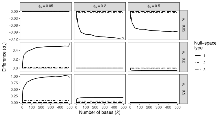
Figure 1: Adjusted vs unadjusted OLS models: amount of bias reduction or amplification, quantified by the difference $d_{x}$, for increasing number of bases in $\mathbf{B}$ and for several combinations of range parameters. Each line type represents a type of null space used to construct $\mathbf{B}$. Note that the scales on the y-axes are different for each “row”.

In summary, adopting the type-1 null space seems to provide the best results in terms of confounding bias mitigation, since the exposure and the bases are not orthogonal, making it possible to capture the correlation between $\mathbf{X}$ and $\mathbf{W}$. For this reason, in what follows we only consider type-1 null space. However, we seek for a parsimonious model that allows for the selection of the most important bases, therefore in the next Section we propose a regularization strategy.

5 Proposed Regularization of the Regression Model

We consider Equation (9) as the likelihood function. As inference is performed following the Bayesian paradigm, a key aspect of model specification is the prior distribution for the coefficients of the basis functions. We propose using spike-and-slab priors (George and McCulloch, 1997), extensively adopted to identify the most important covariates associated with the outcome, and to estimate posterior model probabilities (Fontanella et al., 2019c). These priors offer a flexible alternative to truncation (Morris, 2015), allowing to explore all possible models within a hierarchical formulation, at a minimal computational cost. Also, a parsimonious model is obtained through sparsity, the regularization mechanism of free-knot splines (Morris, 2015), and the shrinkage process is controlled by defining only very few hyperparameters (Fontanella et al., 2019c). In what follows, we consider three different Bayesian hierarchical models.

Spike-and-slab with fixed-variance model (SS_fv)

Following George and McCulloch (1997), it is assumed that $\xi_{j}$ follows a prior distribution given by a mixture of normals, namely:

$$\xi_{j}|\gamma_{j},\psi_{j}^{2} \stackrel{{\scriptstyle ind}}{{\sim}}\gamma_{j}N(0,\psi_{j}^{2})+(1-\gamma_{j})N(0,c_{0}\psi_{j}^{2})\,,\quad\mbox{for }j=1,\dots,p$$

$$\gamma_{j}|w \sim Ber(w)\,,$$

where $\gamma_{j}$ is an indicator variable, $\psi_{j}^{2}$ denotes the fixed prior variance assigned to the slab components, and $c_{0}$ is a small number such that $c_{0}\psi_{j}^{2}$ defines the prior variance for the spike components. The probability of a large prior variance being assigned to a basis coefficient is assumed fixed, $w=0.5$, but it is also possible to consider a beta prior distribution such that $w\sim Beta(a_{w},b_{w})$ with usually $a_{w}=b_{w}=1$ (Ishwaran and Rao, 2005).

For the fixed effects ($\beta_{0}$ and $\beta_{x}$) we assign independent, zero mean, normal prior distribution with known variance $V_{\beta}$, and the for the nugget effect ($\tilde{\sigma}_{\epsilon}^{2}$) we assign an inverse-gamma prior with known parameters $a$ and $b$. Hence, the parameter vector containing all the unknowns is $\bm{\Theta}=(\bm{\beta}^{\prime},\bm{\xi}^{\prime},\tilde{\sigma}_{\epsilon}^{2},\{\gamma_{j}\}_{j=1}^{p})$.

Spike-and-slab with normal mixture of inverse gamma model (SS_nmig)

The second option considered is based on a normal mixture of inverse gamma (NMIG) priors. This allows for more flexibility, since a prior distribution for $\psi_{j}^{2}$ is introduced as an additional stage in the hierarchy, such that $\psi_{j}^{2}\sim IG(a_{\psi},b_{\psi})$ (Ishwaran and Rao, 2005, Scheipl et al., 2012), and the unknown parameter vector becomes $\bm{\Theta}=(\bm{\beta}^{\prime},\bm{\xi}^{\prime},\tilde{\sigma}_{\epsilon}^{2},\{\gamma_{j}\}_{j=1}^{p},\{\psi_{j}^{2}\}_{j=1}^{p})$.

Spike-and-slab with product moment model (SS_mom)

The two options outlined above are examples of local prior structures, in the sense that the prior density of any expansion coefficient is concentrated around zero. However, if a basis is selected by the model because of its importance, its associated coefficient cannot be null. Therefore, non-local prior structures assign most of the prior probability mass away from zero for any slab component. For high-dimensional regression settings, classes of non-local priors are proposed by Johnson and Rossell (2012) and Rossell and Telesca (2017), with the main advantage of not demanding a high computational cost. In this paper, we consider the first-order product moment (pMOM) priors, according to which any $\xi_{j}$ can be considered as a mixture between a point mass at zero and the following density:

$$\xi_{j}|\tilde{\sigma}_{\epsilon}^{2},M_{t}\stackrel{{\scriptstyle ind}}{{\sim}}\frac{\xi_{j}^{2}}{\nu\tilde{\sigma}_{\epsilon}^{2}}N\left(0,\nu\tilde{\sigma}_{\epsilon}^{2}\right)\,,$$

where $\nu$ is a scale parameter. Additionally, we assume a Beta-Binomial prior on $M_{t}$ following Johnson and Rossell (2012) and Rossell and Telesca (2017). Hence, the vector $\bm{\Theta}$ is similar to that of the SS_fv model, with $\{\gamma_{j}\}_{j=1}^{p}$ replaced by the parameters defining the prior distribution on the model space.

Inference Procedure

The posterior distribution of $\bm{\Theta}$, under each model, is proportional to the likelihood times the prior distribution. To perform posterior inference under SS_fv and SS_nmig models, we develop a Markov chain Monte Carlo (MCMC) scheme, while for the SS_mom model we utilize the package mombf within the R software (R Core Team, 2023, Rossell et al., 2023). All the computational details to implement the inference procedure are reported in Web Appendix B.

6 Simulation Study

We conduct an extensive simulation study to shed light on the ability of our proposed approach (abbreviated as SS) to mitigate the spatial confounding bias, and to compare it to other methods in the literature. The data, sampled from a $64\times 64$ grid over the unit square, are generated by fixing $\delta=0.5$ and $\sigma_{x}^{2}=1$, and by considering three combinations of range parameters, namely $\phi_{x}=0.05,\phi_{w}=0.5$ (we refer to this combination as Configuration I), $\phi_{x}=0.5,\phi_{w}=0.05$ (Configuration II), and $\phi_{x}=0.2,\phi_{w}=0.2$ (Configuration III). These combinations are selected based on the findings in Paciorek (2010) and Page et al. (2017), so it is expected that the spatial confounding bias is mitigated in Configuration I, amplified in Configuration II, and not affected in Configuration III. In each configuration, the exposure is generated only once, then conditional on it, we sample $\mathbf{W}_{x}$ and the outcome, $\mathbf{Y}$, to obtain 100 different replicates. We set $\bm{\beta}=(1,2)^{\prime}$ and $\sigma_{\epsilon}^{2}=0.25$. To make comparisons across configurations, we consider $n=500$ randomly-sampled locations as fixed, and we set the relative OLS bias (i.e. the ratio $\Delta_{OLS}/\beta_{x}$) to $0.15$. Therefore, given $\delta$, we allow $\sigma_{w}^{2}$ to vary accordingly. The methods we compare our proposed approach with are reported in Table 1.

Table 1: Competing approaches analyzed in the simulation study.

Method	Description	Reference
OLS	The unadjusted non-spatial model, fitted using ordinary least squares.
SRE (spatial random effect)	The spatial linear model in Equation (1) where $W(\mathbf{s}_{i})$ is an Gaussian process with exponential covariance function, independent of the exposure.
SpatialTP	The model where $W(\mathbf{s}_{i})$ is approximated by a basis expansion from a thin-plate regression spline (TPRS) evaluated at the data locations.	Dupont et al. (2022)
gSEM (geoadditive Structural Equation Model)	The model where the spatial dependence is regressed away from both the response and the exposure through the use of TPRS. Then, a regression involving the residuals is used to estimate the exposure effect.	Thaden and Kneib (2018), Dupont et al. (2022)
Spatial+	The model where the spatial dependence is regressed away only from the exposure. Then, the outcome is regressed on the residuals and on a smooth term. A penalty parameter is estimated using generalized cross-validation.	Dupont et al. (2022)
Spatial+_fx	The Spatial+ model where the penalty parameter is fixed at zero.	Dupont et al. (2022)
KS (Keller-Szpiro)	This approach consists in: (i) regressing the outcome on a matrix of TPRS basis functions, with its degrees of freedom found by minimizing the Akaike information criterion (AIC); (ii) fitting a SpatialTP model where the TPRS has exactly the pre-selected degrees of freedom.	Keller and Szpiro (2020)
SA (spectral adjustment)	The model where a basis expansion of B-splines constructed in the spectral domain and a Gaussian process, independent of the other covariates, are included in the model specification.	Guan et al. (2023)

To avoid scale issues, all variables are standardized, but for ease of interpretation, results are shown on the original scale of the coefficients. The following values are adopted for the hyperparameters in the model: $V_{\beta}=1$, $a=2$, $b=0.1$, $c_{0}=10^{-4}$. We also set $\psi_{j}^{2}=1$ for FV priors, or $a_{\psi}=2$ and $b_{\psi}=1$ for NMIG priors. In the pMOM case, $\nu=0.348$ is the suggested default value (Johnson and Rossell, 2012).

6.1 Results

For each configuration and each model, Figure 2 depicts a boxplot based on 100 estimates of the exposure effect. For the models fitted under the Bayesian paradigm (i.e., SRE, SA and SS), the Bayesian estimator is the posterior mean. The MCMC algorithms are run for a total of 30,000 iterations, with a thinning of 5, where the first 10,000 draws are discarded.

The top panel of Figure 2 illustrates a common scenario in practice where the exposure is less smooth than the unmeasured confounder (Configuration I). Whereas Spatial+_fx provides estimates that are on average the closest to the true value for $\beta_{x}$ (which is depicted as a red dashed line), all three versions of SS are able to reduce the bias similarly. In the middle panel (Configuration II), the confounding bias is usually amplified, however SS_mom nearly reproduces the non-spatial model’s estimates. This may be due to the regularization and model selection scheme implied by the pMOM priors. Indeed, just one basis is selected on average with a posterior inclusion probability greater than $0.5$. Furthermore, for each one of the 100 replicates, SS_mom produces estimates that are closer to the true simulated $\beta_{x}$ than those obtained by the competing approaches. In particular, it is worth noting that now Spatial+_fx, which performed best in Configuration I, always amplifies the bias more than SS_mom. In the bottom panel (Configuration III), it seems that most of the approaches produce estimators as biased as the one of the non-spatial model, so nothing could be concluded about the presence of spatial confounding. However, note that this configuration is rather unrealistic in practice.

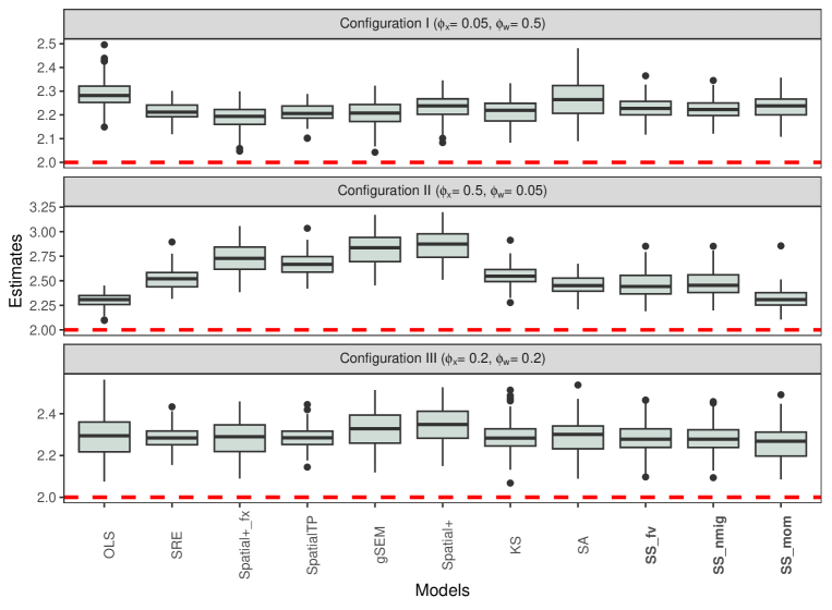
Figure 2: Boxplots representing the estimated exposure effect for the models in the simulation study, under three configurations where different values are assigned to the range parameters, $\phi_{x}$ and $\phi_{w}$. The red dashed line represents the real value, $\beta_{x}=2$.

In Web Appendix C, we show, for the three configurations, that the median correlation between the bases selected with high posterior inclusion probability and $W_{x}(\cdot)$ is generally greater than $0.5$, and that the difference $d_{x}$ (given the selected bases) is always smaller or equal to zero under pMOM priors. Furthermore, Web Appendix C reports other simulation scenarios, where we also vary $\delta$ and $\sigma_{x}^{2}$.

7 Reducing Confounding Bias in Ozone–NO_x Association

We apply the proposed model to an environmental dataset concerning tropospheric ozone (O₃). This greenhouse gas poses risks to both human health and the environment when present in the troposphere. For example, it may cause respiratory diseases, or permanently damage lung tissue. Additionally, it has the potential to harm agricultural crops and forests (Nguyen et al., 2022). This gas is not directly emitted, but rather forms through chemical reactions between nitrogen oxides (NO_x) and volatile organic compounds (VOCs), in the presence of sunlight and high temperatures. Consequently, ozone concentrations typically peak during daytime in summer (Nguyen et al., 2022, Nussbaumer et al., 2022).

Our aim is to infer on the relationship between O₃ and nitrogen oxides from June to August 2019 in three Italian regions, namely Lazio, Abruzzo and Molise. NO_x is made up of nitrogen oxide (NO) and nitrogen dioxide (NO₂), and is released into the atmosphere from combustion sources (e.g., industrial facilities and motor vehicles). We employ the following linear model, where we also control for meteorological variables since they are potential confounders (Chen et al., 2020, Nguyen et al., 2022, Silva and Pires, 2022):

$$\begin{split}log(O_{3}(\mathbf{s}_{i}))&=\beta_{1}^{o}log(NO_{x}(\mathbf{s}_{i}))+\beta_{2}^{o}u_{10}(\mathbf{s}_{i})+\beta_{3}^{o}v_{10}(\mathbf{s}_{i})+\beta_{4}^{o}Temp(\mathbf{s}_{i})+\beta_{5}^{o}SSR(\mathbf{s}_{i})\\ &+\beta_{6}^{o}VOC(\mathbf{s}_{i})+\beta_{7}^{o}RH(\mathbf{s}_{i})+\epsilon^{o}(\mathbf{s}_{i})\,,\qquad i=1,\dots,n\,,\end{split}$$ (13)

where $\epsilon^{o}(\mathbf{s}_{i})\stackrel{{\scriptstyle iid}}{{\sim}}N(0,\sigma_{\epsilon^{o}}^{2})$ and $log(O_{3}(\mathbf{s}_{i}))$ is the natural logarithm of ozone concentrations (in $\mu g/m^{3}$). The covariates represent, in the order, the natural logarithm of NO_x concentrations (in $\mu g/m^{3}$), eastward and northward components of the wind at a height of 10 meters above Earth’s surface (in $m/s$), air temperature at 2 meters above Earth’s surface (in $K$), surface net solar radiation (in $J/m^{2}$), volatile organic compounds (in $\mu g/m^{3}$), and relative humidity (RH, expressed as percentage).

We collected hourly remote-sensed measurements of NO, NO₂, VOC, and O₃ concentrations, on a 0.1° regular latitude-longitude grid, from the Copernicus Atmosphere Monitoring Service (CAMS) Atmosphere Data Store (INERIS et al., 2022). We considered only the time span between 8 a.m. and 6 p.m., while the grid points are $n=353$. A similar procedure is followed to gather meteorological variables, with data available at the same spatial resolution from the ERA5-Land reanalysis dataset within the Copernicus Climate Change Service (C3S) Climate Data Store (Muñoz Sabater, 2019). RH is not directly available from the ERA5-Land dataset, so it was derived from dew-point temperature at 2 meters above Earth’s surface (DT) using the August-Roche-Magnus approximation formula (Alduchov and Eskridge, 1996): $RH=100\times\exp\left(\frac{17.625\times DT}{243.04+DT}-\frac{17.625\times Temp}{243.04+Temp}\right)$.

The OLS method is used to fit the “full” model in Equation (13), whose estimate indicates that a $1\%$ increase in NO_x concentration is associated with a $0.021\%$ increase in O₃ on average (95% confidence interval: $[0.005\%,0.038\%]$). To account for possible residual autocorrelation, we also fit a spatial linear model, which provides the same estimate for $\beta_{1}^{o}$. Then, following Paciorek (2010), to explore how the results would have changed if the potential confounders were not observed, we fit a model where the exposure is the only covariate. The results obtained by all the approaches previously considered are depicted in Figure 3. The estimate for the non-spatial model, labeled “OLS” in the figure, has increased to $0.076\%$ (95% confidence interval: $[0.063\%,0.088\%]$) as a result of spatial confounding.

Using the OLS estimates from the “full” model, we obtain an estimate of the unmeasured confounder. We then compare the spatial range of the exposure and the unmeasured confounder by fitting spatial linear models on them. Based on the posterior means of the parameters, it seems that NO_x has a smaller spatial range. Therefore, given the similarity with Configuration I (see Section 6), we expect a reduction of bias. Indeed, the estimates from the competing methods are closer to the estimates from the “full” model. In Configuration I, Spatial+_fx achieved the greatest reduction in bias, but in this application its 95% confidence interval contains the zero. On the other hand, the credible intervals of our proposed approach are bounded away from zero.

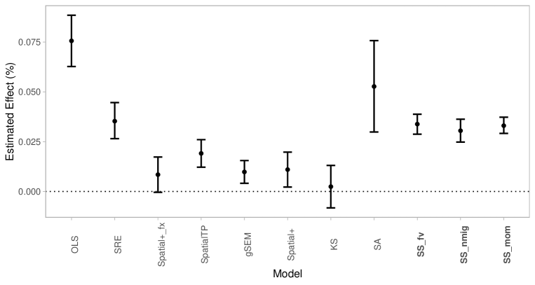
Figure 3: Estimated effects (and respective 95% intervals) of NO_x on O₃, under different models. “OLS” refers to the model where all potential confounders are excluded.

8 Discussion

In this paper, a novel approach to mitigate the issue of spatial confounding has been proposed. We have exploited the principal spline representation of the latent spatial structure, where the basis functions, constructed based on the spectral decomposition of a spatial potential function matrix (Mardia et al., 1996), can be envisioned as proxy variables for the spatially-varying unmeasured confounder. Within the reduced-rank representation of the spatial linear model, we have demonstrated the relationship between the bias from the adjusted OLS model and that from the non-spatial OLS model, which holds for any basis expansion. Reflecting the findings in Paciorek (2010), we state that spatial confounding can be mitigated only when the spatial range of the exposure ($\phi_{x}$) is smaller than that of the unmeasured confounder ($\phi_{w}$). However, if the bases are orthogonal to the exposure, $d_{x}$ in Equation (12) is null (i.e., the bias equals that of the non-spatial model), regardless of the number of bases included.

Our proposed approach involves imposing spike-and-slab priors on the expansion coefficients. This approach is inherently flexible and allows for the selection of the best proxies from the given set of principal functions. We conducted an extensive simulation and comparison study, which is the first of its kind. Based on the results in Section 6 and in Web Appendix C, SS_mom performs best when $\phi_{x}<\phi_{w}$ (see Configuration I), and it demonstrates greater robustness against bias amplification when $\phi_{x}>\phi_{w}$ (Configuration II) compared to the competing approaches. For example, Spatial+_fx and SS_mom respectively showed a bias reduction of $0.10$ and $0.06$ in Configuration I, but in Configuration II the bias amplification is equal to $0.43$ and $0.02$, respectively. We additionally note that pMOM priors typically produce more parsimonious models than fixed-variance or NMIG priors, and that, regardless of the prior structure, the number of bases selected with high posterior inclusion probability increases when the partial sill of the unmeasured confounder increases. This is consistent with the fact that there is more residual spatial variability to explain. Moreover, Web Appendix C shows that the selected bases provide a low-rank representation that is highly correlated with the unmeasured confounder.

It is worth noting that gSEM, Spatial+, KS and SA require at least two steps to estimate the exposure effect. However, the propagation of uncertainty in parameter estimation from one step to another should be taken into account (Schmidt, 2022). In contrast, our method is a one-step approach and thus bypasses this issue. Moreover, it can deal with data collected from irregularly-spaced locations, unlike the SA model, which requires the exposure to be observed on a grid (Guan et al., 2023).

We have inferred on the association between NO_x and O₃, and we have seen that not accounting for potential confounders largely distorts inferential results, with an OLS estimate that is $3.6$ times larger. However, we are aware that the “full” model may not recover the true exposure–outcome association. The application was only intended to show that our proposed approach can successfully mitigate bias in real-world data settings.

Finally, if the goal is to alleviate the impact of spatial confounding on the exposure–outcome association, we proved that it can be achieved by using low-rank models under the conditions discussed above, that is if $\phi_{x}<\phi_{w}$ and the bases are correlated with the exposure. From a practical viewpoint, our proposal serves as a valuable tool for confounding bias mitigation, and can be used to select the most appropriate model for the data at hand.

Supplementary Materials

The R code to reproduce the analyses is available at https://github.com/czaccard/spatial_confounding_SS.git.

Appendix A Derivation of Difference Between Unadjusted and Adjusted OLS Estimators

Consider a more compact form for the semi-parametric model:

$$\mathbf{Y}=\tilde{\mathbf{X}}\bm{\beta}+\mathbf{B}\bm{\xi}+\tilde{\bm{\epsilon}}=\mathbf{A}\bm{\theta}+\tilde{\bm{\epsilon}}\,,$$ (14)

where $\mathbf{A}=\begin{bmatrix}\tilde{\mathbf{X}}&\mathbf{B}\end{bmatrix}$ indicates the $n\times(p+2)$ full design matrix where $\tilde{\mathbf{X}}$ and $\mathbf{B}$ are bound column-wise, and $\bm{\theta}=(\bm{\beta}^{\prime},\bm{\xi}^{\prime})^{\prime}$ is the associated vector of coefficients.

The expected value of the adjusted OLS estimator is:

$$E\left[\hat{\bm{\theta}}_{OLS}|\mathbf{X=x}\right] =(\mathbf{A^{\prime}A})^{-1}\mathbf{A}^{\prime}E\left[\mathbf{Y}|\mathbf{X=x}\right]$$

$$=(\mathbf{A^{\prime}A})^{-1}\mathbf{A}^{\prime}\left[\tilde{\mathbf{X}}\bm{\beta}+\bm{\mu}_{w|x}\right]$$

$$=(\mathbf{A^{\prime}A})^{-1}\mathbf{A}^{\prime}\tilde{\mathbf{X}}\bm{\beta}+\delta\frac{\sigma_{w}}{\sigma_{z}}(\mathbf{A^{\prime}A})^{-1}\mathbf{A}^{\prime}\mathbf{R}_{\phi_{w}}^{1/2}\mathbf{R}_{\phi_{x}}^{-1/2}\mathbf{x}$$

We will consider only the first two elements of this expectation vector in what follows. The first term in the expression above gives $\bm{\beta}$, as expected. The second term refers to the bias, which we indicate as $\Delta_{adj}$.

Since $\mathbf{A^{\prime}A}$ is a block matrix, it follows that:

$$(\mathbf{A^{\prime}A})^{-1}=\left[\begin{array}[]{cc}\tilde{\mathbf{X}}^{\prime}\tilde{\mathbf{X}}&\tilde{\mathbf{X}}^{\prime}\mathbf{B}\\ \mathbf{B}^{\prime}\tilde{\mathbf{X}}&\mathbf{B}^{\prime}\mathbf{B}\\ \end{array}\right]^{-1}=\left[\begin{array}[]{cc}\mathbf{Q}&-\mathbf{T}\\ \bm{\Xi}&\mathbf{S}^{-1}\\ \end{array}\right]$$ (15)

and

$$\Delta_{adj}=\delta\frac{\sigma_{w}}{\sigma_{z}}(\mathbf{Q\tilde{X}}^{\prime}-\mathbf{TB}^{\prime})\mathbf{R}_{\phi_{w}}^{1/2}\mathbf{R}_{\phi_{z}}^{-1/2}\mathbf{x}\,,$$

where $\mathbf{Q}=(\mathbf{\tilde{X}^{\prime}\tilde{X}})^{-1}+\mathbf{TB^{\prime}\tilde{X}}(\mathbf{\tilde{X}^{\prime}\tilde{X}})^{-1}$, $\mathbf{T}=(\mathbf{\tilde{X}^{\prime}\tilde{X}})^{-1}\mathbf{\tilde{X}^{\prime}BS}^{-1}$, $\bm{\Xi}=-\mathbf{S}^{-1}\mathbf{B^{\prime}\tilde{X}}(\mathbf{\tilde{X}^{\prime}\tilde{X}})^{-1}$, and $\mathbf{S}=\mathbf{B^{\prime}B-B^{\prime}\tilde{X}}(\mathbf{\tilde{X}^{\prime}\tilde{X}})^{-1}\mathbf{\tilde{X}^{\prime}B}$.

With some algebra, it turns out that

$$\Delta_{adj} =\delta\frac{\sigma_{w}}{\sigma_{z}}\left[(\mathbf{\tilde{X}^{\prime}\tilde{X}})^{-1}\mathbf{\tilde{X}}^{\prime}+\mathbf{TB^{\prime}\tilde{X}}(\mathbf{\tilde{X}^{\prime}\tilde{X}})^{-1}\mathbf{\tilde{X}}^{\prime}-\mathbf{TB^{\prime}}\right]\mathbf{R}_{\phi_{w}}^{1/2}\mathbf{R}_{\phi_{z}}^{-1/2}\mathbf{x}$$

$$=\delta\frac{\sigma_{w}}{\sigma_{z}}(\mathbf{\tilde{X}^{\prime}\tilde{X}})^{-1}\mathbf{\tilde{X}}^{\prime}\mathbf{R}_{\phi_{w}}^{1/2}\mathbf{R}_{\phi_{z}}^{-1/2}\mathbf{x}+\delta\frac{\sigma_{w}}{\sigma_{z}}\left[\mathbf{TB^{\prime}\tilde{X}}(\mathbf{\tilde{X}^{\prime}\tilde{X}})^{-1}\mathbf{\tilde{X}}^{\prime}-\mathbf{TB^{\prime}}\right]\mathbf{R}_{\phi_{w}}^{1/2}\mathbf{R}_{\phi_{z}}^{-1/2}\mathbf{x}$$

$$=\Delta_{OLS}+\delta\frac{\sigma_{w}}{\sigma_{z}}\mathbf{TB^{\prime}}\left[\mathbf{\tilde{X}}(\mathbf{\tilde{X}^{\prime}\tilde{X}})^{-1}\mathbf{\tilde{X}}^{\prime}-\mathbf{I}_{n}\right]\mathbf{R}_{\phi_{w}}^{1/2}\mathbf{R}_{\phi_{x}}^{-1/2}\mathbf{x}$$

$$=\Delta_{OLS}+\left[\begin{array}[]{c}d_{0}\\ d_{x}\end{array}\right]$$

We have discussed three null space types, from which different forms of $\mathbf{U}$ will derive:

1. $\mathbf{U}=\begin{bmatrix}1&\mathbf{s}_{1}[1]&\mathbf{s}_{1}[2]\\ &\vdots&\\ 1&\mathbf{s}_{n}[1]&\mathbf{s}_{n}[2]\end{bmatrix}$

2. $\mathbf{U}=\begin{bmatrix}1&X(\mathbf{s}_{1})&\mathbf{s}_{1}[1]&\mathbf{s}_{1}[2]\\ &\vdots&\vdots&\\ 1&X(\mathbf{s}_{n})&\mathbf{s}_{n}[1]&\mathbf{s}_{n}[2]\end{bmatrix}$

3. $\mathbf{U}=\mathbf{\tilde{X}}$

Consider the second type, and let $\mathbf{C}$ denote the matrix collecting easting and northing coordinates of the $n$ sampling locations, and let $\mathbf{F}^{*}$ be the matrix containing the eigenvectors corresponding to the non-null eigenvalues. Therefore, it follows that $\mathbf{A}=\left[\begin{array}[]{ccc}\tilde{\mathbf{X}}&\mathbf{C}&\mathbf{F}^{*}\end{array}\right]$, and $\mathbf{B}=\mathbf{F}^{*}$.

The components of the block inverse in Equation (15) become:

$$\mathbf{S} =\mathbf{I}_{n-q},\quad q=4$$

$$\mathbf{T} =\mathbf{0}$$

$$\mathbf{Q} =\left[\begin{array}[]{cc}\mathbf{\tilde{X}^{\prime}\tilde{X}}&\mathbf{\tilde{X}^{\prime}C}\\ \mathbf{C^{\prime}\tilde{X}}&\mathbf{C^{\prime}C}\\ \end{array}\right]$$

Because of the orthogonality between $\left[\begin{array}[]{cc}\tilde{\mathbf{X}}&\mathbf{C}\end{array}\right]$ and $\mathbf{F}^{*}$, it turns out that $\Delta_{adj}$ does not depend on the bases in $\mathbf{F^{*}}$ anymore:

$$\Delta_{adj} =\Delta_{OLS}$$

$$+\delta\frac{\sigma_{w}}{\sigma_{z}}\Bigl{\{}(\mathbf{\tilde{X}^{\prime}\tilde{X}})^{-1}\mathbf{\tilde{X}}^{\prime}\mathbf{C}\left[\mathbf{C}^{\prime}(\mathbf{I}_{n}-\mathbf{\tilde{X}}(\mathbf{\tilde{X}^{\prime}\tilde{X}})^{-1}\mathbf{\tilde{X}^{\prime}})\mathbf{C}\right]^{-1}\mathbf{C}^{\prime}\mathbf{\tilde{X}}(\mathbf{\tilde{X}^{\prime}\tilde{X}})^{-1}\mathbf{\tilde{X}}^{\prime}$$

$$-\left[\mathbf{X}^{\prime}(\mathbf{I}_{n}-\mathbf{C}(\mathbf{C^{\prime}C})^{-1}\mathbf{C^{\prime}})\mathbf{\tilde{X}}\right]^{-1}\mathbf{\tilde{X}}^{\prime}\mathbf{C}(\mathbf{C^{\prime}C})^{-1}\mathbf{C^{\prime}}\Bigr{\}}\mathbf{R}_{\phi_{w}}^{1/2}\mathbf{R}_{\phi_{z}}^{-1/2}\mathbf{x}\,,$$

so the confounding bias can be reduced only through the inclusion of the spatial coordinates in the model.

In the case of type-3 null space, it results that $\mathbf{A}=\left[\begin{array}[]{cc}\tilde{\mathbf{X}}&\mathbf{F}^{*}\end{array}\right]$, $\mathbf{B}=\mathbf{F}^{*}$ and that

$$\mathbf{S} =\mathbf{I}_{n-q},\quad q=2$$

$$\mathbf{T} =\mathbf{0}$$

$$\mathbf{Q} =(\mathbf{\tilde{X}^{\prime}\tilde{X}})^{-1}$$

Thus, $\Delta_{adj}=\Delta_{OLS}$ and there is no confounding adjustment.

Appendix B Derivation of the Full Conditional Distributions

The Gibbs sampler Gelfand (2000) is implemented using the following full conditional distributions. Starting from Equation (14), the prior variance of the regression coefficients, $\mathbf{V}_{\bm{\theta}}$, is a diagonal matrix with first two elements equal to $V_{\beta}$, and $(j+2)$th element given by $Var\left[\xi_{j}|\gamma_{j},\psi_{j}^{2}\right]$. The symbol $\bullet$ denotes data and all the parameters except for the parameter that is being updated.

$$\gamma_{j}|\bullet \sim Ber\left(\frac{m_{1j}}{m_{1j}+m_{0j}}\right)\,,\quad\mbox{for }j=1,\dots,n$$

$$\psi_{j}^{2}|\bullet \sim IG\left(a_{\psi}+\frac{1}{2},b_{\psi}+\frac{\xi_{j}^{2}}{2[\gamma_{j}+(1-\gamma_{j})c_{0}]}\right)\mbox{ (only for NMIG priors)}$$

$$\tilde{\sigma}_{\epsilon}^{2}|\bullet \sim IG\left(a+\frac{n}{2},b+\frac{1}{2}(\mathbf{y}-\mathbf{A}\bm{\theta})^{\prime}(\mathbf{y}-\mathbf{A}\bm{\theta})\right)$$

$$\bm{\theta}|\bullet \sim N\left(\tilde{\sigma}_{\epsilon}^{-2}\mathbf{V}\mathbf{A}^{\prime}\mathbf{y},\mathbf{V}\right)\,,$$

where $\mathbf{V}^{-1}=\left(\tilde{\sigma}_{\epsilon}^{-2}\mathbf{A}^{\prime}\mathbf{A}+\mathbf{V}_{\bm{\theta}}^{-1}\right)$ and

$$m_{1j} \propto w\exp\left[-\frac{\xi_{j}^{2}}{2\psi_{j}^{2}}\right]\,,$$

$$m_{0j} \propto(1-w)\frac{1}{\sqrt{c_{0}}}\exp\left[-\frac{\xi_{j}^{2}}{2c_{0}\psi_{j}^{2}}\right]\,.$$

In the pMOM case, posterior estimation of $\xi_{j}$’s requires finding the regions in the model space with high posterior probability, introducing a latent variable and sampling from a truncated Gaussian distribution. We refer to the work by Rossell and Telesca (2017) for further details about the MCMC algorithm, which is available in the R package mombf (R Core Team, 2023, Rossell et al., 2023).

Appendix C Additional Findings from the Simulation Study

C.1 Difference Between Unadjusted and
Adjusted OLS Estimators

In Section 3.2 of the main manuscript, we have analyzed how $d_{x}$ changed by progressively increasing the number of bases, $k$, but it is possible to repeat the experiments by considering the covariates selected during each MCMC iteration with posterior inclusion probability $>0.5$. For each configuration, boxplots of the values of $d_{x}$ over the 100 replicates are represented in the top row of Figure 4 for the three types of spike-and-slab priors. Note that the values of $d_{x}$ may not exactly match the bias reduction or amplification from the corresponding configuration, because the regularization induced by the priors was not taken into consideration in Section A. Nonetheless, using the pMOM priors we generally obtain values of $d_{x}$ that are negative or close to zero in the worst scenarios: this is because no bases are usually selected when there is risk to amplify the confounding bias.

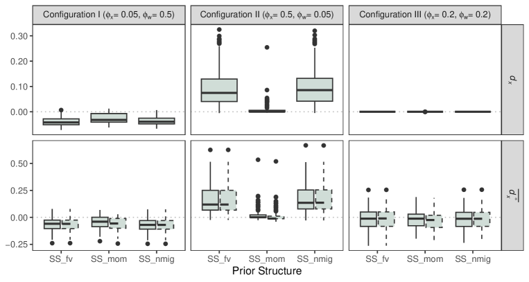
Figure 4: For each configuration and for each prior structure, boxplots of a posteriori analysis of the amount of bias reduction or amplification are depicted, given the bases selected after each MCMC step. The top panels depict $d_{x}$, while the bottom panels $\overline{d_{x}^{*}}$. The latter is calculated using both analytic (solid lines) and empirical (dashed lines) formulae. Note that the scales on the y-axes are different for each “row”.

C.2 Difference Between Bayesian and
Frequentist Estimators

The foregoing analysis has not taken into consideration how the prior distributions assumed on the basis coefficients impact on the confounding bias. Following a reasoning similar in spirit to that of Hans (2009), it is possible to compare the unadjusted OLS estimator with the mean of the posterior distribution of $\beta_{x}$, when the bases are included. For notational convenience, let the latter quantity be denoted as $\bm{\beta}_{post}=E[\bm{\beta}|\bullet]$. We demonstrate that their difference, $d_{x}^{*}=\bm{\beta}_{post}-\hat{\bm{\beta}}_{OLS}$, is equal to the second element of the following vector:

$$\left[\begin{array}[]{c}d_{0}^{*}\\ d_{x}^{*}\end{array}\right]=\mathbf{TB^{\prime}}(\hat{\mathbf{Y}}_{OLS}-\mathbf{Y})/\tilde{\sigma}_{\epsilon}^{2}\,,$$ (16)

where $\hat{\bm{\beta}}_{OLS}$ and $\hat{\mathbf{Y}}_{OLS}=\tilde{\mathbf{X}}\hat{\bm{\beta}}_{OLS}$ are, respectively, the estimate and the vector of fitted values under the unadjusted OLS model, but now $\mathbf{T}$ is not the same as before since it derives from the inversion of another block matrix which depends on the priors.

Proof.

Starting again from Equation (14), now the expected value of the conditional posterior of $\bm{\theta}$ is of interest. If non-informative independent priors are assumed on all the parameters, we have:

$$E\left[\bm{\theta}|\bullet\right]=\left(\mathbf{A^{\prime}A}/\tilde{\sigma}_{\epsilon}^{2}+\mathbf{V}_{\bm{\theta}}^{-1}\right)^{-1}\mathbf{A^{\prime}y}/\tilde{\sigma}_{\epsilon}^{2}$$

where

$$\mathbf{V}_{\bm{\theta}}^{-1}=\left[\begin{array}[]{cc}\mathbf{V}_{\bm{\beta}}^{-1}&\mathbf{0}\\ \mathbf{0}&\mathbf{V}_{\bm{\xi}}^{-1}\\ \end{array}\right]\,.$$

Since we use non-informative priors on $\bm{\beta}$, the upper-left block of $\mathbf{V}_{\bm{\theta}}^{-1}$ tends to the null matrix, thus:

$$\left(\mathbf{A^{\prime}A}/\tilde{\sigma}_{\epsilon}^{2}+\mathbf{V}_{\bm{\theta}}^{-1}\right)^{-1} \approx\left[\begin{array}[]{cc}\mathbf{\tilde{X}^{\prime}\tilde{X}}/\tilde{\sigma}_{\epsilon}^{2}&\mathbf{\tilde{X}^{\prime}B}/\tilde{\sigma}_{\epsilon}^{2}\\ \mathbf{B^{\prime}\tilde{X}}/\tilde{\sigma}_{\epsilon}^{2}&\mathbf{B^{\prime}B}/\tilde{\sigma}_{\epsilon}^{2}+\mathbf{V}_{\bm{\xi}}^{-1}\\ \end{array}\right]^{-1}=$$

$$=\left[\begin{array}[]{cc}\mathbf{Q}&-\mathbf{T}\\ \bm{\Xi}&\mathbf{S}^{-1}\\ \end{array}\right]$$

where

$$\mathbf{S}=\mathbf{B^{\prime}B}/\tilde{\sigma}_{\epsilon}^{2}+\mathbf{V}_{\bm{\xi}}^{-1}-\mathbf{B}^{\prime}\mathbf{\tilde{X}}(\mathbf{\tilde{X}^{\prime}\tilde{X}})^{-1}\mathbf{\tilde{X}^{\prime}B}/\tilde{\sigma}_{\epsilon}^{2}\,,$$

$$\mathbf{T}=(\mathbf{\tilde{X}^{\prime}\tilde{X}})^{-1}\mathbf{\tilde{X}^{\prime}BS}^{-1}\,,$$

$$\mathbf{Q}=(\mathbf{\tilde{X}^{\prime}\tilde{X}})^{-1}\tilde{\sigma}_{\epsilon}^{2}+\mathbf{TB^{\prime}\tilde{X}}(\mathbf{\tilde{X}^{\prime}\tilde{X}})^{-1}\,,$$

$$\bm{\Xi}=-\mathbf{S}^{-1}\mathbf{B^{\prime}\tilde{X}}(\mathbf{\tilde{X}^{\prime}\tilde{X}})^{-1}\,.$$

Now we can focus on the first two elements of $\bm{\theta}$, i.e., $\bm{\beta}$, to obtain:

$$\bm{\beta}_{post} =(\mathbf{QX^{\prime}-TB^{\prime}})\mathbf{y}/\tilde{\sigma}_{\epsilon}^{2}$$

$$=\hat{\bm{\beta}}_{OLS}+\mathbf{TB^{\prime}\tilde{X}}\hat{\bm{\beta}}_{OLS}/\tilde{\sigma}_{\epsilon}^{2}-\mathbf{TB^{\prime}Y}/\tilde{\sigma}_{\epsilon}^{2}$$

$$=\hat{\bm{\beta}}_{OLS}+\mathbf{TB^{\prime}}(\hat{\mathbf{Y}}_{OLS}-\mathbf{Y})/\tilde{\sigma}_{\epsilon}^{2}$$

$$=\hat{\bm{\beta}}_{OLS}+\left[\begin{array}[]{c}d_{0}^{*}\\ d_{x}^{*}\end{array}\right]\,.$$

∎

Therefore, $d_{x}^{*}$ can be obtained using either an “empirical formula”, that is as a difference between Bayesian and frequentist estimators, or an “analytic formula”, which depends on the bases, the residuals from the unadjusted OLS fit, and the prior structure assumed on the basis coefficients.

For the type-2 null space, we are not assuming spike-and-slab priors on the spatial coordinates, so a large variance is imposed to the respective coefficients, and the previous formulae can be simplified: from the orthogonality between $\left[\begin{array}[]{cc}\tilde{\mathbf{X}}&\mathbf{C}\end{array}\right]$ and $\mathbf{F}^{*}$, the matrix $\left(\mathbf{A^{\prime}A}/\tilde{\sigma}_{\epsilon}^{2}+\mathbf{V}_{\bm{\theta}}^{-1}\right)$ becomes block-diagonal and its inverse is:

$$\left(\mathbf{A^{\prime}A}/\tilde{\sigma}_{\epsilon}^{2}+\mathbf{V}_{\bm{\theta}}^{-1}\right)^{-1}\approx\left[\begin{array}[]{cc}\tilde{\sigma}_{\epsilon}^{2}\left[\begin{array}[]{cc}\tilde{\mathbf{X}}^{\prime}\tilde{\mathbf{X}}&\mathbf{\tilde{X}^{\prime}C}\\ \mathbf{C^{\prime}\tilde{X}}&\mathbf{C^{\prime}C}\end{array}\right]^{-1}&\mathbf{0}\\ \mathbf{0}&\left(\mathbf{I}_{n-q}/\tilde{\sigma}_{\epsilon}^{2}+\mathbf{V^{*}}_{\bm{\xi}}^{-1}\right)^{-1}\\ \end{array}\right]\,,$$

where $\mathbf{V^{*}}_{\bm{\xi}}$ is $\mathbf{V}_{\bm{\xi}}$ without the first two columns and the first two rows.

It turns out that the posterior mean does not depend on the bases:

$$\bm{\beta}_{post} =\hat{\bm{\beta}}_{OLS}+(\mathbf{\tilde{X}^{\prime}\tilde{X}})^{-1}\mathbf{\tilde{X}}^{\prime}\mathbf{C}\left[\mathbf{C}^{\prime}(\mathbf{I}_{n}-\mathbf{\tilde{X}}(\mathbf{\tilde{X}^{\prime}\tilde{X}})^{-1}\mathbf{\tilde{X}^{\prime}})\mathbf{C}\right]^{-1}\mathbf{C^{\prime}}\hat{\mathbf{Y}}_{OLS}$$

$$-\left[\mathbf{X}^{\prime}(\mathbf{I}_{n}-\mathbf{C}(\mathbf{C^{\prime}C})^{-1}\mathbf{C^{\prime}})\mathbf{\tilde{X}}\right]^{-1}\mathbf{\tilde{X}}^{\prime}\mathbf{C}(\mathbf{C^{\prime}C})^{-1}\mathbf{\tilde{X}^{\prime}}\mathbf{Y}\,,$$

As for the type-3 null space, given the independence between $\mathbf{\tilde{X}}$ and each eigenvector, the posterior mean simplifies to the OLS estimate. In fact:

$$\left(\mathbf{A^{\prime}A}/\tilde{\sigma}_{\epsilon}^{2}+\mathbf{V}_{\bm{\theta}}^{-1}\right)^{-1} \approx\left[\begin{array}[]{cc}\mathbf{\tilde{X}^{\prime}\tilde{X}}/\tilde{\sigma}_{\epsilon}^{2}&\mathbf{0}\\ \mathbf{0}&\mathbf{I}_{n-q}/\tilde{\sigma}_{\epsilon}^{2}+\mathbf{V}_{\bm{\xi}}^{-1}\\ \end{array}\right]^{-1}=$$

$$=\left[\begin{array}[]{cc}(\mathbf{\tilde{X}^{\prime}\tilde{X}})^{-1}\tilde{\sigma}_{\epsilon}^{2}&\mathbf{0}\\ \mathbf{0}&(\mathbf{I}_{n-q}/\tilde{\sigma}_{\epsilon}^{2}+\mathbf{V}_{\bm{\xi}}^{-1})^{-1}\\ \end{array}\right]$$

which implies that $\bm{\beta}_{post}=(\mathbf{\tilde{X}^{\prime}\tilde{X}})^{-1}\mathbf{\tilde{X}^{\prime}Y}=\hat{\bm{\beta}}_{OLS}$.

The bottom panels of Figure 4 show boxplots of $\overline{d_{x}^{*}}=E[d_{x}^{*}|\bullet]$ over the hundred replicates. The results, using both empirical (represented by dashed lines) and analytic (solid lines) formulae, are plotted for each configuration and prior structure. There is an overall correspondence of the results obtained by the formulae, however in the pMOM case a workaround was necessary. Since there is not a closed-form full conditional distribution for the coefficients, it was not possible to derive an analytic formula. Hence, we show what would have happened if the bases in the pMOM case were selected under the fixed-variance prior structure. Again, we do see that the results are consistent with our findings in Section 5 of the paper, and that SS_mom performs better than the other two approaches, since $\overline{d_{x}^{*}}$ is almost always smaller than or equal to zero.

C.3 Correlation Between Unmeasured Confounder and Bases Selected

Another important aspect is whether the selected bases provide a good approximation of the unobserved process. We thus compute the correlation, in absolute terms, between the simulated $\mathbf{w}_{x}$ and the linear combination of bases selected with a posterior inclusion probability $>50\%$, for each replicate and for the three configurations discussed in Section 5 of the paper. Figure 5 represents the results as boxplots, and each panel refers to a configuration. We notice that the median correlation is generally greater than $0.5$, with an exception: in Configuration II, it is approximately $0.2$ under pMOM priors, probably because very few (often none of the) bases have been selected. Besides, it seems that a strong correlation between $\mathbf{W}_{x}$ and the linear combination of bases is a necessary but not sufficient condition. In fact, despite the high correlations, there is no chance to alleviate spatial confounding when exposure and unmeasured confounder have the same spatial range (i.e., Configuration III).

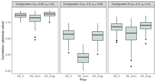
Figure 5: Correlations (in absolute terms) between the basis expansion and the unmeasured confounder, for the three configurations and for each prior structure.

C.4 Other Simulation Scenarios

The following Table 2 reports the results of the simulation study for other configurations not considered in the main manuscript. When $\delta=0$, all the models should provide unbiased estimators for $\beta_{x}$. Unexpectedly, this seems not to be true for gSEM and Spatial+ with estimated smoothing parameter. Then, as $|\delta|$ increases, the confounding bias under any approach increases proportionally. There is an overall symmetry between what happens given negative and positive values for $\delta$, with an exception: the penalized versions of gSEM and Spatial+ tend to produce higher bias if $\delta$ is positive, but smaller (absolute) bias if $\delta$ is negative, when compared to Spatial+_fx (which behaves symmetrically). Next, according to all the models being compared, $\sigma_{x}$ and $\sigma_{w}$ have linear effects on the bias, as expected.

Finally, the number of bases selected by the SS models depends not only on the relationship between the range parameters. Indeed, if the partial sill of the unmeasured confounder increases, the number of bases considered relevant will consequently increase. The reason could be that there is more residual spatial variability to explain. The prior structure also plays an important role, since pMOM priors produce more parsimonious models than FV or NMIG priors.

Table 2: Estimates, averaged over 100 replicates, of $\beta_{x}$ for some other configurations.

$\phi_{x}$	$\phi_{w}$	$\delta$	$\sigma_{x}^{2}$	Null	SRE	Spatial+_fx	SpatialTP	gSEM	Spatial+	KS	SA	SS_fv	SS_nmig	SS_mom
0.20	0.20	0	1.00	2.01	2.00	2.00	2.00	2.05	2.08	1.97	2.01	1.99	2.00	1.97
0.50	0.05	0.2	1.00	2.30	2.55	2.76	2.72	2.86	2.93	2.51	2.53	2.51	2.52	2.37
0.20	0.20	0.2	1.00	2.30	2.28	2.29	2.28	2.33	2.37	2.25	2.29	2.28	2.28	2.25
0.05	0.50	0.2	1.00	2.29	2.20	2.19	2.20	2.19	2.25	2.20	2.21	2.21	2.21	2.21
0.50	0.05	-0.5	1.00	1.71	1.51	1.33	1.37	1.42	1.45	1.46	1.56	1.55	1.54	1.66
0.20	0.20	-0.5	1.00	1.71	1.71	1.72	1.71	1.77	1.80	1.70	1.71	1.71	1.71	1.69
0.05	0.50	-0.5	1.00	1.71	1.78	1.80	1.79	1.82	1.85	1.73	1.73	1.78	1.78	1.75
0.50	0.05	0.5	0.50	2.29	2.47	2.63	2.59	2.77	2.82	2.51	2.39	2.41	2.41	2.30
0.20	0.20	0.5	0.50	2.29	2.28	2.26	2.28	2.34	2.37	2.28	2.27	2.27	2.27	2.26
0.05	0.50	0.5	0.50	2.29	2.22	2.19	2.21	2.22	2.26	2.21	2.28	2.23	2.23	2.24
0.50	0.05	0.5	2.00	2.30	2.57	2.80	2.73	2.86	2.89	2.57	2.52	2.54	2.56	2.35
0.20	0.20	0.5	2.00	2.30	2.29	2.29	2.29	2.32	2.33	2.29	2.30	2.29	2.29	2.26
0.05	0.50	0.5	2.00	2.30	2.21	2.19	2.21	2.20	2.22	2.22	2.24	2.23	2.22	2.22

References

- Alduchov and Eskridge (1996) O. A. Alduchov and R. E. Eskridge. Improved Magnus form approximation of saturation vapor pressure. Journal of Applied Meteorology and Climatology, 35(4):601–609, 1996.
- Azevedo et al. (2021) D. R. Azevedo, M. O. Prates, and D. Bandyopadhyay. MSPOCK: alleviating spatial confounding in multivariate disease mapping models. Journal of Agricultural, Biological and Environmental Statistics, 26:464–491, 2021.
- Banerjee et al. (2014) S. Banerjee, B. P. Carlin, and A. E. Gelfand. Hierarchical modeling and analysis for spatial data. CRC press, 2014.
- CAMS (2023) CAMS. European air quality reanalyses. Copernicus Atmosphere Monitoring Service (CAMS) Atmosphere Data Store (ADS), 2023. URL https://ads.atmosphere.copernicus.eu/cdsapp#!/dataset/cams-europe-air-quality-reanalyses?tab=overview. Accessed on 17-07-2023.
- Chen et al. (2020) L. Chen, J. Zhu, H. Liao, Y. Yang, and X. Yue. Meteorological influences on PM2.5 and O3 trends and associated health burden since China’s clean air actions. Science of the Total Environment, 744:140837, 2020.
- Clayton et al. (1993) D. G. Clayton, L. Bernardinelli, and C. Montomoli. Spatial correlation in ecological analysis. International journal of epidemiology, 22(6):1193–1202, 1993.
- Copernicus Climate Change Service (2023) Copernicus Climate Change Service. ERA5-Land hourly data from 1950 to present. Copernicus Climate Change Service (C3S) Climate Data Store (CDS), 2023. doi: 10.24381/cds.e2161bac. Accessed on 17-07-2023.
- Cressie (1993) N. Cressie. Statistics for spatial data. Wiley series in probability and mathematical statistics. Wiley, New York, rev. edition, 1993. ISBN 9780471002550.
- Duchon (1977) J. Duchon. Splines minimizing rotation-invariant semi-norms in Sobolev spaces. In Constructive Theory of Functions of Several Variables: Proceedings of a Conference Held at Oberwolfach April 25–May 1, 1976, pages 85–100. Springer, 1977.
- Dupont et al. (2022) E. Dupont, S. N. Wood, and N. H. Augustin. Spatial+: a novel approach to spatial confounding. Biometrics, 78(4):1279–1290, 2022.
- Fontanella et al. (2013) L. Fontanella, L. Ippoliti, and P. Valentini. A functional spatio-temporal model for geometric shape analysis. In Advances in Theoretical and Applied Statistics, pages 75–86. Springer, 2013.
- Fontanella et al. (2019a) L. Fontanella, L. Ippoliti, and A. Kume. The offset normal shape distribution for dynamic shape analysis. Journal of Computational and Graphical Statistics, 28(2):374–385, 2019a.
- Fontanella et al. (2019b) L. Fontanella, L. Ippoliti, A. Sarra, E. Nissi, and S. Palermi. Investigating the association between indoor radon concentrations and some potential influencing factors through a profile regression approach. Environmental and Ecological Statistics, 26:185–216, 2019b.
- Fontanella et al. (2019c) L. Fontanella, L. Ippoliti, and P. Valentini. Predictive functional ANOVA models for longitudinal analysis of mandibular shape changes. Biometrical Journal, 61(4):918–933, 2019c.
- Gelfand (2000) A. E. Gelfand. Gibbs sampling. Journal of the American statistical Association, 95(452):1300–1304, 2000.
- George and McCulloch (1997) E. I. George and R. E. McCulloch. Approaches for Bayesian variable selection. Statistica sinica, 33(2):339–373, 1997.
- Guan et al. (2023) Y. Guan, G. L. Page, B. J. Reich, M. Ventrucci, and S. Yang. Spectral adjustment for spatial confounding. Biometrika, 110(3):699–719, 2023.
- Hanks et al. (2015) E. M. Hanks, E. M. Schliep, M. B. Hooten, and J. A. Hoeting. Restricted spatial regression in practice: geostatistical models, confounding, and robustness under model misspecification. Environmetrics, 26(4):243–254, 2015.
- Hans (2009) C. Hans. Bayesian lasso regression. Biometrika, 96(4):835–845, 2009.
- Hodges and Reich (2010) J. S. Hodges and B. J. Reich. Adding spatially-correlated errors can mess up the fixed effect you love. The American Statistician, 64(4):325–334, 2010.
- Hughes and Haran (2013) J. Hughes and M. Haran. Dimension reduction and alleviation of confounding for spatial generalized linear mixed models. Journal of the Royal Statistical Society Series B: Statistical Methodology, 75(1):139–159, 2013.
- INERIS et al. (2022) INERIS, Aarhus University, MET Norway, IEK, I.-N. KNMI, METEO FRANCE, et al. CAMS European air quality forecasts, ENSEMBLE data. Copernicus Atmosphere Monitoring Service (CAMS) Atmosphere Data Store (ADS), 2022. URL https://ads.atmosphere.copernicus.eu/cdsapp#!/dataset/cams-europe-air-quality-reanalyses?tab=overview. Accessed on 17-07-2023.
- Ishwaran and Rao (2005) H. Ishwaran and J. S. Rao. Spike and slab variable selection: Frequentist and Bayesian strategies. The Annals of Statistics, 33(2):730–773, 2005.
- Johnson and Rossell (2012) V. E. Johnson and D. Rossell. Bayesian model selection in high-dimensional settings. Journal of the American Statistical Association, 107(498):649–660, 2012.
- Keller and Szpiro (2020) J. P. Keller and A. A. Szpiro. Selecting a scale for spatial confounding adjustment. Journal of the Royal Statistical Society Series A: Statistics in Society, 183(3):1121–1143, 2020.
- Kent et al. (2001) J. T. Kent, K. V. Mardia, R. J. Morris, and R. G. Aykroyd. Functional models of growth for landmark data. Proceedings in Functional and Spatial Data Analysis, pages 109–115, 2001.
- Khan and Berrett (2023) K. Khan and C. Berrett. Re-thinking spatial confounding in spatial linear mixed models. arXiv preprint arXiv:2301.05743, 2023.
- Khan and Calder (2022) K. Khan and C. A. Calder. Restricted spatial regression methods: Implications for inference. Journal of the American Statistical Association, 117(537):482–494, 2022. doi: 10.1080/01621459.2020.1788949.
- Lawson (2018) A. B. Lawson. Bayesian disease mapping: hierarchical modeling in spatial epidemiology. CRC press, 2018.
- Mardia et al. (1996) K. Mardia, J. Kent, C. Goodall, and J. Little. Kriging and splines with derivative information. Biometrika, 83(1):207–221, 1996.
- Mardia et al. (1998) K. V. Mardia, C. Goodall, E. J. Redfern, and F. J. Alonso. The kriged Kalman filter. Test, 7:217–282, 1998.
- Marques and Kneib (2022) I. Marques and T. Kneib. Discussion on “Spatial+: A novel approach to spatial confounding” by Emiko Dupont, Simon N. Wood, and Nicole H. Augustin. Biometrics, 78(4):1295–1299, 2022. doi: 10.1111/biom.13650.
- Marques et al. (2022) I. Marques, T. Kneib, and N. Klein. Mitigating spatial confounding by explicitly correlating gaussian random fields. Environmetrics, 33(5):e2727, 2022.
- Morris (2015) J. S. Morris. Functional regression. Annual Review of Statistics and Its Application, 2:321–359, 2015.
- Muñoz Sabater (2019) J. Muñoz Sabater. ERA5-Land hourly data from 1950 to present. Copernicus Climate Change Service (C3S) Climate Data Store (CDS), 2019. URL https://cds.climate.copernicus.eu/cdsapp#!/dataset/reanalysis-era5-land?tab=overview. Accessed on 17-07-2023.
- Nguyen et al. (2022) D.-H. Nguyen, C. Lin, C.-T. Vu, N. K. Cheruiyot, M. K. Nguyen, T. H. Le, W. Lukkhasorn, X.-T. Bui, et al. Tropospheric ozone and NOx: A review of worldwide variation and meteorological influences. Environmental Technology & Innovation, 28:102809, 2022.
- Nobre et al. (2021) W. S. Nobre, A. M. Schmidt, and J. B. Pereira. On the effects of spatial confounding in hierarchical models. International Statistical Review, 89(2):302–322, 2021. doi: 10.1111/insr.12407.
- Nussbaumer et al. (2022) C. M. Nussbaumer, A. Pozzer, I. Tadic, L. Röder, F. Obersteiner, H. Harder, J. Lelieveld, and H. Fischer. Tropospheric ozone production and chemical regime analysis during the COVID-19 lockdown over Europe. Atmospheric Chemistry and Physics, 22(9):6151–6165, 2022.
- Paciorek (2010) C. J. Paciorek. The importance of scale for spatial-confounding bias and precision of spatial regression estimators. Statistical science, 25(1):107, 2010.
- Page et al. (2017) G. L. Page, Y. Liu, Z. He, and D. Sun. Estimation and prediction in the presence of spatial confounding for spatial linear models. Scandinavian Journal of Statistics, 44(3):780–797, 2017.
- Prates et al. (2015) M. O. Prates, D. K. Dey, M. R. Willig, and J. Yan. Transformed Gaussian Markov random fields and spatial modeling of species abundance. Spatial Statistics, 14:382–399, 2015.
- Prates et al. (2019) M. O. Prates, R. M. Assunção, and E. C. Rodrigues. Alleviating Spatial Confounding for Areal Data Problems by Displacing the Geographical Centroids. Bayesian Analysis, 14(2):623 – 647, 2019. doi: 10.1214/18-BA1123. URL https://doi.org/10.1214/18-BA1123.
- Pronello et al. (2023) N. Pronello, R. Ignaccolo, L. Ippoliti, and S. Fontanella. Penalized model-based clustering of complex functional data. Statistics and Computing, 33(6):122, 2023.
- R Core Team (2023) R Core Team. R: A Language and Environment for Statistical Computing. R Foundation for Statistical Computing, Vienna, Austria, 2023. https://www.R-project.org.
- Reich et al. (2006) B. J. Reich, J. S. Hodges, and V. Zadnik. Effects of residual smoothing on the posterior of the fixed effects in disease-mapping models. Biometrics, 62(4):1197–1206, 2006.
- Reich et al. (2021) B. J. Reich, S. Yang, Y. Guan, A. B. Giffin, M. J. Miller, and A. Rappold. A review of spatial causal inference methods for environmental and epidemiological applications. International Statistical Review, 89(3):605–634, 2021.
- Rossell and Telesca (2017) D. Rossell and D. Telesca. Nonlocal priors for high-dimensional estimation. Journal of the American Statistical Association, 112(517):254–265, 2017.
- Rossell et al. (2023) D. Rossell, J. D. Cook, D. Telesca, P. Roebuck, O. Abril, and M. Torrens. mombf: Model Selection with Bayesian Methods and Information Criteria, 2023. https://CRAN.R-project.org/package=mombf.
- Sahu and Mardia (2005) S. K. Sahu and K. V. Mardia. A Bayesian kriged Kalman model for short-term forecasting of air pollution levels. Journal of the Royal Statistical Society Series C: Applied Statistics, 54(1):223–244, 2005.
- Scheipl et al. (2012) F. Scheipl, L. Fahrmeir, and T. Kneib. Spike-and-slab priors for function selection in structured additive regression models. Journal of the American Statistical Association, 107(500):1518–1532, 2012.
- Schmidt (2022) A. M. Schmidt. Discussion on “Spatial+: A novel approach to spatial confounding” by Emiko Dupont, Simon N. Wood, and Nicole H. Augustin. Biometrics, 78(4):1300–1304, 2022. doi: 10.1111/biom.13654.
- Silva and Pires (2022) R. C. Silva and J. C. Pires. Surface ozone pollution: Trends, meteorological influences, and chemical precursors in Portugal. Sustainability, 14(4):2383, 2022.
- Thaden and Kneib (2018) H. Thaden and T. Kneib. Structural equation models for dealing with spatial confounding. The American Statistician, 72(3):239–252, 2018.
- Urdangarin et al. (2023) A. Urdangarin, T. Goicoa, and M. D. Ugarte. Evaluating recent methods to overcome spatial confounding. Revista Matemática Complutense, 36(2):333–360, 2023.
- Urdangarin et al. (2024) A. Urdangarin, T. Goicoa, T. Kneib, and M. D. Ugarte. A simplified Spatial+ approach to mitigate spatial confounding in multivariate spatial areal models. Spatial Statistics, 59:100804, 2024. doi: 10.1016/j.spasta.2023.100804.
- Zimmerman and Ver Hoef (2022) D. L. Zimmerman and J. M. Ver Hoef. On deconfounding spatial confounding in linear models. The American Statistician, 76(2):159–167, 2022.