Stability-Certified On-Policy Data-Driven LQR
via Recursive Learning and Policy Gradient

Abstract

In this paper, we investigate a data-driven framework to solve Linear Quadratic Regulator (LQR) problems when the dynamics is unknown, with the additional challenge of providing stability certificates for the overall learning and control scheme. Specifically, in the proposed on-policy learning framework, the control input is applied to the actual (unknown) linear system while iteratively optimized. We propose a learning and control procedure, termed Relearn LQR, that combines a recursive least squares method with a direct policy search based on the gradient method. The resulting scheme is analyzed by modeling it as a feedback-interconnected nonlinear dynamical system. A Lyapunov-based approach, exploiting averaging and singular perturbations theory for nonlinear systems, allows us to provide formal stability guarantees for the whole interconnected scheme. The effectiveness of the proposed strategy is corroborated by numerical simulations, where Relearn LQR is deployed on an aircraft control problem, with both static and drifting parameters.

1 Introduction

The massive availability of data across automation and robotics applications pushed the control community to revise the traditional model-based optimal control approaches toward a learning-driven scenario. In these solutions, the control policy is iteratively updated without an explicit knowledge of the underlying dynamical system, relying solely on the collected data. Consequently, the fundamental distinction between off-policy and on-policy methods arises from the interconnection between the collected data and the current policy. More in detail, off-policy algorithms pursue a value iteration approach, and data are, in general, independent of the current policy. Conversely, on-policy algorithms employ a policy iteration framework and evaluate the performance of the current policy using data originated by the system under the same (under evaluation) policy. From the former derivations of Reinforcement Learning methods applied to Linear Quadratic (LQ) regulation [1], there has been a surge of interest within the control community toward a data-driven resolution of infinite-horizon Linear Quadratic Regulator (LQR) problem. The recent survey [2] investigates the connection between optimal control and reinforcement learning frameworks. In the context of off-policy methodologies, we find iterative methods inspired by the Kleinman algorithm [3], involving either parameter identification or direct estimate of the policy [4, 5, 6, 7, 8, 9]. The paper [5] investigates an off-policy Q-learning strategy, with an additional focus on the computational complexity. The recent works [10, 11, 12] proposes iterative algorithms that do not assume the existence of stabilizing initial policies. A model-free approach for discrete-time LQR based on reinforcement learning is studied and developed in [13]. Off-policy approaches can be further distinguished between direct, where data are used directly in the policy design phase, and indirect approaches, where a preliminary identification step is performed. Direct strategies often tackle the LQR problem by exploiting Persistently Exciting (PE) data together with semi-definite programming and Linear Matrix Inequalities (LMI) approaches, as introduced in [14]. These methodologies are thoroughly studied also in [14, 15, 16]. The work in [17] extends these concepts to unknown linear systems with switching time-varying dynamics. These LMI-based solutions also allowed for the design of control policies in case of noisy data, as explored in  [18, 19]. Direct approaches have been deployed to address also the design of robust controllers, e.g., in [20, 21]. The recent survey [22] also includes an extension to nonlinear systems. Instead, the work [23] proposes a safe-learning strategy for LQR via an indirect approach, i.e., the unknown dynamics is firstly estimated, so that the control gain is optimized on the estimated quantities. Indirect approaches are also explored in [24, 25]. Other approaches bridging the indirect and direct paradigms have been proposed in [26, 27, 28]. Another successful approach to address the LQR problem, often deployed in an off-policy setting, is represent by policy-gradient methods, see, e.g., the recent survey [29]. A complete characterization of first-order properties of the discrete-time LQR problem is given in [30]. The convergence properties of the (policy) gradient methods are thoroughly studied in [31] for discrete-time LQR. A model-free, gradient-based, strategy is proposed in [32]. While in [33], the sample complexity and convergence properties for the continuous-time case are examined. In [34] the discrete-time case is considered. Recent works also explored the non-asymptotic performances of model-free LQR algorithms. Sub-linear regret result is given in [35, 36]. Poly-logarithmic regret bounds are given in [37, 38]. The sample complexity for model-free LQR is studied in [39]. Conversely, on-policy control techniques are proposed in the continuous-time framework in [40, 41]. In [42] stability guarantees on the learning dynamics are provided. In the discrete-time context, the on-policy setting is addressed in [43] leveraging on both policy iteration and value iteration approaches. In [44], regret bounds for online LQR are provided. Importantly, although the majority of these works provide guarantees for the design of a stabilizing controller, it is still an open challenge the thorough investigation of the stability and convergence properties of the overall interconnection between the learning algorithm and the closed-loop system dynamics under the (time-varying) control policy.

The main contribution of this paper is the development of a data-driven on-policy control scheme with stability certificates in the context of LQR for unknown systems. Specifically, the estimated control policy is applied to the actual (unknown) linear system, while it is concurrently refined toward the optimal solution of the LQR problem. The proposed method, termed Relearn LQR, short for REcurvise LEARNing policy gradient for LQR, relies on the so-called direct policy search reformulation of the LQR problem, which is an optimization problem with the control policy gain $K$ being the decision variable. This optimization problem, with cost function parametrized by the system matrices $({A}_{\star},{B}_{\star})$, is addressed via a gradient-based method combined with an estimation procedure to deal with the missing knowledge of $({A}_{\star},{B}_{\star})$. In particular, the system matrices are progressively reconstructed via a Recursive Least Squares (RLS) mechanism that iteratively elaborates the state-input samples obtained from the actual, closed-loop system. The on-policy nature of Relearn LQR stems from the fact that each state-input sample is gathered by actuating the (yet non-optimal) state feedback. To ensure persistency of excitation, a probing dithering signal is also fed into the (running) closed-loop dynamics. The stability certificates for the learning and control closed-loop system are proved by resorting to Lyapunov arguments and averaging theory for two-time-scale systems. Specifically, for the whole closed-loop system consisting of the gradient update on the gain $K$, the RLS scheme, and the system dynamics, we show the exponential stability of a properly defined steady state, in which: (i) the feedback policy is the optimal solution of the LQR problem; (ii) the estimates of the unknown matrices are exact; and (iii) the system state oscillates about the origin with an amplitude arbitrarily tunable by setting the dither magnitude.

The paper is organized as follows. Section 2 introduces the problem setup with some preliminaries. Section 3 describes our Relearn LQR algorithm and states its theoretical features. Section 4 is devoted to the analysis of the proposed scheme, while Section 5 presents a numerical simulation. The appendix collects useful averaging theory results and the proofs of the instrumental results needed in the analysis.

Notation

A square matrix $M\in\mathbb{R}^{n\times n}$ is Schur if all its eigenvalues lie in the open unit disk. $M^{\dagger}$ denotes the Moore-Penrose inverse of $M$. The identity matrix in $\mathbb{R}^{n\times n}$ is $I_{n}$. The vector of zeros of dimension $n$ is denoted as $0_{n}$. The vertical concatenation of $v_{1},\dots,v_{N}$ is $\operatorname{col}(v_{1},\dots,v_{N})$. Given $r>0$ and $x\in\mathbb{R}^{n}$, we use $\mathcal{B}_{r}(x)$ to denote the ball of radius $r>0$ centered in $x$, namely $\mathcal{B}_{r}(x):=\{y\in\mathbb{R}^{n}\mid\left\|y-x\right\|\leq r\}$. Given $A\in\mathbb{R}^{n\times n}$, $\sigma(A)$ denotes its spectrum. We use the symbol $\otimes$ to denote the Kronecker product. Given $M\in\mathbb{R}^{n\times m}$, the symbol $\mathtt{vec}\left(M\right)\in\mathbb{R}^{nm}$ denotes the concatenation of the columns of $M$, i.e., $\mathtt{vec}\left(M\right):=\operatorname{col}([M]_{11},\dots,[M]_{n1},\dots,[M]_{1m},\dots,[M]_{nm})$, where $[M]_{ij}$ is the $(i,j)$-th entry of $M$.

2 Problem Setup and Preliminaries

2.1 On-Policy Data-Driven LQR: Problem Setup

In this paper, we focus on the LQR problem

$$\min_{\begin{subarray}{c}\mathrm{x}_{1},\mathrm{x}_{2},\ldots,\\ \mathrm{u}_{0},\mathrm{u}_{1},\ldots\end{subarray}}\>\> \>\mathbb{E}\bigg{[}\tfrac{1}{2}\sum_{t=0}^{\infty}\Big{(}{\mathrm{\mathrm{x}}_{t}}^{\top}Q\mathrm{\mathrm{x}}_{t}+{\mathrm{u}_{t}}^{\top}R\mathrm{u}_{t}\Big{)}\bigg{]}$$ (1a)

subj. to $$\>\mathrm{\mathrm{x}}_{{t+1}}={A}_{\star}\mathrm{\mathrm{x}}_{t}+{B}_{\star}\mathrm{u}_{t},\qquad\qquad\mathrm{x}_{0}\sim\mathcal{X}_{0},$$ (1b)

where $\mathrm{\mathrm{x}}_{t}\in\mathbb{R}^{n}$ and $\mathrm{u}_{t}\in\mathbb{R}^{m}$ denote, respectively, the state and the input of the system at time $t\in\mathbb{N}$, while ${A}_{\star}\in\mathbb{R}^{{n}\times{n}}$ and ${B}_{\star}\in\mathbb{R}^{{n}\times{m}}$ represent the state and the input matrices. The cost matrices $Q\in\mathbb{R}^{{n}\times{n}}$ and $R\in\mathbb{R}^{{m}\times{m}}$ are both symmetric and positive definite, i.e., $Q=Q^{\top}>0$ and $R=R^{\top}>0$. As for the initial condition $\mathrm{x}_{0}\in\mathbb{R}^{n}$, we assume that it is drawn from a (known) probability distribution $\mathcal{X}_{0}$. Hence, the operator $\mathbb{E}[\cdot]$ denotes the expected value with respect to $\mathcal{X}_{0}$. Importantly, we enforce the following properties on $({A}_{\star},{B}_{\star})$.

Assumption 2.1 (Unknown System Properties)

The pair $({A}_{\star},{B}_{\star})$ is unknown and controllable. $\blacksquare$

As it will be useful later, we collect the pair $({A}_{\star},{B}_{\star})$ in a single variable $\theta^{\star}\in\mathbb{R}^{(n+m)\times n}$ defined as

$$\theta^{\star}:=\begin{bmatrix}{A}_{\star}&{B}_{\star}\end{bmatrix}^{\top}.$$ (2)

It is worth noting that, in light of Assumption 2.1, by continuity, there exists $\Theta\subset\mathbb{R}^{(n+m)\times n}$ such that $[{A}_{\star}\hskip 1.42271pt{B}_{\star}]^{\top}\in\Theta$ and $(A,B)$ is controllable for all $[A\hskip 1.42271ptB]^{\top}\in\Theta$. We denote by $\Theta_{b}\subseteq\Theta$ the largest ball contained in $\Theta$ and centered in $\theta^{\star}$. It is well-known that, when $({A}_{\star},{B}_{\star})$ are known the optimal solution to problem (1) is given by a linear time-invariant policy $\mathrm{u}_{t}=K^{\star}\mathrm{\mathrm{x}}_{t}$ with $K^{\star}\in\mathbb{R}^{{m}\times{n}}$ given by

$$K^{\star}=-(R+{B}_{\star}^{\top}P^{\star}{B}_{\star})^{-1}{B}_{\star}^{\top}P^{\star}{A}_{\star},$$

where $P^{\star}\in\mathbb{R}^{{n}\times{n}}$ solves the Discrete-time Algebraic Riccati Equation associated to problem (1), see [45].

In this paper, we are interested in devising a data-driven on-policy strategy to design a state-feedback controller solution of (1).

Hence, the problem we address is the following.

Stability-certified on-policy LQR: design a learning and control scheme capable of

1. learning the optimal policy solution of problem (1);

2. actuating the (real) system with the currently available state-feedback policy;

3. ensuring asymptotic stability of the closed-loop learning and control system.

The problem setup is illustrated in Figure 1, where $\pi_{t}(\mathrm{\mathrm{x}}_{t})$ represents the policy actuated on the real system.

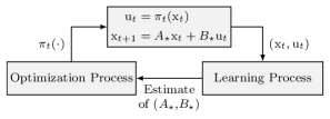
Figure 1: Schematic representation of the stability-certified on-policy LQR setup.

2.2 Preliminaries: Model-based Gradient Method for LQR

Next, we recall the key ingredients for devising a model-based gradient method to address problem (1).

2.2.1 Model-based reduced problem formulation

First of all, we recall an equivalent (unconstrained) formulation of problem (1) that explicitly imposes the linear feedback structure to the optimal input and is amenable for gradient-based algorithmic solutions. Problem (1) is rewritten by substituting in the dynamics and in the cost function the input in linear feedback form $\mathrm{u}_{t}=K\mathrm{\mathrm{x}}_{t}$, where $K\in\mathbb{R}^{{m}\times{n}}$ is to be computed. First of all, given any gain $K$, the original (open-loop) dynamics (1b) admits the closed-loop formulation $\mathrm{\mathrm{x}}_{{t+1}}=({A}_{\star}+{B}_{\star}K)\mathrm{\mathrm{x}}_{t}$. So that, for all $t\geq 0$, the state is uniquely determined as

$$\mathrm{\mathrm{x}}_{t}=({A}_{\star}+{B}_{\star}K)^{t}\mathrm{x}_{0},\qquad\mathrm{x}_{0}\sim\mathcal{X}_{0}.$$ (3)

Hence, leveraging on (3), assuming that $\mathcal{X}_{0}$ is a uniform distribution on the unit sphere, and taking the expected value on the initial condition, problem (1) can be rewritten as

$$\min_{K\in\mathcal{K}}\> \>J(K,\theta^{\star}),$$ (4)

where $\theta^{\star}$ is defined in (2), while, given the set of stabilizing gains $\mathcal{K}:=\{K\in\mathbb{R}^{m\times n}\mid{A}_{\star}+{B}_{\star}K\text{ is Schur}\}\subseteq\mathbb{R}^{m\times n}$, we introduced $J:\mathcal{K}\times\mathbb{R}^{(n+m)\times n}\to\mathbb{R}$ defined as

$$J(K,\theta^{\star})=\tfrac{1}{2}\operatorname{Tr}\left(\sum_{t=0}^{\infty}({A}_{\star}+{B}_{\star}K)^{t,\top}(Q+K^{\top}RK)({A}_{\star}+{B}_{\star}K)^{t}\right).$$ (5)

This formulation highlights that (i) the overall problem actually depends on the gain $K$ only, and, (ii) the optimal gain $K^{\star}$ does not depend on the initial condition $\mathrm{x}_{0}$.

2.2.2 Model-based gradient method for problem (4)

The set of stabilizing gains $\mathcal{K}$ is open [46, Lemma IV.3] and connected [46, Lemma IV.6], therefore, if the pair $({A}_{\star},{B}_{\star})$ were known, the gradient descent method could be used to solve problem (4) (see, e.g., [30]). Namely, at each iteration $t\in\mathbb{N}$, an estimate $K_{t}$ of $K^{\star}$ is maintained and iteratively updated according to

$$K_{{t+1}}=K_{t}-\gamma G(K_{t},\theta^{\star}),$$ (6)

where $\gamma>0$ is the stepsize, while $G:\mathbb{R}^{m\times n}\times\mathbb{R}^{(n+m)\times n}\to\mathbb{R}^{m\times n}$ is the gradient of $J$ with respect to $K$ evaluated at $(K_{t},\theta^{\star})$, when $\mathbb{R}^{m\times n}$ is equipped with the Frobenius inner product. It is possible to show that, by initializing $K_{0}\in\mathcal{K}$ and selecting a proper stepsize $\gamma$, the optimal gain $K^{\star}$ is an exponentially stable equilibrium of the dynamical system (6), see [30, Theorem 4.6]. The procedure to compute and evaluate the gradient $G(K_{t},\theta^{\star})$ reads as follows:

1. solve for $W^{c}_{t}\in\mathbb{R}^{n\times n}$ and $P_{t}\in\mathbb{R}^{n\times n}$ the equations

   $$\begin{split}&({A}_{\star}+{B}_{\star}K_{t})W^{c}_{t}({A}_{\star}+{B}_{\star}K_{t})^{\top}-W^{c}_{t}=-I_{n}\\ &({A}_{\star}+{B}_{\star}K_{t})^{\top}P_{t}({A}_{\star}+{B}_{\star}K_{t})-P_{t}=-(Q+{K_{t}}^{\top}RK_{t})\end{split}$$

2. compute the gradient $G(K_{t},\theta^{\star})$ as

   $$G(K_{t},\theta^{\star})\!=\!\left(RK_{t}+{B}_{\star}^{\top}P_{t}({A}_{\star}+{B}_{\star}K_{t})\right)W^{c}_{t}.$$ (7)

Notice that our goal is to address the problem setup described in Section 2.1 without knowing $\theta^{\star}$. Hence, in our framework, it is not possible to implement update (6).

3 On-policy LQR for Unknown Systems: Concurrent Learning and Optimization

In this section, we formally present Relearn LQR, a concurrent learning and optimization algorithm developed to solve the stability-certified on-policy LQR setup described in Section 2.1. The proposed on-policy strategy feeds the real system at each iteration $t$ with the current feedback input including also an exogenous dithering signal $\mathrm{w}_{t}$. Then, a new sample data from the system is collected and used to progressively improve the estimates $({A}_{t},{B}_{t})$ of the unknown $({A}_{\star},{B}_{\star})$ via a learning process inspired by Recursive Least Squares (RLS). In turn, $({A}_{t},{B}_{t})$ is used to refine the feedback gain $K_{t}$ according to the gradient method, and the system is actuated in closed-loop. Figure 2 shows the overall scheme.

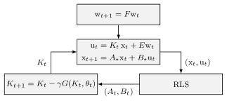
Figure 2: Representation of the concurrent learning and optimization scheme implemented by Relearn LQR.

The overall Relearn LQR strategy is reported in Algorithm 1 where, for notational convenience, we denote as $\theta_{t}\in\mathbb{R}^{(n+m)\times n}$ the estimate of $\theta^{\star}$ at iteration $t\in\mathbb{N}$. Consistently, ${A}_{t}\in\mathbb{R}^{n\times n}$ and ${B}_{t}\in\mathbb{R}^{n\times m}$ are the corresponding estimates of $A$ and $B$. Moreover, $H_{t}\in\mathbb{R}^{(n+m)\times(n+m)}$ and $S_{t}\in\mathbb{R}^{(n+m)\times n}$ denote two additional states of the learning process, $\lambda\in(0,1)$ is a forgetting factor, while $\gamma$ is the stepsize as in (6). Finally, in order to prescribe the initialization $K_{0}$, we introduce the set $\mathcal{K}_{b}(K^{\star})\subset\mathcal{K}$ defined as the largest ball centered in $K^{\star}$ and contained in $\mathcal{K}$.

Initialization: $\mathrm{x}_{0}\in\mathbb{R}^{n}$, $H_{0}\in\mathbb{R}^{(n+m)\times(n+m)}$, $S_{0}\in\mathbb{R}^{(n+m)\times n}$, $\theta_{0}\!\in\!\mathbb{R}^{(n+m)\times n},K_{0}\!\in\!\mathbb{R}^{m\times n}$ and $\mathrm{w}_{0}\!\in\!\mathbb{R}^{n_{\mathrm{w}}}$.

for $t=0,1,2\ldots$ do

     Data collection: generate

$$\mathrm{w}_{{t+1}} =F\mathrm{w}_{t}$$

$$\mathrm{d}_{t} =E\mathrm{w}_{t}$$

     and actuate

$$\mathrm{u}_{t} =K_{t}\mathrm{\mathrm{x}}_{t}+\mathrm{d}_{t}$$

$$\mathrm{\mathrm{x}}_{{t+1}} ={A}_{\star}\mathrm{\mathrm{x}}_{t}+{B}_{\star}\mathrm{u}_{t}$$

$$\mathrm{y}_{t} =\mathrm{\mathrm{x}}_{{t+1}}^{\top}$$

     Learning process: compute

$$H_{{t+1}} =\lambda H_{t}+\begin{bmatrix}\mathrm{\mathrm{x}}_{t}\\ \mathrm{u}_{t}\end{bmatrix}\begin{bmatrix}\mathrm{\mathrm{x}}_{t}\\ \mathrm{u}_{t}\end{bmatrix}^{\top}$$ (8a)

$$S_{{t+1}} =\lambda S_{t}+\begin{bmatrix}\mathrm{\mathrm{x}}_{t}\\ \mathrm{u}_{t}\end{bmatrix}\mathrm{y}_{t}$$ (8b)

$$\theta_{{t+1}} =\theta_{t}-\gamma H_{t}^{\dagger}\left(H_{t}\theta_{t}-S_{t}\right).$$ (8c)

     Optimization process: update

$$K_{{t+1}}=K_{t}-\gamma G(K_{t},\theta_{t}).$$ (9)

Algorithm 1 Relearn LQR

Next, we detail the main steps of the proposed algorithm.

Data collection

Data from the controlled system (1b) are recast in an identification-oriented form described by

$$\underbrace{\mathrm{\mathrm{x}}_{{t+1}}^{\top}}_{\displaystyle\mathrm{y}_{t}}=\underbrace{\begin{bmatrix}\mathrm{\mathrm{x}}_{t}^{\top}&\mathrm{u}_{t}^{\top}\end{bmatrix}}_{\displaystyle C(\mathrm{\mathrm{x}}_{t},\mathrm{u}_{t})^{\top}}\underbrace{\begin{bmatrix}{A}_{\star}^{\top}\\ {B}_{\star}^{\top}\end{bmatrix}}_{\displaystyle\theta^{\star}}.$$ (10)

Learning process

The adopted learning strategy to compute an estimate of $\theta^{\star}$ relies on the interpretation of the least squares problem as an online optimization. Specifically, with the measurements (10) at hand, we consider, at each $t\in\mathbb{N}$, the online optimization problem

$$\min_{\theta\in\mathbb{R}^{(n+m)\times n}}\tfrac{1}{2}\sum_{\tau=0}^{t}\lambda^{t-\tau}\left\|C(\mathrm{x}_{\tau},\mathrm{u}_{\tau})^{\top}\theta-\mathrm{y}_{\tau}\right\|^{2}.$$ (11)

We aim to solve (11) through an iterative algorithm that progressively refines a solution estimate $\theta_{t}\in\mathbb{R}^{(n+m)\times n}$. In particular, the estimate $\theta_{t}$ can be updated through a “scaled” gradient method with Newton’s like scaling matrix, which reads as

$$\theta_{{t+1}}=\theta_{t}-\gamma \left(\sum_{\tau=0}^{t}\lambda^{t-\tau}\mathcal{H}(\mathrm{x}_{\tau},\mathrm{u}_{\tau})\right)^{\dagger}\times\left(\sum_{\tau=0}^{t}\lambda^{t-\tau}\left(\mathcal{H}(\mathrm{x}_{\tau},\mathrm{u}_{\tau})\theta_{t}-\mathcal{S}(\mathrm{x}_{\tau},\mathrm{u}_{\tau},\mathrm{y}_{\tau})\right)\right),$$

where $\mathcal{H}:\mathbb{R}^{n}\times\mathbb{R}^{m}\to\mathbb{R}^{(n+m)\times(n+m)}$ and $\mathcal{S}:\mathbb{R}^{n}\times\mathbb{R}^{m}\times\mathbb{R}^{n}\to\mathbb{R}^{(n+m)\times n}$ reads as

$$\mathcal{H}(\mathrm{x}_{\tau},\mathrm{u}_{\tau}) :=C(\mathrm{x}_{\tau},\mathrm{u}_{\tau})C(\mathrm{x}_{\tau},\mathrm{u}_{\tau})^{\top}$$

$$\mathcal{S}(\mathrm{x}_{\tau},\mathrm{u}_{\tau},\mathrm{y}_{\tau}) :=C(\mathrm{x}_{\tau},\mathrm{u}_{\tau})\mathrm{y}_{\tau}.$$

To overcome the issue of storing the whole history of $\mathcal{H}(\cdot,\cdot)$ and $\mathcal{S}(\cdot,\cdot,\cdot)$, we iteratively keep track of them through the matrix states $H_{t}\in\mathbb{R}^{(n+m)\times(n+m)}$ and $S_{t}\in\mathbb{R}^{(n+m)\times n}$ giving rise to (8).

Optimization process

The estimate $\theta_{t}$ is concurrently exploited in the update of the feedback gain $K_{t}$, replacing the unavailable $\theta^{\star}$ into (6) giving rise to (9).

To ensure sufficiently informative data, we equip our feedback policy with an additive dithering signal $\mathrm{d}_{t}\in\mathbb{R}^{m}$. Namely, we implement

$$\mathrm{u}_{t}=K_{t}\mathrm{\mathrm{x}}_{t}+\mathrm{d}_{t},$$ (12)

where $\mathrm{d}_{t}$ is the output of an exogenous system evolving according to a marginally stable linear discrete-time oscillator dynamics (see, e.g., [47]) described by

$$\mathrm{w}_{{t+1}} =F\mathrm{w}_{t}$$ (13a)

$$\mathrm{d}_{t} =E\mathrm{w}_{t},$$ (13b)

where $\mathrm{w}_{t}\in\mathbb{R}^{n_{\mathrm{w}}}$, with $n_{\mathrm{w}}\geq n+m$, is the state of the exogenous system having $F\in\mathbb{R}^{n_{\mathrm{w}}\times n_{\mathrm{w}}}$ and $E\in\mathbb{R}^{n_{\mathrm{w}}}$ as state and output matrix, respectively. The matrix $F$ is a degree of freedom to properly shape the oscillation frequency of $\mathrm{w}_{t}$. The following assumption formalizes the requirements for the design of system (13).

Assumption 3.1 (Persistency of Excitation)

The signals $\mathrm{w}_{t}$ and $\mathrm{d}_{t}$ are persistently exciting and sufficiently rich of order $({n}+1)$, respectively, i.e., there exist $\alpha_{1},\alpha_{2},t_{\mathrm{w}},\mathbf{t}_{\mathrm{d}}>0$ such that, if $\mathrm{w}_{0}\neq 0_{n_{\mathrm{w}}}$, then

$$\alpha_{1}I_{n_{\mathrm{w}}}\leq\sum_{\tau=\bar{t}+1}^{\bar{t}+t_{\mathrm{w}}}\mathrm{w}_{\tau}\mathrm{w}_{\tau}^{\top}\leq\alpha_{2}I_{n_{\mathrm{w}}},\quad\textnormal{ for all $\bar{t}\in\mathbb{N}$ }$$ (14a)

$$\operatorname{rank}\left(\begin{bmatrix}\mathrm{d}_{0}&\mathrm{d}_{1}&\ldots&\mathrm{d}_{\mathbf{t}_{\mathrm{d}}-n-1}\\ \mathrm{d}_{1}&\mathrm{d}_{2}&&\mathrm{d}_{\mathbf{t}_{\mathrm{d}}-n}\\ \vdots&\vdots&\ddots&\vdots\\ \mathrm{d}_{n}&\mathrm{d}_{n+1}&\ldots&\mathrm{d}_{\mathbf{t}_{\mathrm{d}}-1}\end{bmatrix}\right)=m(n+1).$$ (14b)

Moreover, the eigenvalues of $F$ lie on the unit disk. $\blacksquare$

We point out that recent references, see, e.g., [48, 14], refer to the property (14b) as persistency of excitation of order $(n+1)$, while we used the equivalent definition of sufficient richness of order $(n+1)$, see, e.g., [49].

The overall closed-loop dynamics resulting from Algorithm 1 can be rewritten as

$$\mathrm{w}_{{t+1}} =F\mathrm{w}_{t}$$ (15a)

$$\mathrm{\mathrm{x}}_{{t+1}} =({A}_{\star}+{B}_{\star}K_{t})\mathrm{\mathrm{x}}_{t}+{B}_{\star}E\mathrm{w}_{t}$$ (15b)

$$H_{{t+1}} =\lambda H_{t}+\begin{bmatrix}\mathrm{\mathrm{x}}_{t}\\ K_{t}\mathrm{\mathrm{x}}_{t}+E\mathrm{w}_{t}\end{bmatrix}\begin{bmatrix}\mathrm{\mathrm{x}}_{t}\\ K_{t}\mathrm{\mathrm{x}}_{t}\!+\!E\mathrm{w}_{t}\end{bmatrix}^{\top}$$ (15c)

$$S_{{t+1}} =\lambda S_{t}+\begin{bmatrix}\mathrm{\mathrm{x}}_{t}\\ K_{t}\mathrm{\mathrm{x}}_{t}\!+\!E\mathrm{w}_{t}\end{bmatrix}\begin{bmatrix}\mathrm{\mathrm{x}}_{t}\\ K_{t}\mathrm{\mathrm{x}}_{t}\!+\!E\mathrm{w}_{t}\end{bmatrix}^{\top}\theta^{\star}$$ (15d)

$$\theta_{{t+1}} =\theta_{t}-\gamma H_{t}^{\dagger}\left(H_{t}\theta_{t}-S_{t}\right)$$ (15e)

$$K_{{t+1}} =K_{t}-\gamma G(K_{t},\theta_{t}),$$ (15f)

in which we have used the explicit expressions for $\mathrm{y}_{t}$ (cf. (10)) and $\mathrm{u}_{t}$ (cf. (12)). Next, we provide the main result of the paper, i.e., the convergence properties of system (15). For the sake of compactness, we introduce $\mathcal{V}:=(\mathbb{R}^{n_{\mathrm{w}}}\setminus\{0\})\times\mathbb{R}^{n}\times\mathbb{R}^{(n+m)\times(n+m)}\times\mathbb{R}^{(n+m)\times n}\times\Theta_{b}\times\mathcal{K}_{b}(K^{\star})$ and the operators $\mathrm{v}_{H}:\mathbb{R}^{(n+m)^{2}\times n_{\mathrm{w}}^{2}}\times\mathbb{R}^{n}_{\mathrm{w}}\to\mathbb{R}^{(n+m)\times(n+m)}$ and $\mathrm{v}_{S}:\mathbb{R}^{(n+m)m\times n_{\mathrm{w}}^{2}}\times\mathbb{R}^{n}_{\mathrm{w}}\to\mathbb{R}^{(n+m)\times n}$ defined as

$$\mathrm{v}_{H}(\Pi_{H},\mathrm{w}) :=\mathtt{unvec}\left(\Pi_{H}\mathtt{vec}\left(\mathrm{w}\mathrm{w}^{\top}\right)\right)$$

$$\mathrm{v}_{S}(\Pi_{S},\mathrm{w}) :=\mathtt{unvec}\left(\Pi_{S}\mathtt{vec}\left(\mathrm{w}\mathrm{w}^{\top}\right)\right),$$

where $\Pi_{H}\in\mathbb{R}^{(n+m)^{2}\times n_{\mathrm{w}}^{2}}$, $\Pi_{S}\in\mathbb{R}^{(n+m)m\times n_{\mathrm{w}}^{2}}$.

Theorem 3.2

Consider system (15) and let Assumptions 2.1 and 3.1 hold. Then, for each initial condition $(\mathrm{w}_{0},\mathrm{x}_{0},H_{0},S_{0},\theta_{0},K_{0})\in\mathcal{V}$ such that $A_{0}+B_{0}K_{0}$ is Schur, there exist $\Pi_{\mathrm{x}}\in\mathbb{R}^{n\times n_{\mathrm{w}}}$, $\Pi_{H}\in\mathbb{R}^{(n+m)^{2}\times n_{\mathrm{w}}^{2}}$, $\Pi_{S}\in\mathbb{R}^{(n+m)m\times n_{\mathrm{w}}^{2}}$, $a_{1},a_{2},a_{3},a_{4},a_{5},a_{6},a_{7},a_{8},\bar{\gamma}>0$ such that, it holds

$$\left\|\mathrm{\mathrm{x}}_{t}-\Pi_{\mathrm{x}}\mathrm{w}_{t}\right\|\leq a_{1}\left\|\mathrm{x}_{0}-\Pi_{\mathrm{x}}\mathrm{w}_{0}\right\|\exp(-a_{2}t)$$ (16a)

$$\left\|H_{t}\!-\!\mathrm{v}_{H}(\Pi_{H},\!\mathrm{w}_{t})\right\|\leq a_{3}\!\left\|H_{0}\!-\!\mathrm{v}_{H}(\Pi_{H},\!\mathrm{w}_{0})\right\|\!\exp(-a_{4}t)$$ (16b)

$$\left\|S_{t}\!-\!\mathrm{v}_{S}(\Pi_{S},\mathrm{w}_{t})\right\|\leq a_{5}\!\left\|S_{0}\!-\!\mathrm{v}_{S}(\Pi_{S},\mathrm{w}_{0})\right\|\!\exp(-a_{6}t)$$ (16c)

$$\left\|\begin{bmatrix}\theta_{t}-\theta^{\star}\\ K_{t}-K^{\star}\end{bmatrix}\right\|\leq a_{7}\left\|\begin{bmatrix}\theta_{0}-\theta^{\star}\\ K_{0}-K^{\star}\end{bmatrix}\right\|\exp(-a_{8}t),$$ (16d)

for all $\gamma\in(0,\bar{\gamma})$. $\blacksquare$

The proof of Theorem 3.2 is provided in Section 4.3.

The result (16a) of Theorem 3.2 ensures that the origin is an exponentially practically stable equilibrium for (15b). Indeed Theorem 3.2 allows us to choose the initial condition of the exogenous system $\mathrm{w}_{0}$ so that $\mathrm{\mathrm{x}}_{t}$ exponentially converges into the ball $\mathcal{B}_{\rho}(0_{n})$ for any desired radius $\rho>0$. More in details, since $\mathrm{w}_{t}$ evolves according to a marginally stable oscillating dynamics (cf. Assumption 3.1), it holds $\left\|\mathrm{w}_{t}\right\|=\left\|\mathrm{w}_{0}\right\|$ for all $t\in\mathbb{N}$. Thus, in order to make $\mathcal{B}_{\rho}(0_{n})$ attractive for the trajectories of (15b), it is sufficient to choose $\mathrm{w}_{0}$ such that

$$\left\|\mathrm{w}_{0}\right\|\leq\dfrac{\rho}{\left\|\Pi_{\mathrm{x}}\right\|}.$$

Furthermore, the result (16d) ensures that $(K^{\star},\theta^{\star})$ is exponentially stable for (15e) and (15f). Hence, we asymptotically (i) reconstruct the unknown system matrices $({A}_{\star},{B}_{\star})$ and (ii) compute the optimal gain matrix $K^{\star}$.

4 Stability Analysis

In this section, we perform the stability analysis of the closed-loop dynamics arising from Algorithm 1. First, we write the algorithm dynamics with respect to suitable error coordinates. Second, we resort to the averaging theory to prove the exponential stability of the origin for the averaged system associated to the error dynamics. This result is then exploited to prove Theorem 3.2.

4.1 Closed-Loop Dynamics in Error Coordinates

As a preliminary step, system (15) is expressed into suitably defined error coordinates. First, we consider vectorized versions of the matrix updates in (15c)-(15d). To this end, let the new coordinates $H^{\text{vc}}\in\mathbb{R}^{(n+m)^{2}}$ and $S^{\text{vc}}\in\mathbb{R}^{(n+m)n}$ be defined as

$$\begin{cases}H_{t}\\ S_{t}\\ \end{cases}\longmapsto\begin{cases}H^{\text{vc}}_{t}:=\mathtt{vec}\left(H_{t}\right)\\ S^{\text{vc}}_{t}:=\mathtt{vec}\left(S_{t}\right).\end{cases}$$ (17)

Therefore, (15c)-(15d) can be recast as

$$H^{\text{vc}}_{t+1}\! =\!\lambda H^{\text{vc}}_{t}\!+\!\mathtt{vec}\left(\!\begin{bmatrix}\mathrm{\mathrm{x}}_{t}\\ K_{t}\mathrm{\mathrm{x}}_{t}\!+\!E\mathrm{w}_{t}\end{bmatrix}\!\!\!\begin{bmatrix}\mathrm{\mathrm{x}}_{t}\\ K_{t}\mathrm{\mathrm{x}}_{t}\!+\!E\mathrm{w}_{t}\end{bmatrix}^{\top}\!\right)$$ (18a)

$$S^{\text{vc}}_{t+1}\! =\!\lambda S^{\text{vc}}_{t}\!+\!\mathtt{vec}\left(\!\begin{bmatrix}\mathrm{\mathrm{x}}_{t}\\ K_{t}\mathrm{\mathrm{x}}_{t}\!+\!E\mathrm{w}_{t}\end{bmatrix}\!\!\!\begin{bmatrix}\mathrm{\mathrm{x}}_{t}\\ K_{t}\mathrm{\mathrm{x}}_{t}\!+\!E\mathrm{w}_{t}\end{bmatrix}^{\top}\!\!\!\theta^{\star}\!\right)\!\!.$$ (18b)

Next, we will inspect (18) together with (15b) to provide the steady-state locus (see, e.g., [50, Ch. 12] for a formal definition) when the system is fed with the signal $\mathrm{w}_{t}$, which evolves according to (15a). To this end, set $n_{\chi}:=n+(n+m)^{2}+(n+m)n$ and let $\chi\in\mathbb{R}^{n_{\chi}}$ be defined as

$$\chi:=\begin{bmatrix}\mathrm{x}^{\top}&(H^{\text{vc}})^{\top}&(S^{\text{vc}})^{\top}\end{bmatrix}^{\top}.$$

Then, using (18), the dynamics in (15a)-(15d) can be compactly expressed in the new coordinates as

$$\mathrm{w}_{{t+1}} =F\mathrm{w}_{t}$$ (19a)

$$\chi_{t+1} =\mathcal{A}_{K}(K_{t})\chi_{t}+\phi(\chi_{t},K_{t},\mathrm{w}_{t})$$ (19b)

where we introduced $\mathcal{A}_{K}:\mathbb{R}^{m\times n}\to\mathbb{R}^{n_{\chi}\times n_{\chi}}$ and $\phi:\mathbb{R}^{n_{\chi}}\times\mathbb{R}^{m\times n}\times\mathbb{R}^{n_{\mathrm{w}}}\to\mathbb{R}^{n_{\chi}}$ be defined as

$$\mathcal{A}_{K}(K) :=\begin{bmatrix}{A}_{\star}+{B}_{\star}K&0&0\\ 0&\lambda I&0\\ 0&0&\lambda I\end{bmatrix}$$ (20a)

$$\phi(\chi,K,\mathrm{w}) :=\begin{bmatrix}{B}_{\star}E\mathrm{w}\\ \mathtt{vec}\left(\begin{bmatrix}\mathrm{x}\\ K\mathrm{x}\!+\!E\mathrm{w}\end{bmatrix}\begin{bmatrix}\mathrm{x}\\ K\mathrm{x}\!+\!E\mathrm{w}\end{bmatrix}^{\top}\right)\\ \mathtt{vec}\left(\begin{bmatrix}\mathrm{x}\\ K\mathrm{x}\!+\!E\mathrm{w}\end{bmatrix}\begin{bmatrix}\mathrm{x}\\ K\mathrm{x}\!+\!E\mathrm{w}\end{bmatrix}^{\top}\theta^{\star}\right)\end{bmatrix}.$$ (20b)

Notice that to keep the notation light, we use a hybrid notation with $\chi$ on the left-hand side and its (unvectorized) components $(\mathrm{x},H,S)$ on the right-hand side.

System (19) together with the exosystem (15a) is a cascade whose steady-state locus can be characterized by the nonlinear map $\chi^{{\textnormal{ss}}}:\mathbb{R}^{n_{\mathrm{w}}}\to\mathbb{R}^{n_{\chi}}$ defined as

$$\chi^{{\textnormal{ss}}}(\mathrm{w}):=\begin{bmatrix}\Pi_{\mathrm{x}}\mathrm{w}\\ \Pi_{H}\mathtt{vec}\left(\mathrm{w}\mathrm{w}^{\top}\right)\\ \Pi_{S}\mathtt{vec}\left(\mathrm{w}\mathrm{w}^{\top}\right)\end{bmatrix},$$ (21)

where $\Pi_{\mathrm{x}}$, $\Pi_{H}$, and $\Pi_{S}$ are the same as in Theorem 3.2 (see (B.2) and (B.6) in Appendix B for their explicit definition). Formally, the following lemma holds true.

Lemma 4.1

Let the assumptions of Theorem 3.2 hold true. Consider the map $\chi^{{\textnormal{ss}}}$ defined in (21), the feedback gain $K^{\star}$ solving (1), the matrix $F$ as in (13), and the functions $\mathcal{A}_{K}$ and $\phi$ defined in (20). Then, it holds

$$\chi^{{\textnormal{ss}}}(F\mathrm{w})=\mathcal{A}_{K}(K^{\star})\chi^{{\textnormal{ss}}}(\mathrm{w})+\phi(\chi^{{\textnormal{ss}}}(\mathrm{w}),K^{\star},\mathrm{w}),$$ (22)

for all $\mathrm{w}\in\mathbb{R}^{n_{\mathrm{w}}}$. Moreover, it holds

$$({\theta^{\star}}^{\top}\otimes I_{n+m})\Pi_{H}=\Pi_{S}.$$ (23)

$\blacksquare$

The proof of Lemma 4.1 is provided in Appendix B.

Lemma 4.1 ensures that $\operatorname{col}(\chi^{{\textnormal{ss}}}(\mathrm{w}),\theta^{\star},K^{\star})$ is the steady-state locus of the overall closed-loop system (15). In this regard, we also included condition (23) since it allows us to show that $\theta^{\star}$ is an equilibrium of update (15e) restricted to the case in which $H_{t}$ and $S_{t}$ lie in the steady-state locus. Indeed, when $\chi_{t}=\chi^{{\textnormal{ss}}}(\mathrm{w}_{t})$, the update (15e) reduces to

$$\theta_{{t+1}}\Big{|}_{\chi_{t}=\chi^{{\textnormal{ss}}}(\mathrm{w}_{t})} =\theta_{t}-\gamma\left(H_{t}\theta_{t}-S_{t}\right)\Big{|}_{\chi_{t}=\chi^{{\textnormal{ss}}}(\mathrm{w}_{t})}$$

$$=\theta_{t}-\gamma\mathrm{v}_{S}(\Pi_{S},\mathrm{w}_{t})\theta_{t}$$

$$=\theta_{t}-\gamma\mathtt{unvec}\left(\left({\theta^{\star}}^{\top}\otimes I_{n+m}\right)\Pi_{H}\mathtt{vec}\left(\mathrm{w}_{t}\mathrm{w}_{t}^{\top}\right)\right)$$

$$\stackrel{{\scriptstyle(a)}}{{=}}\theta_{t}-\gamma\mathrm{v}_{H}(\Pi_{H},\mathrm{w}_{t})\left(\theta_{t}-\theta^{\star}\right),$$

where in $(a)$ we used a property of the vectorization operator. As for the equilibrium of (15f) when the other states lie on the steady-state locus, it turns out to be $K^{\star}$ since $G(K^{\star},\theta^{\star})=0$.

Before proceeding, let us collect also the remaining states in (15) in $\mathrm{z}\in\mathbb{R}^{n_{\mathrm{z}}}$, with $n_{\mathrm{z}}:=(n+2m)\times n$, defined as

$$\mathrm{z}:=\begin{bmatrix}\theta^{\top}&K^{\top}\end{bmatrix}^{\top}.$$

In order to prove Theorem 3.2, we need to show the convergence of $\chi$ and $\mathrm{z}$ toward $\chi^{{\textnormal{ss}}}(\mathrm{w})$ and $\operatorname{col}(\theta^{\star},K^{\star})$, respectively. Therefore, with Lemma 4.1 at hand, let us introduce error coordinates $\tilde{\chi}\in\mathbb{R}^{n_{\chi}}$ and $\tilde{\mathrm{z}}\in\mathbb{R}^{n_{\mathrm{z}}}$ given by the following change of coordinates

$$\begin{cases}\mathrm{w}\\ \chi\\ \mathrm{z}\end{cases}\longmapsto\begin{cases}\mathrm{w}\\ \tilde{\chi}:=\begin{bmatrix}I&0&0\\ 0&\gamma I&0\\ 0&0&\gamma I\end{bmatrix}\left(\chi-\chi^{{\textnormal{ss}}}(\mathrm{w})\right)\\ \tilde{\mathrm{z}}:=\mathrm{z}-\begin{bmatrix}\theta^{\star}\\ K^{\star}\end{bmatrix}.\end{cases}$$ (24)

For notational convenience, we will sometimes refer to the components of $\tilde{\mathrm{z}}$ as $\operatorname{col}(\tilde{\theta},\tilde{K})$. Finally, the closed-loop dynamics (15) in the new coordinates (24) reads as

$$\tilde{\chi}_{t+1} =\mathcal{A}(\tilde{\mathrm{z}}_{t})\tilde{\chi}_{t}+h(\tilde{\mathrm{z}}_{t},t)+\gamma g(\tilde{\chi}_{t},\tilde{\mathrm{z}}_{t},t)$$ (25a)

$$\tilde{\mathrm{z}}_{t+1} =\tilde{\mathrm{z}}_{t}+\gamma f(\tilde{\chi}_{t},\tilde{\mathrm{z}}_{t},t),$$ (25b)

where $\mathcal{A}(\tilde{\mathrm{z}}):=\mathcal{A}_{K}(\tilde{K}+K^{\star})$ and we introduced $h:\mathbb{R}^{n_{\mathrm{z}}}\times\mathbb{N}\to\mathbb{R}^{n_{\mathrm{z}}}$, $g:\mathbb{R}^{n_{\chi}}\times\mathbb{R}^{n_{\mathrm{z}}}\times\mathbb{N}\to\mathbb{R}^{n_{\chi}}$, and $f:\mathbb{R}^{n_{\chi}}\times\mathbb{R}^{n_{\mathrm{z}}}\times\mathbb{N}\to\mathbb{R}^{n_{\mathrm{z}}}$ defined respectively as

$$h(\tilde{\mathrm{z}},t) :=\begin{bmatrix}{B}_{\star}\tilde{K}\Pi_{\mathrm{x}}\mathrm{w}_{t}\\ 0\\ 0\end{bmatrix}$$ (26a)

$$g(\tilde{\chi},\tilde{\mathrm{z}},t) :=\begin{bmatrix}0\\ \gamma\phi(\tilde{\mathrm{x}}+\Pi_{\mathrm{x}}\mathrm{w}_{t},\tilde{K}+K^{\star},\mathrm{w}_{t})\end{bmatrix}$$ (26b)

$$f(\tilde{\chi},\tilde{\mathrm{z}},t) :=-\begin{bmatrix}(\tilde{H}+H^{{\textnormal{ss}}}_{t})^{\dagger}\left((\tilde{H}+H^{{\textnormal{ss}}}_{t})\tilde{\theta}+(\tilde{H}-\tilde{S})\theta^{\star}\right)\\ G(\tilde{K}+K^{\star},\tilde{\theta}+\theta^{\star})\end{bmatrix}.$$ (26c)

Notice that for the sake of readability, in (26) we used the shorthands $\tilde{\chi}:=\operatorname{col}(\tilde{\mathrm{x}},\tilde{H},\tilde{S})$ and $\tilde{\mathrm{z}}=\operatorname{col}(\tilde{\theta},\tilde{K})$, we defined $H^{{\textnormal{ss}}}_{t}\in\mathbb{R}^{(n+m)\times(n+m)}$ as

$$H^{{\textnormal{ss}}}_{t} :=\mathrm{v}_{H}(\Pi_{H},\mathrm{w}_{t}),$$ (27)

which represents the steady-state value of the state $H_{t}$ and we introduced the error coordinates $\tilde{H}\in\mathbb{R}^{(n+m)\times(n+m)}$ and $\tilde{S}\in\mathbb{R}^{(n+m)\times n}$, as

$$\tilde{H} :=\mathtt{unvec}\left(H^{\text{vc}}-H^{{\textnormal{ss}}}_{t}\right)$$ (28a)

$$\tilde{S} :=\mathtt{unvec}\left(S^{\text{vc}}-\Pi_{S}\mathtt{vec}\left(\mathrm{w}_{t}\mathrm{w}_{t}^{\top}\right)\right).$$ (28b)

Some remarks are in order. We point out that with this transformation we obtained a dynamical system with two-time scales as the one described in Appendix A (cf. system (A.1)). As customary in the context of singularly perturbed systems, we distinguish between (i) the fast dynamics (25a) with state $\tilde{\chi}$, and (ii) the slow one (25b) with state $\tilde{\mathrm{z}}$. Figure 3 shows the mentioned interconnected structure of system (25).

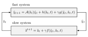
Figure 3: Block diagram describing system (25).

It is also worth noting that, in this reformulation, the effect of the exogenous/dithering signal $\mathrm{w}_{t}$ has been embedded in the time dependency of $h$, $g$, and $f$. As for the equilibrium manifold, we observe that it holds

$$h(0,t)=0,\qquad g(0,0,t)=0,\qquad f(0,0,t)=0,$$ (29)

for all $t\in\mathbb{N}$. Finally, the matrix $\mathcal{A}(\tilde{\mathrm{z}})$ is Schur for all $\tilde{K}\in\mathbb{R}^{m\times n}$ such that $(\tilde{K}+K^{\star})\in\mathcal{K}$.

4.2 Averaged System Analysis

Next, we carry out the stability analysis of the time-varying system (25) by leveraging on the averaging and singular perturbations theories (cf. Appendix A for further details). Indeed, since system (25) enjoys a two-time-scale structure (cf. the generic system (A.1) in Appendix A), we can study (25) by only investigating an auxiliary system typically termed as the averaged system. The latter is obtained by considering the slow dynamics (25b) in which (i) the fast state is frozen to its equilibrium, i.e., with $\tilde{\chi}_{t}=0$ for all $t\geq 0$, and (ii) the vector field describing the dynamics is averaged with respect to time.

The following result is instrumental to properly write the averaged system.

Lemma 4.2

Let the assumptions of Theorem 3.2 hold true. Consider $f$ defined in (26c). Then, it holds

$$\lim_{T\to\infty}\frac{1}{T}\sum_{\tau=\bar{t}+1}^{\bar{t}+T}f(0,\tilde{\mathrm{z}},\tau)=\!-\!\begin{bmatrix}\tilde{\theta}\\ G(\tilde{K}\!+\!K^{\star},\tilde{\theta}\!+\!\theta^{\star})\end{bmatrix}$$ (30)

uniformly in $\bar{t}\in\mathbb{N}$ and for all $\tilde{\mathrm{z}}=\operatorname{col}(\tilde{\theta},\tilde{K})\in\mathbb{R}^{n_{\mathrm{z}}}$. $\blacksquare$

The proof of Lemma 4.2 is given in Appendix C.

Lemma 4.2 provides a suitable approximation of the dynamics of $\tilde{\mathrm{z}}$ in (25b) when (i) the convergence of the fast state $\tilde{\chi}$ to its equilibrium has already occurred and (ii) by averaging over time $t$ the vector field $f(0,\tilde{\mathrm{z}},t)$. Specifically, under this approximation, Lemma 4.2 ensures that the two components of the driving term of the dynamics of $\tilde{\mathrm{z}}$ are given by (i) a proportional term $-\gamma\tilde{\theta}$ and (ii) an approximate version of the correct gradient $G(\tilde{K}+K^{\star},\theta^{\star})$. Next, we will leverage averaging theory to prove the stability of the origin for system (25).

Once the averaged vector field has been characterized in Lemma 4.2, we can introduce $f^{\textsc{av}}:\mathbb{R}^{n_{\mathrm{z}}}\to\mathbb{R}^{n_{\mathrm{z}}}$ given by

$$f^{\textsc{av}}(\tilde{\mathrm{z}})\!:=\!\lim_{T\to\infty}\!\frac{1}{T}\!\sum_{\tau=\bar{t}+1}^{\bar{t}+T}\!\!f(0,\tilde{\mathrm{z}},t)\!=\!-\begin{bmatrix}\tilde{\theta}\\ G(\tilde{K}+K^{\star},\tilde{\theta}+\theta^{\star})\end{bmatrix}\!\!,$$

in which $\tilde{\mathrm{z}}=\operatorname{col}(\tilde{\theta},\tilde{K})$. Then, we define the averaged system, with state $\tilde{\mathrm{z}}^{\textsc{av}}_{t}\in\mathbb{R}^{n_{\mathrm{z}}}$, associated to (25) as

$$\tilde{\mathrm{z}}^{\textsc{av}}_{t+1}=\tilde{\mathrm{z}}^{\textsc{av}}_{t}+\gamma f^{\textsc{av}}(\tilde{\mathrm{z}}^{\textsc{av}}_{t}).$$ (31)

Exploding the expression of $f^{\textsc{av}}$ (cf. (30)) and $\tilde{\mathrm{z}}_{t}:=\operatorname{col}(\tilde{\theta}_{t},\tilde{K}_{t})$, the dynamics in (31) results in a cascade as depicted in Figure 4.

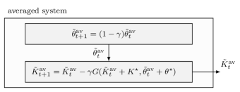
Figure 4: Block diagram of (31) with $\tilde{\mathrm{z}}^{\textsc{av}}_{t}=\operatorname{col}(\tilde{\theta}^{\textsc{av}}_{t},\tilde{K}^{\textsc{av}}_{t})$.

The dynamics of $\tilde{\theta}^{\textsc{av}}_{t}$ is trivially exponentially convergent to zero, while in the following we will formally show that the dynamics of $\tilde{K}^{\textsc{av}}_{t}$ is input-to-state (ISS) exponentially stable (cf. [51]).

For the sake of compactness, let us also introduce the (averaged) estimates $A^{\textsc{av}}_{t}\in\mathbb{R}^{{n}\times{n}}$ and $B^{\textsc{av}}_{t}\in\mathbb{R}^{{n}\times{m}}$ of the matrices $A$ and $B$, defined as

$$\begin{bmatrix}A^{\textsc{av}}_{t}&B^{\textsc{av}}_{t}\end{bmatrix}^{\top}:=\tilde{\theta}^{\textsc{av}}_{t}+\theta^{\star},$$ (32)

where we recall that $\tilde{\theta}^{\textsc{av}}_{t}$ is the first component of $\tilde{\mathrm{z}}^{\textsc{av}}_{t}$. Under the same assumptions of Theorem 3.2, the next result establishes exponential stability of the origin for (31).

Proposition 4.3

Let the assumptions of Theorem 3.2 hold true. Consider the averaged system (31). Then, for all $\tilde{\mathrm{z}}^{\textsc{av}}_{0}\in\mathbb{R}^{(n+2m)\times n}$ such that the corresponding $A^{\textsc{av}}_{0}+B^{\textsc{av}}_{0}(\tilde{K}^{\textsc{av}}_{0}+K^{\star})$ and $A+B(\tilde{K}^{\textsc{av}}_{0}+K^{\star})$ are Schur matrices, there exists $\bar{\gamma}^{\textsc{av}}>0$ such that, for all $\gamma\in(0,\bar{\gamma}^{\textsc{av}})$, the origin of (31) is exponentially stable. $\blacksquare$

The proof of Proposition 4.3 is given in Appendix D.

Once this result has been posed, we can proceed with the proof of Theorem 3.2 in the next subsection.

4.3 Proof of Theorem 3.2

We will use Theorem A.6 given in Appendix A to guarantee the exponential stability of the origin for (25). Specifically, in order to apply Theorem A.6, we need to verify

1. the exponential stability of the origin for the associated averaged system,

2. the Lipschitz continuity of the vector field of (25),

3. that the origin is an equilibrium point of (25), and

4. that

   $$\left\|\dfrac{1}{T}\sum_{\tau=\bar{t}+1}^{\bar{t}+T}\Delta f(\tilde{\mathrm{z}},\tau)\right\|\leq\nu(T)\left\|\tilde{\mathrm{z}}\right\| \left\|\dfrac{1}{T}\sum_{\tau=\bar{t}+1}^{\bar{t}+T}\frac{\partial\tilde{f}(\tilde{\mathrm{z}},\tau)}{\partial\tilde{\mathrm{z}}}\right\|\leq\nu(T),$$ (33)

   where $\Delta f(\tilde{\mathrm{z}},\tau):=f(0,\tilde{\mathrm{z}},\tau)-f^{\textsc{av}}(\tilde{\mathrm{z}})$ and $\nu(t)$ is a nonnegative strictly decreasing function with the property $\nu(t)\to 0$ as $t\to\infty$.

As for condition (i), it follows from Proposition 4.3. Condition (ii) is satisfied by using the quantities defined in (D.3) in Appendix D as the required Lipschitz constants of the vector field of (25). Condition (iii) can be verified by means of (29). Finally, in order to check condition (iv) (cf. (33)), note that

$$\tilde{f}(\tilde{\mathrm{z}},t)=(H^{{\textnormal{ss}}}_{t})^{\dagger}H^{{\textnormal{ss}}}_{t}\tilde{\theta}-\tilde{\theta}\stackrel{{\scriptstyle(a)}}{{=}}0,$$ (34)

where in $(a)$ we use the fact that $H^{{\textnormal{ss}}}_{t}$ is invertible for all $t\in N$ (cf. Lemma C.1 in Appendix D). Therefore, the conditions in (33) are satisfied and, thus, we can apply Theorem A.6. This result guarantees the existence of $\bar{\gamma}>0$ such that, for all $\gamma\in(0,\bar{\gamma})$, the origin is an exponentially stable equilibrium point for system (25). The proof follows backtracking to the original coordinates $(\mathrm{x},\theta,K)$.

5 Numerical Simulations

In this section, we provide some numerical simulations to corroborate our theoretical findings. We consider the linear model of a highly maneuverable aircraft derived from the linearization of its longitudinal dynamics at an altitude of $3000$ $[$ft$]$ and a velocity of $0.6$ $[$Mach$]$, see [52]. The resulting linear time-invariant dynamics in continuous-time reads as

$$\begin{split}\dot{x}=&\left[\begin{smallmatrix}-0.0151&-60.5651&0&-32.174\\ -0.0001&-1.3411&0.9929&0\\ 0.00018&43.2541&-0.86939&0\\ 0&0&1&0\end{smallmatrix}\right]x+\left[\begin{smallmatrix}-2.516&-13.136\\ -0.1689&-0.2514\\ -17.251&-1.5766\\ 0&0\end{smallmatrix}\right]u,\end{split}$$ (35)

where the state $x\in\mathbb{R}^{4}$ represents the forward velocity, the attack angle, the pitch rate and the pitch angle, while the inputs $u\in\mathbb{R}^{2}$ are the elevator and flaperon angles. The discrete-time system matrices ${A}_{\star}$ and ${B}_{\star}$ of (1b) are discretized from the continuous-time system (35) using a Zero Order Hold on the input with sampling time $T_{s}=0.05$ $[$s$]$. Notice that the resulting matrix ${A}_{\star}$ has one eigenvalue outside the unit disk, i.e., it is not Schur. The cost matrices $Q\in\mathbb{R}^{4\times 4}$ and $R\in\mathbb{R}^{2\times 2}$ are randomly generated, while ensuring that $Q=Q^{\top}\geq 0$ and $R=R^{\top}>0$. We set $\gamma=10^{-4}$ and $\left\|\mathrm{w}_{0}\right\|=0.01$.

5.1 Exogenus System Design Procedure

Before providing the results of the numerical simulations, we propose a procedure tailored to design an exogenous system such that Assumption 3.1 is guaranteed. For the sake of completeness, we consider the general case with the state dimension being ${n}$ and the input dimension being ${m}$. First, we set $q:=n+1$, $n_{\mathrm{w}}=qm$, and $F:=\operatorname{blkdiag}(F_{1},\dots,F_{q}),$ where, for all $i\in\{1,\ldots,q\}$,

$$F_{i}:=\begin{bmatrix}\cos(\omega_{i})&\sin(\omega_{i})\\ -\sin(\omega_{i})&\cos(\omega_{i})\end{bmatrix},$$

for some given $\omega_{i}>0$ such that $\omega_{i}$ and $\omega_{j}$ are uncorrelated for each pair $i,j\in\{1,\ldots,q\}$ with $i\neq j$. By choosing an initial condition $\mathrm{w}_{0}$ that satisfies

$$([\mathrm{w}_{0}]_{2i+1})^{2}+([\mathrm{w}_{0}]_{2i+2})^{2}\neq 0,\quad 0\leq i\leq q-1,$$ (36)

the chosen structure of $F$ guarantees (14a) according to [53, Th.2]. As for (14b), we achieve it by selecting $E$ such that $\begin{bmatrix}E^{\top}&(EF)^{\top}&\ldots&(EF^{n})^{\top}\end{bmatrix}$ is nonsingular.

5.2 Aircraft Control

We start by considering the LTI system (35). We run Relearn LQR with the exogenus signal generated via the procedure detailed above. In Figure 6 (left) it is possible to observe the evolution of the normalized cost error $|J(K_{t},\theta^{\star}_{t})-J^{\star}|/J^{\star}$, with $J^{\star}:=J(K^{\star},\theta^{\star})$ and $\theta^{\star}:=[{A}_{\star}\;{B}_{\star}]^{\top}$, in logarithmic scale. On the right of Figure 6 it is depicted the evolution of the normalized estimation error $\left\|\theta_{t}-\theta^{\star}\right\|/\left\|\theta^{\star}\right\|$ in logarithmic scale. Notice that, in both cases, convergence to the optimal cost $J^{\star}$ and true parameters $\theta^{\star}$ is achieved. Finally, in Figure 5 the state trajectory of the closed-loop system is depicted. The initial condition $\mathrm{x}_{0}$ is sampled from a normal distribution with mean value $10$ for each state. Notice that, after a transient, the states oscillate about the origin due to the exogenous system.

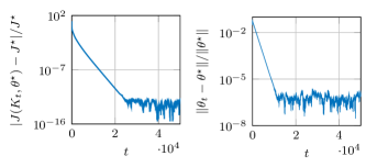
Figure 5: (left) Evolution of the normalized cost error $|J(K_{t},\theta^{\star}_{t})-J^{\star}|/J^{\star}$. (right) Evolution of the normalized estimation error about $\left\|\theta_{t}-\theta^{\star}\right\|/\left\|\theta^{\star}\right\|$ (left).

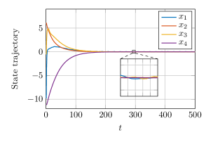
Figure 6: State trajectory of the closed-loop system. The states $x_{1}$, $x_{2}$, $x_{3}$, $x_{4}$ correspond, respectively, the forward velocity, the attack angle, the pitch rate and the pitch angle.

5.3 Aircraft Control with Drifting Parameters

To better highlight the capabilities of our algorithm, we also consider the case where the system matrices ${A}_{\star}$, ${B}_{\star}$, slowly change over time. The new time-varying state and input matrices are denoted as $A^{t}_{\star}$ and $B^{t}_{\star}$, respectively. More in detail, the time-varying system matrices $A^{t}_{\star}$ and $B^{t}_{\star}$ smoothly evolve from ${A}_{\star}$ and ${B}_{\star}$ toward a new pair of matrices $A_{+}$ and $B_{+}$, according to the update law

$$A^{t}_{\star} =(1-\sigma(t)){A}_{\star}+\sigma(t)A_{+}$$

$$B^{t}_{\star} =(1-\sigma(t)){B}_{\star}+\sigma(t)B_{+},$$

for all $t\geq 0$, with $\sigma(t)$ being a sigmoid function defined as $\sigma(t)=1/(1+\exp(\tfrac{t-t^{\text{mid}}}{\alpha}\big{)})$, where $\alpha\in\mathbb{R}$ determines the transition width and $t^{\text{mid}}\in\mathbb{N}$ defining the center of the transition. We select $t^{\text{mid}}=1.5\cdot 10^{5}$ and $\alpha=5\cdot 10^{3}$, while the entries $a_{ij}^{+}$ and $b_{i\ell}^{+}$ of $A_{+}$ and $B_{+}$ are randomly generated according to

$$a_{ij}^{+} =\begin{cases}a_{ij}\quad\quad\quad\quad\text{if }a_{ij}=0\\ a_{ij}+\sigma v_{ij}^{A}\quad\text{otherwise}\end{cases}$$

$$b_{i\ell}^{+} =\begin{cases}b_{i\ell}\quad\quad\quad\quad\text{if }b_{ij}=0\\ b_{i\ell}+\sigma v_{i\ell}^{B}\quad\text{otherwise}\end{cases},$$

for all $i,j\in\{1,\ldots,n\}$ and $\ell\in\{1,\ldots,m\}$, where $v_{ij}^{A}$ and $v_{i\ell}^{B}$ are random variables normally distributed and $\sigma=0.1$ is the chosen variance. In Figure 7, we compare $J(K_{t},\theta^{\star}_{t})$ and $J^{\star}_{t}$. In Figure 8 (right), it is possible to observe the evolution of the normalized cost error $|J(K_{t},\theta^{\star}_{t})-J^{\star}_{t}|/J^{\star}_{t}$, with $J^{\star}_{t}:=J(K^{\star},\theta^{\star}_{t})$ and $\theta^{\star}_{t}:=\begin{bmatrix}A^{t}_{\star}&B^{t}_{\star}\end{bmatrix}^{\top}$, in logarithmic scale. Finally, in Figure 8 (left) it is depicted the evolution of the normalized estimation error $\left\|\theta_{t}-\theta^{\star}_{t}\right\|/\left\|\theta^{\star}_{t}\right\|$ in logarithmic scale. Notice that, in both cases, convergence to the optimal cost $J^{\star}_{t}$ and true parameters $\theta^{\star}_{t}$ is achieved. As one may expect, in the neighborhood of the inflection point $t\approx t^{\text{mid}}$, both error quantities increase. However, we note that our policy shows its adaptability by quickly recovering convergence toward the optimal gain and exact estimation.

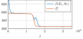
Figure 7: Comparison between $J(K_{t},\theta^{\star}_{t})$ and $J^{\star}_{t}$.

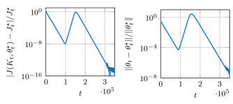
Figure 8: (Left) Evolution of the normalized cost error $|J(K_{t},\theta^{\star}_{t})-J^{\star}_{t}|/J^{\star}_{t}$. (right) Evolution of the normalized estimation error $\left\|\theta_{t}-\theta^{\star}_{t}\right\|/\left\|\theta^{\star}_{t}\right\|$ (left).

6 Conclusions

In this paper, we addressed infinite-horizon LQR problems with unknown state-input matrices. Specifically, we propose a procedure mixing the identification phase of the unknown matrices with the optimization of the feedback policy. We design an iterative algorithm combining a Recursive Least Squares (RLS) scheme (elaborating samples from the closed-loop system persistently excited by a dithering signal) with the gradient method. We proved exponential convergence of the overall procedure to the optimal steady-state associated to the optimal gain and the exact matrices by using tools from Lyapunov-based analysis tools in combination with averaging theory for nonlinear systems.

Appendix A Preliminaries on averaging theory for two-time-scale systems

We report [54, Theorem 2.2.4], which is a useful result in the context of averaging theory for two-time-scale systems. Consider the time-varying system

$$\chi_{t+1} =\mathcal{A}(\mathrm{z}_{t})\chi_{t}+h(\mathrm{z}_{t},t)+\epsilon g(\chi_{t},\mathrm{z}_{t},t)$$ (A.1a)

$$\mathrm{z}_{{t+1}} =\mathrm{z}_{t}+\epsilon f(\chi_{t},\mathrm{z}_{t},t),$$ (A.1b)

with $\chi_{t}\in\mathbb{R}^{n_{\chi}}$, $\mathrm{z}_{t}\in\mathbb{R}^{n_{\mathrm{z}}}$, $g:\mathbb{R}^{n_{\chi}}\times\mathbb{R}^{n_{\mathrm{z}}}\times\mathbb{N}\to\mathbb{R}^{n_{\chi}}$, $f:\mathbb{R}^{n_{\chi}}\times\mathbb{R}^{n_{\mathrm{z}}}\times\mathbb{N}\to\mathbb{R}^{n_{\chi}}$, and $A:\mathbb{R}^{n_{\mathrm{z}}}\to\mathbb{R}^{n_{\chi}\times n}$. We enforce the following assumptions.

Assumption A.1

There exists $r$ such that $f$, $g$, and $h$ are Lipschitz continuous into $\mathcal{B}_{r}(0_{n_{\chi}+n_{\mathrm{z}}})$. $\blacksquare$

Assumption A.2

It holds $h(0,t)=0$, $g(0,0,t)=0$, and $f(0,0,t)=0$ for all $t\in\mathbb{N}$. $\blacksquare$

Assumption A.3

There exist $r,m_{1},m_{2}>0$ and $a_{1},a_{2}\in(0,1)$ such that, for all $\mathrm{z}\in\mathcal{B}_{r}(0_{n_{\mathrm{z}}})$ and $t\in\mathbb{N}$, it holds

$$m_{1}a_{1}^{t}\leq\left\|\mathcal{A}(\mathrm{z})^{t}\right\|\leq m_{2}a_{2}^{t},$$

Moreover, there exists $k_{a}>0$ such that

$$\left\|\dfrac{\partial\mathcal{A}(\mathrm{z})}{\partial\mathrm{z}_{i}}\right\|\leq k_{a},$$

for all $i\in\{1,\ldots,m\}$ and $\mathrm{z}\in\mathcal{B}_{r}(0_{n_{\mathrm{z}}})$. $\blacksquare$

Assumption A.4

The function $f$ is piecewise continuous in $t$ with the limit

$$f^{\textsc{av}}(\mathrm{z}):=\lim_{T\to\infty}\frac{1}{T}\sum_{\tau=\bar{t}+1}^{\bar{t}+T}f(0,\mathrm{z},\tau)$$ (A.2)

existing uniformly in $\bar{t}\in\mathbb{N}$ and for all $\mathrm{z}\in\mathcal{B}_{r}(0_{n_{\mathrm{z}}})$. $\blacksquare$

We associate a so-called averaged system to (A.1) given by

$$\mathrm{z}^{\textsc{av}}_{t+1}=\mathrm{z}^{\textsc{av}}_{t}+\epsilon f^{\textsc{av}}(\mathrm{z}^{\textsc{av}}_{t}).$$ (A.3)

Assumption A.5

Consider $f^{\textsc{av}}$ as defined in (A.2) and let $\Delta f:\mathbb{R}^{n_{\mathrm{z}}}\times\mathbb{N}\to\mathbb{R}^{n_{\mathrm{z}}}$ be defined as

$$\Delta f(\mathrm{z},t):=f(0,\mathrm{z},t)-f^{\textsc{av}}(\mathrm{z}).$$

Then, there exists a nonnegative strictly decreasing function $\nu(t)$ such that $\lim_{t\to\infty}\nu(t)=0$ and

$$\left\|\dfrac{1}{T}\sum_{\tau=\bar{t}+1}^{\bar{t}+T}\tilde{f}(\mathrm{z},\tau)\right\| \leq\nu(T)\left\|\mathrm{z}\right\|$$

$$\left\|\dfrac{1}{T}\sum_{\tau=\bar{t}+1}^{\bar{t}+T}\frac{\partial\tilde{f}(\mathrm{z},\tau)}{\partial\mathrm{z}}\right\| \leq\nu(T),$$

uniformly in $\bar{t}\in\mathbb{N}$ and for all $\mathrm{z}\in\mathcal{B}_{r}(0_{n_{\mathrm{z}}})$. $\blacksquare$

Theorem A.6

[54, Theorem 2.2.4] Consider system (A.1) and let Assumptions A.1, A.2, A.3, A.4 and A.5 hold. If there exists $\epsilon_{0}>0$ such that, for all $\epsilon\in(0,\epsilon_{0})$, the origin is exponentially stable for system (A.3), then there exists $\epsilon_{1}>0$ such that, for all $\epsilon\in(0,\epsilon_{1})$, the origin is an exponentially stable equilibrium of system (A.1). $\blacksquare$

Appendix B Proof of Lemma 4.1

We note that (22) is obtained by setting $K_{t}=K^{\star}$ in (19) (which compactly collects the updates (15a), (15b), and (18)). Hence, we start by inspecting (15a) and (15b) restricted to the manifold in which $K_{t}=K^{\star}$, namely

$$\mathrm{w}_{{t+1}} =F\mathrm{w}_{t}$$ (B.1a)

$$\mathrm{\mathrm{x}}_{{t+1}} =({A}_{\star}+{B}_{\star}K^{\star})\mathrm{\mathrm{x}}_{t}+{B}_{\star}E\mathrm{w}_{t}.$$ (B.1b)

System (B.1) is a cascade, therefore its steady-state solution is $\operatorname{col}(\mathrm{w}_{t},\mathrm{\mathrm{x}}_{t})=\operatorname{col}(I_{n_{\mathrm{w}}},\Pi_{\mathrm{x}})\mathrm{w}_{t}$, with $\Pi_{\mathrm{x}}\in\mathbb{R}^{n\times m}$ solution to the following Sylvester equation

$$\Pi_{\mathrm{x}}F=({A}_{\star}+{B}_{\star}K^{\star})\Pi_{\mathrm{x}}+{B}_{\star}E.$$ (B.2)

Being $F$ marginally stable (cf. Assumption 3.1) and ${A}_{\star}+{B}_{\star}K^{\star}$ Schur (so that $\sigma(F)\cap\sigma({A}_{\star}+{B}_{\star}K^{\star})=\emptyset$) the solution $\Pi_{\mathrm{x}}$ exists and is unique. Then, we inspect the dynamics (18) restricted to the manifold in which $\mathrm{\mathrm{x}}_{t}=\Pi_{\mathrm{x}}\mathrm{w}_{t}$ and $K_{t}=K^{\star}$. Let $M\in\mathbb{R}^{(n+m)\times(n+m)}$ be

$$M:=\begin{bmatrix}\Pi_{\mathrm{x}}^{\top}&(K^{\star}\Pi_{\mathrm{x}}+E)^{\top}\end{bmatrix}^{\top},$$ (B.3)

then it holds

$$\mathtt{vec}\left(\mathrm{w}_{{t+1}}\mathrm{w}_{{t+1}}^{\top}\right)=\mathtt{vec}\left(F\mathrm{w}_{t}\mathrm{w}_{t}^{\top}F^{\top}\right)$$ (B.4a)

$$H^{\text{vc}}_{t+1}=\lambda H^{\text{vc}}_{t}+\mathtt{vec}\left(M\mathrm{w}_{t}\mathrm{w}_{t}^{\top}M^{\top}\right)$$ (B.4b)

$$S^{\text{vc}}_{t+1}=\lambda S^{\text{vc}}_{t}+\mathtt{vec}\left(M\mathrm{w}_{t}\mathrm{w}_{t}^{\top}M^{\top}\theta^{\star}\right),$$ (B.4c)

where the first equation comes from the vectorization of (15a). By exploiting the vectorization properties, we can manipulate (B.4) to obtain the system

$$\mathtt{vec}\!\left(\mathrm{w}_{{t+1}}\mathrm{w}_{{t+1}}^{\top}\right)\!=\!(F\otimes F)\mathtt{vec}\left(\mathrm{w}_{t}\mathrm{w}_{t}^{\top}\right)$$ (B.5a)

$$H^{\text{vc}}_{t+1}\!=\!\lambda H^{\text{vc}}_{t}\!+\!(M\otimes M)\mathtt{vec}\left(\mathrm{w}_{t}\mathrm{w}_{t}^{\top}\right)$$ (B.5b)

$$S^{\text{vc}}_{t+1}\!=\!\lambda S^{\text{vc}}_{t}\!+\!({\theta^{\star}}^{\top}\!M\!\otimes\!M)\mathtt{vec}\left(\mathrm{w}_{t}\mathrm{w}_{t}^{\top}\right)\!,$$ (B.5c)

which enjoys again a cascade structure. Thus, let $\Pi_{H}\in\mathbb{R}^{(n+m)^{2}\times n_{\mathrm{w}}^{2}}$ and $\Pi_{S}\in\mathbb{R}^{(n+m)n\times n_{\mathrm{w}}^{2}}$ be the solution to the Sylvester equations associated to the cascade in (B.5) given by

$$\Pi_{H}(F\otimes F) =\lambda\Pi_{H}+M\otimes M$$ (B.6a)

$$\Pi_{S}(F\otimes F) =\lambda\Pi_{S}+({\theta^{\star}}^{\top}M)\otimes M.$$ (B.6b)

Being $F$ marginally stable (cf. Assumption 3.1) and $\lambda\in(0,1)$, then $\sigma(F\otimes F)\cap\sigma(\lambda I)=\emptyset$ and, thus, the solutions $\Pi_{S}$ and $\Pi_{H}$ to (B.6) exist and are unique. The proof of (22) follows by (i) noticing that $(\Pi_{\mathrm{x}},\Pi_{H},\Pi_{S})$ are used to define $\chi^{{\textnormal{ss}}}$ (cf. (21)), and (ii) plugging (B.2) and (B.6) into system (19).

As for (23), it can be shown using an algebraic manipulation of (B.6). Indeed, by pre-multiplying (B.6a) by ${\theta^{\star}}^{\top}\otimes I_{n+m}$ we can write

$$({\theta^{\star}}^{\top}\!\otimes\!I_{n+m})\Pi_{H}(F\otimes F-\lambda I) \!=\!({\theta^{\star}}^{\top}\otimes I_{n+m})(M\otimes M)$$

$$\!\stackrel{{\scriptstyle(a)}}{{=}}\!({\theta^{\star}}^{\top}M)\otimes M$$

$$\!\stackrel{{\scriptstyle(b)}}{{=}}\!\!\Pi_{S}(\!F\!\otimes\!F\!-\!\lambda I),$$ (B.7)

where in $(a)$ we used the mixed-product property of the Kronecker operator, while $(b)$ follows from (B.6b). So that the proof is complete.

Appendix C Proof of Lemma 4.2

Before proving Lemma 4.2, we need the following result that shows that $H^{{\textnormal{ss}}}_{t}$ is invertible for all $t\in\mathbb{N}$. We recall that $H^{{\textnormal{ss}}}_{t}$ is the unvectorized version of the second block-component of $\chi^{{\textnormal{ss}}}(\mathrm{w}_{t})$ (see (21) and (27)).

Lemma C.1

Let the assumptions of Theorem 3.2 hold true. Then, the matrix $H^{{\textnormal{ss}}}_{t}$, defined in (27), is invertible for all $t\in\mathbb{N}$. $\blacksquare$

Proof C.2

We will prove the invertibility property of the matrix $H^{{\textnormal{ss}}}_{t}$ by investigating the evolution of $H_{t}$. The dynamics of $H_{t}$ in (15c) restricted to the manifold in which $\mathrm{\mathrm{x}}_{t}=\Pi_{\mathrm{x}}\mathrm{w}_{t}$ and $K_{t}=K^{\star}$ reads as

$$H_{{t+1}}=\lambda H_{t}+M\mathrm{w}_{t}\mathrm{w}_{t}^{\top}M^{\top},$$ (C.1)

with $M$ as in (B.3). The explicit solution of (C.1) is

$$H_{t}=\lambda^{t}H_{0}+M\underbrace{\left(\sum_{\tau=0}^{t-1}\lambda^{t-1-\tau}\mathrm{w}_{\tau}\mathrm{w}_{\tau}^{\top}\right)}_{\mathcal{W}_{t}}M^{\top}.$$ (C.2)

Being $\lambda\in(0,1)$, the free evolution $\lambda^{t}H_{0}$ in (C.2) vanishes as $t\to\infty$. Hence, it does not impact on the invertibility of the steady-state solution.

Therefore, let us focus on the forced response $M\mathcal{W}_{t}M^{\top}$ only. We first notice that $\alpha_{1}I_{n_{\mathrm{w}}}\leq\sum_{\tau=\bar{t}+1}^{\bar{t}+t_{\mathrm{w}}}\mathrm{w}_{\tau}\mathrm{w}_{\tau}^{\top}\leq\alpha_{2}I_{n_{\mathrm{w}}}$ for all $\bar{t}\in\mathbb{N}$ (cf. Assumption 3.1). Hence we can invoke [55, Lemma 1] to assert the positive definiteness of $\mathcal{W}_{t}$ for all $t\geq t_{\mathrm{w}}$. Let us consider the Cholesky decomposition of $\mathcal{W}_{t}$ given by $\mathcal{W}_{t}=\mathcal{C}_{t}\mathcal{C}_{t}^{\top}$, with $\mathcal{C}_{t}\in\mathbb{R}^{n_{\mathrm{w}}\times n_{\mathrm{w}}}$ invertible. Then, for all $t\geq t_{\mathrm{w}}$, we can write

$$\operatorname{rank}\left(M\mathcal{W}_{t}M^{\top}\right) =\operatorname{rank}(M\mathcal{C}_{t})\stackrel{{\scriptstyle(a)}}{{=}}\operatorname{rank}(M),$$ (C.3)

where in $(a)$ we used the full-rankness of $\mathcal{C}_{t}$ and a property of the rank operator. To compute $\operatorname{rank}(M)$, we consider again the dynamics in (15a) and (15b) restricted to the manifold in which $K_{t}=K^{\star}$, namely

$$\mathrm{w}_{{t+1}} =F\mathrm{w}_{t}$$ (C.4a)

$$\mathrm{\mathrm{x}}_{{t+1}} =({A}_{\star}+{B}_{\star}K^{\star})\mathrm{\mathrm{x}}_{t}+{B}_{\star}E\mathrm{w}_{t}.$$ (C.4b)

Recalling that $\mathrm{d}_{t}=E\mathrm{w}_{t}$ satisfies condition (14b) (cf. Assumption 3.1) and that $({A}_{\star},{B}_{\star})$ is controllable (cf. Assumption 2.1), we can invoke [48, Cor. 2] to claim that

$$\operatorname{rank}\left(\begin{bmatrix}\mathrm{x}_{0}&\dots&\mathrm{x}_{\mathbf{t}_{\mathrm{d}}-1}\\ \mathrm{d}_{0}&\dots&\mathrm{d}_{\mathbf{t}_{\mathrm{d}}-1}\end{bmatrix}\right)=n+m,$$ (C.5)

for all $(\mathrm{x}_{0},\mathrm{d}_{0})\in\mathbb{R}^{n}\times\mathbb{R}^{m}$. When the initial condition of (C.4b) lies in the invariant steady-state locus (cf. (B.2)), i.e., when $\mathrm{x}_{0}=\Pi_{\mathrm{x}}\mathrm{w}_{0}$, the condition in (C.5) simplifies to

$$\operatorname{rank}\left(M\begin{bmatrix}\mathrm{w}_{0}&\dots&\mathrm{w}_{\mathbf{t}_{\mathrm{d}}-1}\end{bmatrix}\right)=n+m,$$ (C.6)

with $M$ as in (B.3), which allows us to conclude that

$$\operatorname{rank}(M)\geq n+m.$$

Moreover, being $\operatorname{rank}(M)\leq n+m$ by construction, the above inequality yields to $\operatorname{rank}(M)=n+m$, which, in turn, combined with (C.3), allows us to write

$$\operatorname{rank}\left(M\mathcal{W}_{t}M^{\top}\right)=n+m,$$ (C.7)

for all $t\geq t_{\mathrm{w}}$. Next, we characterize the $\operatorname{rank}(M\mathcal{W}_{t}M^{\top})$ after the transient phase. Being $\lambda\in(0,1)$, it holds that $M\mathcal{W}_{t}M^{\top}$ exponentially converges to $H^{{\textnormal{ss}}}_{t}$. Hence, by continuity, there must exist $t_{\infty}\geq t_{\mathrm{w}}$ such that

$$\operatorname{rank}(H^{{\textnormal{ss}}}_{t})=n+m,$$

for all $t\geq t_{\infty}$. Finally, being $H^{{\textnormal{ss}}}_{t}$ a static function of the periodic signal $\mathrm{w}_{t}$, then $H^{{\textnormal{ss}}}_{t}$ is periodic as well so that its full-rankness is independent of $t$. Thus, it must be that $\operatorname{rank}(H^{{\textnormal{ss}}}_{t})=n+m$ for all $t\in\mathbb{N}$, and the proof follows. $\blacksquare$

Once the invertibility of $H^{{\textnormal{ss}}}_{t}$ has been established by Lemma C.1, we are ready to prove Lemma 4.2. Let us label the two components of $f^{\textsc{av}}$ as

$$\begin{bmatrix}f^{\textsc{av}}_{1}(\tilde{\mathrm{z}})\\ f^{\textsc{av}}_{2}(\tilde{\mathrm{z}})\end{bmatrix}:=\lim_{T\to\infty}\frac{1}{T}\sum_{\tau=\bar{t}+1}^{\bar{t}+T}f(0,\tilde{\mathrm{z}},\tau).$$

As for $f^{\textsc{av}}_{1}(\mathrm{z})$, we can write

$$f^{\textsc{av}}_{1}(\tilde{\mathrm{z}}) =-\lim_{T\to\infty}\frac{1}{T}\sum_{\tau=\bar{t}+1}^{\bar{t}+T}(H^{{\textnormal{ss}}}_{\tau})^{\dagger}H^{{\textnormal{ss}}}_{\tau}\tilde{\theta}\stackrel{{\scriptstyle(a)}}{{=}}-\tilde{\theta},$$

where in $(a)$ we used Lemma C.1 to guarantee the invertibility of $H^{{\textnormal{ss}}}_{t}$ for all $t\in\mathbb{N}$ . As for $f^{\textsc{av}}_{2}(\mathrm{z})$, its existence is trivially shown by observing that it does not depend on $t$. Hence, given $\tilde{\mathrm{z}}=\operatorname{col}(\tilde{K},\tilde{\theta})$, it holds

$$f^{\textsc{av}}_{2}(\tilde{\mathrm{z}}):=-G(\tilde{K}+K^{\star},\tilde{\theta}+\theta^{\star}).$$

Appendix D Proof of Proposition 4.3

The proof resorts to a suitable Lyapunov candidate function whose increment along trajectories of system (31) will allow us to claim exponential stability of the origin.

To ease the notation, we start by decomposing the state of (31) as $\tilde{\mathrm{z}}^{\textsc{av}}_{t}:=\operatorname{col}(\tilde{\theta}^{\textsc{av}}_{t},\tilde{K}^{\textsc{av}}_{t})$. Then, we recall [30, Lemma 3.12] to guarantee that the cost $J$, defined in (5), is gradient dominated, that is for all $K\in\mathcal{D}$ it holds

$$J(K,\theta^{\star})-J(K^{\star},\theta^{\star})\leq\mu\left\|G(K,\theta^{\star})\right\|^{2},$$ (D.1)

for some $\mu>0$, where $G$ denotes the gradient of $J$. Now, let us consider the Lyapunov candidate function $V:\mathbb{R}^{m\times n}\times\mathbb{R}^{(n+m)\times n}\to\mathbb{R}$ defined as

$$V(\tilde{K}^{\textsc{av}},\tilde{\theta}^{\textsc{av}}):=$$ (D.2)

$$\hskip 22.76228pt\kappa\left(J(\tilde{K}^{\textsc{av}}+K^{\star},\theta^{\star})-J(K^{\star},\theta^{\star})\right)+\tfrac{1}{2}\left\|\tilde{\theta}^{\textsc{av}}\right\|^{2},$$

with $\kappa>0$, whose specific value will be set later. Being $K^{\star}$ the unique minimizer of $J(\cdot,\theta^{\star})$ [30], we note that $V$ is positive definite. Now, given any $c>0$, let us introduce the level set $\Omega_{c}\subset\mathbb{R}^{{m}\times{m}}\times\mathbb{R}^{(n+m)\times n}$ of $V$, defined as

$$\Omega_{c}:=\Big{\{}(\tilde{K}^{\textsc{av}},\tilde{\theta}^{\textsc{av}})\in\mathbb{R}^{m\times n}\times\mathbb{R}^{(n+m)\times n}\mid$$

$$\hskip 45.52458ptJ(\tilde{K}^{\textsc{av}}+K^{\star},\theta^{\star})-J(K^{\star},\theta^{\star})+\tfrac{1}{2}\left\|\tilde{\theta}^{\textsc{av}}\right\|^{2}\leq c\Big{\}}.$$

Let $c_{0}>0$ be the smallest number such that $(\tilde{K}^{\textsc{av}}_{0},\tilde{\theta}^{\textsc{av}}_{0})\in\Omega_{c_{0}}$ and define

$$\beta_{1}\! :=\!\!\max_{(\tilde{K}^{\textsc{av}},\tilde{\theta}^{\textsc{av}})\in\Omega_{c_{0}}}\!\!\left\{\left\|\dfrac{\partial G(\tilde{K}^{\textsc{av}}\!+\!K^{\star},\tilde{\theta}^{\textsc{av}}\!+\!\theta^{\star})}{\partial\tilde{K}^{\textsc{av}}}\right\|\right\}$$ (D.3a)

$$\beta_{2}\! :=\!\!\max_{(\tilde{K}^{\textsc{av}},\tilde{\theta}^{\textsc{av}})\in\Omega_{c_{0}}}\!\!\left\{\left\|\dfrac{\partial G(\tilde{K}^{\textsc{av}}\!+\!K^{\star},\tilde{\theta}^{\textsc{av}}\!+\!\theta^{\star})}{\partial\tilde{\theta}^{\textsc{av}}}\right\|\right\}\!\!.$$ (D.3b)

Indeed, we recall that (i) $\theta_{0}^{\textsc{av}}=\theta_{0}\in\Theta_{b}$ and (ii) the corresponding closed-loop matrix $(A_{0}^{\textsc{av}}+B_{0}^{\textsc{av}}K_{0}^{\textsc{av}})=(A_{0}+B_{0}K_{0})$ is Schur. Thus, in light of [30, Proposition 3.10], it holds that $\frac{\partial G(\tilde{K}^{\textsc{av}}+K^{\star},\tilde{\theta}^{\textsc{av}}+\theta^{\star})}{\partial\tilde{K}^{\textsc{av}}}$ is a continuous function of the gains $(\tilde{K}^{\textsc{av}}+K^{\star})$ stabilizing for $({A}_{t}^{\textsc{av}},{B}_{t}^{\textsc{av}})$. Similarly, also continuity of $\frac{\partial G(\tilde{K}^{\textsc{av}}\!+\!K^{\star},\tilde{\theta}^{\textsc{av}}\!+\!\theta^{\star})}{\partial\tilde{\theta}^{\textsc{av}}}$ with respect to $(\tilde{\theta}^{\textsc{av}}+\theta^{\star})\in\Theta_{b}$ can be shown. Hence, $(\beta_{1},\beta_{2})$ are well posed, i.e., finite. We remark that [30, Corolllary 3.7.1] guarantees that, given any $c>0$, the level set of the cost function $J$, namely $\{\tilde{K}\in\mathbb{R}^{m\times n}\mid J(\tilde{K}^{\textsc{av}}+K^{\star},\theta^{\star})-J(K^{\star},\theta^{\star})\leq c\}\subset\mathbb{R}^{m\times n}$, is compact and, thus, so is $\Omega_{c}$.

Next, we show that $\Omega_{c_{0}}$ is (forward) invariant for (31). To this end, assume that $(\tilde{K}^{\textsc{av}}_{t},\tilde{\theta}^{\textsc{av}}_{t})\in\Omega_{c_{0}}$ and let us prove the invariance of $\Omega_{c_{0}}$ using an induction argument.

Recall that, the cost $J(\tilde{K}^{\textsc{av}}_{t}+K^{\star},\tilde{\theta}^{\textsc{av}}_{t}+\theta^{\star})$ is finite for all $\tilde{\mathrm{z}}^{\textsc{av}}_{t}\in\Omega_{c_{0}}$, and, hence, iteration (31) is well-posed. The increment $\Delta V$ of $V$ along trajectories of (31) is given by

$$\Delta V(\tilde{K}^{\textsc{av}}_{t},\tilde{\theta}^{\textsc{av}}_{t}):=V(\tilde{K}^{\textsc{av}}_{{t+1}},\tilde{\theta}^{\textsc{av}}_{{t+1}})-V(\tilde{K}^{\textsc{av}}_{t},\tilde{\theta}^{\textsc{av}}_{t})$$

$$=\kappa\Big{(}J(\tilde{K}^{\textsc{av}}_{{t+1}}+K^{\star},\theta^{\star})-J(\tilde{K}^{\textsc{av}}_{t}+K^{\star},\theta^{\star})\Big{)}$$

$$\hskip 11.38092pt-\gamma\left(1-\gamma/2\right)\left\|\tilde{\theta}^{\textsc{av}}_{t}\right\|^{2}$$

$$\stackrel{{\scriptstyle(a)}}{{\leq}}\kappa J(\tilde{K}^{\textsc{av}}_{t}+K^{\star}-\gamma G(\tilde{K}^{\textsc{av}}_{t}+K^{\star},\tilde{\theta}^{\textsc{av}}_{t}+\theta^{\star}),\theta^{\star})$$

$$\hskip 11.38092pt-\kappa J(\tilde{K}^{\textsc{av}}_{t}+K^{\star}-\gamma G(\tilde{K}^{\textsc{av}}_{t}+K^{\star},\theta^{\star}),\theta^{\star})$$

$$\hskip 11.38092pt+\kappa J(\tilde{K}^{\textsc{av}}_{t}+K^{\star}-\gamma G(\tilde{K}^{\textsc{av}}_{t}+K^{\star},\theta^{\star}),\theta^{\star})$$

$$\hskip 11.38092pt-\kappa J(\tilde{K}^{\textsc{av}}_{t}+K^{\star},\theta^{\star})-\gamma\left(1-\gamma/2\right)\left\|\tilde{\theta}^{\textsc{av}}_{t}\right\|^{2}$$

$$\stackrel{{\scriptstyle(b)}}{{\leq}}\kappa J(\tilde{K}^{\textsc{av}}_{t}+K^{\star}-\gamma G(\tilde{K}^{\textsc{av}}_{t}+K^{\star},\tilde{\theta}^{\textsc{av}}_{t}+\theta^{\star}),\theta^{\star})$$

$$\hskip 11.38092pt-\kappa J(\tilde{K}^{\textsc{av}}_{t}+K^{\star}-\gamma G(\tilde{K}^{\textsc{av}}_{t}+K^{\star},\theta^{\star}),\theta^{\star})$$

$$\hskip 11.38092pt-\gamma\kappa\left(1-\gamma\tfrac{\beta_{1}}{2}\right)\left\|G(\tilde{K}^{\textsc{av}}_{t}+K^{\star},\theta^{\star})\right\|^{2}$$

$$\hskip 11.38092pt-\gamma\left(1-\gamma/2\right)\left\|\tilde{\theta}^{\textsc{av}}_{t}\right\|^{2}\!,$$ (D.4)

where $(a)$ uses the update of $\tilde{K}^{\textsc{av}}_{{t+1}}$ and adds $\pm\kappa J(\tilde{K}^{\textsc{av}}_{t}+K^{\star}-\gamma G(\tilde{K}^{\textsc{av}}_{t}+K^{\star},\theta^{\star}),\theta^{\star})$, $(b)$ uses the Taylor expansion of $J(\cdot,\cdot)$ about $(\tilde{K}^{\textsc{av}}_{t}+K^{\star},\theta^{\star})$ evaluated at $(\tilde{K}^{\textsc{av}}_{t}+K^{\star}-\gamma G(\tilde{K}^{\textsc{av}}_{t}+K^{\star},\theta^{\star}),\theta^{\star})$ and uses (D.3a).

Next, we manipulate the difference between the first two terms in (D.4). By expanding $J(\cdot,\cdot)$ about $(\tilde{K}^{\textsc{av}}_{t}+K^{\star},\theta^{\star})$ evaluated at $(\tilde{K}^{\textsc{av}}_{t}+K^{\star}-\gamma G(\tilde{K}^{\textsc{av}}_{t}+K^{\star},\tilde{\theta}^{\textsc{av}}_{t}+\theta^{\star}),\theta^{\star})$ and $(\tilde{K}^{\textsc{av}}_{t}+K^{\star}-\gamma G(\tilde{K}^{\textsc{av}}_{t}+K^{\star},\theta^{\star}),\theta^{\star})$ and using (D.3a) and the Cauchy-Schwarz inequality, we can write

$$J(\tilde{K}^{\textsc{av}}_{t}+K^{\star}-\gamma G(\tilde{K}^{\textsc{av}}_{t}+K^{\star},\tilde{\theta}^{\textsc{av}}_{t}+\theta^{\star}),\theta^{\star})$$

$$\hskip 11.38092pt-J(\tilde{K}^{\textsc{av}}_{t}+K^{\star}-\gamma G(\tilde{K}^{\textsc{av}}_{t}+K^{\star},\theta^{\star}),\theta^{\star})$$

$$\leq\gamma\left\|G(\tilde{K}^{\textsc{av}}_{t}+K^{\star},\theta^{\star})\right\|\!$$

$$\hskip 28.45274pt\cdot\left\|G(\tilde{K}^{\textsc{av}}_{t}\!+\!K^{\star},\tilde{\theta}^{\textsc{av}}_{t}\!+\!\theta^{\star})\!-\!G(\tilde{K}^{\textsc{av}}_{t}\!+\!K^{\star},\theta^{\star})\right\|$$

$$\hskip 11.38092pt+\tfrac{\gamma^{2}\beta_{1}}{2}\left\|G(\tilde{K}^{\textsc{av}}_{t}\!+\!K^{\star},\tilde{\theta}^{\textsc{av}}_{t}\!+\!\theta^{\star})\right\|^{2}$$

$$\hskip 11.38092pt+\tfrac{\gamma^{2}\beta_{1}}{2}\left\|G(\tilde{K}^{\textsc{av}}_{t}\!+\!K^{\star},\theta^{\star})\right\|^{2}$$

$$\stackrel{{\scriptstyle(a)}}{{\leq}}\gamma\beta_{2}\left\|G(\tilde{K}^{\textsc{av}}_{t}+K^{\star},\theta^{\star})\right\|\left\|\tilde{\theta}^{\textsc{av}}_{t}\right\|$$

$$\hskip 11.38092pt+\tfrac{\gamma^{2}\beta_{1}}{2}\left\|G(\tilde{K}^{\textsc{av}}_{t}+K^{\star},\tilde{\theta}^{\textsc{av}}_{t}+\theta^{\star})\pm G(\tilde{K}^{\textsc{av}}_{t}+K^{\star},\theta^{\star})\right\|^{2}$$

$$\hskip 11.38092pt+\tfrac{\gamma^{2}\beta_{1}}{2}\left\|G(\tilde{K}^{\textsc{av}}_{t}+K^{\star},\theta^{\star})\right\|^{2}$$

$$\stackrel{{\scriptstyle(b)}}{{\leq}}\gamma\beta_{2}\left\|G(\tilde{K}^{\textsc{av}}_{t}+K^{\star},\theta^{\star})\right\|\left\|\tilde{\theta}^{\textsc{av}}_{t}\right\|$$

$$\hskip 11.38092pt+\gamma^{2}\beta_{1}\beta_{2}\left\|\tilde{\theta}^{\textsc{av}}_{t}\right\|^{2}+\gamma^{2}\beta_{1}\left\|G(\tilde{K}^{\textsc{av}}_{t}+K^{\star},\theta^{\star})\right\|^{2}$$

$$\hskip 11.38092pt+\tfrac{\gamma^{2}\beta_{1}}{2}\left\|G(\tilde{K}^{\textsc{av}}_{t}+K^{\star},\theta^{\star})\right\|^{2},$$ (D.5)

where in $(a)$ we exploited the Lipschitz continuity expressed on (D.3b) and added $\pm G(\tilde{K}^{\textsc{av}}_{t}+K^{\star},\theta^{\star})$ inside the norm of the second term, while in $(b)$ we exploited again the Lipschitz continuity and a standard property of the square norm. Plugging the bound in (D.5) into (D.4) and restricting $\kappa\in(0,1)$, we get

$$\Delta V(\tilde{K}^{\textsc{av}}_{t},\tilde{\theta}^{\textsc{av}}_{t}) \leq-\gamma\kappa\left(1-\gamma\tfrac{3\beta_{1}}{2}\right)\left\|G(\tilde{K}^{\textsc{av}}_{t}+K^{\star},\theta^{\star})\right\|^{2}$$

$$\hskip 11.38092pt+\gamma\kappa\beta_{2}\left\|G(\tilde{K}^{\textsc{av}}_{t}+K^{\star},\theta^{\star})\right\|\left\|\tilde{\theta}^{\textsc{av}}_{t}\right\|$$

$$\hskip 11.38092pt-\gamma\left(1-\gamma\tfrac{1+\beta_{1}\beta_{2}^{2}}{2}\right)\left\|\tilde{\theta}^{\textsc{av}}_{t}\right\|^{2},$$ (D.6)

where we used $\kappa\beta_{1}\beta_{2}^{2}\leq\beta_{1}\beta_{2}^{2}$. Let us arbitrarily choose $\nu_{1},\nu_{2}\in(0,1)$. Then, for all $\gamma\in(0,\bar{\gamma}^{\textsc{av}})$ with $\bar{\gamma}^{\textsc{av}}:=\min\left\{1,\frac{2\nu_{1}}{3\beta_{1}},\frac{2\nu_{2}}{1+\beta_{1}\beta_{2}^{2}}\right\}$, we further bound (D.6) as

$$\Delta V(\tilde{K}^{\textsc{av}}_{t},\tilde{\theta}^{\textsc{av}}_{t})$$

$$\leq-\gamma\kappa\nu_{1}\left\|G(\tilde{K}^{\textsc{av}}_{t}+K^{\star},\theta^{\star})\right\|^{2}$$

$$\hskip 11.38092pt+\gamma\kappa\beta_{2}\left\|G(\tilde{K}^{\textsc{av}}_{t}+K^{\star},\theta^{\star})\right\|\left\|\tilde{\theta}^{\textsc{av}}_{t}\right\|-\gamma\nu_{2}\left\|\tilde{\theta}^{\textsc{av}}_{t}\right\|^{2}$$

$$\stackrel{{\scriptstyle(a)}}{{=}}-\gamma\begin{bmatrix}\left\|G(\tilde{K}^{\textsc{av}}_{t}\!+\!K^{\star},\theta^{\star})\right\|\\ \left\|\tilde{\theta}^{\textsc{av}}_{t}\right\|\end{bmatrix}^{\top}\!\!\!U(\kappa)\!\begin{bmatrix}\left\|G(\tilde{K}^{\textsc{av}}_{t}\!+\!K^{\star},\theta^{\star})\right\|\\ \left\|\tilde{\theta}^{\textsc{av}}_{t}\right\|\end{bmatrix}\!,$$ (D.7)

where in $(a)$ we have simply rearranged the terms in a quadratic form with

$$U(\kappa):=\begin{bmatrix}\kappa\nu_{1}&-\tfrac{\kappa\beta_{2}}{2}\\ -\tfrac{\kappa\beta_{2}}{2}&\nu_{2}\end{bmatrix}.$$

In light of the Sylvester criterion, the matrix $U(\kappa)$ is positive definite if and only if its determinant is positive. Hence, we further restrict $\kappa\in(0,\bar{\kappa})$, with $\bar{\kappa}:=\min\{\beta_{2}/(4\nu_{1}\nu_{2}),1\}$. Let $\eta>0$ be the smallest eigenvalue of $U(\kappa)$, then (D.7) can be bounded as

$$\Delta V(\tilde{K}^{\textsc{av}}_{t},\tilde{\theta}^{\textsc{av}}_{t}) \leq-\gamma\eta\left(\left\|G(\tilde{K}^{\textsc{av}}_{t}+K^{\star},\theta^{\star})\right\|^{2}+\left\|\tilde{\theta}^{\textsc{av}}_{t}\right\|^{2}\right)$$

$$\stackrel{{\scriptstyle(a)}}{{\leq}}-\gamma\tfrac{\eta}{\mu}\left(J(\tilde{K}^{\textsc{av}}_{t}+K^{\star},\theta^{\star})-J(K^{\star},\theta^{\star})\right)$$

$$\hskip 11.38092pt-\gamma\eta\left\|\tilde{\theta}^{\textsc{av}}_{t}\right\|^{2}$$

$$\stackrel{{\scriptstyle(b)}}{{\leq}}-\gamma\eta\min\left\{\tfrac{1}{\mu\kappa},1\right\}V(\tilde{\theta}^{\textsc{av}}_{t},\tilde{K}^{\textsc{av}}_{t}),\!$$ (D.8)

where $(a)$ follows from the gradient dominance of $J$ (cf. (D.1)), while $(b)$ recovers the formulation of $V$ (cf. (D.2)) by negleting a negative term. Being the right-hand side of (D.8) always non-positive, it holds

$$V(\tilde{K}^{\textsc{av}}_{{t+1}},\tilde{\theta}^{\textsc{av}}_{{t+1}}) \leq V(\tilde{K}^{\textsc{av}}_{t},\tilde{\theta}^{\textsc{av}}_{t})$$

$$\stackrel{{\scriptstyle(a)}}{{\leq}}J(\tilde{K}^{\textsc{av}}_{t}\!+\!K^{\star},\theta^{\star})\!-\!J(K^{\star},\theta^{\star})\!+\!\tfrac{1}{2}\left\|\tilde{\theta}^{\textsc{av}}_{t}\right\|^{2}\!\!,$$

where $(a)$ holds because $\kappa\leq 1$. In light of the definition of $\Omega_{c_{0}}$, the latter inequality guarantees that $(\tilde{K}^{\textsc{av}}_{{t+1}},\tilde{\theta}^{\textsc{av}}_{{t+1}})\in\Omega_{c_{0}}$ hence proving the invariance.

Since system (31) is initialized into $\Omega_{c_{0}}$, then its trajectories satisfy (D.8). Hence, the exponential stability of the origin for system (31) is implied (cf. [56, Theorem 13.2]) and the proof follows.

References

- [1] S. J. Bradtke, B. E. Ydstie, and A. G. Barto, “Adaptive linear quadratic control using policy iteration,” in Proceedings of 1994 American Control Conference-ACC’94, vol. 3, pp. 3475–3479, IEEE, 1994.
- [2] B. Recht, “A tour of reinforcement learning: The view from continuous control,” Annual Review of Control, Robotics, and Autonomous Systems, vol. 2, pp. 253–279, 2019.
- [3] D. Kleinman, “On an iterative technique for Riccati equation computations,” IEEE Transactions on Automatic Control, vol. 13, no. 1, pp. 114–115, 1968.
- [4] B. Pang, T. Bian, and Z.-P. Jiang, “Robust policy iteration for continuous-time linear quadratic regulation,” IEEE Transactions on Automatic Control, vol. 67, no. 1, pp. 504–511, 2021.
- [5] V. G. Lopez, M. Alsalti, and M. A. Müller, “Efficient off-policy Q-learning for data-based discrete-time LQR problems,” IEEE Transactions on Automatic Control, 2023.
- [6] C. Qin, H. Zhang, and Y. Luo, “Online optimal tracking control of continuous-time linear systems with unknown dynamics by using adaptive dynamic programming,” International Journal of Control, vol. 87, no. 5, pp. 1000–1009, 2014.
- [7] K. Krauth, S. Tu, and B. Recht, “Finite-time analysis of approximate policy iteration for the linear quadratic regulator,” Advances in Neural Information Processing Systems, vol. 32, 2019.
- [8] H. Modares, F. L. Lewis, and Z.-P. Jiang, “Optimal output-feedback control of unknown continuous-time linear systems using off-policy reinforcement learning,” IEEE Transactions on Cybernetics, vol. 46, no. 11, pp. 2401–2410, 2016.
- [9] B. Pang, T. Bian, and Z.-P. Jiang, “Data-driven finite-horizon optimal control for linear time-varying discrete-time systems,” in 2018 IEEE Conference on Decision and Control (CDC), pp. 861–866, IEEE, 2018.
- [10] C. Possieri and M. Sassano, “Q-learning for continuous-time linear systems: A data-driven implementation of the Kleinman algorithm,” IEEE Transactions on Systems, Man, and Cybernetics: Systems, vol. 52, no. 10, pp. 6487–6497, 2022.
- [11] T. Bian and Z.-P. Jiang, “Value iteration and adaptive dynamic programming for data-driven adaptive optimal control design,” Automatica, vol. 71, pp. 348–360, 2016.
- [12] I. Ziemann, A. TSIAMis, H. Sandberg, and N. Matni, “How are policy gradient methods affected by the limits of control?,” in 2022 IEEE 61st Conference on Decision and Control (CDC), pp. 5992–5999, IEEE, 2022.
- [13] B. Kiumarsi, F. L. Lewis, and Z.-P. Jiang, “ control of linear discrete-time systems: Off-policy reinforcement learning,” Automatica, vol. 78, pp. 144–152, 2017.
- [14] C. De Persis and P. Tesi, “Formulas for data-driven control: Stabilization, optimality, and robustness,” IEEE Transactions on Automatic Control, vol. 65, no. 3, pp. 909–924, 2019.
- [15] H. J. Van Waarde, J. Eising, H. L. Trentelman, and M. K. Camlibel, “Data informativity: a new perspective on data-driven analysis and control,” IEEE Transactions on Automatic Control, vol. 65, no. 11, pp. 4753–4768, 2020.
- [16] M. Rotulo, C. De Persis, and P. Tesi, “Data-driven linear quadratic regulation via semidefinite programming,” IFAC-PapersOnLine, vol. 53, no. 2, pp. 3995–4000, 2020.
- [17] M. Rotulo, C. De Persis, and P. Tesi, “Online learning of data-driven controllers for unknown switched linear systems,” Automatica, vol. 145, p. 110519, 2022.
- [18] C. De Persis and P. Tesi, “Low-complexity learning of linear quadratic regulators from noisy data,” Automatica, vol. 128, p. 109548, 2021.
- [19] F. Dörfler, P. Tesi, and C. De Persis, “On the certainty-equivalence approach to direct data-driven LQR design,” IEEE Transactions on Automatic Control, 2023.
- [20] J. Berberich, A. Koch, C. W. Scherer, and F. Allgöwer, “Robust data-driven state-feedback design,” in 2020 American Control Conference (ACC), pp. 1532–1538, IEEE, 2020.
- [21] H. J. van Waarde, M. K. Camlibel, and M. Mesbahi, “From noisy data to feedback controllers: Nonconservative design via a matrix s-lemma,” IEEE Transactions on Automatic Control, vol. 67, no. 1, pp. 162–175, 2020.
- [22] C. De Persis and P. Tesi, “Learning controllers for nonlinear systems from data,” Annual Reviews in Control, p. 100915, 2023.
- [23] S. Dean, S. Tu, N. Matni, and B. Recht, “Safely learning to control the constrained linear quadratic regulator,” in IEEE American Control Conference (ACC), pp. 5582–5588, 2019.
- [24] H. Mania, S. Tu, and B. Recht, “Certainty equivalence is efficient for linear quadratic control,” Advances in Neural Information Processing Systems, vol. 32, 2019.
- [25] M. Ferizbegovic, J. Umenberger, H. Hjalmarsson, and T. B. Schön, “Learning robust lq-controllers using application oriented exploration,” IEEE Control Systems Letters, vol. 4, no. 1, pp. 19–24, 2019.
- [26] A. Iannelli, M. Khosravi, and R. S. Smith, “Structured exploration in the finite horizon linear quadratic dual control problem,” IFAC-PapersOnLine, vol. 53, no. 2, pp. 959–964, 2020.
- [27] S. Formentin and A. Chiuso, “Core: Control-oriented regularization for system identification,” in 2018 IEEE Conference on Decision and Control (CDC), pp. 2253–2258, IEEE, 2018.
- [28] F. Dörfler, J. Coulson, and I. Markovsky, “Bridging direct and indirect data-driven control formulations via regularizations and relaxations,” IEEE Transactions on Automatic Control, vol. 68, no. 2, pp. 883–897, 2022.
- [29] B. Hu, K. Zhang, N. Li, M. Mesbahi, M. Fazel, and T. Başar, “Toward a theoretical foundation of policy optimization for learning control policies,” Annual Review of Control, Robotics, and Autonomous Systems, vol. 6, pp. 123–158, 2023.
- [30] J. Bu, A. Mesbahi, M. Fazel, and M. Mesbahi, “LQR through the lens of first order methods: Discrete-time case,” arXiv preprint arXiv:1907.08921, 2019.
- [31] M. Fazel, R. Ge, S. Kakade, and M. Mesbahi, “Global convergence of policy gradient methods for the linear quadratic regulator,” in International conference on machine learning, pp. 1467–1476, PMLR, 2018.
- [32] K. Zhang, B. Hu, and T. Basar, “Policy optimization for linear control with robustness guarantee: Implicit regularization and global convergence,” in Learning for Dynamics and Control, pp. 179–190, PMLR, 2020.
- [33] H. Mohammadi, A. Zare, M. Soltanolkotabi, and M. R. Jovanović, “Convergence and sample complexity of gradient methods for the model-free linear–quadratic regulator problem,” IEEE Transactions on Automatic Control, vol. 67, no. 5, pp. 2435–2450, 2021.
- [34] H. Mohammadi, M. Soltanolkotabi, and M. R. Jovanović, “On the linear convergence of random search for discrete-time LQR,” IEEE Control Systems Letters, vol. 5, no. 3, pp. 989–994, 2020.
- [35] Y. Abbasi-Yadkori and C. Szepesvári, “Regret bounds for the adaptive control of linear quadratic systems,” in Proceedings of the 24th Annual Conference on Learning Theory, pp. 1–26, JMLR Workshop and Conference Proceedings, 2011.
- [36] A. Cohen, T. Koren, and Y. Mansour, “Learning linear-quadratic regulators efficiently with only regret,” in International Conference on Machine Learning, pp. 1300–1309, PMLR, 2019.
- [37] A. Cassel, A. Cohen, and T. Koren, “Logarithmic regret for learning linear quadratic regulators efficiently,” in International Conference on Machine Learning, pp. 1328–1337, PMLR, 2020.
- [38] M. Akbari, B. Gharesifard, and T. Linder, “Achieving logarithmic regret via hints in online learning of noisy LQR systems,” in IEEE 61st Conference on Decision and Control (CDC), pp. 4700–4705, 2022.
- [39] S. Dean, H. Mania, N. Matni, B. Recht, and S. Tu, “On the sample complexity of the linear quadratic regulator,” Foundations of Computational Mathematics, vol. 20, no. 4, pp. 633–679, 2020.
- [40] D. Vrabie, O. Pastravanu, M. Abu-Khalaf, and F. L. Lewis, “Adaptive optimal control for continuous-time linear systems based on policy iteration,” Automatica, vol. 45, no. 2, pp. 477–484, 2009.
- [41] Y. Jiang and Z.-P. Jiang, “Computational adaptive optimal control for continuous-time linear systems with completely unknown dynamics,” Automatica, vol. 48, no. 10, pp. 2699–2704, 2012.
- [42] C. Possieri and M. Sassano, “Value iteration for continuous-time linear time-invariant systems,” IEEE Transactions on Automatic Control, 2022.
- [43] B. Kiumarsi, F. L. Lewis, M.-B. Naghibi-Sistani, and A. Karimpour, “Optimal tracking control of unknown discrete-time linear systems using input-output measured data,” IEEE transactions on cybernetics, vol. 45, no. 12, pp. 2770–2779, 2015.
- [44] M. Simchowitz and D. Foster, “Naive exploration is optimal for online LQR,” in Proceedings of the 37th International Conference on Machine Learning (H. D. III and A. Singh, eds.), vol. 119 of Proceedings of Machine Learning Research, pp. 8937–8948, PMLR, 13–18 Jul 2020.
- [45] B. D. Anderson and J. B. Moore, Optimal control: linear quadratic methods. Courier Corporation, 2007.
- [46] J. Bu, A. Mesbahi, and M. Mesbahi, “On topological properties of the set of stabilizing feedback gains,” IEEE Transactions on Automatic Control, vol. 66, no. 2, pp. 730–744, 2020.
- [47] C. S. Turner, “Recursive discrete-time sinusoidal oscillators,” IEEE Signal Processing Magazine, vol. 20, no. 3, pp. 103–111, 2003.
- [48] J. C. Willems, P. Rapisarda, I. Markovsky, and B. L. De Moor, “A note on persistency of excitation,” Systems & Control Letters, vol. 54, no. 4, pp. 325–329, 2005.
- [49] E.-W. Bai and S. S. Sastry, “Persistency of excitation, sufficient richness and parameter convergence in discrete time adaptive control,” Systems & control letters, vol. 6, no. 3, pp. 153–163, 1985.
- [50] A. Isidori, Lectures in feedback design for multivariable systems. Springer, 2017.
- [51] L. Grüne, E. D. Sontag, and F. R. Wirth, “Asymptotic stability equals exponential stability, and iss equals finite energy gain—if you twist your eyes,” Systems & Control Letters, vol. 38, no. 2, pp. 127–134, 1999.
- [52] P. Kapasouris, M. Athans, and G. Stein, “Design of feedback control systems for unstable plants with saturating actuators,” in Proc. IFAC Symp. on Nonlinear Control System Design, pp. 302–307, Pergamon Press, 1990.
- [53] A. Padoan, G. Scarciotti, and A. Astolfi, “A geometric characterization of the persistence of excitation condition for the solutions of autonomous systems,” IEEE Transactions on Automatic Control, vol. 62, no. 11, pp. 5666–5677, 2017.
- [54] E.-W. Bai, L.-C. Fu, and S. S. Sastry, “Averaging analysis for discrete time and sampled data adaptive systems,” IEEE Transactions on Circuits and Systems, vol. 35, no. 2, pp. 137–148, 1988.
- [55] R. M. Johnstone, C. R. Johnson Jr, R. R. Bitmead, and B. D. Anderson, “Exponential convergence of recursive least squares with exponential forgetting factor,” Systems & Control Letters, vol. 2, no. 2, pp. 77–82, 1982.
- [56] W. M. Haddad and V. Chellaboina, “Nonlinear dynamical systems and control,” in Nonlinear Dynamical Systems and Control, Princeton university press, 2011.