OccFusion: Depth Estimation Free Multi-sensor Fusion for 3D Occupancy Prediction

Abstract

3D occupancy prediction based on multi-sensor fusion, crucial for a reliable autonomous driving system, enables fine-grained understanding of 3D scenes. Previous fusion-based 3D occupancy predictions relied on depth estimation for processing 2D image features. However, depth estimation is an ill-posed problem, hindering the accuracy and robustness of these methods. Furthermore, fine-grained occupancy prediction demands extensive computational resources. We introduce OccFusion, a multi-modal fusion method free from depth estimation, and a corresponding point cloud sampling algorithm for dense integration of image features. Building on this, we propose an active training method and an active coarse to fine pipeline, enabling the model to adaptively learn more from complex samples and optimize predictions specifically for challenging areas such as small or overlapping objects. The active methods we propose can be naturally extended to any occupancy prediction model. Experiments on the OpenOccupancy benchmark show our method surpasses existing state-of-the-art (SOTA) multi-modal methods in IoU across all categories. Additionally, our model is more efficient during both the training and inference phases, requiring far fewer computational resources. Comprehensive ablation studies demonstrate the effectiveness of our proposed techniques.

1 Introduction

Accurate and complete perception of 3D surroundings in urban contexts is crucial for autonomous driving, facilitating tasks such as map construction and vehicle motion planning, thereby ensuring safe and reliable driving. Recent years have seen a surge in research on semantic occupancy perception [1, 8, 34, 36, 12, 14]. Unlike 3D object detection  [21, 24, 42, 5], which typically employs bounding boxes to approximate the location of dynamic objects, semantic occupancy perception models the entire sensor field, encompassing static objects and areas beyond the immediate interest. This approach yields finer-grained 3D scene representations, aligning more closely with real-world driving scenarios, making it a promising research direction.

Figure 1: Visualization of coarse-grained and fine-grained prediction results. The first row shows the ground truth and prediction for two coarse-grained samples, while the second row displays the ground truth and prediction for the same two samples at a fine-grained level. It is evident that our model closely replicates the ground truth and possesses strong recognition capabilities for small objects and spatial details. Better viewed when zoomed in.

In previous works on semantic surrounding perception  [34, 36, 14, 35, 28, 30, 19, 41, 32, 26, 4, 25], converting 2D features to 3D through depth prediction has been a conventional approach [34, 4, 25, 35, 30, 19, 41]. However, it is widely recognized that lifting 2D image features to 3D [27] inherently attempts to solve an ill-posed problem. The robustness of depth estimation cannot be guaranteed, and considering its use in downstream tasks, the instability of depth estimation poses significant risks to various driving tasks [21].

By employing multi-modal methods, depth information can be introduced through LiDAR data, mitigating the ill-posed nature of the problem. However, the challenge remains in effectively integrating 2D image features with 3D LiDAR features without depth estimation. While previous literature [3, 15] has indicated that the fusion of multi-modal data can provide redundancy and higher accuracy, to date, only a few studies have focused on multi-modal 3D semantic occupancy prediction [34], and these methods have relied on depth estimation for image features, resulting in suboptimal robustness and accuracy (see Fig. 2).

On the other hand, the existing state-of-the-art multi-modal 3D semantic occupancy method, M-CONet [34], is based on the CONet (Cascade Occupancy Network) architecture, employing a coarse-to-fine pipeline for refining all coarse-grained voxels, enhancing accuracy while conserving computational resources. However, we argue that splitting operations are unnecessary for most voxels with high confidence levels. Moreover, considering the long-tail effect of categories and samples in training data, current models exhibit unstable performance across different categories and samples, with insufficient accuracy in predicting the occupancy of small objects.

We introduce a novel multi-modal method that, instead of estimating depth for image features, uses LiDAR points as reference points for point-to-point feature fusion with camera features. Our OccFusion method, distinct from previous approaches that blend image features into point cloud features and suffer from density discrepancies between camera and LiDAR features [33, 40, 20], utilizes pre-processed LiDAR points to sample image features. Specifically, we perform point cloud sampling for each voxel: for voxels with sparse LiDAR points, we uniformly generate synthetic point clouds, and for voxels with dense LiDAR points, we select a subset of points using the farthest point sampling algorithm [29]. The raw point clouds (excluding synthetic points) is embedded into voxelized features and processed alongside the image through respective 3D and 2D encoders. Following this, the point clouds are projected onto the images to establish correspondences between 2D camera features and 3D LiDAR features. We then apply the OccFusion module for feature fusion: using LiDAR voxel features as queries and corresponding camera features as keys for deformable cross attention [46] operations, directly fusing 3D LiDAR and 2D camera features to produce multi-modal voxel features for downstream semantic occupancy prediction. To achieve fine-grained results, we propose Active M-CONet, adopting an active learning like principle [11, 9, 17] to selectively split challenging voxels and learn from difficult areas, thereby significantly enhancing occupancy prediction of small objects. An active learning like training strategy in Active M-CONet further increases model accuracy by prioritizing learning from more difficult samples. (see Fig. 3). Notably, the proposed methods significantly enhance efficiency during both the training and inference phases, reducing the computational resources required.

Through experiments on the challenging OpenOccupancy benchmark, our novel approach exceedes existing state-of-the-art (SOTA) methods in IoU across 15 categories, resulting in a 9% increase in mIoU. Notably, our method achieves more than 30% accuracy improvement in several small object categories. Moreover, compared to the state-of-the-art M-CONet [34], our approach demonstrates superior computational efficiency: we reduce the GFLOPs by 49% and decrease GPU memory consumption at the training phase by 30%. Our contributions can be summarized as follows:

• We introduce a novel point-to-point multi-modal feature fusion method, OccFusion, which eliminates the need for depth estimation of image features during the fusion process.

• We propose Active M-CONet, which significantly mitigates inference latency and reduces training resource consumption, while enhancing the model’s ability to recognize small objects. The active training strategy improves model robustness. Moreover, our approach can be naturally transferred to any other occupancy model.

• We employ a simple yet effective point cloud sampling and generation technique to achieve denser and more uniformly distributed point clouds, thereby enhancing the efficiency of image feature sampling.

• Our experiments on the challenging OpenOccupancy benchmark reveal that Active M-CONet surpasses existing state-of-the-art (SOTA) methods in nearly all categories (i.e., 15 out of 16 categories), achieving substantial improvements in small object occupancy prediction. Ablation studies confirm the effectiveness of our proposed methods, and demonstrate our method’s superiority in computational complexity.

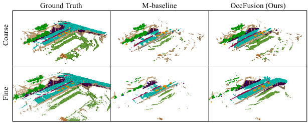
Figure 2: Comparison of our method with the existing SOTA multi-modal baseline [34] under challenging samples. The first row compares M-baseline [34] with our proposed OccFusion for the coarse occupancy prediction task, while the second row compares M-CONet [34] with our Active M-CONet. It is evident that our method achieves higher fidelity in scene detail reconstruction and stronger robustness. Better viewed when zoomed in.

2 Related Work

2.1 Vision-Based 3D Occupancy Prediction

Efficiently representing the 3D environment surrounding the ego-vehicle remains a core issue in autonomous driving. Voxel-based representation discretizes 3D space into a voxel grid, calculating features for each voxel to depict the scene. This method achieves finer-grained features than BEV (Bird’s Eye View) based methods [21, 24, 27, 39, 44], aligning more closely with real-world driving scenarios. The lack of direct geometric inputs and localization information [3] makes 3D occupancy prediction based solely on cameras challenging. MonoScene [4] is the first to predict occupancy using a single image. To address the limitations of a single camera, TPVFormer [14] employs a tri-perspective view representation for surrounding occupancy prediction, though resulting in sparse occupancy. Recent works have utilized depth prediction [34, 19, 4, 25, 43, 22] to generate occupancy features, but depth prediction is notoriously ill-posed, leading to instability in estimates. While camera-based methods hold promise, multi-modal approaches offer higher accuracy and reliability, which is crucial for the safe and trustworthy deployment of autonomous driving technologies.

2.2 Multi-modal 3D Occupancy Prediction

LiDAR provides accurate positional and reflectance information, which cameras lack. However, LiDAR point clouds are often sparse and vary greatly in density, and LiDAR cannot provide detailed semantic information such as color or object edges [24]. Although incorporating multiple sensors may entail higher costs, multi-modal semantic occupancy prediction methods [34] that combine the advantages of LiDAR and cameras outperform those based solely on either LiDAR or cameras. For instance, M-CONet [34] lifts 2D image features to 3D and achieves state-of-the-art accuracy on current benchmark through adaptive fusion with 3D LiDAR features. Nonetheless, existing multi-modal approaches still face challenges in multi-channel fusion, and current works [34] continue to rely on depth estimation for extracting image features, which is not an efficient method. In contrast, our novel fusion method directly integrates LiDAR features with image features on a point-to-point basis, circumventing depth estimation issues and achieving state-of-the-art results on current benchmark.

2.3 Active Learning Methods

One core principle of active learning is that information is not uniformly distributed across training samples (i.e., some samples may not provide sufficient information for the training process), and thus, random sampling for model training can potentially impair model accuracy [23]. Active learning approaches interactively request data annotations from human oracles to learn more from more significant data. Our study draws inspiration from this concept, but strictly speaking, the methods used herein do not constitute active learning, as they do not involve new annotations by human experts. This is partly because 3D occupancy annotation is an exceedingly laborious task [34, 36], and mainly because our aim is to enable the model to learn and predict autonomously and specifically, without the need for additional human intervention. Inspired by previous active learning research [11, 9, 17], which suggests that samples with higher entropy require extra attention, our Active M-CONet focuses on refining only the coarse voxels with the highest entropy. Moreover, during the training phase, we prioritize samples with greater uncertainty. Experiments demonstrate that our method possesses computational performance advantages, while also improving model accuracy and robustness.

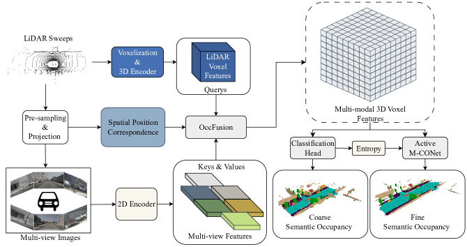
Figure 3: The overall architecture of our method. Raw LiDAR points are embedded and then processed by a 3D encoder to extract voxelized features as queries, while multi-view image features are directly obtained through a 2D encoder acting on surround-view images, serving as keys. LiDAR points, after pre-sampling (including sampling and generating), are projected onto images as reference points, establishing spatial position correspondence between LiDAR points and image features. The OccFusion module performs point-to-point fusion of 3D LiDAR voxel features and 2D image features to obtain multi-modal 3D voxel features. Coarse-grained prediction results are directly accessible through a classification head. Active M-CONet adaptively performs fine-grained prediction in more challenging areas.

3 Method

3.1 Overview

Figure 3 illustrates the architecture of our method. We employ VoxelNet [45] and 3D sparse convolutions [38] to embed raw LiDAR points into voxelized features $F^{L}\in R^{\frac{D}{S}\times\frac{H}{S}\times\frac{W}{S}\times C}$(where $S$ is the stride). For camera images, we use ResNet50 [10] as the backbone to extract multi-view features $F^{mv}\in R^{N\times H^{c}\times W^{c}\times C}$, without performing any depth-related operations. With the voxel grid established, the initial state’s point cloud is considered to reside within these voxels. Due to the sparsity of raw point clouds, to effectively sample image features, we employ specific sampling and generating methods (see Sec. 3.2) to ensure each voxel contains dense and relatively uniform LiDAR points. These LiDAR points are then projected onto images using camera intrinsic and extrinsic parameters, creating reference points. With LiDAR points as mediators, we establish the correspondence between LiDAR features and camera features. Through our proposed OccFusion module (see Sec. 3.3), we directly fuse 3D LiDAR features (as queries) and 2D image features (as keys) on a point-to-point basis. For each LiDAR point, we obtain a feature, and after averaging within each voxel, we derive a $C$ dimensional feature per voxel. These features can directly yield coarse occupancy predictions through a simple classification head. Due to the high computational complexity of directly predicting refined occupancy grids, we apply an Active Coarse to Fine Pipeline to our obtained coarse-grained multi-modal occupancy features, focusing fine-grained prediction only on voxels with the highest uncertainty (see Sec. 3.4). During the training phase, we experiment with enabling the model to actively learn from samples (see Sec. 3.5), which, as experiments shows (see Sec. 4.3), can further improve model accuracy.

3.2 3D LiDAR Feature Extraction and LiDAR Point Sampling Algorithm

The method for embedding raw LiDAR points into 3D voxelized features is consistent with [34]. In this process, 3D space is partitioned into a grid of size $D/S\times H/S\times W/S$ (where $S$ is the stride). After partitioning the space, the number of LiDAR points in voxel $V$ is denoted as $N_{p}^{V}$. We define two hyperparameters: $\tau\in\mathbb{N}$ and $\theta\in\mathbb{N}$ ($\theta>\tau$). For each voxel, there are three possible scenarios. First, due to the sparsity of LiDAR point clouds, many voxels contain no or few LiDAR points (i.e., $N_{p}^{V}\leq\tau$); for these, we generate synthetic point clouds using a simple equidistant uniform generation method to increase the point count to $\theta$. For voxels with an adequate number of LiDAR points (i.e., $\tau<N_{p}^{V}\leq\theta$), no action is taken. The uneven spatial distribution of LiDAR point clouds results in some voxels containing too many LiDAR points (i.e., $N_{p}^{V}>\theta$); for these, we use farthest point sampling (FPS) [29] to select $\theta$ points. Specifically, we start with a randomly chosen point $P_{0}$ as the initial point, forming a sample set $S=\{P_{0}\}$. We define the distance from a point $P$ to the set as $d(P,S):=\min d(P,P_{i}),P_{i}\in S$, calculate the distance $d(P_{j},S)$ for all points other than $P_{0}$, find

$$\alpha=\mathop{argmax}\limits_{j}{d(P_{j},S),P_{j}\notin S},$$ (1)

and add $P_{\alpha}$ to the set $S$, repeating this process until $\theta$ points are obtained. This point cloud sampling algorithm yields denser and more uniformly distributed point clouds in each voxel, facilitating effective sampling of image features.

Figure 4: Details of the OccFusion module. After pre-sampling, point clouds are projected onto images as reference points. Note that synthetic point clouds (points within circles) do not contribute to LiDAR feature generation. Due to overlapping fields of view among cameras, a single LiDAR point may correspond to multiple reference points upon projection. LiDAR points within the same voxel use the corresponding LiDAR feature of that voxel as the query, with image features serving as keys. Sampling is conducted near reference points through deformable attention [46], and the features corresponding to reference points are averaged to derive a feature for each LiDAR point, which are then averaged to obtain a multi-modal feature for a voxel. Multi-head attention is utilized but not shown in the figure for simplicity.

3.3 Camera Feature Extraction and OccFusion: Point-to-Point Multi-modal Feature Fusion

We utilize ResNet50 [10] as the 2D encoder to extract multi-view image features. Unlike previous multi-modal occupancy methods, we do not attempt to lift the spatial dimension of image features to 3D. Instead, we employ a novel OccFusion module to directly fuse 2D image features with 3D LiDAR features on a point-to-point basis. Specifically, we first project the pre-processed point clouds (see Sec. 3.2) onto multi-view images using camera intrinsic and extrinsic parameters, serving as reference points. Then, for a single LiDAR point, using the LiDAR voxel feature of the voxel where the LiDAR point is located as the query, we sample and fuse the corresponding image features using multi-head deformable attention [46] (since the fusion is primarily point-to-point, naive cross attention could also be utilized). Note that since the feature map dimensions are smaller than the original image, bilinear interpolation is used to obtain the sampling features at the corresponding positions. The mechanism of deformable attention and the process mentioned can be formalized as follows:

$$DeformAttn(z_{q},p_{q},x)=\sum_{m=1}^{N_{head}}W_{m}\sum_{k=1}^{N_{key}}A_{mqk}\cdot W_{m}^{{}^{\prime}}x(p_{q}+\Delta p_{mqk})$$ (2)

and

$$OccFuse(Q,X,V)=\frac{1}{\left|V\right|}\sum_{l\in{V}}\frac{1}{\left|\mathcal{P}_{L\rightarrow I}(l)\right|}\sum_{i\in\mathcal{P}_{L\rightarrow I}(l)}DeformAttn(Q_{V},i,X_{i}).$$ (3)

In this context, $Q$ represents the 3D LiDAR voxel features, and $X$ is the 2D feature map of surround-view images. The result on the left side of Eq. 3 corresponds to the final feature $F^{V}$ for a given voxel $V$, where $l$ is a LiDAR point within $V$, and $\mathcal{P}_{L\rightarrow I}(\cdot)$ denotes the projection from the LiDAR coordinate system to the image coordinate system. $\mathcal{P}_{L\rightarrow I}(l)$ is the set of reference points corresponding to the LiDAR point $l$ after projection. Notably, due to the shared field of view among cameras, a single LiDAR point may correspond to multiple reference points across several images upon projection (see Fig. 4). Moreover, a voxel always contains $|V|\in(\tau,\theta]$ LiDAR points after pre-sampling (see Sec. 3.2), where $|V|$ indicates the number of LiDAR points in voxel $V$, and $|\mathcal{P}_{L\rightarrow I}(l)|$ represents the number of reference points corresponding to a single LiDAR point $l$. We use averaging to handle these one-to-many relationships, ultimately obtaining a single feature vector $F^{V}$ for each voxel. $Q_{V}$ is the LiDAR feature corresponding to voxel $V$, and $X_{i}$ is the feature map of the image containing reference point $i$. $W_{m}$ and $W_{m}^{{}^{\prime}}$ are learnable parameters, $A_{mqk}$ denotes the attention weight, which is always 1 when the hyperparameter $N_{key}$ is set to 1. In the prediction phase, the derived feature $F^{V}$ is processed through a classification head, enabling direct coarse semantic occupancy prediction, see Fig. 4.

3.4 Active Coarse to Fine Pipeline

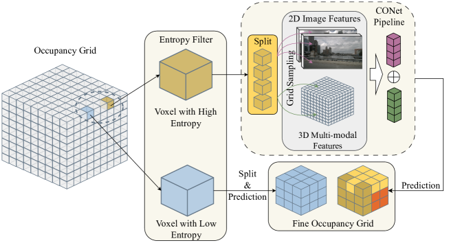
Figure 5: Active coarse to fine pipeline. We refine features only for voxels with greater uncertainty. For voxels with lower entropy, we directly use the coarse-grained prediction results but still split the voxel to achieve consistent granularity.

CONet (Cascade Occupancy Network) saves significant computational resources by refining coarse occupancy instead of directly predicting refined occupancy features [34]. However, we note that in real-world scenarios, it is not necessary to refine features for all voxels. For instance, for large objects like buses, a single voxel falling within the space occupied by the bus can sufficiently determine the category of that 3D space with a coarse-grained occupancy feature. Conversely, for very small objects such as traffic cones and bicycles, the coarse-grained occupancy grid is too sparse, making finer-grained prediction crucial. To conserve computational resources while optimizing the model’s ability to recognize small or intersecting objects, we introduce an entropy filter to actively determine whether each voxel requires feature refinement. Specifically, we employ classical information entropy to assess the need for fine-grained prediction in a voxel. We set a threshold $\delta$ representing the proportion of voxels requiring fine-grained feature prediction, and after passing coarse voxel features through a classification head, we obtain probabilities for each class in a voxel $V$ denoted as $p_{i}^{V},i=1,\ldots,N_{class}$, where $N_{class}$ is the total number of classes. Using the formula

$$\text{Entropy}(V)=-\sum_{i=1}^{N_{class}}p_{i}^{V}\log p_{i}^{V},$$ (4)

we calculate the uncertainty within each coarse-grained voxel. Note, the more uniform the predicted discrete distribution from the classification head, the higher this metric, indicating greater uncertainty. When $\text{Entropy}(V)$ is sufficiently high, we predict further fine-grained features for the voxel, i.e., splitting the voxel into smaller voxels to serve as occupancy queries for feature sampling through corresponding 2D image features and 3D multi-modal features using camera intrinsic and extrinsic parameters. The details are the same as the coarse to fine pipeline in [34]. For voxels with lower entropy, we still split them, but for each smaller voxel, we directly use the category obtained from coarse-grained features, see Fig. 5. Note that our pipeline can naturally be extended to other occupancy prediction models, not just multi-modal models.

3.5 Active Training Method

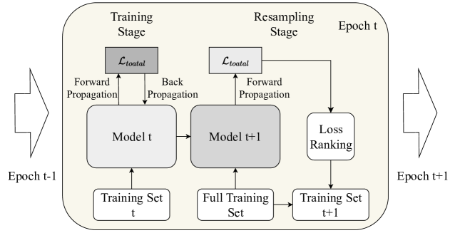
Figure 6: Active training method. A training epoch is divided into two stages. In the training stage, we train the model using the training set sampled from the previous stage. In the resampling stage, we use the model trained in the training stage to score the loss on the full training set, selecting the top K percent of samples to form the training set for the next training cycle.

In the dataset we utilize [34, 3], the complexity of different samples varies due to variations in the surrounding environment, affecting the difficulty level for the model to learn from these samples. Inspired by classic works in active learning [11, 9, 17], which rank training samples based on the model’s uncertainty in predictions and interact with human oracles to optimize the training process, we propose an active training strategy. Instead of optimizing 3D occupancy annotations manually, our model adaptively scores all samples at the end of each training epoch, allowing only the top K percent of scored samples to proceed to the next epoch of training (see Fig. 6). We use the model loss function directly as the scoring function. Our model loss is the sum of multiple loss functions, specifically, the cross-entropy loss $\mathcal{L}_{ce}$, lovasz-softmax $\mathcal{L}_{ls}$ [2], affinity loss $\mathcal{L}_{scal}^{geo}$ and $\mathcal{L}_{scal}^{sem}$ [4] (i.e., geometric IoU and semantic mIoU) are combined as the model’s loss function, formulated as:

$$\mathcal{L}_{total}=\mathcal{L}_{ce}+\mathcal{L}_{ls}+\mathcal{L}_{scal}^{geo}+\mathcal{L}_{scal}^{sem}.$$ (5)

Specifically, at epoch $t$, starting with the model trained in the previous epoch as model $t$, training is divided into two stages. In the training stage, we train using the training set $t$ filtered from the previous epoch to obtain model $t+1$. Then, using model $t+1$, we score the loss for each sample in the entire training set and rank these samples from high to low, see Fig. 6. The higher the loss for a sample, the greater the necessity for the model to re-learn that sample. Note, in the first round of training, we train the model using all samples. This active training method allows the model to learn from more challenging samples specifically. Although an additional resampling stage for loss ranking is required, this stage does not involve back-propagation, resulting in minimal computational overhead. Moreover, in each epoch (except the first), training only uses the top K percent of samples. Experiments show (see Tab. 3) that this approach significantly improves our model’s performance. Note that this simple yet effective training method can naturally be extended to other models or tasks in surrounding semantic perception.

4 Experiments

Table 1: Performance on the nuScenes-Occupancy validation set [34]. C, D, L, M represent camera, depth, LiDAR, and multi-modal, respectively. A-M-CONet stands for Active M-CONet, incorporating OccFusion and the active methods mentioned previously (see Figs. 5 and 6). Details of the baseline setup are available in the dataset [34].

Method	Input	IoU	mIoU	$\blacksquare$ barrier	$\blacksquare$ bicycle	$\blacksquare$ bus	$\blacksquare$ car	$\blacksquare$ const. veh.	$\blacksquare$ motorcycle	$\blacksquare$ pedestrian	$\blacksquare$ traffic cone	$\blacksquare$ trailer	$\blacksquare$ truck	$\blacksquare$ drive. suf.	$\blacksquare$ other flat	$\blacksquare$ sidewalk	$\blacksquare$ terrain	$\blacksquare$ manmade	$\blacksquare$ vegetation
MonoScene [4]	C	18.4	6.9	7.1	3.9	9.3	7.2	5.6	3.0	5.9	4.4	4.9	4.2	14.9	6.3	7.9	7.4	10.0	7.6
TPVFormer [14]	C	15.3	7.8	9.3	4.1	11.3	10.1	5.2	4.3	5.9	5.3	6.8	6.5	13.6	9.0	8.3	8.0	9.2	8.2
3DSketch [6]	C&D	25.6	10.7	12.0	5.1	10.7	12.4	6.5	4.0	5.0	6.3	8.0	7.2	21.8	14.8	13.0	11.8	12.0	21.2
AICNet [18]	C&D	23.8	10.6	11.5	4.0	11.8	12.3	5.1	3.8	6.2	6.0	8.2	7.5	24.1	13.0	12.8	11.5	11.6	20.2
LMSCNet [31]	L	27.3	11.5	12.4	4.2	12.8	12.1	6.2	4.7	6.2	6.3	8.8	7.2	24.2	12.3	16.6	14.1	13.9	22.2
JS3C-Net [37]	L	30.2	12.5	14.2	3.4	13.6	12.0	7.2	4.3	7.3	6.8	9.2	9.1	27.9	15.3	14.9	16.2	14.0	24.9
C-baseline [34]	C	19.3	10.3	9.9	6.8	11.2	11.5	6.3	8.4	8.6	4.3	4.2	9.9	22.0	15.8	14.1	13.5	7.3	10.2
L-baseline [34]	L	30.8	11.7	12.2	4.2	11.0	12.2	8.3	4.4	8.7	4.0	8.4	10.3	23.5	16.0	14.9	15.7	15.0	17.9
M-baseline [34]	C&L	29.1	15.1	14.3	12.0	15.2	14.9	13.7	15.0	13.1	9.0	10.0	14.5	23.2	17.5	16.1	17.2	15.3	19.5
OccFusion (ours)	C&L	31.1	17.0	15.9	15.1	15.8	18.2	15.0	17.8	17.0	10.4	10.5	15.7	26.0	19.4	19.3	18.2	17.0	21.2
C-CONet [34]	C	20.1	12.8	13.2	8.1	15.4	17.2	6.3	11.2	10.0	8.3	4.7	12.1	31.4	18.8	18.7	16.3	4.8	8.2
L-CONet [34]	L	30.9	15.8	17.5	5.2	13.3	18.1	7.8	5.4	9.6	5.6	13.2	13.6	34.9	21.5	22.4	21.7	19.2	23.5
M-CONet [34]	C&L	29.5	20.1	23.3	13.3	21.2	24.3	15.3	15.9	18.0	13.3	15.3	20.7	33.2	21.0	22.5	21.5	19.6	23.2
A-M-CONet (ours)	C&L	32.1	22.0	24.8	15.7	22.4	24.8	16.2	22.3	24.0	15.7	15.9	22.1	34.8	22.0	24.1	23.0	21.0	23.9

4.1 Experimental Setup

4.1.1 Dataset

We conduct experiments on the challenging nuScenes-Occupancy [34, 3], the first benchmark for surrounding semantic occupancy perception. It includes 28130 training frames and 6019 validation frames, with 17 semantic labels. Following OpenOccupancy [34], the evaluation range for the X and Y axes is set to $[-51.2m,51.2m]$, and for the Z axis, it is set to $[-3m,5m]$. The voxel resolution is 0.2m, resulting in a final occupancy grid spatial scale of $40\times 512\times 512$.

4.1.2 Implementation Details

For fairness, we adopt a foundational setup largely similar to the baseline provided by the dataset [34]. Specifically, we utilize an ImageNet [7] pretrained ResNet50 [10] as the 2D encoder for images, with an input image size of $1600\times 900$. During the training phase, we employ the AdamW [16] optimizer, with weight decay and initial learning rate set to 0.01 and 2e-4, respectively. A cosine learning rate scheduler with linear warm-up in the first 500 iterations is leveraged. Image augmentation strategies follow those used in BEVDet [13]. In the point pre-sampling process, hyper-parameters $\theta$ and $\tau$ are set to 20 and 5, respectively. Our model is trained for 24 epochs on 8 A100 GPUs with a batch size of 8. Moreover, the effectiveness of the active training method proposed above (see Sec. 3.5) is tested separately (see Tab. 3).

4.1.3 Evaluation Metric

Evaluation is conducted within the evaluation range specified by dataset [34]. We use Intersection of Union (IoU) as the geometric metric, treating all occupied voxels as a single category and solely determining whether voxels are occupied:

$$IoU=\frac{{TP}_{o}}{{TP}_{o}+{FP}_{o}+{FN}_{o}},$$ (6)

where ${TP}_{o}$, ${FP}_{o}$, and ${FN}_{o}$ are the true positive, false positive, and false negative predictions for occupied voxels, respectively. Additionally, mIoU (mean IoU of each class) is calculated as a semantic metric:

$$mIoU=\frac{1}{N_{class}}\sum_{c=1}^{N_{class}}\frac{{TP}_{c}}{{TP}_{c}+{FP}_{c}+{FN}_{c}},$$ (7)

where ${TP}_{c}$, ${FP}_{c}$, and ${FN}_{c}$ represent the true positive, false positive, and false negative counts for a specific class, respectively. $N_{class}$ denotes the total number of classes, with the noise category excluded as per the nuScenes-Occupancy specifications [34].

4.2 3D Semantic Occupancy Prediction

We compare our method against 12 baselines on OpenOccupancy (MonoScene [4], TPVFormer [14], 3DSketch [6], AICNet [18], LMSCNet [31], JS3C-Net [37], C-baseline [34], L-baseline [34], M-baseline [34], and CONet [34]), see Tab. 1. Results indicate our method surpasses the state-of-the-art (SOTA) methods in all categories except vegetation. Specifically, our OccFusion model exceeds the C-baseline by 65% and the L-baseline by 45% in the mIoU metric, showcasing the high reliability of multi-modal approaches. In comparison with existing multi-modal methods, OccFusion outperforms the M-baseline by 13%, and Active M-CONet surpasss M-CONet by 9%, as shown in Tab. 2. Our method makes remarkable progress on small objects. Specifically, Active M-CONet increases accuracy by 40% for motorcycles, 33% for pedestrians, and 18% for bicycles and traffic cones. Note that our method also demonstrates superior computational complexity (see Tab. 2). Our point cloud pre-sampling and point-to-point feature fusion strategy, which does not estimate depth for camera features, enables more precise and robust fusion of LiDAR and camera features. The active strategy further aids the model in finely learning difficult areas for occupancy prediction, with the impact of each method discussed in the next section.

Table 2: Experiment on the computational efficiency. w/o indicates without the corresponding method, GPU Mem. represents the GPU memory consumption at training phase.

Methods	GPU Mem.	GFLOPs
M-CONet	24.0 GB	3066
w/o active coarse to fine	19.1 GB	1721
Active M-CONet	16.9 GB	1554

4.3 Ablation Study

We conduct comprehensive ablation studies to demonstrate the effectiveness of the various methods proposed in this paper. Notably, our model still outperforms existing baselines even after the removal of any active methods or point cloud sampling algorithms (see Tab. 3). The FPS algorithm [29] and points generation ensure we achieve uniform point clouds in each voxel, thereby effectively sampling camera features. The active training method allows the model to prioritize learning from more challenging samples. We note that by implementing the entropy filter, we reduce substantial computational load (see Tab. 2), with only a minor decrease in mIoU by 0.2 (see Tab. 3).

Table 3: Ablation study on the proposed methods. w/o indicates without the corresponding method.

Methods	mIoU
w/o farthest point sampling	21.6
w/o points generation	21.5
w/o active training method	21.0
w/o active coarse to fine	22.2
Active M-CONet	22.0

In our proposed active training method, the training resampling proportion significantly impacts the training effectiveness due to the long-tail effect of samples, where more challenging samples should be prioritized for learning. In contrast, the majority of simpler samples do not contribute much to model optimization but still consume computational resources. We highlight that by selecting only 50% of the training samples during the resampling stage (see Tab. 4), our model already surpasses existing SOTA methods [34] in mIoU. When using 70% of the training samples, our method achieves the best results. Note that this strategy can be transferred to any surrounding semantic perception model.

Table 4: Ablation study on the resampling proportion in the resampling stage of the active training method

Training resampling proportion (percent)	mIoU
30	19.6
50	21.5
70	22.0

After obtaining coarse occupancy predictions, we employ an active coarse to fine pipeline for refined results. Experiments show that feature refinement for all voxels yields the best result (see Tab. 5). But by selecting only 20% of the voxels for refinement, our model already surpasses existing methods (see Tabs. 5 and 1). By refining just 30% of the coarse-grained voxels, we achieves an mIoU close to that of full refinement. Due to the efficiency of our OccFusion module and the active coarse to fine strategy, our model reduces GFLOPs and GPU memory consumption during the training phase by 49% and 30%, respectively, saving substantial computational resources.

Table 5: Ablation study on the proportion of voxels refined in the active coarse to fine pipeline

Coarse to fine proportion (percent)	mIoU
10	17.5
20	20.9
30	22.0
100	22.2

5 Conclusion

In this paper, we introduce OccFusion, a depth estimation-free multi-modal fusion method that addresses the lack of robustness in previous depth estimation-based fusion methods. Additionally, we propose an accompanying point cloud sampling algorithm for improved image feature sampling. An active coarse to fine pipeline is developed to adaptively learn more challenging areas within a sample while significantly reducing the computational load of fine-grained 3D occupancy prediction. Furthermore, we present an active training method that enhances the model’s training efficiency. Experiments conducted on OpenOccupancy demonstrate our method’s comprehensive superiority over existing state-of-the-art models, with ablation studies further illustrating the effectiveness of our proposed components.

References

- [1] Behley, J., Garbade, M., Milioto, A., Quenzel, J., Behnke, S., Stachniss, C., Gall, J.: Semantickitti: A dataset for semantic scene understanding of lidar sequences. In: ICCV. pp. 9297–9307 (2019). https://doi.org/10.1109/ICCV.2019.00939
- [2] Berman, M., Triki, A.R., Blaschko, M.B.: The lovasz-softmax loss: A tractable surrogate for the optimization of the intersection-over-union measure in neural networks. In: CVPR. pp. 4413–4421 (2018). https://doi.org/10.1109/CVPR.2018.00464
- [3] Caesar, H., Bankiti, V., Lang, A.H., Vora, S., Liong, V.E., Xu, Q., Krishnan, A., Pan, Y., Baldan, G., Beijbom, O.: nuscenes: A multimodal dataset for autonomous driving. In: CVPR. pp. 11618–11628 (2020). https://doi.org/10.1109/CVPR42600.2020.01164
- [4] Cao, A., de Charette, R.: Monoscene: Monocular 3d semantic scene completion. In: CVPR. pp. 3981–3991 (2022). https://doi.org/10.1109/CVPR52688.2022.00396
- [5] Chang, M.F., Lambert, J., Sangkloy, P., Singh, J., Bak, S., Hartnett, A., Wang, D., Carr, P., Lucey, S., Ramanan, D., Hays, J.: Argoverse: 3d tracking and forecasting with rich maps. In: CVPR. pp. 8748–8757 (2019). https://doi.org/10.1109/CVPR.2019.00895
- [6] Chen, X., Lin, K., Qian, C., Zeng, G., Li, H.: 3d sketch-aware semantic scene completion via semi-supervised structure prior. In: CVPR. pp. 4192–4201 (2020). https://doi.org/10.1109/CVPR42600.2020.00425
- [7] Deng, J., Dong, W., Socher, R., Li, L.J., Li, K., Fei-Fei, L.: Imagenet: A large-scale hierarchical image database. In: CVPR. pp. 248–255 (2009). https://doi.org/10.1109/CVPR.2009.5206848
- [8] Firman, M., Aodha, O.M., Julier, S., Brostow, G.J.: Structured prediction of unobserved voxels from a single depth image. In: CVPR. pp. 5431–5440 (2016). https://doi.org/10.1109/CVPR.2016.586
- [9] Gal, Y., Islam, R., Ghahramani, Z.: Deep bayesian active learning with image data. In: ICML. pp. 1183–1192 (2017)
- [10] He, K., Zhang, X., Ren, S., Sun, J.: Deep residual learning for image recognition. In: CVPR. pp. 770–778 (2016). https://doi.org/10.1109/CVPR.2016.90
- [11] Houlsby, N., Huszar, F., Ghahramani, Z., Lengyel, M.: Bayesian active learning for classification and preference learning. aeXiv preprint arXiv:1112.5745 (2011)
- [12] Hua, B.S., Pham, Q.H., Nguyen, D.T., Tran, M.K., Yu, L.F., Yeung, S.K.: Scenenn: A scene meshes dataset with annotations. In: 3DV. pp. 92–101 (2016). https://doi.org/10.1109/3DV.2016.18
- [13] Huang, J., Huang, G., Zhu, Z., Du, D.: Bevdet: High-performance multi-camera 3d object detection in bird-eye-view. aeXiv preprint arXiv:2112.11790 (2021)
- [14] Huang, Y., Zheng, W., Zhang, Y., Zhou, J., Lu, J.: Tri-perspective view for vision-based 3d semantic occupancy prediction. In: CVPR. pp. 9223–9232 (2023). https://doi.org/10.1109/CVPR52729.2023.00890
- [15] Kim, J., Choi, J., Kim, Y., Koh, J., Chung, C.C., Choi, J.W.: Robust camera lidar sensor fusion via deep gated information fusion network. In: IV. pp. 1620–1625 (2018). https://doi.org/10.1109/IVS.2018.8500711
- [16] Kingma, D.P., Ba, J.: Adam: A method for stochastic optimization. In: ICLR (2015)
- [17] Kirsch, A., van Amersfoort, J., Gal, Y.: Batchbald: Efficient and diverse batch acquisition for deep bayesian active learning. In: NeurIPS. pp. 7024–7035 (2019)
- [18] Li, J., Han, K., Wang, P., Liu, Y., Yuan, X.: Anisotropic convolutional networks for 3d semantic scene completion. In: CVPR. pp. 3348–3356 (2020). https://doi.org/10.1109/CVPR42600.2020.00341
- [19] Li, Y., Yu, Z., Choy, C.B., Xiao, C., Álvarez, J.M., Fidler, S., Feng, C., Anandkumar, A.: Voxformer: Sparse voxel transformer for camera-based 3d semantic scene completion. In: CVPR. pp. 9087–9098 (2023). https://doi.org/10.1109/CVPR52729.2023.00877
- [20] Li, Y., Yu, A.W., Meng, T., Caine, B., Ngiam, J., Peng, D., Shen, J., Lu, Y., Zhou, D., Le, Q.V., Yuille, A.L., Ta, M.: Deepfusion: Lidar-camera deep fusion for multi-modal 3d object detection. In: CVPR. pp. 17161–17170 (2022). https://doi.org/10.1109/CVPR52688.2022.01667
- [21] Li, Z., Wang, W., Li, H., Xie, E., Sima, C., Lu, T., Yu, Q., Dai, J.: Bevformer: Learning bird’s-eye-view representation from multi-camera images via spatiotemporal transformers. In: ECCV. pp. 1–18 (2022). https://doi.org/10.1007/978-3-031-20077-9_1
- [22] Li, Z., Yu, Z., Austin, D., Fang, M., Lan, S., Kautz, J., Álvarez, J.M.: Fb-occ: 3d occupancy prediction based on forward-backward view transformation. aeXiv preprint arXIv:2307.01492 (2023). https://doi.org/10.48550/arXiv.2307.01492
- [23] Liu, P., Wang, L., Ranjan, R., He, G., Zhao, L.: A survey on active deep learning: From model driven to data driven. ACM Comput. Surv. 54(10s), 221:1–221:34 (2022). https://doi.org/10.1145/3510414
- [24] Liu, Y., Wang, T., Zhang, X., Sun, J.: Petr: Position embedding transformation for multi-view 3d object detection. In: ECCV. pp. 531–548 (2022). https://doi.org/10.1007/978-3-031-19812-0_31
- [25] Miao, R., Liu, W., Chen, M., Gong, Z., Xu, W., Hu, C., Zhou, S.: Occdepth: A depth-aware method for 3d semantic scene completion. arXiv preprint arXiv:2302.13540 (2023). https://doi.org/10.48550/arXiv.2302.13540
- [26] Min, C., Xiao, L., Zhao, D., Nie, Y., Dai, B.: Uniscene: Multi-camera unified pre-training via 3d scene reconstruction. arXiv preprint arXiv:2305.18829 (2023). https://doi.org/10.48550/arXiv.2305.18829
- [27] Philion, J., Fidler, S.: Lift, splat, shoot: Encoding images from arbitrary camera rigs by implicitly unprojecting to 3d. In: ECCV. pp. 194–210 (2020). https://doi.org/10.1007/978-3-030-58568-6_12
- [28] Qi, C.R., Zhou, Y., Najibi, M., Sun, P., Vo, K., Deng, B., Anguelov, D.: Offboard 3d object detection from point cloud sequences. In: CVPR. pp. 6134–6144 (2021). https://doi.org/10.1109/CVPR46437.2021.00607
- [29] Qi, C.R., Yi, L., Su, H., Guibas, L.J.: Pointnet++: Deep hierarchical feature learning on point sets in a metric space. In: NeurIPS. pp. 5099–5108 (2017)
- [30] Reading, C., Harakeh, A., Chae, J., Waslander, S.L.: Categorical depth distribution network for monocular 3d object detection. In: CVPR. pp. 8555–8564 (2021). https://doi.org/10.1109/CVPR46437.2021.00845
- [31] Roldão, L., de Charette, R., Verroust-Blondet, A.: Lmscnet: Lightweight multiscale 3d semantic completion. In: 3DV. pp. 111–119 (2020). https://doi.org/10.1109/3DV50981.2020.00021
- [32] Vobecky, A., Siméoni, O., Hurych, D., Gidaris, S., Bursuc, A., Pérez, P., Sivic, J.: Pop-3d: Open-vocabulary 3d occupancy prediction from images. arXiv preprint arXiv:2401.09413 (2024). https://doi.org/10.48550/arXiv.2401.09413
- [33] Vora, S., Lang, A.H., Helou, B., Beijbom, O.: Pointpainting: Sequential fusion for 3d object detection. In: CVPR. pp. 4603–4611 (2020). https://doi.org/10.1109/CVPR42600.2020.00466
- [34] Wang, X., Zhu, Z., Xu, W., Zhang, Y., Wei, Y., Chi, X., Ye, Y., Du, D., Lu, J., Wang, X.: Openoccupancy: A large scale benchmark for surrounding semantic occupancy perception. In: ICCV. pp. 17804–17813 (2023). https://doi.org/10.1109/ICCV51070.2023.01636
- [35] Wang, Y., Chao, W.L., Garg, D., Hariharan, B., Campbell, M., Weinberger, K.Q.: Pseudo-lidar from visual depth estimation: Bridging the gap in 3d object detection for autonomous driving. In: CVPR. pp. 8445–8453 (2019). https://doi.org/10.1109/CVPR.2019.00864
- [36] Wei, Y., Zhao, L., Zheng, W., Zhu, Z., Zhou, J., Lu, J.: Surroundocc: Multi-camera 3d occupancy prediction for autonomous driving. In: ICCV. pp. 21672–21683 (2023). https://doi.org/10.1109/ICCV51070.2023.01986
- [37] Yan, X., Gao, J., Li, J., Zhang, R., Li, Z., Huang, R., Cui, S.: Sparse single sweep lidar point cloud segmentation via learning contextual shape priors from scene completion. In: AAAI. pp. 3101–3109 (2021). https://doi.org/10.1609/AAAI.V35I4.16419
- [38] Yan, Y., Mao, Y., Li, B.: Second: Sparsely embedded convolutional detection. Sensors 18(10) (2018). https://doi.org/10.3390/S18103337
- [39] Yang, C., Chen, Y., Tian, H., Tao, C., Zhu, X., Zhang, Z., Huang, G., Li, H., Qiao, Y., Lu, L., Zhou, J., Dai, J.: Bevformer v2: Adapting modern image backbones to bird’s-eye-view recognition via perspective supervision. In: CVPR. pp. 17830–17839 (2023). https://doi.org/10.1109/CVPR52729.2023.01710
- [40] Yin, T., Zhou, X., Krähenbühl, P.: Multimodal virtual point 3d detection. In: NeurIPS. pp. 16494–16507 (2021)
- [41] Zhang, C., Yan, J., Wei, Y., Li, J., Liu, L., Tang, Y., Duan, Y., Lu, J.: Occnerf: Self-supervised multi-camera occupancy prediction with neural radiance fields. arXiv preprint arXiv:2312.09243 (2023). https://doi.org/10.48550/arXiv.2312.09243
- [42] Zhang, Y., Zheng, W., Zhu, Z., Huang, G., Lu, J., Zhou, J.: A simple baseline for multi-camera 3d object detection. In: AAAI. pp. 3507–3515 (2023). https://doi.org/10.1609/aaai.v37i3.25460
- [43] Zhang, Y., Zhu, Z., Du, D.: Occformer: Dual-path transformer for vision-based 3d semantic occupancy prediction. In: ICCV. pp. 9399–9409 (2023). https://doi.org/10.1109/ICCV51070.2023.00865
- [44] Zhou, B., Krähenbühl, P.: Cross-view transformers for real-time map-view semantic segmentation. In: CVPR. pp. 13750–13759 (2022). https://doi.org/10.1109/CVPR52688.2022.01339
- [45] Zhou, Y., Tuzel, O.: Voxelnet: End-to-end learning for point cloud based 3d object detection. In: CVPR. pp. 4490–4499 (2018). https://doi.org/10.1109/CVPR.2018.00472
- [46] Zhu, X., Su, W., Lu, L., Li, B., Wang, X., Dai, J.: Deformable detr: Deformable transformers for end-to-end object detection. In: ICLR (2021)