DiffSF: Diffusion Models for Scene Flow Estimation

Abstract

Scene flow estimation is an essential ingredient for a variety of real-world applications, especially for autonomous agents, such as self-driving cars and robots. While recent scene flow estimation approaches achieve a reasonable accuracy, their applicability to real-world systems additionally benefits from a reliability measure. Aiming at improving accuracy while additionally providing an estimate for uncertainty, we propose DiffSF that combines transformer-based scene flow estimation with denoising diffusion models. In the diffusion process, the ground truth scene flow vector field is gradually perturbed by adding Gaussian noise. In the reverse process, starting from randomly sampled Gaussian noise, the scene flow vector field prediction is recovered by conditioning on a source and a target point cloud. We show that the diffusion process greatly increases the robustness of predictions compared to prior approaches resulting in state-of-the-art performance on standard scene flow estimation benchmarks. Moreover, by sampling multiple times with different initial states, the denoising process predicts multiple hypotheses, which enables measuring the output uncertainty, allowing our approach to detect a majority of the inaccurate predictions. The code is available at https://github.com/ZhangYushan3/DiffSF.

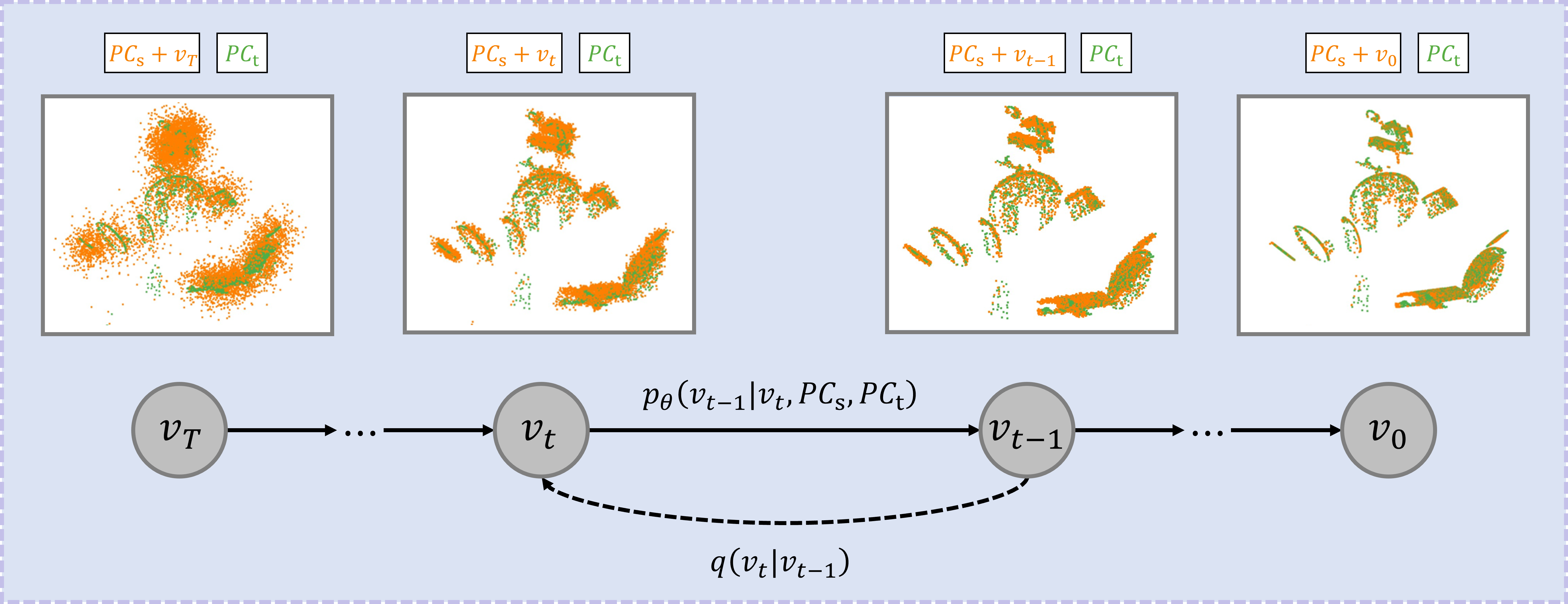
Figure 1: Diffusion process. In the forward process, we start from a ground truth scene flow vector field $v_{0}$ and gradually add noise to it until we reach $v_{T}$, which is completely Gaussian noise. In the reverse process, we recover the scene flow vector field $v_{0}$ from the randomly sampled noisy vector field $v_{T}$ conditioned on the source point cloud $PC_{\mathrm{s}}$ and the target point cloud $PC_{\mathrm{t}}$.

1 Introduction

Scene flow estimation is an important research topic in computer vision with applications in various fields, such as autonomous driving [39], and robotics [46]. Given a source and a target point cloud, the objective is to estimate a scene flow vector field that maps each point in the source point cloud to the target point cloud. Many studies on scene flow estimation aim at enhancing accuracy and substantial progress has been made particularly on clean, synthetic datasets. However, real-world data contains additional challenges such as severe occlusion and noisy input, thus requiring a high level of robustness when constructing models for scene flow estimation.

Recently, Denoising Diffusion Probabilistic Models (DDPMs) have not only been widely explored in image generation [19, 44], but also in analysis tasks, e.g. detection [5], classification [18], segmentation [2, 17], optical flow [45], human pose estimation [20], point cloud registration [23], etc. Drawing inspiration from the recent successes of diffusion models in regression tasks and recognizing their potential compatibility with scene flow estimation, we formulate scene flow estimation as a diffusion process following DDPMs [19] as shown in Figure 1. The forward process initiates from the ground truth scene flow vector field and gradually introduces noise to it. Conversely, the reverse process is conditioned on the source and the target point cloud and is tasked to reconstruct the scene flow vector field based on the current noisy input. To learn the denoising process, a new network is proposed inspired by state-of-the-art scene flow estimation methods FLOT [42] and GMSF [66].

Previous methods [66, 7, 57, 6] usually suffer from inaccuracies when occlusions occur or when dealing with noisy inputs. During inference, based on the fixed parameters learned during training, they cannot provide any information about their inaccurate predictions, which might lead to problems in safety-critical downstream tasks. Our proposed method approaches this problem in two aspects: First, denoising diffusion models are capable of handling noisy data by modeling stochastic processes. The noise caused by sensors in the real world is filtered out which allows the model to focus on learning underlying patterns. By learning feature representations that are robust to noise, the prediction accuracy is improved. Second, since the diffusion process introduces randomness into the inherently deterministic prediction task, it can provide a measure of uncertainty for each prediction by averaging over a set of hypotheses, notably without any modifications to the training process.

Extensive experiments on multiple scene flow estimation benchmarks FlyingThings3D [37], KITTI [39], and Waymo-Open [51] demonstrate state-of-the-art performance of our proposed method. Furthermore, we demonstrate that the predicted uncertainty correlates with the prediction error, establishing it as a reasonable measure that can be adjusted to the desired certainty level with a simple threshold value. Summarizing, our contributions are:

• We introduce DiffSF, leveraging diffusion models to solve the full scene flow estimation problem, where the inherent noisy property of the diffusion process filters out noisy data, thus, increasing the focus on learning the relevant patterns.

• DiffSF introduces randomness to the scene flow estimation task, which allows us to predict the uncertainty of the estimates without being explicitly trained for this purpose.

• We develop a novel architecture that combines transformers and diffusion models for the task of scene flow estimation, improving both accuracy and robustness for a variety of datasets.

2 Related Work

Scene Flow Estimation has rapidly progressed since the introduction of KITTI Scene Flow [39], FlyingThings3D [37], and Waymo-Open [51] benchmarks. Many existing methods [4, 36, 39, 43, 48, 56, 65] assume scene objects are rigid and break down the estimation task into sub-tasks involving object detection or segmentation, followed by motion model fitting. While effective for autonomous driving scenes with static backgrounds and moving vehicles, these methods struggle with more complex scenes containing deformable objects, and their non-differentiable components impede end-to-end training without instance-level supervision.

Recent advancements in scene flow estimation draw inspirations from optical flow tasks [11, 22, 50, 52], and are categorized into encoder-decoder, coarse-to-fine, recurrent, and soft correspondence methods. Encoder-decoder techniques, exemplified by FlowNet3D [35, 61] and HPLFlowNet [16], utilize neural networks to learn scene flow by adopting an hourglass architecture. Coarse-to-fine methods, such as PointPWC-Net [64], progressively estimate motion from coarse to fine scales, leveraging hierarchical feature extraction and warping. Recurrent methods like FlowStep3D [27], PV-RAFT [62], and RAFT3D [53] iteratively refine the estimated motion, thus enhancing accuracy. Some approaches FLOT [42], STCN[29], and GMSF [66] frame scene flow estimation as an optimal transport problem, employing convolutional layers and point transformer modules for correspondence computation.

Some works focus on bidirectional learning architectures. Bi-PointFlow [6] proposes a bidirectional learning architecture, where features are learned from both forward and backward directions. MSBRN [7] based on the multi-scale bidirectional learning architecture, further proposes a recurrent architecture that can iteratively refine the point features. DifFlow3D [34] introduces diffusion models for scene flow estimation refinement that can serve as a plug-in module to existing works. While this approach also employs diffusion models, it uses them solely for the purpose of refining an initial scene flow estimation. To train the refinement module, the ground truth residual scene flow has to be predetermined based on the initial estimation. By contrast, our approach aims to solve the scene flow problem in a single step without relying on error-prone preprocessing. Moreover, DifFlow3D is based on Gated Recurrent Units (GRU) while ours relies on a more advanced transformer architecture.

Other work such as 3DFlow [57] investigates the important building blocks of scene flow estimation approaches, such as point similarity calculation, scene flow predictor, and flow refinement level. PointConvFormer [63] introduced a novel building block for point cloud based deep network architectures, which works well for scene flow estimation. M-FUSE [38] breaks the limitation of estimating scene flow from two frame pairs and proposes to exploit temporal information by a novel multi-frame approach. DELFlow [40] regularizes 3D coordinates into dense 2D grids, enabling efficient learning on large-scale point clouds. FEAST [58] applies Spatial-Temporal Attention for scene flow estimation. A Spatial Abstraction layer and a Temporal Abstraction layer are proposed to help alleviate the instability caused by sparsity and irregularity in point clouds. IHNet [60] introduces a novel Iterative Hierarchical Network. The approach takes high-resolution estimated information back to the low-resolution layer serving as a guidance.

Furthermore, alternative strategies focus on runtime optimization [32, 28, 1, 33, 8], prior assumptions [41, 30, 31, 10, 55], and self-supervision [3, 54, 24, 47]. NSFP [32] first proposes runtime optimization with scene flow priors. SCOOP [28] combines runtime optimization with self-supervision for flow refinement. OptFlow [1] presents a fast runtime optimization-based method by improving the convergence speed of the optimization method. FNSF [33] focuses on speeding up NSFP by the rediscover distance transform as an efficient loss function and a replacement for Chamfer distance. Most recently, Chodosh et al. [8] achieve state-of-the-art performance in LiDAR scene flow estimation by combining Iterative Closest Point (ICP), rigid assumptions, and runtime optimization, obviating the need for training data. Pontes et al. [41] enforce scene flow rigidity using graph Laplacian constraints. HCRF-Flow [30] introduces high-order Conditional Random Fields to explore both point-wise smoothness and region-wise rigidity. RigidFlow [31] proposes a self-supervised learning approach with local rigidity priors. Dong et al. [10] explore rigidity constraints to preserve the geometric structure of the objects in the scenes. MBNSF [55] incorporates multi-body rigidity regularization into neural scene flow. Sac-flow [54] focuses on improving the necessary regularization for the task of scene flow estimation and introduces two new consistency losses, namely Surface Awareness loss and Cyclic Consistency loss. Gojcic et al. [14] reason the task at the object level and enable weakly-supervision. Shen et al. [47] introduce a new framework with a superpoint-guided flow refinement module. In contrast to the listed work, we propose to estimate the scene flow with a diffusion-based approach, which not only shows improved accuracy but also allows for uncertainty estimation.

Diffusion Models for Regression. Diffusion models as generative models have been exploited for image generation [19, 44]. Despite their ability to generate realistic images and videos, their ability to approach regression tasks has also been explored. CARD [18] introduces a classification and regression diffusion to accurately capture the mean and the uncertainty of the prediction. DiffusionDet [5] formulates object detection as a denoising diffusion process from noisy boxes to object boxes. Baranchuk et al. [2] employ diffusion models for semantic segmentation with scarce labeled data. DiffusionInst [17] depicts instances as instance-aware filters and casts instance segmentation as a denoising process from noise to filter. Jiang et al. [23] introduce diffusion models to point cloud registration that operates on the rigid body transformation group. Recent research on optical flow and depth estimation [45] shows that it is possible to use diffusion models as a simple and generic framework for dense vision tasks. While there have been attempts to employ diffusion models for scene flow estimation [34], they mainly focus on refining an initial estimation. On the other hand, our goal is to construct a model to estimate the full scene flow vector field instead of a refinement plug-in module. To the best of our knowledge, we are the first to apply a diffusion model successfully for the task of scene flow estimation.

Uncertainty of ML Models. Traditional deep learning methods typically provide point estimates of model parameters and predictions, without quantifying uncertainty. There are several ways to incorporate uncertainty into deep neural networks. Ensemble Learning [67] trains multiple deep neural networks separately and the predictions of different methods are combined to improve the results and indicate the uncertainty. Monte Carlo Dropout [13] extends dropout regularization to inference. Instead of using a single fixed forward pass to make predictions, Monte Carlo Dropout involves performing multiple inferences with dropout enabled. This introduces randomness to the process, resulting in uncertainty estimations. Bayesian Neural Networks (BNNs) [25], defined as stochastic artificial neural networks trained using Bayesian inference, introduce stochastic components into the neural networks. Either stochastic activation or stochastic weights are employed to simulate multiple possible models. Variational Inference [26] is an approach to approximate posterior distribution for probabilistic models, including Bayesian neural networks, latent variable models, and probabilistic graphical models. The training usually involves optimizing a variational objective. Some methods focus on making deep neural networks uncertainty aware. Eldesokey et al. [12] train a separate estimator for the confidence prediction for depth completion. Hu et al. [21] propose uncertainty-aware losses for zero-shot semantic segmentation. Recently diffusion models have shown their ability to model uncertainty in human pose estimation DiffPose [20], classification and regression CARD [18], and optical flow and depth estimation DDVM [45]. Our work employs denoising diffusion probabilistic models for scene flow estimation, where uncertainty estimation can be attained as a by-product of the random process introduced by diffusion models.

3 Proposed Method

In this section, we first give a general introduction of scene flow estimation and diffusion models in Section 3.1 followed by our proposed method in Section 3.2 and Section 3.3.

3.1 Preliminaries

Scene Flow Estimation. Given a source point cloud $PC_{\mathrm{source}}\in\mathbb{R}^{N_{1}\times 3}$ and a target point cloud $PC_{\mathrm{target}}\in\mathbb{R}^{N_{2}\times 3}$, where $N_{1}$ and $N_{2}$ are the number of points in the source and the target point cloud respectively, the objective is to estimate a scene flow vector field $V\in\mathbb{R}^{N_{1}\times 3}$ that maps each source point to the target.

There are two challenges in the scene flow estimation task. First, because of the sparse nature of the data, the points in the source and the target point cloud do not have a perfect one-to-one matching, even in the case when $N_{1}=N_{2}$. Second, occlusions commonly occur in real data. Estimating when certain parts of the source point cloud are not visible in the target point cloud, and vice versa, poses an additional challenge.

Diffusion Models. Inspired by non-equilibrium thermodynamics, diffusion models [19, 49] are a class of latent variable ($x_{1},...,x_{T}$) models of the form $p_{\theta}(x_{0})=\int p_{\theta}(x_{0:T})dx_{1:T}$, where the latent variables are of the same dimensionality as the input data $x_{0}$. The joint distribution $p_{\theta}(x_{0:T})$ is also called the reverse process

$$p_{\theta}(x_{0:T})=p_{\theta}(x_{T})\prod_{t=1}^{T}p_{\theta}(x_{t-1}|x_{t}),$$ (1)

where

$$p_{\theta}(x_{t-1}|x_{t})=\mathcal{N}(x_{t-1};\mu_{\theta}(x_{t},t),\Sigma_{\theta}(x_{t},t)).$$ (2)

The approximate posterior $q(x_{1:T}|x_{0})$ is called the forward process, which is fixed to a Markov chain that gradually adds noise according to a predefined noise scheduler $\beta_{1:T}$

$$q(x_{1:T}|x_{0})=\prod_{t=1}^{T}q(x_{t}|x_{t-1}),$$ (3)

where

$$q(x_{t}|x_{t-1})=\mathcal{N}(x_{t};\sqrt{1-\beta_{t}}x_{t-1},\beta_{t}\mathbf{I}).$$ (4)

The training is performed by minimizing a variational bound on negative log-likelihood

$$\begin{split}\mathbb{E}_{q}[-\log p_{\theta}(x_{0})]&\leq\mathbb{E}_{q}[-\log\tfrac{p_{\theta}(x_{0:T})}{q(x_{1:T}|x_{0})}]\\ &=\mathbb{E}_{q}[D_{KL}(q(x_{T}|x_{0})\|p(x_{T}))\\ &+\textstyle\sum_{t>1}D_{KL}(q(x_{t-1}|x_{t},x_{0})\|p_{\theta}(x_{t-1}|x_{t}))-\log p_{\theta}(x_{0}|x_{1})].\end{split}$$ (5)

3.2 Scene Flow Estimation as Diffusion Process

We formulate the scene flow estimation task as a conditional diffusion process that is illustrated in Figure 1.

The forward process starts from ground truth scene flow vector field $v_{0}$ and ends at purely Gaussian noise $v_{T}$ by gradually adding Gaussian noise to the input data as in Eq. (4). Given that $\beta_{t}$ is small, Eq. (4) can be rewritten as

$$q(v_{t}|v_{0})=\mathcal{N}(v_{t};\sqrt{\bar{\alpha}_{t}}v_{0},(1-\bar{\alpha}_{t})\mathbf{I}),$$ (6)

where $\bar{\alpha}_{t}:=\prod_{s=1}^{t}(1-\beta_{s})$.

The reverse process predicts the ground truth $v_{0}$ from noisy input $v_{t}$ conditioned on both the source point cloud $PC_{\mathrm{s}}$ and the target point cloud $PC_{\mathrm{t}}$,

$$p_{\theta}(v_{t-1}|v_{t},PC_{\mathrm{s}},PC_{\mathrm{t}})=\mathcal{N}(v_{t-1};\mu_{\theta}(v_{t},PC_{\mathrm{s}},PC_{\mathrm{t}}),\textbf{I}).$$ (7)

Since the forward process posterior $q(v_{t-1}|v_{t},v_{0})$ can be obtained by Bayes’ Rule

$$q(v_{t-1}|v_{t},v_{0})=\mathcal{N}(v_{t-1};\tilde{\mu}_{t}(v_{t},v_{0}),\tilde{\beta}_{t}\mathbf{I}),$$ (8)

where $\tilde{\mu}_{t}(v_{t},v_{0}):=\tfrac{\sqrt{\bar{\alpha}_{t-1}}\beta_{t}}{1-\bar{\alpha}_{t}}v_{0}+\tfrac{\sqrt{\alpha_{t}}(1-\bar{\alpha}_{t-1})}{1-\bar{\alpha}_{t}}v_{t}$, and $\tilde{\beta}_{t}:=\tfrac{1-\bar{\alpha}_{t-1}}{1-\bar{\alpha}_{t}}\beta_{t}$. Minimizing the variational bound in Eq. (5) breaks down to minizing the difference between $\tilde{\mu}_{t}(v_{t},v_{0})$ and $\mu_{\theta}(v_{t},PC_{\mathrm{s}},PC_{\mathrm{t}})$. Since $v_{t}$ is constructed from $v_{0}$ by a predefined fixed noise scheduler, the training objective is further simplified to

$$\mathcal{L}=\|f_{\theta}(v_{t},PC_{\mathrm{s}},PC_{\mathrm{t}})-v_{0}\|,$$ (9)

where $f_{\theta}$ is a deep neural network. The detailed architecture is presented in section 3.3.

During inference, starting from randomly sampled Gaussian noise $v_{T}$, $v_{0}$ is reconstructed with the model $f_{\theta}$ according to the reverse process in Eq. (7). The detailed training and sampling algorithms are given in Algorithm 1 and Algorithm 2.

1 repeat

2       $v_{0}\sim q(v_{0})$, $\epsilon\sim\mathcal{N}(\mathbf{0},\mathbf{I})$;

3       $t\sim\text{Uniform}(\{1,...,T\})$;

4       $v_{t}=\sqrt{\bar{\alpha}}v_{0}+\sqrt{1-\bar{\alpha}}\epsilon$;

5       estimate $\hat{v}_{\mathrm{pred}}=f_{\theta}(v_{t},PC_{\mathrm{s}},PC_{\mathrm{t}})$;

6       optimize loss: $\mathcal{L}_{t}=\text{loss}(\hat{v}_{\mathrm{pred}},v_{0})$;

7      

8until converged;

Algorithm 1 Training

1 $v_{T}\sim\mathcal{N}(\textbf{0},\textbf{I})$;

2 for $t=T,...,1$ do

3       estimate $\hat{v}_{\mathrm{pred}}=f_{\theta}(v_{t},PC_{\mathrm{s}},PC_{\mathrm{t}})$;

4       if $t>1$: $\textbf{z}\sim\mathcal{N}(\textbf{0},\textbf{I})$;

5       else: $\textbf{z}=\textbf{0}$;

6       $v_{t-1}=\tilde{\mu}_{t}(v_{t},\hat{v}_{\mathrm{pred}})+\textbf{z}$;

7      

8return $v_{0}$;

Algorithm 2 Sampling

3.3 Architecture

We follow FLOT [42] and formulate the scene flow estimation as an optimal transport problem with feature similarities as transport costs. This formulation requires to learn reliable transport costs, i.e. feature similarities. Thus, the problem is further decomposed into learning discriminative and reliable features. The currently most advanced scene flow estimation approach GMSF [66] shows that transformer-based architectures are capable of learning robust and reliable features for point clouds. To leverage this, we enhance the FLOT architecture by incorporating concepts from the GMSF approach for computing feature similarities. Subsequently, we integrate the proposed new architecture into each denoising block. The reverse process with the detailed architecture of denoising blocks is given in Figure 2. The architecture follows the recent work FLOT [42], RCP [15], FlowStep3D [27] and consists of an initial estimation and a final prediction. The building blocks: Feature Extraction, Global Correlation, and Local-Global-Cross Transformer are built up based on the state-of-the-art scene flow estimation approach, GMSF [66], which solves the scene flow estimation via global matching based on feature similarities between point pairs, and shows that a local-global-cross transformer architecture helps to extract reliable features.

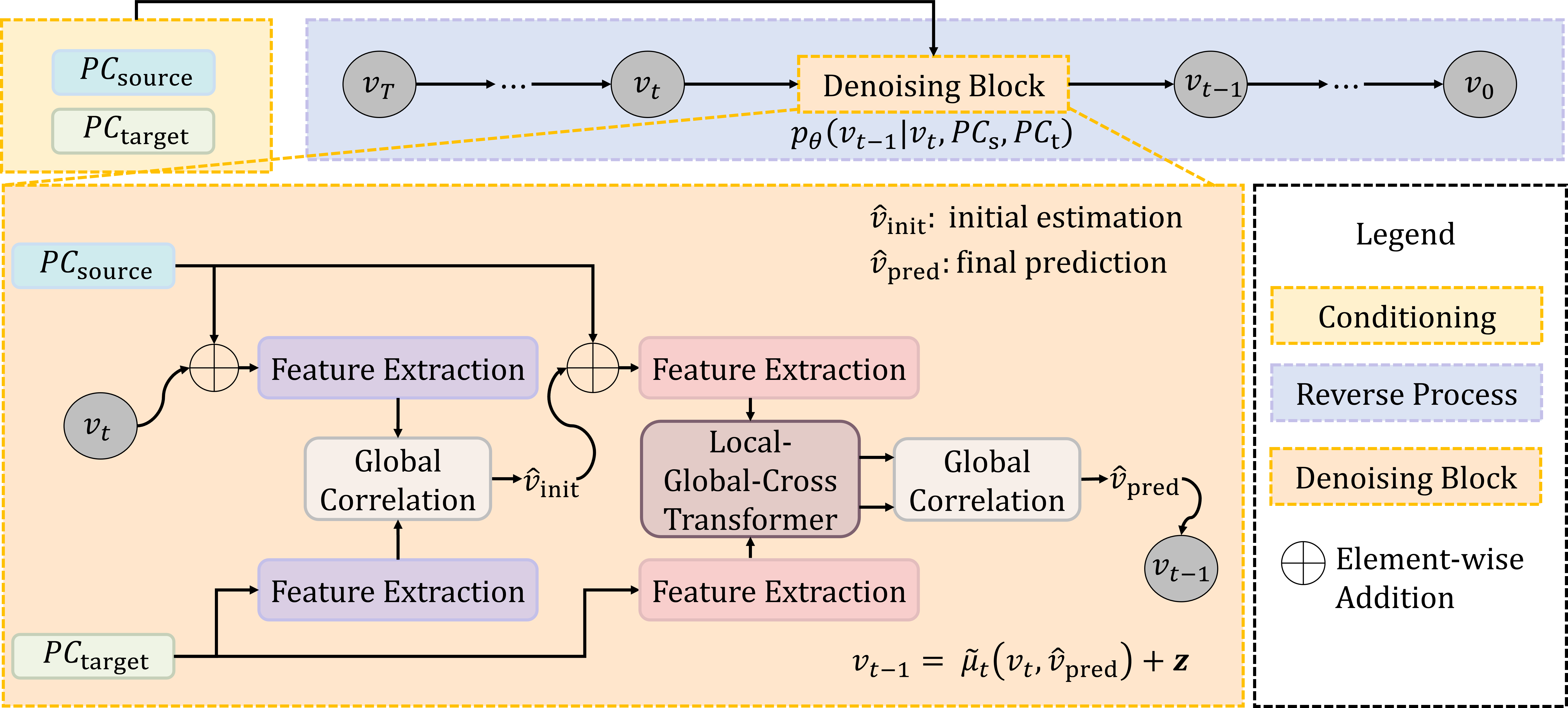
Figure 2: The reverse process with detailed denoising block for scene flow estimation. The denoising block takes the source point cloud $PC_{\text{source}}$ warped with the current noisy input $v_{t}$, and the target point cloud $PC_{\text{target}}$ as input. The output $\hat{v}_{\text{pred}}$ is the denoised scene flow prediction.

In the feature extraction stage, the three-dimensional coordinate is first projected into a higher feature dimension by the off-the-shelf feature extraction backbone DGCNN [59]

$$x_{i}^{h}=\max_{x_{j}\in\mathcal{N}(i)}h(x_{i},x_{j}-x_{i}),$$ (10)

where $i$ and $j$ denote the index of a single point in the point cloud. $\mathcal{N}(i)$ denotes the neighboring points of point $i$. $h$ represents a combination of linear layer, batch normalization, and non-linearity.

The high-dimensional features are then sent into a local-global-cross transformer to learn robust feature representations

$$x_{i}^{l}=\sum_{x_{j}\in\mathcal{N}(i)}\gamma(\varphi_{l}(x_{i}^{h})-\psi_{l}(x_{j}^{h})+\delta)\odot(\alpha_{l}(x_{j}^{h})+\delta),$$ (11)

$$x_{i}^{g}=\sum_{x_{j}\in\mathcal{X}_{1}}\langle\varphi_{g}(x_{i}^{l}),\psi_{g}(x_{j}^{l})\rangle\alpha_{g}(x_{j}^{l}),$$ (12)

$$x_{i}^{c}=\sum_{x_{j}\in\mathcal{X}_{2}}\langle\varphi_{c}(x_{i}^{g}),\psi_{c}(x_{j}^{g})\rangle\alpha_{c}(x_{j}^{g}),$$ (13)

where $\mathcal{X}_{1}$ and $\mathcal{X}_{2}$ represent the warped source point cloud (by $v_{t}$ or $\hat{v}_{\text{init}}$) and the target point cloud, respectively. $\gamma$ represents a multilayer perceptron. $\delta$ is the positional embedding. $\varphi$, $\psi$, and $\alpha$ denote linear projections to get the query, key, and value. The indices $\cdot_{l}$, $\cdot_{g}$, and $\cdot_{c}$ indicate local transformer, global transformer, and cross transformer, respectively. To acquire more robust feature representations, the global-cross transformers are stacked and repeated multiple times. For simplicity, we only give the equations for learning the features of $\mathcal{X}_{1}$. The features of $\mathcal{X}_{2}$ are computed by the same procedure. The output point features $x_{i}^{c}$ and $x_{j}^{c}$ for each point cloud are stacked together to form feature matrices $F_{1}$ and $F_{2}$.

In the global correlation stage, two feature similarity matrices are computed to guide the process

$$M_{\text{cross}}=\text{softmax}(F_{1}F_{2}^{T}/\sqrt{d}),$$ (14)

$$M_{\text{self}}=\text{softmax}(W_{q}(F_{1})W_{k}(F_{1})^{T}/\sqrt{d}),$$ (15)

where $W_{q}$ and $W_{k}$ are linear projections. $d$ is the feature dimensions. The global correlation is done by a probability approach guided by the cross feature similarity matrix followed by a smoothing procedure guided by the self feature similarity matrix

$$\hat{v}=M_{\text{self}}(M_{\text{cross}}PC_{\mathrm{target}}-PC_{\mathrm{source}}).$$ (16)

The loss employed is a robust loss defined as

$$\mathcal{L}=\sum_{i}(\lVert\hat{v}_{\text{pred}}(i)-v_{\text{gt}}(i)\rVert_{1}+\epsilon)^{q},$$ (17)

where $v_{\text{gt}}$ denotes the ground truth scene flow vector field. $i$ is the index of the points. $\epsilon$ is set to 0.01 and $q$ is set to 0.4.

4 Experiments

4.1 Implementation Details

Our method is implemented in Pytorch. We use AdamW optimizer and a weight decay of $1\times 10^{-4}$. The initial learning rate is set to $4\times 10^{-4}$ for FlyingThings3D and $1\times 10^{-4}$ for Waymo-Open. We employ learning rate annealing by using the Pytorch OneCycleLR learning rate scheduler. During training, we set $N_{1}$ and $N_{2}$ to $4096$. The model is trained for $600$k iterations with a batch size of $24$. During inference, we follow previous work and set $N_{1}$ and $N_{2}$ to $8192$.

4.2 Evaluation Metrics

We follow previous work and use standard evaluation metrics for scene flow estimation. $\textrm{EPE}_{\textrm{3D}}$ measures the end point error between the prediction and the ground truth $\lVert\hat{v}_{\mathrm{pred}}-v_{\mathrm{gt}}\rVert_{2}$ averaged over all the points. $\textrm{ACC}_{\textrm{S}}$ measures the percentage of the points that has an end point error smaller than $5~{}\textrm{cm}$ or relative error less than $5\%$. $\textrm{ACC}_{\textrm{R}}$ measures the percentage of the points that has an end point error smaller than $10~{}\textrm{cm}$ or relative error less than $10\%$. Outliers measures the percentage of the points that has an end point error larger than $30~{}\textrm{cm}$ or relative error larger than $10\%$.

4.3 Datasets

4.3.1 FlyingThings3D

is a synthetic dataset consisting of 25000 scenes with ground truth annotations. We follow Liu et al. in FlowNet3D [35] and Gu et al. in HPLFlowNet [16] to preprocess the dataset and denote them as $\text{F3D}_{\text{o}}$, with occlusions, and $\text{F3D}_{\text{s}}$, without occlusions. The former one consists of 20000 and 2000 scenes for training and testing respectively. The latter one consists of 19640 and 3824 scenes for training and testing respectively.

KITTI is a real autonomous driving dataset with 200 scenes for training and 200 scenes for testing. Since the annotated data in KITTI is limited, the dataset is mainly used for evaluating the generalization ability of the models trained on FlyingThings3D. Similar to the FlyingThings3D dataset, the KITTI dataset is preprocessed as $\text{KITTI}_{\text{o}}$, with occlusions, and $\text{KITTI}_{\text{s}}$, without occlusions. The former consists of 150 scenes from the annotated training set. The latter consists of 142 scenes from the annotated training set.

Waymo-Open is a larger autonomous driving dataset with challenging scenes [51]. The annotations are generated from corresponding tracked 3D objects to scale up the dataset for scene flow estimation by $\sim$1,000$\times$ compared to previous real-world scene flow estimation datasets. The dataset consists of 798 training sequences and 202 testing sequences. Each sequence consists of around 200 scenes. We follow [9, 66] to preprocess the dataset.

4.4 State-of-the-art Comparison

We give state-of-the-art comparisons on multiple standard scene flow datasets. Table 1 and Table 2 shows the results on the $\text{F3D}_{\text{s}}$ and the $\text{F3D}_{\text{o}}$ datasets, with generalization results on the $\text{KITTI}_{\text{s}}$ and the $\text{KITTI}_{\text{o}}$ datasets. Table 3 shows the results on the Waymo-Open dataset.

On the $\text{F3D}_{\text{s}}$ dataset, DiffSF achieves an EPE of $0.62~{}\textrm{cm}$, which shows an improvement of around $30$ percent compared to the current state-of-the-art method GMSF [66]. Similar improvement is also shown on the $\text{F3D}_{\text{o}}$ dataset, demonstrating DiffSF’s ability to handle occlusions. The generalization abilities on the $\text{KITTI}_{\text{s}}$ and the $\text{KITTI}_{\text{o}}$ datasets are comparable to state of the art. All the four metrics show the best or second-best performances. On the Waymo-Open dataset, a steady improvement in both accuracy and robustness is achieved, showing case DiffSF’s effectiveness on real-world data.

Table 1: State-of-the-art comparison on $\text{F3D}_{\text{s}}$ and $\text{KITTI}_{\text{s}}$. The models are only trained on $\text{F3D}_{\text{s}}$ prepared by [16] without occlusions. Testing results on $\text{F3D}_{\text{s}}$ and $\text{KITTI}_{\text{s}}$ are given. The number of time steps is set to 20 for training and 2 for inference.

Method	$\text{F3D}_{\text{s}}$				$\text{KITTI}_{\text{s}}$
	$\text{EPE}_{\text{3D}}\downarrow$	$\text{ACC}_{\text{S}}\uparrow$	$\text{ACC}_{\text{R}}\uparrow$	$\text{Outliers}\downarrow$	$\text{EPE}_{\text{3D}}\downarrow$	$\text{ACC}_{\text{S}}\uparrow$	$\text{ACC}_{\text{R}}\uparrow$	$\text{Outliers}\downarrow$
FlowNet3D [35]	0.1136	41.25	77.06	60.16	0.1767	37.38	66.77	52.71
HPLFlowNet [16]	0.0804	61.44	85.55	42.87	0.1169	47.83	77.76	41.03
PointPWC [64]	0.0588	73.79	92.76	34.24	0.0694	72.81	88.84	26.48
FLOT [42]	0.0520	73.20	92.70	35.70	0.0560	75.50	90.80	24.20
Bi-PointFlow [6]	0.0280	91.80	97.80	14.30	0.0300	92.00	96.00	14.10
3DFlow [57]	0.0281	92.90	98.17	14.58	0.0309	90.47	95.80	16.12
MSBRN [7]	0.0150	97.30	99.20	5.60	0.0110	97.10	98.90	8.50
DifFlow3D [34]	0.0140	97.76	99.33	4.79	0.0089	98.13	99.30	8.25
GMSF [66]	0.0090	99.18	99.69	2.55	0.0215	96.22	98.25	9.84
DiffSF(ours)	0.0062	99.54	99.80	1.41	0.0098	98.59	99.44	8.31

Table 2: State-of-the-art comparison on $\text{F3D}_{\text{o}}$ and $\text{KITTI}_{\text{o}}$. The models are only trained on $\text{F3D}_{\text{o}}$ prepared by [35] with occlusions. Testing results on $\text{F3D}_{\text{o}}$ and $\text{KITTI}_{\text{o}}$ are given. The number of time steps is set to 20 for training and 2 for inference.

Method	$\text{F3D}_{\text{o}}$				$\text{KITTI}_{\text{o}}$
	$\text{EPE}_{\text{3D}}\downarrow$	$\text{ACC}_{\text{S}}\uparrow$	$\text{ACC}_{\text{R}}\uparrow$	$\text{Outliers}\downarrow$	$\text{EPE}_{\text{3D}}\downarrow$	$\text{ACC}_{\text{S}}\uparrow$	$\text{ACC}_{\text{R}}\uparrow$	$\text{Outliers}\downarrow$
FlowNet3D [35]	0.157	22.8	58.2	80.4	0.183	9.8	39.4	79.9
HPLFlowNet [16]	0.168	26.2	57.4	81.2	0.343	10.3	38.6	81.4
PointPWC [64]	0.155	41.6	69.9	63.8	0.118	40.3	75.7	49.6
FLOT [42]	0.153	39.6	66.0	66.2	0.130	27.8	66.7	52.9
Bi-PointFlow [6]	0.073	79.1	89.6	27.4	0.065	76.9	90.6	26.4
3DFlow [57]	0.063	79.1	90.9	27.9	0.073	81.9	89.0	26.1
MSBRN [7]	0.053	83.6	92.6	23.1	0.044	87.3	95.0	20.8
DifFlow3D [34]	0.047	88.2	94.0	15.0	0.029	95.9	97.5	10.8
GMSF [66]	0.022	95.0	97.5	5.6	0.033	91.6	95.9	13.7
DiffSF(ours)	0.015	96.7	98.1	3.5	0.029	94.5	97.00	13.0

Table 3: State-of-the-art comparison on Waymo-Open dataset. The number of time steps is set to 20 for training and 2 for inference.

Method	$\text{EPE}_{\text{3D}}\downarrow$	$\text{ACC}_{\text{S}}\uparrow$	$\text{ACC}_{\text{R}}\uparrow$	$\text{Outliers}\downarrow$
FlowNet3D [35]	0.225	23.0	48.6	77.9
PointPWC [64]	0.307	10.3	23.1	78.6
FESTA [58]	0.223	24.5	27.2	76.5
FH-Net [9]	0.175	35.8	67.4	60.3
GMSF [66]	0.083	74.7	85.1	43.5
DiffSF(ours)	0.080	76.0	85.6	41.9

4.5 Uncertainty-error Correspondence

One of the key advantages of our proposed method DiffSF compared to other approaches is that DiffSF can model uncertainty during inference, without being explicitly trained for this purpose. We exploit the property of diffusion models to inject randomness into inherently deterministic tasks. Without having to train multiple models we predict multiple hypotheses using a single model with different initial randomly sampled noise.

Figure 3 shows that the standard deviation of several hypotheses for each point gives a reliable uncertainty estimation, which correlates very well with the inaccuracy of the prediction. Figure 3 (left) shows the relationship between the EPE and the standard deviation of the predictions averaged over the $\text{F3D}_{\text{o}}$ dataset. There is an almost linear correlation of the predicted uncertainty with the EPE underlining the usefulness of our uncertainty measure. Figure 3 (right) shows the recall and precision of the outlier prediction by the uncertainty. An outlier is defined as a point that has an EPE larger than 0.30 meters. The horizontal axis is the threshold applied to the uncertainty to determine the outliers. The recall is defined as the number of correctly retrieved outliers divided by the number of all the outliers. The precision is defined as the number of correctly retrieved outliers divided by the number of all the retrieved outliers. The precision-recall break-even point obtains around 55% of recall and 55% of precision.

Figure 3: Analysis of uncertainty estimation. Left: Uncertainty-error correspondences. The horizontal axis is an interval of EPE. The vertical axis is the estimated uncertainty averaged over all the points that fall in the interval and the indication of the scaled uncertainty standard deviation. Right: Recall and precision curve of outliers prediction. The horizontal axis is the threshold of the estimated uncertainty to determine the outliers. The two curves are the recall (red) and the precision (blue) curves.

Figure 4 shows visual examples that compare our outlier prediction with the actual outliers. The first row marks the scene flow estimation outliers with an EPE larger than 0.30 meters in red. The second row marks the outliers predicted by the uncertainty estimation in red. In summary, while every learned scene flow prediction model inevitably makes mistakes, our novel formulation of the task as a diffusion process not only produces state-of-the-art results but also allows for an accurate prediction of these errors. Moreover, our analysis shows that downstream tasks can select a threshold according to its desired precision and recall, therefore, mitigating potential negative effects that uncertain predictions might produce.

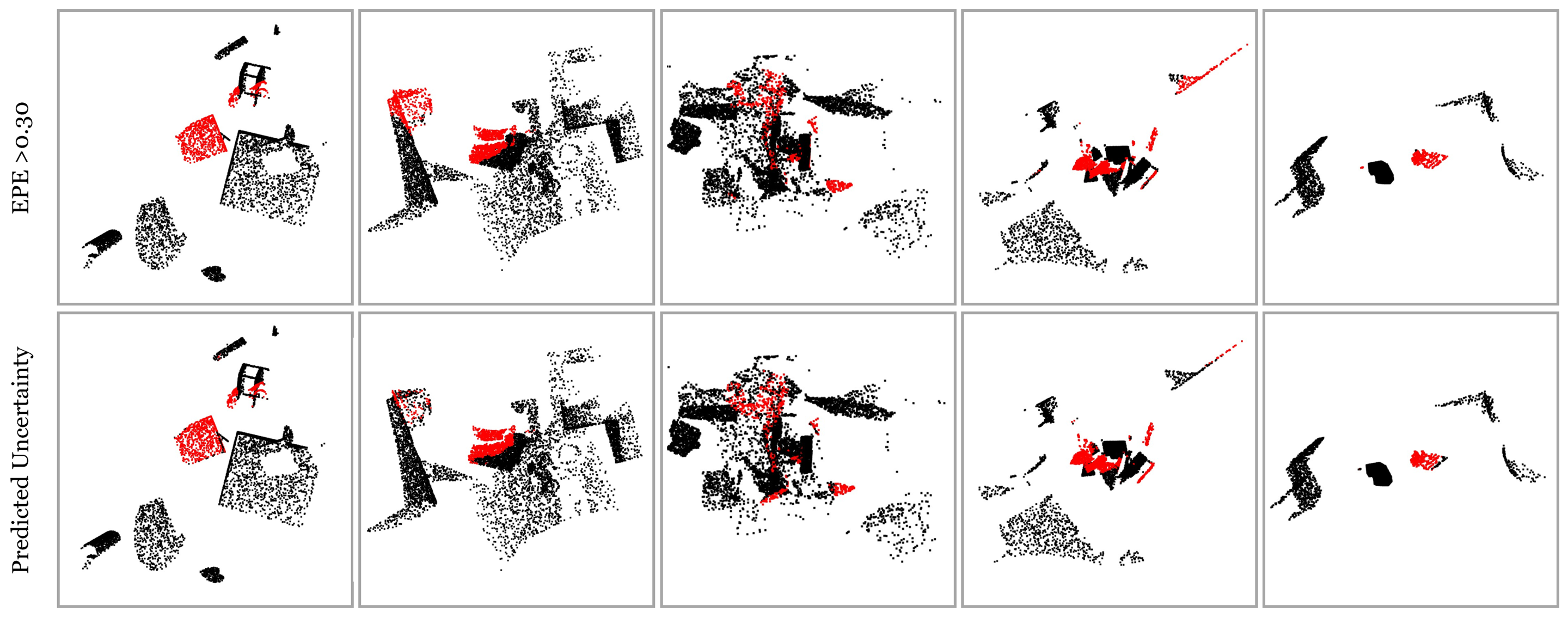
Figure 4: Visualization of outlier prediction. Black: Accurate prediction. Red: Outliers. Top row: Outliers defined as EPE > 0.30. Bottom row: Outliers predicted by Uncertainty.

4.6 Ablation Study

We investigate several key design choices of the proposed method. For the denoising model architecture, we investigate how the number of global-cross transformer layers and the number of feature channels have an impact on the results. For the diffusion process, we investigate the influence of the number of time steps for training and sampling.

Model Architecture. To evaluate different architectural choices we select a diffusion model with five denoising blocks during training and one denoising step during testing with the DDIM [49] sampling strategy. Table 4 shows the influence of the number of global-cross transformer layers on the results. The experiments show that the best performance is achieved at the number of $14$ layers. Table 5 shows the influence of the number of feature channels on the results. The experiments show that a smaller number of feature channels results in worse performance. The best performance is achieved at $128$ feature channels.

Number of Time Steps. We set the number of global-cross transformer layers as $14$ and the number of feature channels as $128$. We investigate the influence of different number of time steps during training and sampling on the results. The number of time steps investigated is $5$, $20$, and $100$ for training and $1$, $2$, $5$, and $20$ for sampling. The fast sampling is done by DDIM [49] instead of DDPM [19] sampling. Table 6 shows the results on the $\text{F3D}_{\text{o}}$ dataset, where $a@b$ denotes using $b$ training steps and $a$ sampling steps. While the results are very stable across a wide range of values the best performance is achieved at $2@20$ time steps. We hypothesize that compared to the standard setting of image generation, the lower dimensionality and variance of the scene flow data results in a smaller number of required time steps. For the number of time steps during inference, DDIM sampling works well with the best performance achieved at $2$ steps.

Table 4: Ablation study on the number of global-cross transformer layers on $\text{F3D}_{\text{o}}$. The number of time steps is set to $5$ for training and $1$ for inference.

Layers	$\text{EPE}_{\text{3D}}\downarrow$	$\text{ACC}_{\text{S}}\uparrow$	$\text{ACC}_{\text{R}}\uparrow$	$\text{Outliers}\downarrow$	$\text{EPE}_{\text{3D}}\downarrow$	$\text{ACC}_{\text{S}}\uparrow$	$\text{ACC}_{\text{R}}\uparrow$	$\text{Outliers}\downarrow$
	all				non-occ
8	0.0439	91.6	94.8	7.9	0.0205	95.2	97.5	5.1
10	0.0413	92.6	95.1	7.1	0.0189	95.8	97.6	4.5
12	0.0381	93.0	95.5	6.4	0.0168	96.1	97.8	3.9
14	0.0361	93.7	95.7	5.9	0.0153	96.5	98.0	3.5
16	0.0383	93.0	95.5	6.5	0.0168	96.1	97.8	4.0

Table 5: Ablation study on the number of feature channels on $\text{F3D}_{\text{o}}$. The number of time steps is set to $5$ for training and $1$ for inference.

Channels	$\text{EPE}_{\text{3D}}\downarrow$	$\text{ACC}_{\text{S}}\uparrow$	$\text{ACC}_{\text{R}}\uparrow$	$\text{Outliers}\downarrow$	$\text{EPE}_{\text{3D}}\downarrow$	$\text{ACC}_{\text{S}}\uparrow$	$\text{ACC}_{\text{R}}\uparrow$	$\text{Outliers}\downarrow$
	all				non-occ
32	0.0612	88.2	92.9	11.7	0.0299	92.9	96.3	8.2
64	0.0431	92.3	95.0	7.4	0.0199	95.7	97.5	4.7
128	0.0361	93.7	95.7	5.9	0.0153	96.5	98.0	3.5

Table 6: Ablation study on the number time steps for training and sampling on $\text{F3D}_{\text{o}}$. The number of global-cross transformer layers is set to $14$. The number of feature channels is set to $128$. $a@b$ denotes an inference of $b$ training steps and $a$ sampling steps.

Steps	$\text{EPE}_{\text{3D}}\downarrow$	$\text{ACC}_{\text{S}}\uparrow$	$\text{ACC}_{\text{R}}\uparrow$	$\text{Outliers}\downarrow$	$\text{EPE}_{\text{3D}}\downarrow$	$\text{ACC}_{\text{S}}\uparrow$	$\text{ACC}_{\text{R}}\uparrow$	$\text{Outliers}\downarrow$
	all				non-occ
1@5	3.609	93.700	95.729	5.898	1.527	96.548	97.971	3.520
2@5	3.591	93.713	95.721	5.903	1.519	96.554	97.956	3.535
5@5	3.592	93.716	95.719	5.907	1.521	96.557	97.954	3.539
1@20	3.588	93.867	95.912	5.796	1.504	96.728	98.080	3.517
2@20	3.576	93.866	95.921	5.788	1.491	96.732	98.085	3.507
5@20	3.580	93.861	95.919	5.787	1.492	96.727	98.086	3.504
20@20	3.580	93.859	95.915	5.792	1.492	96.725	98.083	3.507
1@100	3.678	93.503	95.665	6.016	1.587	96.376	97.844	3.689
2@100	3.663	93.545	95.662	6.010	1.579	96.398	97.838	3.697
5@100	3.668	93.546	95.663	6.010	1.583	96.400	97.842	3.695
20@100	3.670	93.545	95.663	6.015	1.584	96.396	97.843	3.700

5 Conclusions

We propose to estimate scene flow from point clouds using diffusion models in combination with transformers. Our novel approach improves significantly over the state-of-the-art in terms of both accuracy and robustness. Extensive experiments on multiple scene flow estimation benchmarks demonstrate the ability of DiffSF to handle both occlusions and real-world data. Furthermore, we propose to estimate uncertainty based on the randomness inherent in the diffusion process, which helps to indicate reliability for safety-critical downstream tasks. The proposed uncertainty estimation will enable mechanisms to mitigate the negative effects of potential failures.

Limitations. The training process of the diffusion models relies on annotated scene flow ground truth which is not easy to obtain for real-world data. Incorporating self-supervised training methods to leverage unannotated data might further improve our approach in the future. Furthermore, the transformer-based architecture and the global matching process require scaling the compute resources quadratically with the number of points. Consequently, if a large number of points is required, the architecture needs to be simplified.

Acknowledgements: This work was partly supported by the Wallenberg Artificial Intelligence, Autonomous Systems and Software Program (WASP), funded by Knut and Alice Wallenberg Foundation, and the Swedish Research Council grant 2022-04266; and by the strategic research environment ELLIIT funded by the Swedish government. The computational resources were provided by the National Academic Infrastructure for Supercomputing in Sweden (NAISS) partially funded by the Swedish Research Council grant 2022-06725, and by the Berzelius resource, provided by the Knut and Alice Wallenberg Foundation at the National Supercomputer Centre.

References

- [1] Ahuja, R., Baker, C., Schwarting, W.: Optflow: Fast optimization-based scene flow estimation without supervision. In: Proceedings of the IEEE/CVF Winter Conference on Applications of Computer Vision. pp. 3161–3170 (2024)
- [2] Baranchuk, D., Voynov, A., Rubachev, I., Khrulkov, V., Babenko, A.: Label-efficient semantic segmentation with diffusion models. In: International Conference on Learning Representations (2021)
- [3] Baur, S.A., Emmerichs, D.J., Moosmann, F., Pinggera, P., Ommer, B., Geiger, A.: Slim: Self-supervised lidar scene flow and motion segmentation. In: Proceedings of the IEEE/CVF International Conference on Computer Vision. pp. 13126–13136 (2021)
- [4] Behl, A., Hosseini Jafari, O., Karthik Mustikovela, S., Abu Alhaija, H., Rother, C., Geiger, A.: Bounding boxes, segmentations and object coordinates: How important is recognition for 3d scene flow estimation in autonomous driving scenarios? In: Proceedings of the IEEE International Conference on Computer Vision. pp. 2574–2583 (2017)
- [5] Chen, S., Sun, P., Song, Y., Luo, P.: Diffusiondet: Diffusion model for object detection. In: Proceedings of the IEEE/CVF International Conference on Computer Vision. pp. 19830–19843 (2023)
- [6] Cheng, W., Ko, J.H.: Bi-pointflownet: Bidirectional learning for point cloud based scene flow estimation. In: Computer Vision–ECCV 2022: 17th European Conference, Tel Aviv, Israel, October 23–27, 2022, Proceedings, Part XXVIII. pp. 108–124. Springer (2022)
- [7] Cheng, W., Ko, J.H.: Multi-scale bidirectional recurrent network with hybrid correlation for point cloud based scene flow estimation. In: Proceedings of the IEEE/CVF International Conference on Computer Vision. pp. 10041–10050 (2023)
- [8] Chodosh, N., Ramanan, D., Lucey, S.: Re-evaluating lidar scene flow for autonomous driving. arXiv preprint arXiv:2304.02150 (2023)
- [9] Ding, L., Dong, S., Xu, T., Xu, X., Wang, J., Li, J.: Fh-net: A fast hierarchical network for scene flow estimation on real-world point clouds. In: Computer Vision–ECCV 2022: 17th European Conference, Tel Aviv, Israel, October 23–27, 2022, Proceedings, Part XXXIX. pp. 213–229. Springer (2022)
- [10] Dong, G., Zhang, Y., Li, H., Sun, X., Xiong, Z.: Exploiting rigidity constraints for lidar scene flow estimation. In: Proceedings of the IEEE/CVF Conference on Computer Vision and Pattern Recognition. pp. 12776–12785 (2022)
- [11] Dosovitskiy, A., Fischer, P., Ilg, E., Hausser, P., Hazirbas, C., Golkov, V., Van Der Smagt, P., Cremers, D., Brox, T.: Flownet: Learning optical flow with convolutional networks. In: Proceedings of the IEEE international conference on computer vision. pp. 2758–2766 (2015)
- [12] Eldesokey, A., Felsberg, M., Holmquist, K., Persson, M.: Uncertainty-aware cnns for depth completion: Uncertainty from beginning to end. In: Proceedings of the IEEE/CVF Conference on Computer Vision and Pattern Recognition. pp. 12014–12023 (2020)
- [13] Gal, Y., Ghahramani, Z.: Dropout as a bayesian approximation: Representing model uncertainty in deep learning. In: international conference on machine learning. pp. 1050–1059. PMLR (2016)
- [14] Gojcic, Z., Litany, O., Wieser, A., Guibas, L.J., Birdal, T.: Weakly supervised learning of rigid 3d scene flow. In: Proceedings of the IEEE/CVF conference on computer vision and pattern recognition. pp. 5692–5703 (2021)
- [15] Gu, X., Tang, C., Yuan, W., Dai, Z., Zhu, S., Tan, P.: Rcp: Recurrent closest point for point cloud. In: Proceedings of the IEEE/CVF Conference on Computer Vision and Pattern Recognition. pp. 8216–8226 (2022)
- [16] Gu, X., Wang, Y., Wu, C., Lee, Y.J., Wang, P.: Hplflownet: Hierarchical permutohedral lattice flownet for scene flow estimation on large-scale point clouds. In: Proceedings of the IEEE/CVF conference on computer vision and pattern recognition. pp. 3254–3263 (2019)
- [17] Gu, Z., Chen, H., Xu, Z., Lan, J., Meng, C., Wang, W.: Diffusioninst: Diffusion model for instance segmentation. arXiv preprint arXiv:2212.02773 (2022)
- [18] Han, X., Zheng, H., Zhou, M.: Card: Classification and regression diffusion models. Advances in Neural Information Processing Systems 35, 18100–18115 (2022)
- [19] Ho, J., Jain, A., Abbeel, P.: Denoising diffusion probabilistic models. Advances in neural information processing systems 33, 6840–6851 (2020)
- [20] Holmquist, K., Wandt, B.: Diffpose: Multi-hypothesis human pose estimation using diffusion models. In: Proceedings of the IEEE/CVF International Conference on Computer Vision. pp. 15977–15987 (2023)
- [21] Hu, P., Sclaroff, S., Saenko, K.: Uncertainty-aware learning for zero-shot semantic segmentation. Advances in Neural Information Processing Systems 33, 21713–21724 (2020)
- [22] Ilg, E., Mayer, N., Saikia, T., Keuper, M., Dosovitskiy, A., Brox, T.: Flownet 2.0: Evolution of optical flow estimation with deep networks. In: Proceedings of the IEEE conference on computer vision and pattern recognition. pp. 2462–2470 (2017)
- [23] Jiang, H., Salzmann, M., Dang, Z., Xie, J., Yang, J.: Se(3) diffusion model-based point cloud registration for robust 6d object pose estimation. Advances in Neural Information Processing Systems 36 (2024)
- [24] Jin, Z., Lei, Y., Akhtar, N., Li, H., Hayat, M.: Deformation and correspondence aware unsupervised synthetic-to-real scene flow estimation for point clouds. In: Proceedings of the IEEE/CVF Conference on Computer Vision and Pattern Recognition. pp. 7233–7243 (2022)
- [25] Jospin, L.V., Laga, H., Boussaid, F., Buntine, W., Bennamoun, M.: Hands-on bayesian neural networks—a tutorial for deep learning users. IEEE Computational Intelligence Magazine 17(2), 29–48 (2022)
- [26] Kingma, D.P., Welling, M.: Auto-encoding variational bayes. arXiv preprint arXiv:1312.6114 (2013)
- [27] Kittenplon, Y., Eldar, Y.C., Raviv, D.: Flowstep3d: Model unrolling for self-supervised scene flow estimation. In: Proceedings of the IEEE/CVF Conference on Computer Vision and Pattern Recognition. pp. 4114–4123 (2021)
- [28] Lang, I., Aiger, D., Cole, F., Avidan, S., Rubinstein, M.: Scoop: Self-supervised correspondence and optimization-based scene flow. In: Proceedings of the IEEE/CVF Conference on Computer Vision and Pattern Recognition. pp. 5281–5290 (2023)
- [29] Li, B., Zheng, C., Giancola, S., Ghanem, B.: Sctn: Sparse convolution-transformer network for scene flow estimation. In: Proceedings of the AAAI Conference on Artificial Intelligence. pp. 1254–1262 (2022)
- [30] Li, R., Lin, G., He, T., Liu, F., Shen, C.: Hcrf-flow: Scene flow from point clouds with continuous high-order crfs and position-aware flow embedding. In: Proceedings of the IEEE/CVF Conference on Computer Vision and Pattern Recognition. pp. 364–373 (2021)
- [31] Li, R., Zhang, C., Lin, G., Wang, Z., Shen, C.: Rigidflow: Self-supervised scene flow learning on point clouds by local rigidity prior. In: Proceedings of the IEEE/CVF Conference on Computer Vision and Pattern Recognition. pp. 16959–16968 (2022)
- [32] Li, X., Kaesemodel Pontes, J., Lucey, S.: Neural scene flow prior. Advances in Neural Information Processing Systems 34, 7838–7851 (2021)
- [33] Li, X., Zheng, J., Ferroni, F., Pontes, J.K., Lucey, S.: Fast neural scene flow. arXiv preprint arXiv:2304.09121 (2023)
- [34] Liu, J., Wang, G., Ye, W., Jiang, C., Han, J., Liu, Z., Zhang, G., Du, D., Wang, H.: Difflow3d: Toward robust uncertainty-aware scene flow estimation with diffusion model. arXiv preprint arXiv:2311.17456 (2023)
- [35] Liu, X., Qi, C.R., Guibas, L.J.: Flownet3d: Learning scene flow in 3d point clouds. In: Proceedings of the IEEE/CVF Conference on Computer Vision and Pattern Recognition. pp. 529–537 (2019)
- [36] Ma, W.C., Wang, S., Hu, R., Xiong, Y., Urtasun, R.: Deep rigid instance scene flow. In: Proceedings of the IEEE/CVF Conference on Computer Vision and Pattern Recognition. pp. 3614–3622 (2019)
- [37] Mayer, N., Ilg, E., Hausser, P., Fischer, P., Cremers, D., Dosovitskiy, A., Brox, T.: A large dataset to train convolutional networks for disparity, optical flow, and scene flow estimation. In: Proceedings of the IEEE conference on computer vision and pattern recognition. pp. 4040–4048 (2016)
- [38] Mehl, L., Jahedi, A., Schmalfuss, J., Bruhn, A.: M-fuse: Multi-frame fusion for scene flow estimation. In: Proceedings of the IEEE/CVF Winter Conference on Applications of Computer Vision. pp. 2020–2029 (2023)
- [39] Menze, M., Geiger, A.: Object scene flow for autonomous vehicles. In: Proceedings of the IEEE conference on computer vision and pattern recognition. pp. 3061–3070 (2015)
- [40] Peng, C., Wang, G., Lo, X.W., Wu, X., Xu, C., Tomizuka, M., Zhan, W., Wang, H.: Delflow: Dense efficient learning of scene flow for large-scale point clouds. In: Proceedings of the IEEE/CVF International Conference on Computer Vision. pp. 16901–16910 (2023)
- [41] Pontes, J.K., Hays, J., Lucey, S.: Scene flow from point clouds with or without learning. In: 2020 international conference on 3D vision (3DV). pp. 261–270. IEEE (2020)
- [42] Puy, G., Boulch, A., Marlet, R.: Flot: Scene flow on point clouds guided by optimal transport. In: Computer Vision–ECCV 2020: 16th European Conference, Glasgow, UK, August 23–28, 2020, Proceedings, Part XXVIII. pp. 527–544. Springer (2020)
- [43] Ren, Z., Sun, D., Kautz, J., Sudderth, E.: Cascaded scene flow prediction using semantic segmentation. In: 2017 International Conference on 3D Vision (3DV). pp. 225–233. IEEE (2017)
- [44] Rombach, R., Blattmann, A., Lorenz, D., Esser, P., Ommer, B.: High-resolution image synthesis with latent diffusion models. In: Proceedings of the IEEE/CVF conference on computer vision and pattern recognition. pp. 10684–10695 (2022)
- [45] Saxena, S., Herrmann, C., Hur, J., Kar, A., Norouzi, M., Sun, D., Fleet, D.J.: The surprising effectiveness of diffusion models for optical flow and monocular depth estimation. Advances in Neural Information Processing Systems 36 (2024)
- [46] Seita, D., Wang, Y., Shetty, S.J., Li, E.Y., Erickson, Z., Held, D.: Toolflownet: Robotic manipulation with tools via predicting tool flow from point clouds. In: Conference on Robot Learning. pp. 1038–1049. PMLR (2023)
- [47] Shen, Y., Hui, L., Xie, J., Yang, J.: Self-supervised 3d scene flow estimation guided by superpoints. In: Proceedings of the IEEE/CVF Conference on Computer Vision and Pattern Recognition. pp. 5271–5280 (2023)
- [48] Sommer, L., Schröppel, P., Brox, T.: Sf2se3: Clustering scene flow into se (3)-motions via proposal and selection. In: Pattern Recognition: 44th DAGM German Conference, DAGM GCPR 2022, Konstanz, Germany, September 27–30, 2022, Proceedings. pp. 215–229. Springer (2022)
- [49] Song, J., Meng, C., Ermon, S.: Denoising diffusion implicit models. International Conference on Learning Representations (2021)
- [50] Sun, D., Yang, X., Liu, M.Y., Kautz, J.: Pwc-net: Cnns for optical flow using pyramid, warping, and cost volume. In: Proceedings of the IEEE conference on computer vision and pattern recognition. pp. 8934–8943 (2018)
- [51] Sun, P., Kretzschmar, H., Dotiwalla, X., Chouard, A., Patnaik, V., Tsui, P., Guo, J., Zhou, Y., Chai, Y., Caine, B., et al.: Scalability in perception for autonomous driving: Waymo open dataset. In: Proceedings of the IEEE/CVF conference on computer vision and pattern recognition. pp. 2446–2454 (2020)
- [52] Teed, Z., Deng, J.: Raft: Recurrent all-pairs field transforms for optical flow. In: Computer Vision–ECCV 2020: 16th European Conference, Glasgow, UK, August 23–28, 2020, Proceedings, Part II 16. pp. 402–419. Springer (2020)
- [53] Teed, Z., Deng, J.: Raft-3d: Scene flow using rigid-motion embeddings. In: Proceedings of the IEEE/CVF Conference on Computer Vision and Pattern Recognition. pp. 8375–8384 (2021)
- [54] Vacek, P., Hurych, D., Zimmermann, K., Perez, P., Svoboda, T.: Regularizing self-supervised 3d scene flows with surface awareness and cyclic consistency. arXiv preprint arXiv:2312.08879 (2023)
- [55] Vidanapathirana, K., Chng, S.F., Li, X., Lucey, S.: Multi-body neural scene flow. In: 2024 International Conference on 3D Vision (3DV). IEEE (2024)
- [56] Vogel, C., Schindler, K., Roth, S.: 3d scene flow estimation with a piecewise rigid scene model. International Journal of Computer Vision 115, 1–28 (2015)
- [57] Wang, G., Hu, Y., Liu, Z., Zhou, Y., Tomizuka, M., Zhan, W., Wang, H.: What matters for 3d scene flow network. In: Computer Vision–ECCV 2022: 17th European Conference, Tel Aviv, Israel, October 23–27, 2022, Proceedings, Part XXXIII. pp. 38–55. Springer (2022)
- [58] Wang, H., Pang, J., Lodhi, M.A., Tian, Y., Tian, D.: Festa: Flow estimation via spatial-temporal attention for scene point clouds. In: Proceedings of the IEEE/CVF Conference on Computer Vision and Pattern Recognition. pp. 14173–14182 (2021)
- [59] Wang, Y., Sun, Y., Liu, Z., Sarma, S.E., Bronstein, M.M., Solomon, J.M.: Dynamic graph cnn for learning on point clouds. Acm Transactions On Graphics (tog) 38(5), 1–12 (2019)
- [60] Wang, Y., Chi, C., Lin, M., Yang, X.: Ihnet: Iterative hierarchical network guided by high-resolution estimated information for scene flow estimation. In: Proceedings of the IEEE/CVF International Conference on Computer Vision. pp. 10073–10082 (2023)
- [61] Wang, Z., Li, S., Howard-Jenkins, H., Prisacariu, V., Chen, M.: Flownet3d++: Geometric losses for deep scene flow estimation. In: Proceedings of the IEEE/CVF winter conference on applications of computer vision. pp. 91–98 (2020)
- [62] Wei, Y., Wang, Z., Rao, Y., Lu, J., Zhou, J.: Pv-raft: Point-voxel correlation fields for scene flow estimation of point clouds. In: Proceedings of the IEEE/CVF conference on computer vision and pattern recognition. pp. 6954–6963 (2021)
- [63] Wu, W., Fuxin, L., Shan, Q.: Pointconvformer: Revenge of the point-based convolution. In: Proceedings of the IEEE/CVF Conference on Computer Vision and Pattern Recognition. pp. 21802–21813 (2023)
- [64] Wu, W., Wang, Z.Y., Li, Z., Liu, W., Fuxin, L.: Pointpwc-net: Cost volume on point clouds for (self-) supervised scene flow estimation. In: European Conference on Computer Vision. pp. 88–107. Springer (2020)
- [65] Yang, G., Ramanan, D.: Learning to segment rigid motions from two frames. In: Proceedings of the IEEE/CVF Conference on Computer Vision and Pattern Recognition. pp. 1266–1275 (2021)
- [66] Zhang, Y., Edstedt, J., Wandt, B., Forssén, P.E., Magnusson, M., Felsberg, M.: Gmsf: Global matching scene flow. Advances in Neural Information Processing Systems 36 (2024)
- [67] Zhou, Z.H.: Ensemble methods: foundations and algorithms. CRC press (2012)