A Decoupled Approach for Composite Sparse-plus-Smooth Penalized Optimization
Abstract
We consider a linear inverse problem whose solution is expressed as a sum of two components, one of them being smooth while the other presents sparse properties. This problem is solved by minimizing an objective function with a least square data-fidelity term and a different regularization term applied to each of the components. Sparsity is promoted with a norm, while the other component is penalized by means of a norm.
We characterize the solution set of this composite optimization problem by stating a Representer Theorem. Consequently, we identify that solving the optimization problem can be decoupled, first identifying the sparse solution as a solution of a modified single-variable problem, then deducing the smooth component.
We illustrate that this decoupled solving method can lead to significant computational speedups in applications, considering the problem of Dirac recovery over a smooth background with two-dimensional partial Fourier measurements.
I Introduction
We consider the composite sparse-plus-smooth optimization problem, defined as
| () |
This problem is used to find a solution to a linear inverse problem with forward matrix and measurements , while decomposing the solution into the sum of two components with different characteristics. The problem () involves two generalized regularization terms, associated to the penalty matrices and , that encode the properties of each recovered component. The parameters and control the intensity of the regularizations.
I-A Motivation
Using an optimization problem involving two components with different characteristics is a versatile way to model heterogeneous signals. This strategy improves upon the classical single-component techniques, such as the (generalized) Ridge or LASSO regressions [10, Chapter 3.4], which only handle signals with a homogeneous structure. Hence the composite problem () can be seen as a tool to enforce a fine prior model on the solution of the inverse problem , while separately accessing the two components of this model.
Many works have focused on the reconstruction of composite signals, with early applications in image reconstruction [17, 3, 20] and high frequency denoising [15]. Recent works have converged to the formalism of regularized optimization to solve linear inverse problems, leading to the problem () that can be found in applications [4, 8, 5], that is usually solved with coupled proximal methods [8, 2, 16].
In this communication, we consider the composite reconstruction of sparse-plus-smooth images in a setup that mimics a radio interferometry imaging problem in astronomy [21]. Indeed, the celestial objects observed in radio astronomy can be modelled as sparse point sources over a dense smooth background, and the measurement operator of radio interferometry is generally assumed linear. The optimization problem () then seems well-suited to recover the inherent composite structure of astronomical images.
The problem () is straightforward to solve using proximal methods, such as the Accelerated Proximal Gradient Descent algorithm (PGD) [14], which demonstrates a theoretically optimal convergence rate. However, this approach solves a problem of size whose variable is the concatenation of the components and . Additionally, such a coupled solution to the composite problem prevents from using greedy atomic methods, that are known to be numerically efficient when sparse solutions are involved [12, 11].
I-B Our contributions
Our main result is a Representer Theorem (RT) that characterizes the solution set of the composite problem ().
The RT identifies that the sparse and smooth component, respectively and , are naturally disentangled. For any regularization parameters , the sparse component solution is determined as the solution of a convex problem with a -based regularization term, that does not involve the smooth component . Even though there might exist many solutions , the smooth component solution is itself always unique. Solving the minimization problem () of size can then be decoupled into solving two problems of size .
We illustrate that this decoupled approach can lead to significant gains in time for the numerical resolution of the problem, recovering the same solution as the coupled approach.
I-C Representer Theorems for penalized optimization problems
Our main result is analogous to several RT already present in the literature. The single-component problem over , with the generalized Thikonov penalty term , admits a unique closed-form solution under mild assumptions [9, Chapter 5.1]. Regarding the generalized LASSO problem resulting from the single-component problem , the solution set is characterized in [23] for invertible matrices and in [7] in the general case.
Composite reconstruction over sums of Banach spaces is treated in [22]. In particular, sparse-plus-smooth problems over continuous-domain signals are described with [6]. The authors demonstrate that each component satisfies a RT for the corresponding single-variable optimization problem with the associated penalty. Our result completes their RT by providing a more detailed expression of the solutions for discrete problem, which highlights the decoupling between the components.
I-D Notation
The adjoint of a real-valued matrix is the transpose matrix . The nullspace of is denoted as , and its orthogonal complement as , so that . The problems and results in Section I and Section II are stated for real-valued matrices and input vectors , but hold for any finite-dimensional inputs. In particular, the problem studied in Section III involves input images and complex-valued measurements . With a slight abuse of notation, we use the Hermitian transpose notation to denote the adjoint operation in this situation, that results from the bijective mapping and the real-valued inner product [18, Section 7.8]. The numerical processing is nonetheless conducted with real-valued operations.
For any vector , the notations , and are used for pointwise operations. The circular convolution between two vectors appears as . The identity matrix over is denoted as , whereas is the vector of ones of size . The operator creates a diagonal matrix from an input vector.
II Decoupling with a New Representer Theorem
Our main result, Theorem 1, characterizes the solution set of (). We first present three assumptions, that us to introduce the matrix in Lemma 1. This matrix intuitively applies twice the operation of to a measurement vector and appears in Theorem 1.
Assumption 1.
The forward matrix is surjective, i.e. has full row rank, so that is invertible.
Assumption 2.
The nullspaces of the forward matrix and the regularization matrix have a trivial intersection, that is .
Assumption 3.
The vector space is an invariant subspace of the operation , i.e. the following holds: .
Lemma 1.
Proof.
We first prove that the matrix satisfies
| (2) |
It then suffices to prove the invertibility of the inner terms to obtain (1).
Let be the orthogonal projection onto , we have . As , for any , we have . Hence Assumption 3 implies that and (2) holds.
Let , appearing in the right-hand side of (2). For any we have . Using Assumption 2, we prove that the nullspace of is trivial, reduced to . As an injective square matrix, is hence invertible. Similarly, define that is also invertible. Thanks to Assumption 1, the left-hand matrix is finally invertible and we state equation (1). ∎
Theorem 1 (RT for the composite problem ()).
Under Assumptions 1, 2 and 3, the solution set of () can be written as the cartesian product
where :
-
1.
The sparse variable belongs to the set defined as
() with ;
-
2.
All the sparse component solutions share the same measurement vector, that is there exists such that, for any , there is ;
-
3.
The smooth component solution is unique and independent of the sparse component, so that . is the unique solution of the minimization problem
() given by .
Proof.
We observe that the initial problem () is equivalent to
Given Assumption 1, the inner problem over the component can be solved for any . We first compute the gradient of its differentiable objective function and set it to zero
| (3) |
Using Assumption 1, we obtain a solution with a closed-form expression depending on as
| (4) |
Using Lemma 1, we plug the value of from (4) into (3), so that we can express the composite data-fidelity term with the unknown only.
| (5) |
Introducing the matrix from the theorem, we plug (5) and (4) obtained that way into the problem (), which leads to being a solution of the -penalized optimization problem ().
Even though () is not exactly a LASSO problem, due to the matrix , the data-fidelity term is still strictly convex. It is then possible to extend the result of the uniqueness of the fit with a proof similar to e.g. the case of the generalized LASSO problem [1, Lemma 1.ii)].
The uniquess of the fit ensures the uniqueness of the component . The final expression for provided in the theorem arises using Lemma 1. ∎
III Special Case: Fourier Measurements and Convolution Operator
The decoupling of problem () allows to split a size optimization problem into a problem of size and some simple matrix multiplications to compute the smooth component. However, this comes at the cost computing the matrix , which is numerically demanding in the general case. However, in specific scenarios, this matrix may be straightforward to compute, which greatly simplifies the numerical processing and make the decoupling approach relevant.
The random Fourier measurements model that we consider here falls into that category. The cogram matrix is diagonal (it is even a homothety). When the operator is described by a (circular) convolution, the matrix is also diagonal, so that can be explicitly computed with little effort. Let us present how the operations simplify in this context.
Let the indices be a subset of size of . We define the subsampling operator such that, for any , for . The random Fourier measurements operator is defined, for any , as
| (6) |
where is the discrete Fourier transform (DFT) [24].
We also consider a 2d Laplacian penalty operator , defined as the 3-points second order discrete derivative (finite differences). We assume periodic boundary conditions, so that the operator can be described with a circular convolution [24] with the vector as
| (7) |
Lemma 2.
Proof.
Due to the DFT properties, the forward matrix satisfies the equality . The rows of are orthogonal hence independent, so that has full row rank and verifies Assumption 1. It is possible to prove that . The nullspace of is the vector space spanned by the non-sampled frequencies . If , the constant signals do not belong to the nullspace of and Assumption 2 holds. The harmonic DFT basis diagonalizes the convolutions [24], hence the stability of is immediately satisfied, verifying Assumption 3. ∎
Proposition 1.
If , the matrix is diagonal and has the following expression
with .
Proof.
By symmetry of the kernel , we have . Using the circular convolution theorem in Fourier domain [24], for any vector we have . Similarly, for , we can prove . Finally
The expression of follows by using . ∎
IV Numerical Simulations
In this section, we simulate a composite inverse problem and solve it using the composite penalty problem (). The reconstructions are performed either in a coupled manner, by directly solving the optimization problem with APGD, or with the decoupled approach proposed with Theorem 1, first solving a -penalized problem for the sparse component and deducing the smooth component. We compare the reconstruction times of these two approaches111Our code is reproducible and available at AdriaJ/CompositeSpS on github.com..
IV-A Simulation model
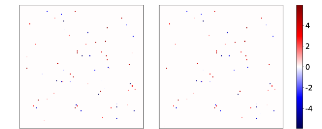
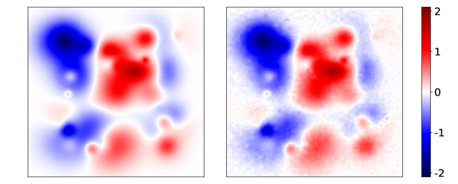
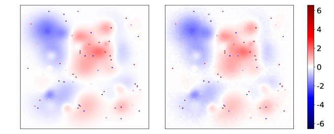
The source image is simulated as the sum of a sparse component, that is a set of bright isolated pixels, and a smooth component, simulated as a sum of low intensity gaussian functions with different spatial extensions (left panel of Figure 1). Both the sparse and smooth components take positive and negative values.
To handle this signal model, the penalty matrices are and as defined in (7). The forward matrix is chosen as the random DFT measurements of equation (6). In particular, the sampled frequencies are drawn at random, half of them following a gaussian distribution, the other half being uniformly distributed. This heterogeneous model allows to sample both the low and high frequencies of the signal, mimicking the sampling pattern of radio interferometry, which is consistent with the composite signal model. Indeed, the sparse component presents high frequency components and is thus difficult to reconstruct with low frequency samples only, and conversely for the smooth component . For an image of size pixels, the number of measurements is chosen as % of the number of measurements necessary to exactly reconstruct the image, that is . The simulated measurements are finally corrupted with an additive gaussian white noise with PSNR of dB.
Reconstructions are performed with Python, using the versatile optimization library Pyxu [19]. The coupled method directly solves the problem () of size with the APGD solver [14]. The decoupled approach also solves problem () of size with APGD, then the solution of the problem () is computed explicitly with its closed-form expression.


IV-B Parametrization of the regularization parameters
Setting the regularization parameters is of critical importance for the reconstruction of signal with optimization methods. From the decoupled problems in Theorem 1, we propose an interpretable and natural way to perform this critical choice. We introduce the dimensionless parameters and to parameterize respectively and , that need to be handpicked depending on the noise intensity and the signal model, but no longer on the dimensions of the problem.
For the parameter , it is known that there exists a maximum value above which any solution of a LASSO problem is [13]. It is then common to set the regularization parameter as
with . With the operators introduced in Section III, the sparse component problem () is a simple LASSO problem, so that we can compute the critical value
using the symmetry of the matrix .
As for the parameter , it can be interpreted with an analysis analogous to [10] (see (3.47), Section 3.4.1). Indeed, allows to modify the contribution of the reconstruction vectors depending on the associated singular value in the sampling matrix. For the smooth component problem (), the solution is expressed as
We then propose to set so that
where computes the maximum singular value of a matrix. The parameter controls the intensity of the regularization applied to the forward matrix , automatically scaling to the actual singular values of .
IV-C Analysis of the reconstructions
The solutions produced by the two methods are extremely similar, we provide the reconstruction from the decoupled approach in Figure 1. We notice that the sparse component is recovered with high accuracy, with a Jaccard index of . The smooth component also recovers the source with good accuracy, despite the grainy texture on the border of the shapes, displaying a relative error of with respect to the smooth component of the source.
With the decoupled approach, we usually notice a smaller value of the objective function and a sparser component. This behavior could be due to a finer convergence of the numerical solver. Indeed, the stopping criterion for APGD is set as a threshold on the relative improvement of the iterates. The presence of the two components in the iterates of size of the coupled approach may alter the actual value of this improvement compared to the decoupled approach, in which the optimization problem is run over only.
When less measurements are considered, the reconstruction of the smooth component is less accurate, however we observed that there is some robustness in the estimation of the sparse component. Similarly, when the image size increases, the grainy texture of becomes more visible, even when playing with the regularization parameter . For larger images, it could make sense to use a Laplacian kernel with larger support to promote greater smoothness.
IV-D Numerical performances
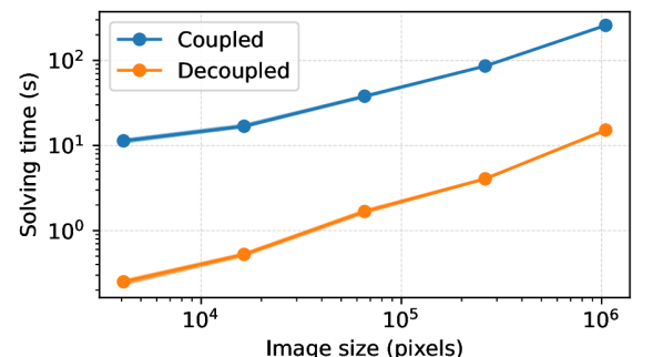
The most significant benefit of our RT lies in the speed efficiency of the decoupled approach. The solving times of the two methods are reported in Figure 2. The decoupled approach is significantly faster, achieving an acceleration factor of 17 for the largest images considered, and even better in smaller dimensions. This is explained by faster and less numerous iterations.
It should be noted that the specific setup considered here, involving a diagonal matrix , is particularly favorable for a fast decoupled approach. The efficiency gains might not be as striking in other contexts, but accelerations may still happen when and have simple expressions.

Acknowledgment
The authors would like to thank Lucas d’Alimonte and Martin Vetterli for help and support. This research was supported by the SNSF with the grant SESAM - Sensing and Sampling: Theory and Algorithms (n° 200021_181978/1.)
References
- [1] Alnur Ali and Ryan J. Tibshirani “The Generalized Lasso Problem and Uniqueness” In Electronic Journal of Statistics 13.2, 2019
- [2] Louis M. Briceño-Arias, Patrick L. Combettes, Jean-Christophe Pesquet and Nelly Pustelnik “Proximal Algorithms for Multicomponent Image Recovery Problems” In Journal of Mathematical Imaging and Vision 41.1, 2011, pp. 3–22
- [3] Ingrid Daubechies and Gerd Teschke “Variational Image Restoration by Means of Wavelets: Simultaneous Decomposition, Deblurring, and Denoising” In Applied and Computational Harmonic Analysis 19.1, 2005, pp. 1–16
- [4] Christine De Mol and Michel Defrise “Inverse Imaging with Mixed Penalties” In ULB Institutional Repository, 2004
- [5] Valentin Debarnot, Paul Escande, Thomas Mangeat and Pierre Weiss “Learning Low-Dimensional Models of Microscopes” In IEEE Transactions on Computational Imaging 7, 2021, pp. 178–190
- [6] Thomas Debarre, Shayan Aziznejad and Michael Unser “Continuous-Domain Formulation of Inverse Problems for Composite Sparse-Plus-Smooth Signals” In IEEE Open Journal of Signal Processing 2, 2021, pp. 545–558
- [7] Axel Flinth and Pierre Weiss “Exact Solutions of Infinite Dimensional Total-Variation Regularized Problems” In Information and Inference: A Journal of the IMA 8.3, 2019, pp. 407–443
- [8] Ali Gholami and S. Hosseini “A Balanced Combination of Tikhonov and Total Variation Regularizations for Reconstruction of Piecewise-Smooth Signals” In Signal Processing 93.7, 2013, pp. 1945–1960
- [9] Per Christian Hansen “Rank-deficient and discrete ill-posed problems: numerical aspects of linear inversion”, SIAM monographs on mathematical modeling and computation Philadelphia: SIAM, 1998
- [10] Trevor Hastie, Robert Tibshirani and Jerome H. Friedman “The Elements of Statistical Learning: Data Mining, Inference, and Prediction” Springer Science & Business Media, 2001
- [11] Martin Jaggi “Revisiting Frank-Wolfe: Projection-Free Sparse Convex Optimization” In Proceedings of the 30th International Conference on Machine Learning PMLR, 2013, pp. 427–435
- [12] Adrian Jarret, Julien Fageot and Matthieu Simeoni “A Fast and Scalable Polyatomic Frank-Wolfe Algorithm for the LASSO” In IEEE Signal Processing Letters 29, 2022, pp. 637–641
- [13] Alexandra Koulouri, Pia Heins and Martin Burger “Adaptive Superresolution in Deconvolution of Sparse Peaks” In IEEE Transactions on Signal Processing 69, 2021, pp. 165–178
- [14] Jingwei Liang, Jalal Fadili and Gabriel Peyré “Activity Identification and Local Linear Convergence of Forward–Backward-type Methods” In SIAM Journal on Optimization 27.1, 2017, pp. 408–437
- [15] Pina Marziliano, Martin Vetterli and Thierry Blu “Sampling and Exact Reconstruction of Bandlimited Signals with Additive Shot Noise” In IEEE Transactions on Information Theory 52.5, 2006, pp. 2230–2233
- [16] Valeriya Naumova and Steffen Peter “Minimization of Multi-Penalty Functionals by Alternating Iterative Thresholding and Optimal Parameter Choices” In Inverse Problems 30.12 IOP Publishing, 2014, pp. 125003
- [17] Stanley Osher, Andrés Solé and Luminita Vese “Image Decomposition and Restoration Using Total Variation Minimization and the H1” In Multiscale Modeling & Simulation 1.3 Society for Industrial and Applied Mathematics, 2003, pp. 349–370
- [18] Bixio Rimoldi “Principles of Digital Communication: A Top-Down Approach” Cambridge: Cambridge University Press, 2016
- [19] Matthieu Simeoni, Sepand Kashani, Joan Rué-Queralt and Pyxu Developers “pyxu-org/pyxu: pyxu” Zenodo URL: https://doi.org/10.5281/zenodo.4486431
- [20] Jean-Luc Starck, Michael Elad and David L. Donoho “Image Decomposition via the Combination of Sparse Representations and a Variational Approach” In IEEE Transactions on Image Processing 14.10, 2005, pp. 1570–1582
- [21] A. Thompson, James M. Moran and George W. Swenson “Interferometry and Synthesis in Radio Astronomy”, Astronomy and Astrophysics Library Cham: Springer International Publishing, 2017
- [22] Michael Unser and Shayan Aziznejad “Convex Optimization in Sums of Banach Spaces” In Applied and Computational Harmonic Analysis 56, 2022, pp. 1–25
- [23] Michael Unser, Julien Fageot and Harshit Gupta “Representer Theorems for Sparsity-Promoting Regularization” In IEEE Transactions on Information Theory 62.9, 2016, pp. 5167–5180
- [24] Martin Vetterli, Jelena Kovačević and Vivek K. Goyal “Foundations of Signal Processing” In Higher Education from Cambridge University Press Cambridge University Press, 2014