LHMap-loc: Cross-Modal Monocular Localization Using LiDAR Point Cloud Heat Map

Abstract

Localization using a monocular camera in the pre-built LiDAR point cloud map has drawn increasing attention in the field of autonomous driving and mobile robotics. However, there are still many challenges (e.g. difficulties of map storage, poor localization robustness in large scenes) in accurately and efficiently implementing cross-modal localization. To solve these problems, a novel pipeline termed LHMap-loc is proposed, which achieves accurate and efficient monocular localization in LiDAR maps. Firstly, feature encoding is carried out on the original LiDAR point cloud map by generating offline heat point clouds, by which the size of the original LiDAR map is compressed. Then, an end-to-end online pose regression network is designed based on optical flow estimation and spatial attention to achieve real-time monocular visual localization in a pre-built map. In addition, a series of experiments have been conducted to prove the effectiveness of the proposed method. Our code is available at: https://github.com/IRMVLab/LHMap-loc.

I Introduction

Localization is a critical technology [1] in autonomous driving and robotics that underlies other downstream tasks, such as navigation and control. Map-based localization is often utilized to alleviate the error caused by satellite signal blocking in GNSS localization methods[2, 3, 4] and the accumulated drift in Simultaneous Location And Mapping (SLAM) methods [5, 6, 7]. LiDAR is the primary sensor in constructing the map because point clouds are not affected by light changes in the environment. However, LiDAR sensors are expensive and tend to be large in size, while monocular cameras are small and inexpensive, making them easier to be equipped on mobile devices. Therefore, the technology of visual localization in LiDAR maps has broad application prospects.

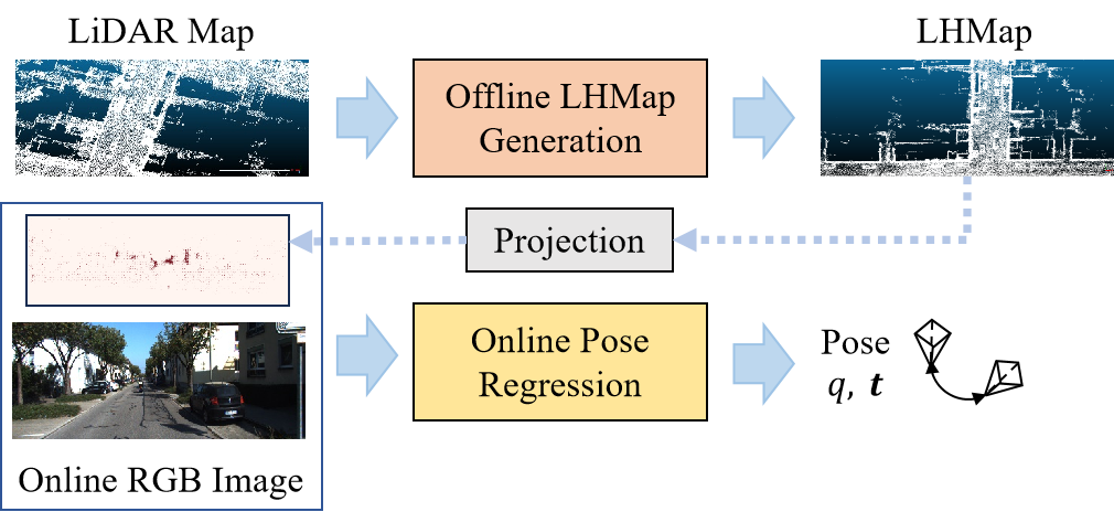
Figure 1: Monocular localization pipeline using LiDAR point cloud heat map (LHMap). The pipeline consists of an offline LHMap generation network to build LHMap, and an online pose regression network to achieve real-time localization with pre-built LHMap.

However, there are two main challenges regarding this technology. The first is the large consumption of storage and calculation for LiDAR maps. Since point clouds are disordered, it usually requires heavy computation to extract features from original LiDAR maps. The second challenge is the 3D-2D cross-modal feature matching. Since the point cloud maps contain 3D coordinate information, while the camera images contain 2D RGB pixels, feature matching cannot be carried out directly between the camera images and the point cloud maps. PnP based methods [8, 9] cannot provide reasonable solutions because the correspondence between 3D points and 2D pixel data is unknown. Besides, methods that generate 3D point clouds from 2D images for matching and regression [1, 10] suffer from depth inaccuracies. Recent HD map based localization methods [11, 12, 13] rely on specific geometric structures such as lane lines, road signs which may not appear in some rural roads or parks. Additionally, HD map annotations are time-consuming and labour-intensive. Therefore, HD map based methods are not suitable for all occasions.

To deal with the above problems, we propose a monocular localization pipeline termed LHMap-loc as shown in Fig. 1. We refer to the sorted and filtered LiDAR map as LiDAR point cloud Heat Map (LHMap). In this pipeline, LHMap generation is first conducted on the original LiDAR point cloud through offline supervised training, retaining the key features and compressing the point cloud map. Then, the 6 Degree-of-Freedom (DoF) poses are predicted by a pose regression network based on optical flow prediction and spatial attention weighting. In this end-to-end network, real-time high-precision pose regression is realized. The main contributions of this paper are as follows:

• We propose a monocular visual localization pipeline named LHMap-loc. This pipeline can compress and encode the features of the point cloud map in an offline way, and carry out monocular localization online. The whole pipeline is realized by the deep learning method.

• A pose regression algorithm based on optical flow prediction and spatial attention weighting is designed. The algorithm achieves a cross-modal fusion of 3D and 2D features, enabling end-to-end pose estimation.

• Numerous experiments have been conducted on the automatic driving datasets, KITTI [14] and Argoverse[15] datasets. In addition, we conduct real-world experiments on our own wheeled vehicle platform. The results show that the proposed LHMap-loc performs better in terms of precision and efficiency than the state-of-the-art (SOTA) methods[16, 17, 18, 19].

II Related Work

3D-2D cross-modal localization has always been a challenging task in terms of autonomous driving and robotics. The existing methods can be roughly divided into two categories according to the way of pose regression. One is the traditional methods which construct geometric residuals and calculate pose through mathematical optimization, and the other is the deep learning based methods which encode cross-model feature through MLPs and regress pose from neural networks.

II-A Geometric Optimization Based Localization

For the problem of monocular visual localization in pre-built maps, Caselitz et al. [1] utilizes the feature points generated by ORB-SLAM[20] to obtain 3D points. Then they utilize Iterative Closest Point (ICP) [21] methods to conduct point registration and compute the real-time poses. Yu et al. [22] first extract the line features in the monocular image and point cloud. They then achieve cross-modal localization by optimizing the distance and angle residuals between line segments. Ye et al.[23, 24] re-build the original point cloud as a Surfel map composed of Surfel descriptors, and then construct the visual-Surfel residual to proceed pose optimization. Similarly, Huang et al. [25] model map points using a Gaussian Mixture Model. Recently, Zhang et al. [10] propose to combine semantic point cloud for cross-modal localization. They first construct point cloud maps containing semantic information, and then perform registration and pose regression with the semantic ORB feature points constructed in real time. However, these methods have disadvantages. Firstly, visual features such as feature points and line segments are greatly affected by the lighting condition and are not robust enough, which is easy to cause mismatching. In addition, dynamic objects and irregular noisy points have a crucial impact on Surfel and GMM models during the construction of LiDAR maps.

II-B Deep Matching Based Localization

Due to the powerful feature coding capability of deep learning networks, Zhou et al. [26] encode the features of map points based on image heat maps, and then perform monocular localization through online pose regression. [16] propose the pose regression method based on 2D optical flow estimation for the first time. Then, Chang et al. [18] add LiDAR point cloud feature coding and voxel down-sampling modules on the basis of the original CMRNet[16]. CMRNet++ [17, 19] adds PnP module following CMRNet[16]. They estimate the point cloud and pixel matching relationship by 2D optical flow estimation, and then respectively adopt the EPnP [9] and BPnP[27] method to get the final pose. Miao et al. [28] propose a novel transformer-based neural network to register images to LiDAR maps, and introduce pose queries to boost the certainty of networks. However, these methods have some problems, such as excessive storage of point cloud maps, poor accuracy and low efficiency of pose regression.

III LHMap-loc Method

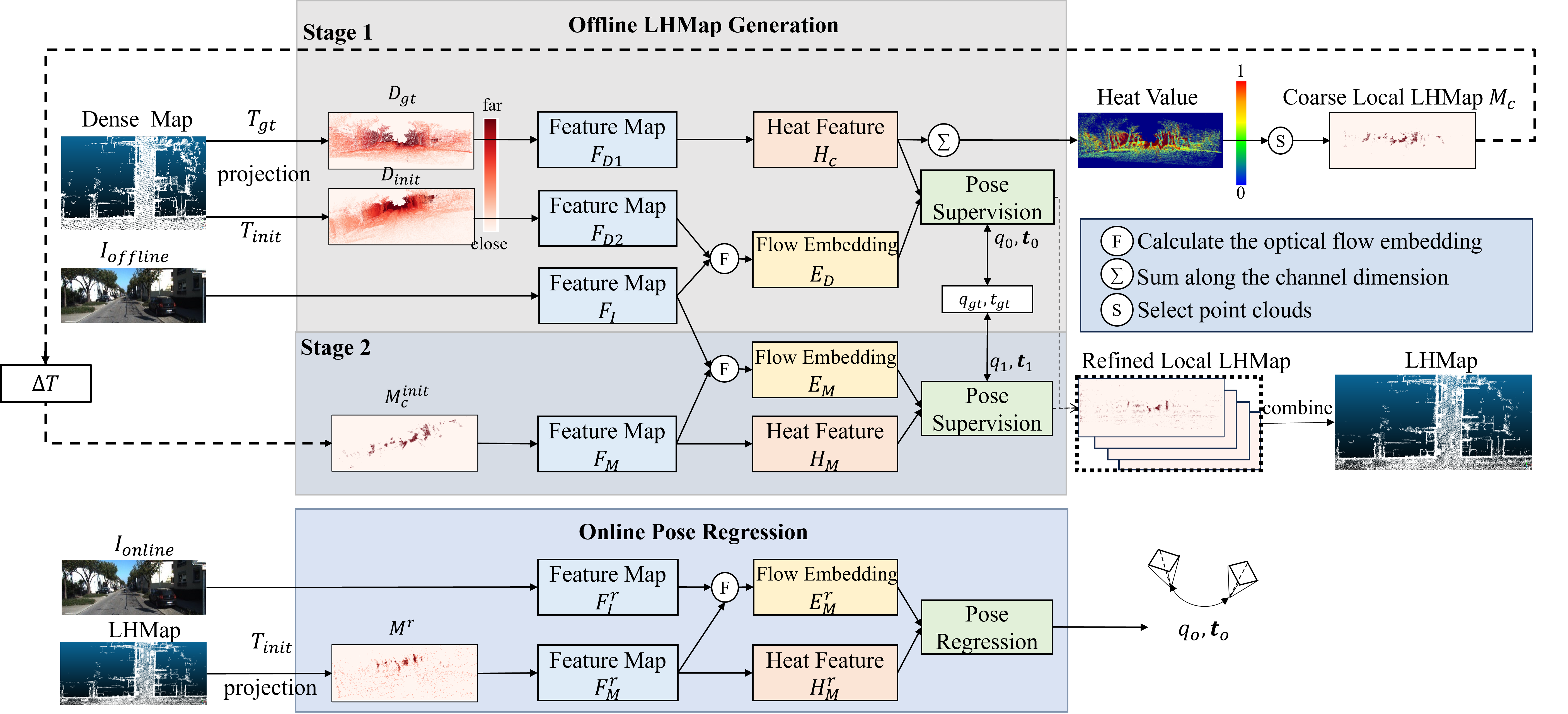
Figure 2: Detailed pipeline of LHMap-loc. It includes the offline LHMap generation network and the online pose regression network. In stage 1 of the offline network, $D_{gt}$ is used to generate heat feature $H_{c}$, and the coarse local LHMap $M_{c}$ is selected by the heat value calculated by $H_{c}$. $D_{init}$ and $I_{offline}$ are used to generate the flow embedding $E_{D}$. In stage 2, the initial coarse local LHMap $M_{c}^{init}$ and $I_{offline}$ are used to generate the flow embedding $E_{M}$ and the heat feature $H_{M}$. Both $E_{D}$ and $E_{M}$ are used for pose supervision by spatial attention weighting. In the online pose regression network, the real-time local LHMap $M_{r}$ and $I_{online}$ are used to regress the real-time 6-DoF pose.

III-A System Overview

As depicted in Fig. 2, the proposed LHMap-loc pipeline aims to locate the monocular camera image $I\in{\mathbb{R}^{3\times{h}\times{w}}}$ within the pre-built LiDAR point cloud map $P\in{\mathbb{R}^{3\times{n}}}$, where $h$ and $w$ represent the height and width of the image, respectively, and $n$ represents the number of 3D points in the map. In this pipeline, we realize cross-modal monocular localization through two main procedures: the offline LHMap construction procedure and the online pose regression procedure. Regarding the offline LHMap construction procedure, we feed the pre-built dense point cloud map $P$ and offline camera images into the network to construct the LHMap. During this procedure, the dense point cloud map is compressed while maintaining the key features used for localization. This procedure is described in detail in Sec. III-B. As for online pose regression, the LHMap and online RGB images are fed into an end-to-end network to regress the 6-DoF poses $q\in\mathbb{H},t\in\mathbb{R}^{3}$, where $q$ represents the quaternion and $t$ is the translation vector. We achieve real-time cross-modal localization based on 2D flow feature embedding and spatial attention weighting. This procedure is detailed in Sec. III-C.

III-B Offline LHMap Generation Network

As shown in Fig. 2, we use the offline LHMap generation network to compress the pre-built LiDAR point cloud map. It is realized through two stages.

In the first stage, we realize the point selection to compress the dense map and pose supervision to refine the generated local map. To satisfy the requirement for point selection and map compression, the projected LiDAR depth $D_{gt}$ is used to construct an evaluation system for point clouds. It is calculated as:

$$D_{gt}^{u,v}=z^{gt},$$ (1)

$$(u,v,1)^{T}=K\cdot(x^{gt},y^{gt},z^{gt},1)^{T}=K\cdot{T_{gt}^{-1}\cdot(x,y,z,1)^{T}}.$$ (2)

Here, $(x,y,z)\in P$, $K$ represents the camera intrinsics, and $T_{gt}\in SE(3)$ represents the ground truth camera pose at each frame. Additionally, the offline RGB image $I_{offline}$ and projected LiDAR depth $D_{init}$ are used to perform pose supervision. Based on the initial rough camera pose $T_{init}\in SE(3)$ at each frame, which can be acquired by GPS or visual odometry, $D_{init}$ is calculated as:

$$D_{init}^{u,v}=z^{init},$$ (3)

$$(u,v,1)^{T}=K\cdot(x^{init},y^{init},z^{init},1)^{T}=K\cdot{T_{init}^{-1}(x,y,z,1)^{T}}.$$ (4)

Here, $(x,y,z)^{T}\in P$. Both $D_{gt}$ and $D_{init}$ contain only the depth information of point clouds.

Firstly, feature maps $F_{I},F_{D1}$, and $F_{D2}$ with different scales are extracted from $I_{offline}$, $D_{gt}$, and $D_{init}$ respectively, through convolutional neural networks (CNN). $F_{D1}$, the CNN feature of the projected LiDAR depth $D_{gt}$ is used to generate the heat feature $H_{c}$. The point clouds are selected by evaluating heat value. Heat value is calculated by heat feature $H_{c}$ which is generated by $F_{D1}$. Each element $h_{k}^{i,j}\in H_{c}(i\in\{1,2,...,h\},j\in\{1,2,...,w\}$) is used to calculate heat value $h^{i,j}$ for point clouds evaluation as:

$$h^{i,j}=Mask^{i,j}\cdot\sum_{k=1}^{C}h_{k}^{i,j},$$ (5)

$$Mask^{i,j}=\left\{\begin{array}[]{ll}0,&M_{gt}^{i,j}=0\\ 1,&M_{gt}^{i,j}\neq 0\\ \end{array}.\right.$$ (6)

Here, $C$ represents the number of channels of $H_{c}$. Subsequently, points exhibiting the highest heat values are selected to constitute the coarse local LHMap, denoted as $M_{c}$.

$$M_{c}^{i,j}=TopN(h^{i,j}),$$ (7)

$$TopN(h^{i,j})=\left\{\begin{array}[]{ll}D_{gt}^{i,j},&if\ h^{i,j}\ ranking\ top\ N\\ 0,&others\\ \end{array}.\right.$$ (8)

During the generation of $M_{c}$, the pose supervision is adopted to guide the procedure. The pose supervision module incorporates two inputs: the heat feature $H_{c}$, and the optical flow embedding $E_{D}$, which is derived from $F_{D2}$ and $F_{I}$ based on the iterative optimization structure of PWCNet[29]. Pose supervision is realized by pose calculation module, detailed in Sec. III-C.

The single stage 1 learning fails to converge. Therefore, we propose the second stage to refine LHMap. In the second stage, we apply $\Delta T=T_{init}^{-1}\cdot T_{gt}$ to the coarse local LHMap $M_{c}$ to recover the initial localization results. The initial coarse local LHMap $M_{c}^{init}$ and the offline RGB image $I_{offline}$ are used for further pose supervision. Because both stages share the same offline RGB image, they share the same feature maps $F_{I}$ of the RGB image naturally, while the feature maps $F_{M}$ of the initial coarse local LHMap $M_{c}^{init}$ are regenerated. Then, the heat feature $H_{M}$ is generated by $F_{M}$ and the flow embedding $E_{M}$ is generated by $F_{M}$ and $F_{I}$. At last, they work together for pose supervision. Pose supervision is realized by the pose calculation module which is introduced in Sec. III-C. In this stage, we regress another set of 6-DoF pose $q_{1},t_{1}$. Both $q_{0},t_{0}$ and $q_{1},t_{1}$ refine the local LHMap by optimising the heat feature $H_{c}$.

The output of this network is the LiDAR point cloud Heat Map (LHMap) combined by the refined local LHMap at each frame. Though the local LHMap contains only the depth information, by taking the inverse of the projection formulation, we can obtain the 3D coordinates information $P_{k}$ at each frame $k$. With the knowledge of the ground truth camera pose ${}^{w}T_{k}$ at frame $k$ and the points $P_{k}$ of frame $k$, we can convert $P_{k}$ to the world frame:

$${}^{w}P_{k}={{}^{w}T_{k}}\cdot P_{k}.$$ (9)

Here, ${}^{w}P_{k}$ represents the points at the frame $k$ in the world coordinate system. The LHMap is constructed by uniting all the points ${}^{w}P_{k}$ together through an union operation $\cup_{k}$:

$$LHMap=\cup_{k}{{}^{w}P_{k}}.$$ (10)

The loss function of the offline heat map generation network is similar to CMRNet[16]. Let $q_{gt}$ and $t_{gt}$ represent the ground truth camera pose. The angular distance $L_{q}$ between quaternions is used to evaluate the rotation loss. The L1-smooth loss $L_{t}$ is used to evaluate the translation loss, which is defined as:

$$\mathcal{L}_{q}(q,\ q_{gt})=D(q\bigotimes{inv(q_{gt})}),$$ (11)

$$D(q)=\arctan((\sqrt{b^{2}+c^{2}+d^{2}},\ |a|)),$$ (12)

$$\mathcal{L}_{t}(t,\ t_{gt})=L_{1}smooth(t-t_{gt}),$$ (13)

Here, $\{a,b,c,d\}$ are the components of quaternion $q$ and $\bigotimes$ is the multiplicative operation between two quaternions. The pose loss is defined as:

$$\mathcal{L}_{p}=\mathcal{L}_{t}+\lambda\mathcal{L}_{q},\lambda\geq 1.$$ (14)

The pose $t_{0},q_{0}$ regressed by the pose supervision module in stage 1 and the pose $t_{1},q_{1}$ regressed by the pose supervision module in stage 2 are both taken into account for better supervision. Therefore, the total loss is defined as:

$$\mathcal{LOSS}_{1}=\alpha\mathcal{L}_{p0}+\beta\mathcal{L}_{p1},\ \alpha+\beta=1..$$ (15)

III-C Online Pose Regression Network

This network is used for real-time monocular localization. The inputs are the online RGB image $I_{online}$ and the real-time LHMap $M^{r}$. The $M^{r}$ is constructed by projecting ${}^{t}P$ at each local LHMap stored in the first network to the image plane according to the function in (4).

Firstly, feature maps $F_{I}^{r}$ and $F_{M}^{r}$ are extracted from both inputs $I_{online}$ and real-time local LHMap $M^{r}$ through convolutional neural networks (CNN).

Then, the feature maps $F_{M}^{r}$ are used to calculate the 2D flow embedding $E_{M}^{r}$ along with the RGB image feature maps $F_{I}^{r}$ and to generate the heat feature $H_{M}^{r}$ alone. $E_{M}^{r}$ here is calculated the same as PWCNet[29]. The usage of the heat feature $H_{M}^{r}$ enables the pose regression to focus on effective features. Therefore, the supervision of the 2D flow embedding $E_{M}^{r}$ and the regression of 6-DoF pose can achieve better performance. The cost volume $V$ is then calculated by feeding $H_{M}^{r}$ into the softmax layer to generate the coefficients and multiplying the coefficients with $E_{M}^{r}$. The cost volume $V$ is calculated as:

$$\mathcal{V}=\sum_{h\times w}{E_{M}^{r}\odot Softmax_{h\times w}(H_{M}^{r})},$$ (16)

where $\odot$ means element-wise product, $softmax_{h\times w}$ means apply softmax to height and width dimensions of $H_{M}^{r}$.

At last, the cost volume is fed into separate MLPs for pose regression:

$$q_{o}=MLP_{q}(V),\ \ t_{o}=MLP_{t}(V).$$ (17)

The pose regression is realized by the pose calculation module as shown in Fig. 3. The resolution of the flow feature may be different from that of the heat feature. Therefore, the flow feature is transferred to the up-sampled layers to maintain the same resolution as the heat feature before being multiplied with it. The multiplication result then accumulates all the elements across the height and width dimensions before being fed into fully connected layers, which are denoted as $MLP_{q}$ and $MLP_{t}$. The outputs of this network are 6-DoF poses $t_{o},q_{o}$.

The loss function used here follows [30]. Adding two trainable parameters $w_{x}$ and $w_{q}$, the loss function is defined as:

$$\mathcal{LOSS}_{2}=e^{-w_{x}}\mathcal{L}_{t}+w_{x}+e^{-w_{q}}\mathcal{L}_{q}+w_{q}.$$ (18)

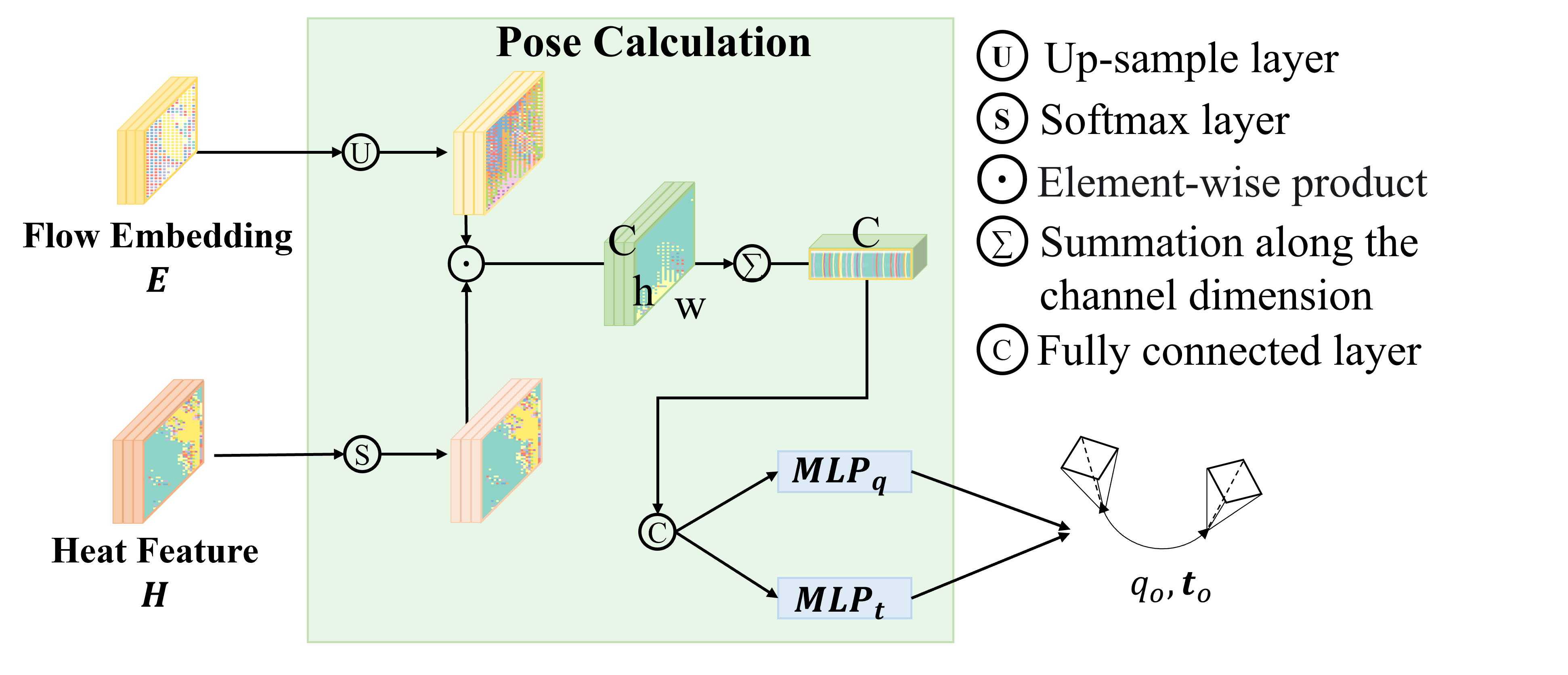
Figure 3: The details of the regression part. Multiply flow embedding $E$ and up-sampled heat feature $H$ as inputs, and then calculate weighted features. The result is fed into $MLP_{q}$ and $MLP_{t}$ to regress 6-DoF poses

III-D Training Details

We implement our network using PyTorch. For the offline heat map generation network, it is trained for 120 epochs using the ADAM optimizer, with a batch size of 8 and a learning rate of 1e-4. We apply the loss function as defined in (15), setting the parameters to $\lambda=10$, $\alpha=0.6$, and $\beta=0.4$. The top 5000 point clouds are selected for storage and further processing. For the online pose regression network, it is trained for 150 epochs, utilizing the Adam optimizer [31] with a batch size of 12 and a learning rate of 1e-4. The loss function (18) is employed with the initial values set to $w_{x}=0$ and $w_{q}=-2.5$. All training and evaluation activities are performed on a single NVIDIA GTX 2080 Ti.

IV Experiments

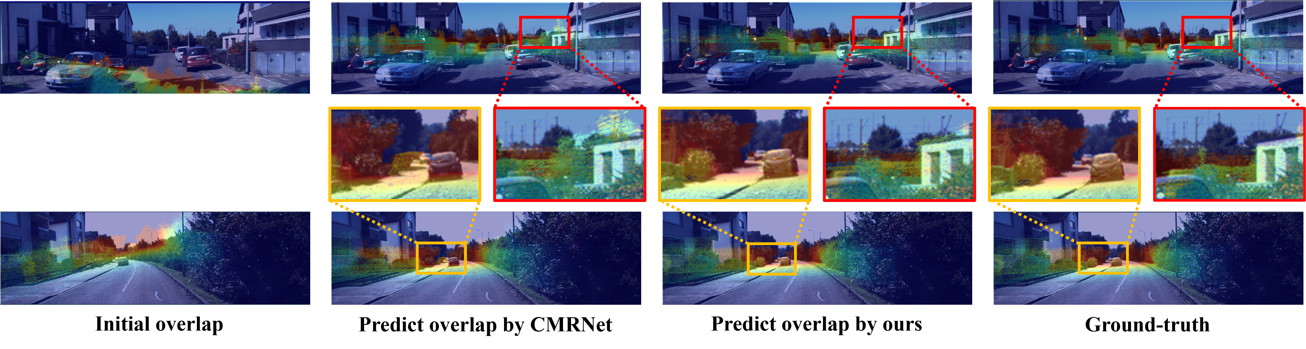
Figure 4: Qualitative results of LiDAR-image registration on KITTI[14] dataset.

TABLE I: Quantitative localization results of training and testing on single KITTI[14] and Argoverse[15] dataset

3		CMRNet[16]		HyperMap[18]		PosesAsQueires[28]		Ours
		Transl.[m]	Rot.[deg]	Transl.[m]	Rot.[deg]	Transl.[m]	Rot.[deg]	Transl.[m]	Rot.[deg]
KITTI[14]	Iter1	0.51	1.39	0.48	1.42	0.41	1.39	0.21	0.94
	Iter2	0.31	1.09	-	-	0.20	0.90	0.06	0.35
	Iter3	0.27	1.07	-	-	0.20	0.79	0.03	0.33
Argoverse[15]	Iter1	0.90	1.78	0.58	0.93	-	-	0.20	0.99
	Iter2	0.80	1.56	-	-	-	-	0.10	0.66
	Iter3	0.67	1.52	-	-	-	-	0.09	0.57
2.5

TABLE II: Quantitative results of methods using sharing weights on KITTI[14] and Argoverse[15] dataset

3		CMRNet++[17]			I2D-Loc[19]			Ours
		Transl.[m]	Rot.[deg]	failure rate[%]	Transl.[m]	Rot.[deg]	failure rate[%]	Transl.[m]	Rot.[deg]	failure rate[%]
	KITTI[14]	0.55	1.46	2.18	0.17	0.70	1.61	0.26	1.50	0
	Argoverse[15]	0.80	1.55	6.24	0.47	0.71	7.52	0.29	1.69	0
2.5

TABLE III: Ablation experiments on pose regression and Top N selection.

3	Method		Top N			Transl.[m]		Rot.[deg]
	CMRNet	ours	N = all	N = 10k	N = 5k	Mean	Median	Mean	Median
	✓		✓			0.57	0.51	1.80	1.39
	✓				✓	0.31	0.26	1.99	1.83
		✓	✓			0.64	-	1.92	-
		✓		✓		0.28	0.23	1.41	1.27
		✓			✓	0.25	0.21	1.04	0.94
2

TABLE IV: Performance comparison of different sources of heat feture.

3	Heat Map Generation			Transl.[m]		Rot.[deg]
	Randomly	RGB image	LiDAR depth	Mean	Median	Mean	Median
	✓			1.15	-	1.74	-
		✓		0.30	0.25	1.62	1.32
			✓	0.25	0.21	1.04	0.94
2

IV-A Datasets and Data Preprocessing

IV-A1 KITTI dataset [14]

The LiDAR maps, the ground truth poses, and the initial poses are generated following CMRNet[16] and HyperMap[18]. KITTI Odometry sequences 03, 05, 06, 07, 08 and 09 are selected to be the training set (11426 frames) and sequence 00 is the evaluation set (4541 frames). The methods for generating LiDAR maps and the projected LiDAR depth follow the same procedures as outlined in CMRNet[16].

IV-A2 Argoverse dataset [15]

Images from the central forward facing camera that provides $1920\times 1200$ images are used for localization on Argoverse dataset. These images are down-sampled to $960\times 600$ according to [17]. The ground-truth maps are built with voxel resolutions of 0.1m. Sequences train1, train2, train3, train4 and val are used as the training set (17614 frames), and the test sequence is used as the evaluation set (4168 frames). Besides, following [18], some frames affected dynamic objects are removed from the training set.

We also apply an iterative refinement approach following [16]. For the first iteration, we introduce uniformly distributed noise ranging from $[-2m,2m]$ for translation and $[-10^{\circ},10^{\circ}]$ for rotation to the ground truth poses $H_{gt}$. Subsequent noise levels are set to $[-1m,1m]$ with $[-2^{\circ},2^{\circ}]$ for the second iteration, and $[-0.6m,0.6m]$ with $[-1^{\circ},1^{\circ}]$ for the third iteration.

IV-B Performance

As for qualitative results, Fig. 4 exhibits the results of LiDAR-image registration using predicted poses between camera images and projected LiDAR depths. Compared with [16], our method can achieve better LiDAR-image registration with overlap patterns more similar to the ground-truth. Moreover, in regions with sparse features, our pipeline can also achieve robust pose regression thanks to the pre-built LHMap and the spatial attention weighting algorithm.

Table IV shows the quantitative monocular localization results of different methods under 3 iterations. For a fair comparison, all methods listed in the table follow the same selection of the training set and the test set. With regard to the KITTI dataset and Argoverse dataset, our pipeline enables more accurate monocular localization evaluated by both translation and rotation errors by a large margin compared with the SOTA methods: CMRNet[16], HyperMap[18], and PosesAsQueires[28]. Moreover, one iteration of our method yields even higher localization accuracy than three iterations of CMRNet. In addition, our method achieves a more significant accuracy improvement during iterative optimization.

Besides, Fig. 5 displays the visualisation results of the point cloud map on KITTI sequence 00 with the voxel size equals to 0.1m. As shown in Fig. 5, the generated LHMap retains the main structural features of the point cloud. Compared with the original map, our LHMap compresses the map by 80%. Meanwhile, LHMap achieves better performance for monocular localization due to its effective feature extraction.

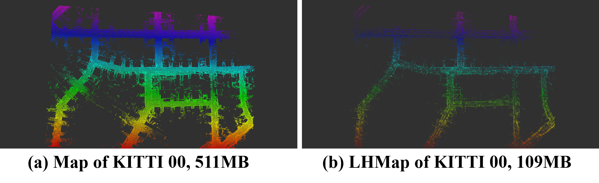
Figure 5: 3D point cloud map of KITTI sequence 00. (a) Original LiDAR point cloud map. (b) LHMap.

We also conduct experiments on projecting the RGB image and the projected LiDAR depth to the normalization plane, which aims to achieve mapping and monocular localization with different cameras. In this procedure, we first convert every pixel in the RGB image and every point in the point cloud map to the normalization frame. Then we map $\{(x,y)|-0.8<x<0.8,-0.4<y<0.4\}$ in the normalization coordinate to the image plane $\{(u,v)|0\leq u<768,0\leq v<384\}$. Then, we train the pipeline on KITTI sequences 03, 05, 06, 07, 08, 09 and Argoverse sequences Train1, Train2, Train3, and test on KITTI sequence 00 and Argoverse sequence Train4 following [19]. The results are shown in Table II. According to CMRNet++[17], we define the situation as a failure if the translation error is larger than 4m. The results demonstrate that our methods achieve competitive localization accuracy especially on Argoverse. Remarkably, our failure rate is zero on both KITTI and Argoverse. It is demonstrated that our method is more robust to challenging environments such as rural roads lacking structured geometry features.

IV-C Ablation Study

To verify the contribution of key modules in our LHMap-loc pipeline, a series of ablation experiments are designed. The experiments are mainly carried out from three aspects: the strategy of heat map generation, the density of LHMap and the method of pose regression. We thoroughly evaluate all methods on the KITTI dataset[14] with one iteration. And the results are as shown in Table III and Table IV.

First of all, in Table III different pose regression modules are tested in the online pose regression network using different $TopN$ mapping points per frame. We select $N=all$, $N=10000$ and $N=5000$ points separately and $N=5000$ achieves even better localization results than the other two cases. The pose regression module is also replaced by CMRNet, and the results demonstrate that our improvements are effective.

Additionally, we test on different ways to generate LHMap. In Table IV, heat features generated by the RGB image are leveraged instead of the projected LiDAR depth to construct LHMap. Offline maps are also generated by random selection. The experiments demonstrate that our LHMap generation strategy achieves better localization accuracy.

TABLE V: comparison of Time consumption in each method

3   Time/ms	CMRNet	CMRNet++	I2D-loc	PosesAsQueries	Ours
Pre-process Time	101.890	-	-	-	1.844
Inference Time	6.868	1250.	80.	-	11.079
Total	109.910	$>$1250.	$>$80.	14.925	13.402
2

IV-D Time Consumption

Localization has a strict requirement for real-time performance, therefore we test the time consumption in the process of pose regression. The pre-process time, which includes the time for data loading, projecting and occlusion filtering and inference time are evaluated and displayed in Table IV-C. Every sample is tested and averaged on KITTI sequence 00 with batch size equals to 1. The results demonstrate our network can perform pose regression at about 77 frames per second (FPS), while CMRNet spends much more time in pre-processing data. In conclusion, our methods spend much less time in localization than [16], [17], [19] and [28].

IV-E Real-world Experiments

To validate our methods in real-world scenarios, we collect data using a Hesai PandarXT-16 LiDAR and an industrial camera (MV-CA013-21UC) at Shanghai Jiao Tong University (SJTU), specifically around the lake and the administration building. The data is further processed by FAST-LIO[5] and RTK to acquire ground truth poses and the pre-built point cloud map. It is noteworthy that the collected scenarios are challenging. Because these scenarios are primarily composed of trees and shrubbery, while lacking the buildings like KITTI and Argoverse. Meanwhile, the equipment is carried on a low-speed, remote-controlled vehicle, as shown in Fig. 6, which means the field of view of the LiDAR and camera is entirely different from that of KITTI and Argoverse. In the SJTU dataset, our methods also achieve extremely accurate localization results, as shown in Table VI, not affected by changing scenarios. Overall, our methods demonstrate robustness in facing the challenges of real-world scenarios.

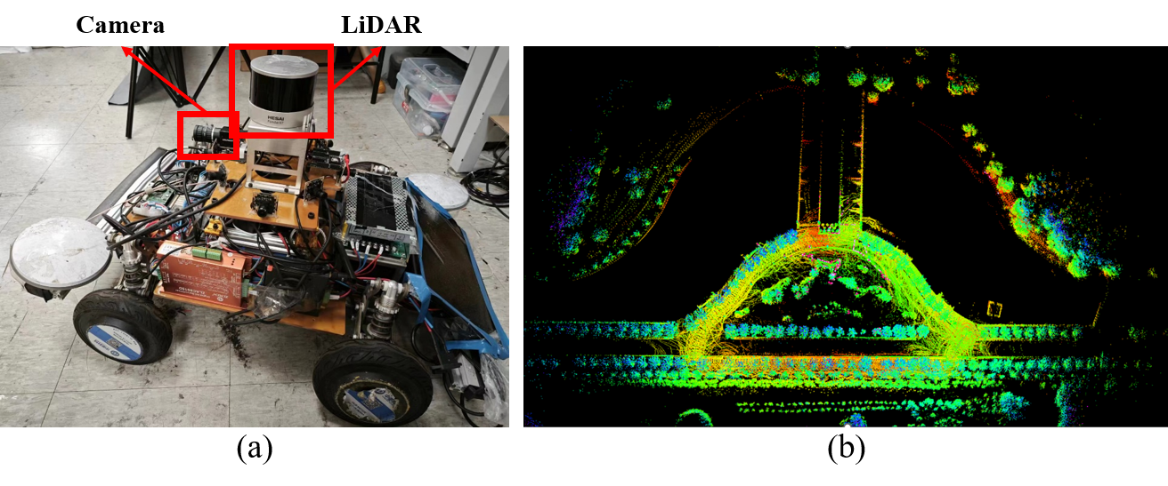
Figure 6: (a) The wheeled vehicle for SJTU-dataset collection.   (b) One scenario of SJTU-dataset.

TABLE VI: Localization results in SJTU-dataset

3	Transl.[m]		Rot.[deg]		Map size
	Mean	Median	Mean	Median
CMRNet(All Points)	0.95	0.86	1.66	1.42	197.99MB
Ours (All Points)	1.02	0.95	0.72	0.64	197.99MB
Ours (5k Points)	0.22	0.19	1.01	0.85	39.51MB
2

V Conclusion

This paper uses offline heat map generation network to construct LHMap. Further, online pose regression is realized by an end-to-end pose regression network for LHMap and real-time RGB images. Through extensive experimental results, the effectiveness of LHMap is demonstrated in improving localization accuracy and reducing the size of LiDAR maps. Overall, to our knowledge, the proposed LHMap-loc in this paper achieves higher accuracy and is more robust than SOTA learning-based monocular localization.

References

- [1] T. Caselitz, B. Steder, M. Ruhnke, and W. Burgard, “Monocular camera localization in 3d lidar maps,” in 2016 IEEE/RSJ International Conference on Intelligent Robots and Systems (IROS). IEEE, 2016, pp. 1926–1931.
- [2] D. Wang, C. Gao, S. Pan, and Y. Yang, “A robust strategy for ambiguity resolution using un-differenced and un-combined gnss models in network rtk,” The Journal of Navigation, vol. 69, no. 3, pp. 504–520, 2016.
- [3] J. Zumberge, M. Heflin, D. Jefferson, M. Watkins, and F. Webb, “Precise point positioning for the efficient and robust analysis of gps data from large networks,” Journal of geophysical research: solid earth, vol. 102, no. B3, pp. 5005–5017, 1997.
- [4] X. Zou, M. Ge, W. Tang, C. Shi, and J. Liu, “Urtk: undifferenced network rtk positioning,” GPS solutions, vol. 17, pp. 283–293, 2013.
- [5] W. Xu, Y. Cai, D. He, J. Lin, and F. Zhang, “Fast-lio2: Fast direct lidar-inertial odometry,” IEEE Transactions on Robotics, vol. 38, no. 4, pp. 2053–2073, 2022.
- [6] J. Lin and F. Zhang, “R 3 live: A robust, real-time, rgb-colored, lidar-inertial-visual tightly-coupled state estimation and mapping package,” in 2022 International Conference on Robotics and Automation (ICRA). IEEE, 2022, pp. 10 672–10 678.
- [7] C. Zheng, Q. Zhu, W. Xu, X. Liu, Q. Guo, and F. Zhang, “Fast-livo: Fast and tightly-coupled sparse-direct lidar-inertial-visual odometry,” in 2022 IEEE/RSJ International Conference on Intelligent Robots and Systems (IROS). IEEE, 2022, pp. 4003–4009.
- [8] R. Haralick, D. Lee, K. Ottenburg, and M. Nolle, “Analysis and solutions of the three point perspective pose estimation problem,” in Proceedings. 1991 IEEE Computer Society Conference on Computer Vision and Pattern Recognition, 1991, pp. 592–598.
- [9] V. Lepetit, F. Moreno-Noguer, and P. Fua, “Ep n p: An accurate o (n) solution to the p n p problem,” International journal of computer vision, vol. 81, pp. 155–166, 2009.
- [10] C. Zhang, H. Zhao, C. Wang, X. Tang, and M. Yang, “Cross-modal monocular localization in prior lidar maps utilizing semantic consistency,” in 2023 IEEE International Conference on Robotics and Automation (ICRA), 2023, pp. 4004–4010.
- [11] H. Wang, C. Xue, Y. Zhou, F. Wen, and H. Zhang, “Visual semantic localization based on hd map for autonomous vehicles in urban scenarios,” in 2021 IEEE International Conference on Robotics and Automation (ICRA). IEEE, 2021, pp. 11 255–11 261.
- [12] H. Wang, C. Xue, Y. Tang, W. Li, F. Wen, and H. Zhang, “Ltsr: Long-term semantic relocalization based on hd map for autonomous vehicles,” in 2022 International Conference on Robotics and Automation (ICRA). IEEE, 2022, pp. 2171–2178.
- [13] K. Petek, K. Sirohi, D. Büscher, and W. Burgard, “Robust monocular localization in sparse hd maps leveraging multi-task uncertainty estimation,” in 2022 International Conference on Robotics and Automation (ICRA). IEEE, 2022, pp. 4163–4169.
- [14] A. Geiger, P. Lenz, C. Stiller, and R. Urtasun, “Vision meets robotics: The kitti dataset,” The International Journal of Robotics Research, vol. 32, no. 11, pp. 1231–1237, 2013.
- [15] M.-F. Chang, J. Lambert, P. Sangkloy, J. Singh, S. Bak, A. Hartnett, D. Wang, P. Carr, S. Lucey, D. Ramanan, et al., “Argoverse: 3d tracking and forecasting with rich maps,” in Proceedings of the IEEE/CVF conference on computer vision and pattern recognition, 2019, pp. 8748–8757.
- [16] D. Cattaneo, M. Vaghi, A. L. Ballardini, S. Fontana, D. G. Sorrenti, and W. Burgard, “Cmrnet: Camera to lidar-map registration,” in 2019 IEEE intelligent transportation systems conference (ITSC). IEEE, 2019, pp. 1283–1289.
- [17] D. Cattaneo, D. G. Sorrenti, and A. Valada, “Cmrnet++: Map and camera agnostic monocular visual localization in lidar maps,” arXiv preprint arXiv:2004.13795, 2020.
- [18] M.-F. Chang, J. Mangelson, M. Kaess, and S. Lucey, “Hypermap: Compressed 3d map for monocular camera registration,” in 2021 IEEE International Conference on Robotics and Automation (ICRA). IEEE, 2021, pp. 11 739–11 745.
- [19] K. Chen, H. Yu, W. Yang, L. Yu, S. Scherer, and G.-S. Xia, “I2d-loc: Camera localization via image to lidar depth flow,” ISPRS Journal of Photogrammetry and Remote Sensing, vol. 194, pp. 209–221, 2022.
- [20] R. Mur-Artal, J. M. M. Montiel, and J. D. Tardos, “Orb-slam: a versatile and accurate monocular slam system,” IEEE transactions on robotics, vol. 31, no. 5, pp. 1147–1163, 2015.
- [21] P. Besl and N. D. McKay, “A method for registration of 3-d shapes,” IEEE Transactions on Pattern Analysis and Machine Intelligence, vol. 14, no. 2, pp. 239–256, 1992.
- [22] H. Yu, W. Zhen, W. Yang, J. Zhang, and S. Scherer, “Monocular camera localization in prior lidar maps with 2d-3d line correspondences,” in 2020 IEEE/RSJ International Conference on Intelligent Robots and Systems (IROS). IEEE, 2020, pp. 4588–4594.
- [23] H. Ye, H. Huang, and M. Liu, “Monocular direct sparse localization in a prior 3d surfel map,” in 2020 IEEE International Conference on Robotics and Automation (ICRA). IEEE, 2020, pp. 8892–8898.
- [24] H. Ye, H. Huang, M. Hutter, T. Sandy, and M. Liu, “3d surfel map-aided visual relocalization with learned descriptors,” in 2021 IEEE International Conference on Robotics and Automation (ICRA). IEEE, 2021, pp. 5574–5581.
- [25] H. Huang, H. Ye, Y. Sun, and M. Liu, “Gmmloc: Structure consistent visual localization with gaussian mixture models,” IEEE Robotics and Automation Letters, vol. 5, no. 4, pp. 5043–5050, 2020.
- [26] Y. Zhou, G. Wan, S. Hou, L. Yu, G. Wang, X. Rui, and S. Song, “Da4ad: End-to-end deep attention-based visual localization for autonomous driving,” in Computer Vision–ECCV 2020: 16th European Conference, Glasgow, UK, August 23–28, 2020, Proceedings, Part XXVIII 16. Springer, 2020, pp. 271–289.
- [27] B. Chen, A. Parra, J. Cao, N. Li, and T.-J. Chin, “End-to-end learnable geometric vision by backpropagating pnp optimization,” in Proceedings of the IEEE/CVF Conference on Computer Vision and Pattern Recognition, 2020, pp. 8100–8109.
- [28] J. Miao, K. Jiang, Y. Wang, T. Wen, Z. Xiao, Z. Fu, M. Yang, M. Liu, and D. Yang, “Poses as queries: Image-to-lidar map localization with transformers,” 2023.
- [29] D. Sun, X. Yang, M.-Y. Liu, and J. Kautz, “Pwc-net: Cnns for optical flow using pyramid, warping, and cost volume,” in Proceedings of the IEEE conference on computer vision and pattern recognition, 2018, pp. 8934–8943.
- [30] Q. Li, S. Chen, C. Wang, X. Li, C. Wen, M. Cheng, and J. Li, “Lo-net: Deep real-time lidar odometry,” in Proceedings of the IEEE/CVF Conference on Computer Vision and Pattern Recognition, 2019, pp. 8473–8482.
- [31] D. P. Kingma and J. Ba, “Adam: A method for stochastic optimization,” arXiv preprint arXiv:1412.6980, 2014.