Constraints on Metastable Dark Energy Decaying into Dark Matter

Abstract

We revisit the proposal that an energy transfer from dark energy into dark matter can be described in field theory by a first order phase transition. We analyze the model proposed in Ref. Abdalla:2012ug , using updated constraints on the decay time of a metastable dark energy from the work of Ref. Shafieloo:2016bpk . The results of our analysis show no prospects for potentially observable signals that could distinguish this scenario. We also show that such model would not drive a complete transition to a dark matter dominated phase even in a distant future. Nevertheless, the model is not excluded by the latest data and we confirm that the mass of the dark matter particle that would result from such a process corresponds to an axion-like particle, which is currently one of the best motivated dark matter candidates. We argue that extensions to this model, possibly with additional couplings, still deserve further attention as it could provide an interesting and viable description for an interacting dark sector scenario based in a single scalar field.

I Introduction

One of the main goals of physical cosmology has been to understand the nature of the constituents of our Universe, especially the dark matter (DM) and dark energy (DE) which, together, constitute nearly 96$\%$ of the total density of the Universe. Many theoretical models have been developed to explain the nature of the dark Universe Sahni:2004ai . The DM component, due to its clustering properties, has been investigated in the context of several astrophysical and cosmological experiments. Moreover, unlike the case of DE, it has also been studied at particle physics level, being sought in direct detectors on Earth. In this context, one of the most interesting possibilities is that the DM can be an axion-like particle (a good review on axion-like dark matter can be found in Ref. Ferreira:2020fam , for instance), which is one of the main candidates for this component today. On the other hand, the nature of the DE component remains yet very obscure, despite there have been important advances in modeling its behavior beyond the simple cosmological constant scenario.

The explanation for a late-time accelerated phase in the Universe remains topic of much debate, which is related to the well known cosmological constant problem d28dd6a75fda4c2eb0aa9e85b7da702e ; Martin:2012bt . In a different framework, there are many challenges when trying to embed such models in a more fundamental quantum gravity proposal. As an example we can mention the Swampland conjecture, which describes a whole inhabitable landscape of field theories that are inconsistent with string theory, including the stable de-Sitter vacua Palti:2019pca ; Heisenberg:2018rdu ; Heisenberg:2018yae . In the process of trying to understand the DE properties, we are faced with the recurring discussion in the literature concerning the issue of the stability of a de-Sitter phase. In the context of the late time Universe, a stable de-Sitter phase has shown either to be hard to achieve from fundamental physics or even to be inconsistent in different theoretical contexts. For example, it has been subject of a long debate whether a de-Sitter space is unstable due to infrared (IR) effects, as conjectured in Refs. Polyakov:2007mm ; Polyakov:2012uc ; Valiviita:2008iv ; Mazur:1986et ; Mottola:1985ee , for instance. An instability of a de-Sitter phase has also been obtained as a consequence of backreaction effects of super-Hubble modes. As shown in several works Brandenberger:2018fdd ; Abramo:1997hu ; Mukhanov:1996ak ; Finelli:2001bn ; Finelli:2003bp ; Marozzi:2006ky ; Brandenberger:1999su , the backreaction of super-Hubble modes could give a negative contribution to the effective cosmological constant, causing the latter to relax.

From the observational point of view, one motivation for investigating possibilities beyond the cosmological constant solution is the current tension in $H_{0}$ measurements, which has shown to be alleviated in some quintessence models, as well as in models with dark sector interaction deSa:2022hsh ; DiValentino:2019exe ; DiValentino:2019ffd ; Zhao:2017cud . Concerning the latter, in the framework of field theory it can be argued to be rather natural to consider an interaction between DM and DE, given that they are fundamental fields of the theory. Interacting models can also been claimed as a proposal for alleviating the coincidence problem Weinberg:2000yb , while also being able to provide good fit to current data Ferreira:2014jhn ; Amendola:1999er ; Valiviita:2008iv ; Abdalla:2009mt ; Faraoni:2014vra ; He:2008tn ; Costa:2013sva ; Benetti:2021div .

In a related framework, when going beyond the cosmological constant scenario, its natural to investigate the possibility of a metastable DE. As pointed out in Ref. Shafieloo:2016bpk , the remarkable qualitative similarity between the properties of the present DE and the component that supposedly drove inflation in the very early Universe makes it rather natural to put forward the hypothesis that the current DE can also be metastable Shafieloo:2016bpk ; Urbanowski:2021waa ; Urbanowski:2022iug ; Landim:2016isc ; Landim:2017lyq ; Stojkovic:2007dw ; Greenwood:2008qp ; Abdalla:2012ug . In this context, in Ref. Shafieloo:2016bpk metastable DE phenomenological models were analyzed, in which the DE decay rate does not depend on external parameters, being assumed to be a constant depending only on DE intrinsic properties. They considered data from BAO SDSS:2009ocz ; Anderson:2012sa ; Beutler:2011hx ; BOSS:2014hwf and Supernovae Type Ia SupernovaCosmologyProject:2011ycw , and found that the typical decay time in these scenarios must be many times larger than the age of the Universe. One possible theoretical model that can provide a field theory description for the class of phenomenological scenarios considered in the analysis of Ref. Shafieloo:2016bpk is the model proposed in Ref. Abdalla:2012ug , hereafter referred as MDE (Metastable Dark Energy) model. In this MDE model, a positive “cosmological constant” is modeled by a non zero scalar vacuum energy with a potential of the expected order $V\approx 10^{-47}{\rm GeV}$ in the false vacuum. The potential of the scalar field in this model has a doubly degenerated energy minima with small symmetry breaking term that provide such a small energy difference . In this scenario the field at the false vacuum represents DE. After the field passes the potential barrier, decaying from the false to the true vacuum, its equation of state is no longer that of a dark energy, as it acquires a non negligible kinetic energy . Analogously to what happens in the old inflationary scenario, the transition to the true vacuum occurs through the formation of bubbles of new vacuum Callan:1977pt ; Coleman:1977py . Through this process, the energy released in the conversion of the false vacuum into the true can produce a new component, which has the properties of DM. In the previous work of Ref. Abdalla:2012ug , it was shown that the mass of the DM in this scenario would correspond to an axion-like particle, however, for a decay time of DE on the order of the age of the Universe, as assumed in the work of Ref. Abdalla:2012ug . Being the axion one of the main candidates for DM today Ferreira:2020fam ; Amin:2022nlh ; Nadler:2021dft ; Irsic:2017yje ; Dalal:2022rmp ; Powell:2023jns ; Semertzidis:2021rxs ; Nakai:2022dni ; Nakatsuka:2022gaf ; QUAX:2020uxy ; Cicoli:2021gss ; Harigaya:2019qnl , it motivates us to further explore this model in the light of the new constraints Shafieloo:2016bpk .

Here we revisit the MDE model using the new constraints from Ref. Shafieloo:2016bpk , in order to test if the model is still viable and whether the newly constrained decay time still predicts the same mass for the DM particle produced in this scenario. As discussed above, due to the similarities of the current DE and the primordial inflation, one of our main goals is also to check if this model inherits the same problems of old inflation GUTH1983321 ; PhysRevD.46.2384 , i.e, potentially observable inhomogeneities from the process of bubble nucleation and evolution.

In particular, we aim to address the following questions:

1) Is MDE still a viable model considering the latest cosmological constraints?

2) What is the mass of the DM resulting from this process?

3) Would the bubble nucleation process in this model lead to inhomogeneities that could plague the model?

4) Could this model leave observational imprints that could be searched for in future experiments?

In order to address these questions we organize the paper as follows: In Sec. II we present the MDE model proposed in Ref. Abdalla:2012ug to describe an interacting dark sector model based on field theory. In Sec. III we compute the mass of the DM particle of this model that results from the DE decay with a characteristic time compatible with the recent constraints from Ref. Shafieloo:2016bpk . In Sec. IV we analyze the bubble nucleation process and its subsequent dynamics in order to see if the model would predict observable inhomogeneities. In Sec. V we conclude and discuss some future prospects. In Appendix A we demonstrate the validity of the approximations considered.

II A Model for Dark Energy Decay

In this section we present the MDE model proposed in Abdalla:2012ug to describe an interacting dark energy model based on field theory. Since the model contemplates an energy exchange between dark energy and dark matter, none of these components is separately conserved. The equations describing the model are written as,

$$\dot{\rho}_{\rm DE}+3H\rho_{\rm DE}(1+\omega_{\rm DE}) = Q_{\rm DE},$$ (1)

$$\dot{\rho}_{\rm DM}+3H\rho_{\rm DM}(1+\omega_{\rm DM}) = Q_{\rm DM},$$ (2)

where dot denotes the derivative with respect to cosmic time, $\omega_{i}$ is the equation of state parameter (EoS), $H$ is the Hubble parameter, $Q_{i}$ is the interaction term and the subscript $i$ indicates DE or DM.

We consider that $Q_{i}$ is linearly proportional to the energy density of DE Abdalla:2012ug :

$$Q_{\rm DM}=-Q_{\rm DE}=\Gamma\,\rho_{\rm DE}$$ (3)

In the model we are going to consider, the DE decay rate, $\Gamma$, does not depend on external parameters such as the curvature of the Universe or the scale factor. Instead, the DE decay rate is assumed to be a constant (similar to the case of the radioactive decay of unstable particles and nuclei).

Once the interaction term is defined, we can write an effective EoS for DE,

$$\omega_{\rm DE}^{\rm(eff)}=\omega_{\rm DE}+\frac{\Gamma}{3H}.$$ (4)

From Eq. (4), we see that in a DE-DM interaction model the effective EoS can have a phantom-like behavior ($\omega^{\rm(eff)}_{\rm DE}<-1$) when the decay rate is negative (energy flow DM $\to$ DE), or a quintessence-like behavior ($\omega^{\rm(eff)}_{\rm DE}>-1$) when the decay rate is positive (energy flow DE $\to$ DM), which is our focus.

In the MDE model, DE is represented by a scalar field with a potential energy endowed with doubly degenerated minima. When a small symmetry breaking term is added, a small energy difference between the degenerate minima emerges. The DE responsible for the current expansion of the Universe is represented by the scalar field at the metastable minima, where the potential energy is adjusted to $V_{0+}\sim 10^{-47}\textrm{GeV}^{4}$. Such potential can be written as,

$$V(\phi)=\left|2m\phi-3\lambda\phi^{2}\right|^{2}+Q(\phi),$$ (5)

where $\phi=\varphi+iB$ is a complex scalar field of mass $m$ and coupling constant $\lambda$ and $Q(\phi)$ is the symmetry-breaking term, which is adjusted so that we have the value of cosmological constant at the metastable minimum . The first term corresponds to the bosonic sector of the Wess-Zumino Lagrangian and the potential is adjusted such that the stable minimum is the zero of the potential. Considering the bosonic field uncharged ($B=0$), the potential has minima at $\varphi=0$ and $\varphi=\frac{2m}{3\lambda}$. The general shape of the potential is shown in Fig. 1. Following the previous work Abdalla:2012ug we will consider the value $\lambda=10^{-2}$ for the coupling constant.

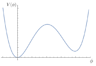
Figure 1: Shape of the potential $V(\phi)$.

In the case we are interested, with $\Gamma>0$ and energy flowing from the cosmological constant into dark matter, it follows that the value of the dark matter density parameter extrapolated to high redshifts would be higher than the value predicted by $\Lambda$CDM, while the expansion rate would be lower than that in $\Lambda$CDM. If the energy transfer occurs in a non-negligible rate this affects cosmological observables, the reason why it is important to consider observational constraints on such scenario.

In the work of Ref. Shafieloo:2016bpk a generic model of metastable DE decaying into DM was analyzed and constraints on the value of the decay rate were obtained. They considered three combinations of datasets in their analysis: (i) Firstly they used the Union-2.1 compilation  SupernovaCosmologyProject:2011ycw jointly with BAO data from SDSS DR7 (z = 0.35) SDSS:2009ocz , BOSS DR9 (z = 0.57) Anderson:2012sa and 6DF (z = 0.106) Beutler:2011hx . (ii) Next, they added to (i) BAO measurements of H(z) data at z = 2.34, namely H(2.34) BOSS:2014hwf . (iii) In the last analysis they included to (ii) the values for the CMB shift parameters from Ref. Planck:2013pxb . These three analyses constrained, respectively, the values: (i) $\Gamma/H_{0}=0^{+0.039}_{-0.028}$ (mean with 1$\sigma$ deviation); (ii) $\Gamma/H_{0}=0.04^{+0.34}_{-0.3}$ ; (iii) $\Gamma/H_{0}=-0.015\pm 0.02$. More details on their analysis and methodology can be found in Shafieloo:2016bpk . Recalling that the decay rate is the inverse of the decay time, this shows that the current constraints imply in a lifetime of the metastable DE greater than the age of the universe.

We are going to consider the aforementioned constraints in order to compute, in the next section, the mass of the dark matter particle that will result from such a process in the MDE model. It will become clear that the results are not so sensitive to the specific limit on $\Gamma$ chosen among the results presented above.

III Dark matter from first order phase transition

The energy transfer in the MDE model occurs due to the tunneling from the metastable (false) to the stable (true) vacuum of the potential, Eq. (5). This process can be described by a first order phase transition according to the semi-classical method developed in Refs. Coleman:1977py ; Callan:1977pt . Using this framework we are going to compute the mass of the resulting DM particle as a function of $\Gamma$.

The decay rate (per unit volume) reads,

$$\frac{\Gamma}{V}=\frac{S_{E}^{2}({\tilde{\varphi}}(\rho))}{(2\pi\hslash)^{2}}\times e^{-\left(\frac{S_{E}}{\hslash}-\frac{S_{\Lambda}}{\hslash}\right)}\times\left[\frac{det^{\prime}(-\partial_{\mu}\partial_{\mu}+V^{\prime\prime}({\tilde{\varphi}}(\rho))}{det(-\partial_{\mu}\partial_{\mu}+V^{\prime\prime}(\varphi_{+}))}\right]^{-\frac{1}{2}},$$ (6)

where $\varphi_{+}$ is the field amplitude at the false vacuum and ${\tilde{\varphi}}(\rho)$ is, in analogy with the case of particles, the classical field amplitude in Euclidean space crossing the potential $-V(\varphi)$ subject to boundary conditions $\varphi_{\rm initial}=\varphi_{\rm final}=\varphi_{+}$. $S_{E}$ is the Euclidean action and $S_{\Lambda}$ is the Euclidean action of a particle at the false vacuum. Looking for an analytical solution we will consider the so-called thin wall approximation Coleman:1977py ; Callan:1977pt as done in the previous work of Ref. Abdalla:2012ug . In this approximation the energy difference between the two minima of the potential, given by the parameter $\epsilon$, is considered to be small, then perturbative results can be obtained in terms of $\epsilon$.

The classical equation of motion in the Euclidean space for the field $\varphi$ subject to the potential $V(\varphi)$ is obtained by the minimization of $S_{E}$, which reads,

$$\frac{\delta S_{E}(\varphi(x))}{\delta\varphi}=-\partial_{\mu}\partial_{\mu}\varphi(x)+V^{\prime}(\varphi)=0.$$ (7)

We also suppose that

$$\displaystyle\lim_{\tau\rightarrow{\pm}\infty}\varphi(\vec{x},\tau)=\varphi_{+},$$ (8)

where $\tau=-it$.

The solution is Euclidean invariant, which means that $\varphi(\vec{x},\tau)=\varphi(({|\vec{x}|^{2}}+\tau^{2})^{\frac{1}{2}})$. Defining $\rho\equiv(|\vec{x}|^{2}+\tau^{2})^{\frac{1}{2}}$, the equation of motion now reads,

$$\frac{\partial^{2}\varphi}{\partial\rho^{2}}+\frac{3}{\rho}\frac{\partial}{\partial\rho}\varphi-V^{\prime}(\varphi)=0,$$ (9)

which is analogous to the equation of motion of a particle at position $\varphi$ as a function of time $\rho$, subject to a potential $-V(\varphi)$ and a friction term.

The decay process occurs by the formation of bubbles of true vacuum surrounded by the false vacuum outside. The field is at rest both inside and outside, and the friction-like term, $\frac{3}{\rho}\frac{\partial}{\partial\rho}\varphi$, is nonzero only at the bubble wall. Therefore, in the case the wall is thin we can consider that $\rho=R$ at the wall, being $R$ the bubble radius (see Refs. Coleman:1977py ; Callan:1977pt for further details). Finally, for a small energy difference $\epsilon$, the quantity $R=\rho$ is large and the friction coefficient $1/\rho\to 0$, then we can neglect the friction term also at the bubble wall. From these considerations, Eq. (9) now reads,

$$\frac{\partial^{2}\varphi}{\partial\rho^{2}}=V^{\prime}(\varphi).$$ (10)

Then, considering the potential in Eq. (5), the value of the field is each region is,

$$0 ,\quad 0<\rho\ll R,$$ (11a)

$$\tilde{\varphi} ,\quad\rho\approx R,$$ (11b)

$$2m/3\lambda ,\quad\rho\gg R,$$ (11c)

which corresponds to the regions inside the bubble ($0<\rho\ll R$), at the thin wall ($\rho\approx R$) and outside the bubble ($\rho\gg R$).

Now we compute the action by adding the separated contribution of each region, which reads,

$$S\equiv S_{E}-S_{\Lambda} \approx 2\pi^{2}\intop_{0}^{R-\Delta}d\rho\,\rho^{3}(-\epsilon)+2\pi^{2}\intop_{R-\Delta}^{R+\Delta}d\rho\,\rho^{3}\left[\frac{1}{2}\left(\frac{d\tilde{\varphi}}{d\rho}\right)^{2}+U\right]+2\pi^{2}\intop_{R+\Delta}^{\infty}d\rho\,\rho^{3}(0)\,$$ (12)

$$= -2\pi^{2}\epsilon\frac{R^{4}}{4}+2\pi^{2}R^{3}\intop_{R-\Delta}^{R+\Delta}d\rho(\frac{1}{2}(\frac{d\tilde{\varphi}}{d\rho})^{2}+U)+0$$

$$= -\frac{\pi^{2}R^{4}}{2}\epsilon+2\pi^{2}R^{3}S_{1},$$

where $\Delta$ represents the width of the wall, and we defined,

$$S_{1}\equiv\intop_{R-\Delta}^{R+\Delta}d\rho\left[\frac{1}{2}\left(\frac{d\tilde{\varphi}}{d\rho}\right)^{2}+U\right].$$ (13)

Minimizing the action $S$ with respect to $R$, one obtains:

$$\frac{dS}{dR}=-2\pi^{2}R^{3}\epsilon+6\pi^{2}R^{2}S_{1}=0,$$ (14)

which gives the solution,

$$R=\frac{3S_{1}}{\epsilon}.$$ (15)

For small $\epsilon$, integrating Eq. (10) we obtain $\frac{\partial}{\partial\rho}\varphi=\sqrt{2U}$. Using this expression and considering the Wess-Zumino potential, Eq. (5), from Eq. (16) one obtains:

$$S_{1}=\sqrt{2}\left(\frac{4m^{3}}{27\lambda^{2}}\right).$$ (16)

Finally, using Eq. (16) in Eq. (12), the action will result in:

$$S\approx\frac{m^{12}}{\lambda^{8}\epsilon^{3}}.$$ (17)

In the decay rate expression, Eq. (6), the exponential term will dominate. We also know the pre-exponential term has the dimension of energy to the $4th$ power and that it will weigh the overall value, then we simply estimate it as $1\,{\rm GeV}^{4}$ in order to provide correct units. Therefore, Eq. (6) can be written as:

$$\frac{\Gamma}{V}=m^{4}e^{-m^{12}/(\lambda^{8}\epsilon^{3})}.$$ (18)

Finally, by substituting the values of $\epsilon$ and $\lambda$, we obtain for the decay rate (per volume),

$$\frac{\Gamma}{V}=e^{-10^{156}(\frac{m}{{\rm GeV}})^{12}}{\rm GeV}^{4}.$$ (19)

Due to the symmetry of our problem, we can invert $\Gamma/V$, take its fourth root and interpret it as the decay time, $t_{\rm decay}$. If we equate the decay time to the age of universe, $t_{\rm 0}=10^{17}{\rm s}$, as was done in Ref. Abdalla:2012ug , the value $m\sim 10^{-13}\,{\rm GeV}$ is obtained. This result implies in a resulting axion-like DM particle Abdalla:2012ug . Knowing that the axion is one of the main candidates for DM today, we felt motivated to further explore this model in the light of the new cosmological data Shafieloo:2016bpk .

In order to do so, let us now consider the case when the inverse decay rate is not equated to the age of the Universe, but to an arbitrary decay time. We parameterize this case by introducing the parameter $\alpha$ assuming arbitrary values smaller than 1. If we consider the inverse of $\Gamma/V$ to be related to the age of the universe $t_{0}$, the quantity $\alpha\,(\Gamma/V)$ will imply in a decay time of the form $t_{\rm 0}/(\alpha)^{1/4}$. As a consequence, different choices of the parameter $\alpha$ (different choices of the decay rate/decay time) result in different values for the mass $m$ of the DM particle.

In Figure 2, we illustrate the dependence of the mass of the resulting DM particle on $\alpha$, with $\alpha$ ranging from $10^{-10}$ to $10^{-1}$. From this figure, we notice that there is no change in the order of magnitude of the mass for this whole range of values of $\alpha$.

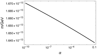
Figure 2: Dependence of the mass on the parameter $\alpha$, with the latter ranging from $10^{-10}$ to $10^{-1}$.

The behavior shown in Figure 2 can be described by the analytical expression,

$$m(\alpha)=1.12246\times 10^{-13}\sqrt[12]{94.8245-\ln\,\alpha},$$ (20)

which shows the weak dependence of the mass on $\alpha$. The order of magnitude of the mass only changes for $\alpha\sim 10^{-107598}$, which corresponds to a decay time $10^{26900}t_{\rm 0}$. Obviously, such a case is not interesting for us. Therefore, for any non-negligible (and observationally allowed) decay rate, the prediction for the DM mass, $m\sim 10^{-13}\,{\rm GeV}$, remains consistent.

As it’s well known, first-order phase transitions occur through random nucleation of bubbles. In this process, firstly the false vacuum energy is transferred to the kinetic energy of the bubbles wall, which asymptotically expands at the speed of light Coleman:1977py ; TeppaPannia:2016hwv ; Simon:2009nb ; Fischler:2007sz . However, in some cases, at some point, the walls of these bubbles may percolate, and the energy of the walls is converted into particles (energy density) that eventually thermalize hawking1982bubble ; PhysRevD.46.2384 ; kosowsky1992gravitational ; PhysRevD.84.024006 . Let us analyze this process further in the following section.

IV Bubble Nucleation

First order phase transitions, as the one considered here, occur through the nucleation and growth of bubbles of new phase.  This is similar to the process that happens in old inflationary models. In the case of old inflation, in order for the decay process to occur efficiently it was necessary an inflaton decay rate higher than a certain minimum value, in order to end inflation successfully. However, such a high decay rate would imply in a bubble nucleation process which leads to a highly inhomogeneous Universe. Given the similarities between the phase transition described here and the process that plagued the old inflationary model, we think it is important to discuss some implications of such process in the context of the model considered here.

In our low-temperature late time model for the dark sector, the bubble nucleation occurs through Coleman-Callan tunneling and the nucleation rate is essentially temperature-independent. Therefore, we consider the idealized model for the transition described in Ref. GUTH1983321 , in which the Universe is taken to be always at zero temperature, with negligible curvature. We can also approximately consider a de-Sitter exponential expansion, $a(t)\propto e^{H\,t}$, in the late time Universe, being $H$ the Hubble parameter assumed to be approximately constant. This is a sufficiently good approximation for our practical purposes. The de Sitter approximation can also be justified by the fact that the recent constraints that we are considering for the decay time implies in a decay process that will only be effective in a distant future, when the Universe is even more close to a de Sitter expansion.

We consider that bubble nucleation begins at a time $t_{B}$, and afterward occurs at a constant rate per unit of physical volume $\Gamma/V_{0}$. The decay rate per unit of coordinate volume is then given by $\Gamma(t)/V=(\Gamma/V_{0})\textrm{e}^{3Ht}$. We can consider the approximation in which bubble starts expanding from a very small radius $r_{0}\ll\,H^{-1}$. In order to show that this is the case, let us estimate the initial radius of the bubble from which it starts expanding. Using Eqs. (15) and (16), we can estimate this radius to be,

$$R_{0}=\sqrt{2}\left(\frac{12m^{3}}{27\lambda^{2}\epsilon}\right)\approx 10^{-2}\textrm{cm},$$ (21)

where in the last equality we used the particle mass determined in Sec. III, $m\approx 10^{-13}{\rm GeV}$, together with the values $\lambda=10^{-2}$ and $\epsilon=10^{-47}{\rm GeV}^{4}$.

In a successful first-order phase transition most of the bubbles are nucleated and collide in a time interval comparable to or shorter than the Hubble time. Those are the so-called fast transition, in which the nucleation rate is comparable to the expansion rate of the Universe GUTH1983321 ; PhysRevD.46.2384 . After bubbles collide, in the successful cases, the distribution of energy in the Universe becomes homogeneous as the relevant bubbles are sub-horizon sized when they collide. In the slow transitions, those in which the nucleation rate is much smaller then the expansion rate of the Universe, which we will show to be the case of the MDE model considered here, rare and very large bubbles are nucleated in a cosmological time. These bubbles can grow to astrophysical sizes and their dynamics covers a much longer period of time. After such bubble is nucleated, it soon starts expanding at the speed of light Coleman:1977py ; Callan:1977pt . For a bubble that emerges at a point $(t_{B},\vec{x}_{0})$ with a very small radius, at a later time $t$ its radius will be given by,

$$r(t,t_{B})=\left|\vec{x}-\vec{x}_{0}\right|=\int_{t_{B}}^{t}dt^{\prime}a(t^{\prime})^{-1}\;.$$ (22)

Evaluating the integral above gives us the result $r(t,t_{B})=H^{-1}(\textrm{e}^{-Ht_{B}}-\textrm{e}^{-Ht})$. We can see that the bubble radius will asymptotically assume the finite value,

$$r_{A}\equiv\lim_{t\rightarrow\infty}r(t,t_{B})=H^{-1}\textrm{e}^{-Ht_{B}},$$ (23)

hence, the volume of the Universe occupied by this bubble will asymptotically be,

$$V_{\textrm{asym}}=\frac{4\pi}{3H^{3}}\textrm{e}^{-3Ht_{B}}\;.$$ (24)

Due to the approximately de-Sitter expansion, the bubble will grow in comoving size for only about a $H^{-1}$ time, and after that, being super-Hubble, it simply stretches with the scale factor as the universe expands. This suggests that independently from the time past after the nucleation, two bubbles that emerge simultaneously at points $(t_{B},\vec{x}_{0}^{\prime})$ and $(t_{B},\vec{x}_{0}^{\prime\prime})$ at a proper distance $D=a(t_{B})\times\left|\vec{x}_{0}^{\prime}-\vec{x}_{0}^{\prime\prime}\right|>2H^{-1}$ will never percolate.

It is possible to analyze the evolution of the bubble distribution in the Universe by investigating the physical volume remaining in the false vacuum, given by $V_{phys}\propto a^{3}(t)p(t)$, where $p(t)$ is the probability that a given point in space is in the false vacuum at a time $t$. The quantity $p(t)$ can be written in the following form Guth:1979bh ; Guth:1981uk ; Guth:1980zm ; PhysRevD.46.2384 ; GUTH1983321 ,

$$p(t)=\textrm{e}^{-I(t)}\;,$$ (25)

where $I(t)$ is the expected volume of true-vacuum bubbles per unit volume of space at time $t$ . For a phase transition beginning at time $t_{0}$, we can expect this volume to be given, at time $t$, by the expression,

$$I(t)=\frac{4\pi}{3}\int^{t}_{t_{0}}dt^{\prime}(\Gamma/V_{0})a^{3}(t^{\prime})r^{3}(t,t^{\prime})\;.$$ (26)

where it was considered a constant decay rate $\Gamma$ for the MDE model. Above, $r(t,t^{\prime})$ is the coordinate radius at time t of a bubble that was nucleated at a time $t^{\prime}$, expressed in Eq. (22). Note that we are integrating in the nucleation times. Above we considered that the decay rate in the MDE model is a constant.

The equation above can be better understood if we view the quantity $I(t)$ as a function of the scale factor rather than $t$. In this case we can rewrite the equation above as,

$$I(t)=\frac{4\pi}{3}\int^{R(t)}_{R_{0}}da\frac{(\Gamma/V_{0})}{H}a^{2}\left(\int^{R(t)}_{a}da^{\prime}\frac{1}{a^{\prime 2}H}\right)^{3}\;.$$ (27)

Above we used Eq. (22) for $r(t,t^{\prime})$. The integrals in this expression are dominated by the upper limit of the integration range. We can see that the quantity $(\Gamma/V_{0})/H^{4}$ sets the magnitude of $I(t)$. Up to a numerical factor, this quantity measures the fraction of space occupied by large bubbles, which is given by $1-p(t)$. Therefore, provided that this fraction is small, as it will be in all cases of interest, $1-p(t)\approx I(t)$.

Even expanding at the speed of light, a bubble which nucleates at a time $t_{B}$ can only grow to a finite comoving radius radius given by Eq. (23) . Then, as shown above, if the separation between two bubbles at time $t$ is greater than 2$r_{A}$, the bubbles will never meet. Therefore the bubbles nucleated in a time interval of duration of $H^{-1}$ can never fill space by themselves, but instead only occupy a fraction of order $(\Gamma/V_{0})/H^{4}$ of the region which remained in the old phase at the time that they were nucleated. Although bubble nucleation continues indefinitely, and despite the physical volume of the old phase region (proportional to $a(t)^{3}p(t)$) is an increasing function of time, the bubbles produced have smaller and smaller comoving volume and so can fit in the remaining regions of old phase without overlapping.

Another simple way of understanding this is remembering that after a bubble is nucleated and grown to a size of about a Hubble radius, its size simply conformally stretches as the Universe expands. Then from that point on, the volume fraction of the Universe that it occupies remains constant. The volume fraction occupied by the bubbles nucleated during the time interval $\Delta t=H^{-1}$ is roughly the volume of a bubble when it begins conformally stretching, which is around $H^{-3}$, times the number of such bubbles nucleated in this interval per unit volume given by $\Gamma/(V_{0}H)$. Therefore the quantity $(\Gamma/V_{0})/H^{4}$ indicates the volume fraction of space occupied by bubbles nucleated over a Hubble time at a given epoch. We will denote by $\xi$ this important quantity,

$$\xi\equiv\frac{\Gamma/V_{0}}{H^{4}}.$$ (28)

A slow transition is considered to be the one in which the quantity above is much smaller than one, $\xi\ll 1$, and the Coleman-Callan tunneling is the only significant mechanism of bubble nucleation. When this is not the case, the transition is considered to be fast.

As discussed previously, the current data constraints the decay time to be around $t_{\rm decay}\gtrsim t_{0}/0.085$ (considering the higher best fit value among the results obtained in the analysis performed in Shafieloo:2016bpk ). We can then consider the approximate limit $t_{\rm decay}\gtrsim 10\,t_{0}$.

The decay time in our model is given by the quantity $t_{\rm decay}=(\Gamma/V)^{-1/4}$. Therefore we can write the quantity $\xi$ today to be given by

$$\xi=\frac{t_{\rm decay}^{-4}}{t_{0}^{-4}}\lesssim\left(\frac{t_{0}}{10\,t_{0}}\right)^{4}\;\;\;\;\;\;\;\rightarrow\;\;\;\;\;\;\;\;\xi\lesssim 10^{-4},$$ (29)

where in the second equality we considered the limit $t_{\rm decay}\gtrsim 10\,t_{0}$. We can see from the above equation that $\xi\ll 1$, proving that we are in the regime of slow transition.

We can hence conclude that such model will not drive a complete transition to a dark matter dominated phase. Even in the future, there will be a dominant region of the universe in the metastable phase, where we would still have an approximately de Sitter expansion. However, unlike old inflation, there is no observational restriction imposing that a complete transition from the dark energy state into dark matter must take place.

V Conclusion and Prospects

We considered the model proposed in Ref. Abdalla:2012ug , in which an energy transfer from dark energy into dark matter is described in field theory by a first order phase transition. We further investigate this model in light of the recent cosmological data. We find that the model is not excluded by the data, although it is non-falsifiable. Since the recent data constraints a decay time for the metastable dark energy that is considerably larger than the age of the Universe, it leaves no prospects for currently observing the result of the decaying DE process, which we showed to be an axion-like dark matter with mass $m\sim 10^{-13}{\rm GeV}$.

In particular, in this work, we provided the following answers to some, until now, open questions:

1) Considering the recent cosmological data, the model proposed in Ref. Abdalla:2012ug can still be considered, formally, a viable model for describing an unified dark sector.

2) The recent constraints in the decay time of the metastable dark energy imply in a resulting DM with a mass of an axion-like particle, although this resulting DM would only appear in the far future.

3) We do not expect this model to lead to observational imprints that could be searched for in future experiments, unless extra couplings are added to the Lagrangian of the model.

4) The bubble nucleation process was analyzed and we showed that the model considered, besides not leading to current observable inhomogeneities, would not drive a complete transition to a dark matter dominated phase, even in the far future.

Despite this model does not currently inherit the characteristics of a typical interacting dark sector model due to the large decay time, it still presents some qualitative advantages, as it is able to describe a dark sector in a unified manner through a single scalar field. In addition, the fact that around the true vacuum, this field behaves as a DM consistent with one of the best motivated DM candidates, gives us an indication of the potential of the model. For these reasons, we believe that possible extensions of this model deserve further investigation, as they could lead to potentially observables signatures in case additional couplings are included to the model Lagrangian (in this context see for example the works of Refs. Landim:2016isc ; Landim:2017lyq ). Furthermore, there is evidence from different theoretical contexts that exact de-Sitter solutions with a positive cosmological constant may not be suitable to describe the late-time universe. DE models based on scalar fields evolving in time are more promising in this regard, although in the context of the Swampland conjecture for example, they still have to satisfy certain criteria Palti:2019pca ; Heisenberg:2018rdu ; Heisenberg:2018yae . Verifying whether extensions of the model here consider could satisfy these and other theoretical conjectures, and leave observable traces, is an issue left for a future work.

Appendix A Gravitational Effects

In this Appendix we will discuss whether it is necessary to include corrections in the action due to gravitational effects. In order to investigate these effects, let us work with the following action,

$$\bar{S}=\int d^{4}x\sqrt{-g}\left(\frac{1}{2}g^{\mu\nu}\partial_{\mu}\varphi\partial_{\nu}\varphi-V(\varphi)-\frac{\mathcal{R}}{16\pi G}\right)\;,$$ (30)

where $\mathcal{R}$ is the curvature scalar. Using the thin wall approximation, which is still valid for the action (30) in the cases of interest, its straightforward to show the following relation between the action $\bar{S}$ and the action $S_{0}$ without gravitational effects Coleman:1980aw ,

$$\bar{S}=\frac{S_{0}}{\left[1+\left(\frac{R_{0}}{2\Delta}\right)^{2}\right]^{2}}\;.$$ (31)

Above $R_{0}$ is the initial radius of the bubble calculated in Eq. (21) and $\Delta$ is the Schwarzschild radius associated to the bubble of new vacuum, which is given by $\Delta=2G\epsilon(4\pi R_{0}^{3}/3)$. The expression for $\Delta$ can be understood from the fact that in the decay process from the metastable vacuum with energy $\epsilon$ to the stable vacuum with zero energy, there exists liberation of energy proportional to the energy density of the metastable vacuum and the volume of the nucleated new vacuum bubble. From Eq. (31) we can see that if $R_{0}/\Delta\sim 1$ we need to consider gravitational effects in our calculations. The gravitational effects will be important when the radius of the new vacuum bubble is of the order of the Schwarzschild radius. We can obtain the radius of a nucleated bubble that would be is equal to its Schwarzschild radius by equating $R_{0}=\Delta$, which gives us

$$R_{0}=\sqrt{\frac{3}{8\pi G\epsilon}}\;.$$ (32)

Using Eqs. (12) and (16) we can see that such initial radius would correspond to the decay of a particle with a mass of order $m\sim 10^{-2,8}\,\textrm{GeV}$, which is much heavier than the particle we obtained. Therefore the addition of gravitational effects would not significantly alter the results we obtained.

- [1] Elcio Abdalla, L. L. Graef, and Bin Wang. A Model for Dark Energy decay. Phys. Lett. B, 726:786–790, 2013.
- [2] Arman Shafieloo, Dhiraj Kumar Hazra, Varun Sahni, and Alexei A. Starobinsky. Metastable Dark Energy with Radioactive-like Decay. Mon. Not. Roy. Astron. Soc., 473(2):2760–2770, 2018.
- [3] Varun Sahni. Dark matter and dark energy. Lect. Notes Phys., 653:141–180, 2004.
- [4] Elisa G. M. Ferreira. Ultra-light dark matter. Astron. Astrophys. Rev., 29(1):7, 2021.
- [5] Mustafa A. Amin and Mehrdad Mirbabayi. A lower bound on dark matter mass. 11 2022.
- [6] Ethan O. Nadler, Simon Birrer, Daniel Gilman, Risa H. Wechsler, Xiaolong Du, Andrew Benson, Anna M. Nierenberg, and Tommaso Treu. Dark Matter Constraints from a Unified Analysis of Strong Gravitational Lenses and Milky Way Satellite Galaxies. Astrophys. J., 917(1):7, 2021.
- [7] Vid Iršič, Matteo Viel, Martin G. Haehnelt, James S. Bolton, and George D. Becker. First constraints on fuzzy dark matter from Lyman- forest data and hydrodynamical simulations. Phys. Rev. Lett., 119(3):031302, 2017.
- [8] Neal Dalal and Andrey Kravtsov. Excluding fuzzy dark matter with sizes and stellar kinematics of ultrafaint dwarf galaxies. Phys. Rev. D, 106(6):063517, 2022.
- [9] Devon M. Powell, Simona Vegetti, J. P. McKean, Simon D. M. White, Elisa G. M. Ferreira, Simon May, and Cristiana Spingola. A lensed radio jet at milli-arcsecond resolution II: Constraints on fuzzy dark matter from an extended gravitational arc. 2 2023.
- [10] Yannis K. Semertzidis and SungWoo Youn. Axion dark matter: How to see it? Sci. Adv., 8(8):abm9928, 2022.
- [11] Yuichiro Nakai, Ryo Namba, and Ippei Obata. Peaky Production of Light Dark Photon Dark Matter. 12 2022.
- [12] Hiromasa Nakatsuka, Soichiro Morisaki, Tomohiro Fujita, Jun’ya Kume, Yuta Michimura, Koji Nagano, and Ippei Obata. Stochastic effects on observation of ultralight bosonic dark matter. 5 2022.
- [13] D. Alesini et al. Realization of a high quality factor resonator with hollow dielectric cylinders for axion searches. Nucl. Instrum. Meth. A, 985:164641, 2021.
- [14] Sean M. Carroll, William H. Press, and Edwin L. Turner. The cosmological constant. Annual Review of Astronomy and Astrophysics, 30(1):499–542, 1992.
- [15] Jerome Martin. Everything You Always Wanted To Know About The Cosmological Constant Problem (But Were Afraid To Ask). Comptes Rendus Physique, 13:566–665, 2012.
- [16] Eran Palti. The Swampland: Introduction and Review. Fortsch. Phys., 67(6):1900037, 2019.
- [17] Lavinia Heisenberg, Matthias Bartelmann, Robert Brandenberger, and Alexandre Refregier. Dark Energy in the Swampland II. Sci. China Phys. Mech. Astron., 62(9):990421, 2019.
- [18] Lavinia Heisenberg, Matthias Bartelmann, Robert Brandenberger, and Alexandre Refregier. Dark Energy in the Swampland. Phys. Rev. D, 98(12):123502, 2018.
- [19] A. M. Polyakov. De Sitter space and eternity. Nucl. Phys. B, 797:199–217, 2008.
- [20] A. M. Polyakov. Infrared instability of the de Sitter space. 9 2012.
- [21] Jussi Valiviita, Elisabetta Majerotto, and Roy Maartens. Instability in interacting dark energy and dark matter fluids. JCAP, 07:020, 2008.
- [22] Pawel Mazur and Emil Mottola. Spontaneous Breaking of De Sitter Symmetry by Radiative Effects. Nucl. Phys. B, 278:694–720, 1986.
- [23] Emil Mottola. A Quantum Fluctuation Dissipation Theorem for General Relativity. Phys. Rev. D, 33:2136, 1986.
- [24] Robert Brandenberger, Leila L. Graef, Giovanni Marozzi, and Gian Paolo Vacca. Backreaction of super-Hubble cosmological perturbations beyond perturbation theory. Phys. Rev. D, 98(10):103523, 2018.
- [25] L. Raul W. Abramo, Robert H. Brandenberger, and Viatcheslav F. Mukhanov. The Energy - momentum tensor for cosmological perturbations. Phys. Rev. D, 56:3248–3257, 1997.
- [26] Viatcheslav F. Mukhanov, L. Raul W. Abramo, and Robert H. Brandenberger. On the Back reaction problem for gravitational perturbations. Phys. Rev. Lett., 78:1624–1627, 1997.
- [27] F. Finelli, G. Marozzi, G. P. Vacca, and Giovanni Venturi. Energy momentum tensor of field fluctuations in massive chaotic inflation. Phys. Rev. D, 65:103521, 2002.
- [28] F. Finelli, G. Marozzi, G. P. Vacca, and Giovanni Venturi. Energy momentum tensor of cosmological fluctuations during inflation. Phys. Rev. D, 69:123508, 2004.
- [29] G. Marozzi. Back-reaction of Cosmological Fluctuations during Power-Law Inflation. Phys. Rev. D, 76:043504, 2007.
- [30] Robert H. Brandenberger. Back reaction of cosmological perturbations. In 3rd International Conference on Particle Physics and the Early Universe, pages 198–206, 2000.
- [31] Ramon de Sá, Micol Benetti, and Leila Lobato Graef. An empirical investigation into cosmological tensions. Eur. Phys. J. Plus, 137(10):1129, 2022.
- [32] Eleonora Di Valentino, Ricardo Z. Ferreira, Luca Visinelli, and Ulf Danielsson. Late time transitions in the quintessence field and the tension. Phys. Dark Univ., 26:100385, 2019.
- [33] Eleonora Di Valentino, Alessandro Melchiorri, Olga Mena, and Sunny Vagnozzi. Interacting dark energy in the early 2020s: A promising solution to the and cosmic shear tensions. Phys. Dark Univ., 30:100666, 2020.
- [34] Gong-Bo Zhao et al. Dynamical dark energy in light of the latest observations. Nature Astron., 1(9):627–632, 2017.
- [35] Steven Weinberg. The Cosmological constant problems. In 4th International Symposium on Sources and Detection of Dark Matter in the Universe (DM 2000), pages 18–26, 2 2000.
- [36] Elisa G. M. Ferreira, Jerome Quintin, Andre A. Costa, E. Abdalla, and Bin Wang. Evidence for interacting dark energy from BOSS. Phys. Rev. D, 95(4):043520, 2017.
- [37] Luca Amendola. Coupled quintessence. Phys. Rev. D, 62:043511, 2000.
- [38] Elcio Abdalla, L. Raul Abramo, and Jose C. C. de Souza. Signature of the interaction between dark energy and dark matter in observations. Phys. Rev. D, 82:023508, 2010.
- [39] Valerio Faraoni, James B. Dent, and Emmanuel N. Saridakis. Covariantizing the interaction between dark energy and dark matter. Phys. Rev. D, 90(6):063510, 2014.
- [40] Jian-Hua He and Bin Wang. Effects of the interaction between dark energy and dark matter on cosmological parameters. JCAP, 06:010, 2008.
- [41] André A. Costa, Xiao-Dong Xu, Bin Wang, Elisa G. M. Ferreira, and E. Abdalla. Testing the Interaction between Dark Energy and Dark Matter with Planck Data. Phys. Rev. D, 89(10):103531, 2014.
- [42] Micol Benetti, Humberto Borges, Cassio Pigozzo, Saulo Carneiro, and Jailson Alcaniz. Dark sector interactions and the curvature of the universe in light of Planck’s 2018 data. JCAP, 08:014, 2021.
- [43] Krzysztof Urbanowski. Cosmological “constant” in a universe born in the metastable false vacuum state. Eur. Phys. J. C, 82(3):242, 2022.
- [44] K. Urbanowski. A universe born in a metastable false vacuum state needs not die. Eur. Phys. J. C, 83(1):55, 2023.
- [45] Ricardo G. Landim and Elcio Abdalla. Metastable dark energy. Phys. Lett. B, 764:271–276, 2017.
- [46] Ricardo G. Landim, Rafael J. F. Marcondes, Fabrízio F. Bernardi, and Elcio Abdalla. Interacting Dark Energy in the Dark Model. Braz. J. Phys., 48(4):364–369, 2018.
- [47] Dejan Stojkovic, Glenn D. Starkman, and Reijiro Matsuo. Dark energy, the colored anti-de Sitter vacuum, and LHC phenomenology. Phys. Rev. D, 77:063006, 2008.
- [48] Eric Greenwood, Evan Halstead, Robert Poltis, and Dejan Stojkovic. Dark energy, the electroweak vacua and collider phenomenology. Phys. Rev. D, 79:103003, 2009.
- [49] Will J. Percival et al. Baryon Acoustic Oscillations in the Sloan Digital Sky Survey Data Release 7 Galaxy Sample. Mon. Not. Roy. Astron. Soc., 401:2148–2168, 2010.
- [50] Lauren Anderson et al. The clustering of galaxies in the SDSS-III Baryon Oscillation Spectroscopic Survey: Baryon Acoustic Oscillations in the Data Release 9 Spectroscopic Galaxy Sample. Mon. Not. Roy. Astron. Soc., 427(4):3435–3467, 2013.
- [51] Florian Beutler, Chris Blake, Matthew Colless, D. Heath Jones, Lister Staveley-Smith, Lachlan Campbell, Quentin Parker, Will Saunders, and Fred Watson. The 6dF Galaxy Survey: Baryon Acoustic Oscillations and the Local Hubble Constant. Mon. Not. Roy. Astron. Soc., 416:3017–3032, 2011.
- [52] Timothée Delubac et al. Baryon acoustic oscillations in the Ly forest of BOSS DR11 quasars. Astron. Astrophys., 574:A59, 2015.
- [53] N. Suzuki et al. The Hubble Space Telescope Cluster Supernova Survey: V. Improving the Dark Energy Constraints Above z1 and Building an Early-Type-Hosted Supernova Sample. Astrophys. J., 746:85, 2012.
- [54] J Wess and B Zumino. Supergauge transformations in four dimensions. Nucl. Phys. B, 70(1):39, 1974.
- [55] Robert Brandenberger, Jürg Fröhlich, and Ryo Namba. Unified Dark Matter, Dark Energy and baryogenesis via a “cosmological wetting transition”. JCAP, 09:069, 2019.
- [56] Robert Brandenberger, Rodrigo R. Cuzinatto, Jürg Fröhlich, and Ryo Namba. New Scalar Field Quartessence. JCAP, 02:043, 2019.
- [57] Daniele Bertacca, Nicola Bartolo, and Sabino Matarrese. Unified Dark Matter Scalar Field Models. Adv. Astron., 2010:904379, 2010.
- [58] Emmanuel Frion, David Camarena, Leonardo Giani, Tays Miranda, Daniele Bertacca, Valerio Marra, and Oliver Piattella. Bayesian analysis of Unified Dark Matter models with fast transition: can they alleviate the H0 tension? 2307.06320.
- [59] Curtis G. Callan, Jr. and Sidney R. Coleman. The Fate of the False Vacuum. 2. First Quantum Corrections. Phys. Rev. D, 16:1762–1768, 1977.
- [60] Sidney R. Coleman. The Fate of the False Vacuum. 1. Semiclassical Theory. Phys. Rev. D, 15:2929–2936, 1977. [Erratum: Phys.Rev.D 16, 1248 (1977)].
- [61] Michele Cicoli, Veronica Guidetti, Nicole Righi, and Alexander Westphal. Fuzzy Dark Matter candidates from string theory. JHEP, 05:107, 2022.
- [62] Keisuke Harigaya and Jacob M. Leedom. QCD Axion Dark Matter from a Late Time Phase Transition. JHEP, 06:034, 2020.
- [63] Alan H. Guth and Erick J. Weinberg. Could the universe have recovered from a slow first-order phase transition? Nuclear Physics B, 212(2):321, 1983.
- [64] Michael S. Turner, Erick J. Weinberg, and Lawrence M. Widrow. Bubble nucleation in first-order inflation and other cosmological phase transitions. Phys. Rev. D, 46:2384–2403, Sep 1992.
- [65] P. A. R. Ade et al. Planck 2013 results. XVI. Cosmological parameters. Astron. Astrophys., 571:A16, 2014.
- [66] F. A. Teppa Pannia and S. E. Perez Bergliaffa. Evolution of Vacuum Bubbles Embeded in Inhomogeneous Spacetimes. JCAP, 03:026, 2017.
- [67] Dennis Simon, Julian Adamek, Aleksandar Rakic, and Jens C. Niemeyer. Tunneling and propagation of vacuum bubbles on dynamical backgrounds. JCAP, 11:008, 2009.
- [68] Willy Fischler, Sonia Paban, Marija Zanic, and Chethan Krishnan. Vacuum bubble in an inhomogeneous cosmology: A Toy model. JHEP, 05:041, 2008.
- [69] Stephen William Hawking, IG Moss, and JM Stewart. Bubble collisions in the very early universe. Physical Review D, 26(10):2681, 1982.
- [70] Arthur Kosowsky, Michael S Turner, and Richard Watkins. Gravitational radiation from colliding vacuum bubbles. Physical Review D, 45(12):4514, 1992.
- [71] R. Casadio and A. Orlandi. Bubble dynamics: (nucleating) radiation inside dust. Phys. Rev. D, 84:024006, Jul 2011.
- [72] Florencia Anabella Teppa Pannia, Santiago Esteban Perez Bergliaffa, and Nelson Pinto-Neto. Particle production in accelerated thin bubbles. JCAP, 04(04):015, 2022.
- [73] Anthony Aguirre and Matthew C. Johnson. A Status report on the observability of cosmic bubble collisions. Rept. Prog. Phys., 74:074901, 2011.
- [74] Adeela Afzal et al. The NANOGrav 15 yr Data Set: Search for Signals from New Physics. Astrophys. J. Lett., 951(1):L11, 2023.
- [75] Florian Niedermann and Martin S. Sloth. New early dark energy. Phys. Rev. D, 103(4):L041303, 2021.
- [76] Alan H. Guth and S. H. H. Tye. Phase Transitions and Magnetic Monopole Production in the Very Early Universe. Phys. Rev. Lett., 44:631, 1980. [Erratum: Phys.Rev.Lett. 44, 963 (1980)].
- [77] Alan H. Guth and Erick J. Weinberg. Cosmological Consequences of a First Order Phase Transition in the SU(5) Grand Unified Model. Phys. Rev. D, 23:876, 1981.
- [78] Alan H. Guth. The Inflationary Universe: A Possible Solution to the Horizon and Flatness Problems. Phys. Rev. D, 23:347–356, 1981.
- [79] Sidney R. Coleman and Frank De Luccia. Gravitational Effects on and of Vacuum Decay. Phys. Rev. D, 21:3305, 1980.