The Local Bubble is a Local Chimney: A New Model from 3D Dust Mapping

Abstract

Leveraging a high-resolution 3D dust map of the solar neighborhood from Edenhofer et al. (2023), we derive a new 3D model for the dust-traced surface of the Local Bubble, the supernova-driven cavity surrounding the Sun. We find that the surface of the Local Bubble is highly irregular in shape, with its peak extinction surface falling at an average distance of 170 pc from the Sun (spanning 70–600+ pc) with a typical thickness of 35 pc and a total dust-traced mass of $(6.0\pm 0.7)\times 10^{5}\ \rm{M}_{\odot}$. The Local Bubble displays an extension in the Galactic Northern hemisphere that is morphologically consistent with representing a “Local Chimney.” We argue this chimney was likely created by the “bursting” of this supernova-driven superbubble, leading to the funneling of interstellar medium ejecta into the lower Galactic halo. We find that many well-known dust features and molecular clouds fall on the surface of the Local Bubble and that several tunnels to other adjacent cavities in the interstellar medium may be present. Our new, parsec-resolution view of the Local Bubble may be used to inform future analysis of the evolution of nearby gas and young stars, the investigation of direct links between the solar neighborhood and the Milky Way’s lower halo, and numerous other applications.

1 Introduction

Over the last five decades, a picture has emerged of the Sun residing in an unusually low density interstellar cavity now known as the Local Bubble (see reviews in Cox & Reynolds, 1987; Welsh & Shelton, 2009; Linsky & Redfield, 2021). Spanning a few hundred parsecs in diameter, a variety of evidence suggests the Local Bubble is a supernova-driven superbubble, where sequential supernovae drove the creation of an evacuated interior cavity surrounded by a shell of swept-up dust and gas (e.g., Benítez et al., 2002; Fuchs et al., 2006; Breitschwerdt et al., 2016; Zucker et al., 2022).

Many tracers have been used to generate 3D maps of the Local Bubble, including Na$\mathrm{I}$ absorption measurements (Sfeir et al., 1999; Lallement et al., 2003), stellar color excess measurements (Lallement et al., 2014), X-ray emission (Snowden et al., 1998; Liu et al., 2017), and diffuse interstellar bands (Farhang et al., 2019). Thanks to the advent of 3D dust mapping of the solar neighborhood within the last decade (e.g., Green et al., 2015; Leike & Enßlin, 2019), reconstructing the Local Bubble’s shell as a region of higher dust density is now possible. Pelgrims et al. (2020) mapped the geometry of the Local Bubble’s shell using the 25-pc-resolution 3D dust map of Lallement et al. (2019); their model enabled detailed analysis of the Bubble’s relationship to nearby molecular clouds and star-forming regions by Zucker et al. (2022), who found that nearly all recent star formation within 200 pc of the Sun was triggered by the Bubble’s supernova-driven expansion over the last $\sim$14 Myr.

There are many open questions about the specifics of the Local Bubble’s morphology, including whether the Local Bubble is closed or open at high latitudes, i.e., if the “bubble” is actually a “chimney” that has broken out of the Galactic disk and is funneling material into the Milky Way’s halo. Burst bubbles and Galactic chimneys are common in simulations and theoretical predictions (e.g., Mac Low et al., 1989; de Avillez & Berry, 2001; Fielding et al., 2018; Orr et al., 2022b), where the interstellar medium (ISM) is enriched via a Galactic fountain flow (Shapiro & Field, 1976) in which sufficiently energetic superbubbles can break out of the dense gas in the Galactic plane and form chimneys that vent energy and enriched ISM material into the halo (Norman & Ikeuchi, 1989), some of which may then fall back to the disk as intermediate velocity clouds (Bregman, 1980).

Early maps supported a picture of the Local Bubble as a Local Chimney (e.g., Sfeir et al., 1999; Welsh et al., 1999; Vergely et al., 2001; Lallement et al., 2003), but more recent dust-based models of the Local Bubble (Pelgrims et al., 2020) have presented a view of the Local Bubble as a closed surface. Constraining the high-altitude dust-traced surface of the Local Bubble (and the relationship between the Local Bubble and the local Galactic halo) requires a high-resolution view of low density dust. The recent 3D dust map from Edenhofer et al. (2023) provides a parsec-scale, all-sky view of dust over a large dynamic range and out to distances of 1.25 kpc from the Sun — ideal for reconstructing the geometry of the Local Bubble.

In this work, we map the 3D shell of the Local Bubble using the Edenhofer et al. (2023) dust map. We find that the Local Bubble has morphological features consistent with being an asymmetric Local Chimney with an open Northern cap. In §2 we describe the methods we use to model the shape of the Local Bubble using the Edenhofer et al. (2023) map. We summarize the derived properties of the Local Bubble’s shell in §3. In §4 we discuss the morphological features of our model, including the nature of the Chimney feature, potential “tunnels” to adjacent bubbles, the positions of molecular clouds and prominent dust features relative to the Local Bubble’s surface, and the significance of the Local Chimney in the context of a Milky Way whose ISM and lower halo are influenced by feedback-driven bubbles. We conclude in §5.

2 Data and Methods

2.1 Edenhofer et al. (2023) 3D Dust Map

We use the Edenhofer et al. (2023, hereafter E23) 3D map of dust within 1.25 kpc of the Sun to build a new model of the Local Bubble’s surface. The E23 map is capable of probing to lower densities at higher altitudes off the Galactic plane than previous maps at comparable resolution (see e.g., the similarly spatially resolved map of Leike et al., 2020). E23 modeled the logarithm of the 3D dust extinction density using a Gaussian Process (implemented in NIFTy.re, Edenhofer et al. 2024) and a new technique known as Iterative Charted Refinement (Edenhofer et al., 2022), which imposes a correlation kernel over arbitrarily-spaced voxels, iteratively refining the resolution of the map (from coarse to fine) until it achieves the desired resolution. The E23 map was constructed using the Zhang et al. (2023, herafter ZGR23) stellar distance and extinction estimates derived from Gaia BP/RP spectra.

The E23 map is defined in unitless extinction ZGR23, with sampled differential extinction measurements given by

$$A^{\prime}_{ZGR23}=\frac{dA_{ZGR23}}{1\textrm{pc}}.$$ (1)

Our surface finding method is agnostic to the exact wavelength of extinction probed, but this measurement can be converted to other bands using ZGR23’s published extinction curve (as described in §2.3.1).

The map was constructed in a spherical coordinate system with logarithmically spaced distances, with an angular spacing of HEALPix (Górski et al., 2005) $N_{\rm{side}}={256}$ (equivalent to 13.7’ pixel size) and pc-scale distance resolution, sampling the dust in distance bins ranging in size between 0.4–7 pc. The E23 map does not include the region within a distance $d<69$ pc of the Sun; our model of the Local Bubble is therefore not sensitive to this nearby volume, which includes the low-density complex of clouds known as the “Local Fluff” in which the Sun is directly immersed (Frisch, 1986). The center of the maximum distance bin included in the map falls at $d=1244$ pc.

In generating their map, E23 drew 12 samples from their inferred distribution of 3D dust extinction. We derive our model of the Local Bubble from the posterior mean of their reconstruction (i.e., the mean of the 12 samples), while using the 12 samples to constrain the statistical uncertainty (see §2.3.3 and Appendix B). We additionally make available the individual models of the Local Bubble derived from each of the 12 samples.

We query the mean E23 map along each line-of-sight (LOS) from the Sun in Galactic spherical coordinates ($\ell$, $b$, $d$) using the python package dustmaps (Green, 2018), with LOS spaced as $N_{\rm{side}}={256}$. For each LOS, we sample the E23 dust map between 69 pc – 1244 pc at uniform $dr=1$ pc intervals.

2.2 Peak Finding Method

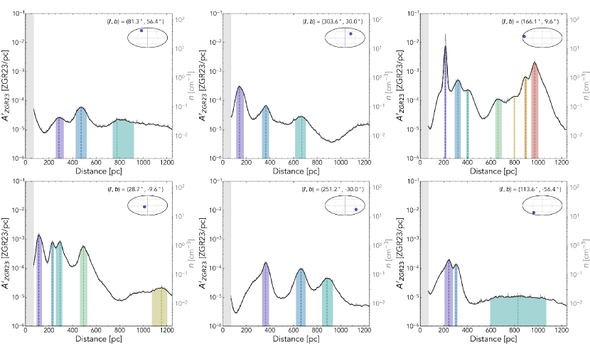
Figure 1: Differential dust extinction in the E23 map ($A^{\prime}_{ZGR23}$) as a function of distance, along six representative lines of sight. The raw E23 extinction is shown in gray and the smoothed extinction is shown in black. Peaks identified in the dust map are shown by the colored shaded regions, with peak distance $d_{peak}$ marked by a dashed line and peak shading extending from $d_{inner}$ to $d_{outer}$. The first peak along the LOS (corresponding to the shell of the Local Bubble) is always shaded in purple. The inner $d<69$ pc region where the E23 map is undefined is shaded in gray. The secondary y-axis shows the conversion from $A^{\prime}_{ZGR23}$ to volume density $n$. The inset Mollweide projection shows the position of each LOS on-sky.

We define the Local Bubble’s shell as the first significant peak in extinction along the LOS from the Sun. We define a peak as local maximum along the LOS with a prominence greater than some given value (where “prominence” is the height of the peak above its base) . Our technique is predicated on the idea that the vacuous inner cavity of the Local Bubble is bounded by a denser shell of neutral gas and dust; however, as we will discuss in §2.3.1, our methodology is insensitive to the precise density of the shell.

We smooth the LOS extinction profile using a Gaussian kernel with $\sigma_{smooth}=7$ pc to reduce the effects of noise in our peak detection, and require a minimum peak prominence of $P_{min}=2.04\times 10^{-6}$ ZGR23/pc. We describe the selection of these parameters in Appendix A. We identify peaks using the python package scipy’s find_peaks function.

We define the inner and outer edges of each peak as the distance before ($d_{inner}$) and distance after ($d_{outer}$) the peak at which the differential extinction $A^{\prime}_{ZGR23}$ is equal to

$$A^{\prime}_{0.5}=A^{\prime}_{peak}-0.5P,$$ (2)

i.e., the peak height minus half the peak prominence. If the half prominence boundaries contain a separate but lower prominence peak, we adjust the inner (or outer) edge of the overlapping peak to fall at the local minimum between the two peaks. We additionally derive and report the inner and outer edges (and all other associated properties of our Local Bubble model) at a more generous threshold of $A^{\prime}_{0.9}$. We define the thickness of a given peak as $\Delta_{peak}=$ $d_{outer}$ $-$ $d_{inner}$, and require a minimum thickness (at $A^{\prime}_{0.5}$) of 3 pc so that $d_{inner}$ $\neq d_{peak}\neq$ $d_{outer}$.

Six representative LOS with identified peaks are shown in Figure 1. Wide variations in peak shape, width, and height are present across the sky.

We first performed our peak finding method on the full E23 map out to $d=1244$ pc. For the vast majority of LOS, the first peak along the LOS was within a distance of $d=650$ pc, with only 23 (0.003%) isolated LOS at high latitudes having peak distances beyond $d=650$ pc. We interpret these isolated LOS as being unassociated with the Local Bubble and, for our final model of the Local Bubble, performed our peak finding method on the E23 map truncated to $d=650$ pc to exclude these handful of LOS well beyond the surface of the Local Bubble.

2.3 Derived Peak Properties

Table 1: Properties of the Local Bubble’s Shell

Property	Symbol	Minimum	P2.28	Median	P97.72	Maximum	Units
Inner Edge	$d_{inner}$	69	80	150	322	592	pc
Peak Distance	$d_{peak}$	71	91	170	362	616	pc
Outer Edge	$d_{outer}$	72	101	191	395	633	pc
Thickness	$\Delta_{shell}$	3	13	35	123	357	pc
Peak Density	$n_{peak}$	0.02	0.04	0.61	21	770	cm-3
Extinction	$A_{G}$	<0.001	0.002	0.02	0.34	2.8	mag
Inclination	$\gamma$	0	4	25	63	90	$\degree$

Note. — P_i denotes the $i$-th percentile of the distribution. Under a normal distribution, P_2.28 and P_97.72 represent the $\mp 2\sigma$ intervals, respectively. See Figure 7 for a graphical representation of these distributions.

For each LOS, we calculate various properties of the Local Bubble’s shell, including extinction, density, mass, and inclination to the plane-of-the-sky.

2.3.1 Extinction, Density, and Mass

For a peak along the LOS extending over $i$ distance slices between $d_{inner}$ $\leq d\leq$ $d_{outer}$, integrated extinction can be calculated as the sum of unsmoothed differential extinction,

$$A_{ZGR23}=\sum_{i}A^{\prime}_{ZGR23,i}dr_{i},$$ (3)

where $dr_{i}=1$ pc for all slices. ZGR23 extinction can be converted to Gaia G-band extinction $A_{G}$ (centered at $\lambda=673$ nm, Jordi et al., 2010) using ZGR23’s published extinction curve,

$$A_{G}=2.0407A_{ZGR23}.$$ (4)

We report the integrated $A_{G}$ for each LOS. We emphasize that uncertainties (calculated as in §2.3.3) on extinctions below $A_{G}\simeq 0.005$ mag are generally very high (with distance uncertainties typically $\gtrsim 50$ pc).

The total volume density of hydrogen nuclei $n$ within each of the $i$ distance slices along a given LOS can be derived from extinction by following Zucker et al. (2021) in assuming the ratio of hydrogen column density to extinction is constant ($A_{G}/N_{H}\simeq 4.0\times 10^{-22}$ cm² mag, Draine 2003, 2009), leading to a relationship

$$\begin{split}n_{i}&=\frac{1}{(A_{G}/N_{H})}\left(\frac{dA_{G,i}}{1\textrm{pc}}\right)\frac{da_{i}\ dr_{i}}{dv_{i}}\\ &=1653\ \textrm{cm}^{-3}\ A^{\prime}_{ZGR23,i},\end{split}$$ (5)

where $da_{i}$ is the projected physical area of the pixel in distance slice $i$, $dr_{i}$ is the radial separation between slice $i$ and $i+1$, and $dv_{i}=da_{i}dr_{i}$ is the volume spanned between slice $i$ and $i+1$. We summarize the derivation of this relationship in Appendix D. For each LOS, we report the maximum unsmoothed density, $n_{peak}$, reached between $d_{inner}$ and $d_{outer}$. We additionally provide an interpolated 3D grid (in heliocentric Cartesian x-y-z space) of dust in the Local Bubble’s shell.

When integrated over the $i$ slices between $d_{inner}$ $\leq d\leq$$d_{outer}$, volume density yields mass contained in the peak,

$$M=1.37\ m_{p}\sum_{i}\ n_{i}\ dv_{i},$$ (6)

where $m_{p}$ is the mass of a proton and 1.37 is a factor derived from cosmic abundances to convert from hydrogen mass to total mass including helium. To calculate $dv_{i}$, we approximate $da_{i}\simeq d_{i}^{2}\theta^{2}$, where $d_{i}$ is the distance to slice $i$ and $\theta^{2}$ is the area of the HEALPix pixel (which at $N_{\rm{side}}={256}$ is equal to $\theta^{2}\simeq 1.6\times 10^{-5}$ rad²). Radial separation is equal to $dr_{i}=1$ pc for all slices.

2.3.2 Inclination

The angle of the Local Bubble’s shell to the plane-of-the-sky (POS), or the shell’s inclination, may be a significant factor in observations of e.g., cosmic ray deflection, pulsar scintillation, polarization fractions, and other similar quantities measured from our vantage point in the Solar System (see e.g. Ocker et al., 2024). We estimated the inclination of the Local Bubble’s shell (at $d=d_{peak}$) for each LOS by fitting a tangent plane via singular value decomposition (SVD) to its 500 nearest neighboring peaks in 3D Cartesian space (including the central point, and with neighborhoods typically spanning a space 5–25 pc in radius).

Specifically, for each LOS and collection of neighbors we perform SVD as implemented in the python package numpy (Harris et al., 2020), where decomposition is performed as $A=U\Sigma V^{T}$, where $A$ is a 3$\times$500 matrix of point positions (with coordinates shifted to an origin at their mean position), $U$ is a 3$\times$3 matrix with columns $(\bf{u}_{1},\bf{u}_{2},\bf{u}_{3})$, $V$ is a 500$\times$500 matrix with columns $(\bf{v}_{1},...,\bf{v}_{500})$, and $\Sigma$ is a diagonal matrix with the singular values of $A$ as the diagonal entries, $\sigma_{i}=\Sigma_{ii}$. The normal vector to the tangent plane, $\textbf{n}=(n_{x},n_{y},n_{z})$, can then be extracted as the third left singular vector, $\textbf{n}=\bf{u}_{3}$.

The angle between the Local Bubble’s surface and the POS can then be defined as the angle between n and the LOS (the normal to the POS),

$$\gamma=\arccos(\textbf{n}\cdot\textbf{e}_{L}),\rm{\ \ }\gamma\in[0\degree,90\degree],$$ (7)

where $\textbf{e}_{L}$ is the normalized LOS (a unit vector from the Sun to the Local Bubble’s surface, $\textbf{e}_{L}=(x/d,y/d,z/d)$).

2.3.3 Uncertainties

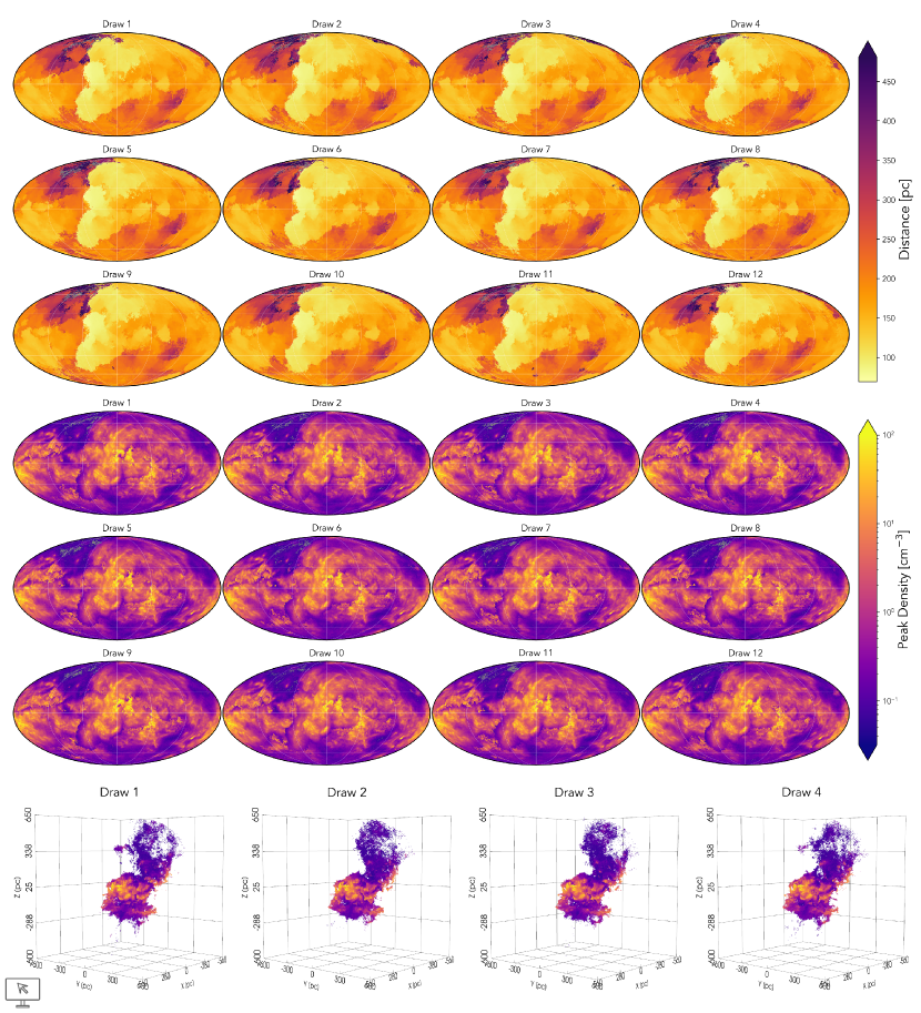
Figure 12: Top rows: Mollweide projections of distance to the first peak along the LOS in each of the 12 draws of the E23 map are shown. Center rows: As top, but for peak density. Bottom row: 3D views of models derived from draws 1, 2, 3, & 4, colored by peak density. Interactive 3D figure showing all 12 draws: https://theo-oneill.github.io/localbubble/draws/. To animate the figure, click "Play loop" in the interactive control panel.

We estimate statistical uncertainties on our derived peak properties by applying our peak finding method to each of the 12 draws of the E23 map (with results described in Appendix B, and Figure 12 showing projected 2D and interactive 3D views of the Local Bubble model derived from each draw). Uncertainties along each LOS are then defined as the standard deviation of the draw-derived properties. We report uncertainties for all quantities except on-sky position and derived Cartesian coordinates.

We estimate the uncertainty on the total mass of the Local Bubble’s shell in two parts: 1) the statistical uncertainty as the standard deviation of the total masses in each draw, and 2) the systematic uncertainty as the uncertainties introduced by A) our procedure for defining peak edges (affecting the total extinction $A_{G}$ contributed by the shell) and B) our conversion from extinction to mass (affecting the factor $A_{G}/N_{H}$).

We expect the bulk of the uncertainty stemming from A) is contributed by the size of the smoothing kernel applied to differential extinction along the LOS, $\sigma_{smooth}$; shell thickness increases with smoothing scale, which in turn increases shell extinction and mass estimates. To quantify this effect, we calculated the total mass of the Local Bubble’s shell $M_{shell}(\sigma_{smooth})$ for smoothing scales between $\sigma_{smooth}=3$ pc and $\sigma_{smooth}=10$ pc (using the same fiducial $P_{\rm{min}}$ for all $\sigma_{smooth}$). We performed ordinary least squares regression to estimate the slope of the relationship between smoothing kernel size and the percent difference between $M_{shell}(\sigma_{smooth})$ and the fiducial $M_{shell}(7\ \textrm{pc})$, defined as $\delta M_{shell}=[M_{shell}(\sigma_{smooth})-M_{shell}(7\ \textrm{pc})]/[M_{shell}(7\ \textrm{pc})]$. We find that, for an increase in $\sigma_{smooth}$ of 1 pc, $\delta M_{shell}$ will on average increase by 5.8$\%\pm 0.1\%$. Standard diagnostics of the fit suggest this model is adequate at predicting $\delta M_{shell}$ (coefficient of determination $R^{2}=0.998$, $F$-test statistic of $F=3941$ with $p<0.001$). We use this factor as a proxy for the systematic uncertainty on shell mass stemming from A).

We estimate the uncertainty from B) by using the simplifying assumption that the majority of the uncertainty is introduced by the assumption of a fixed reddening vector $R_{V}$ used to derive the relationship between $A_{\lambda}/N_{H}$ by Draine 2003. Our adopted $A_{G}/N_{H}\simeq 4.0\times 10^{-22}$ cm² mag was calculated using the relationships derived by Draine (2003) for a fixed $R_{V}=3.1$ (Cardelli et al., 1989); if instead $R_{V}=2.8$ or $R_{V}=3.2$ were assumed (the range within which ZGR23’s derived extinction curve is consistent with Cardelli et al. 1989), factors of $A_{G}/N_{H}\simeq 3.5\times 10^{-22}$ cm² mag or $A_{G}/N_{H}\simeq 4.1\times 10^{-22}$ cm² mag, respectively, would result. We use this $\sim$10% variation as a proxy for the uncertainty on $A_{G}/N_{H}$.

Total shell mass is proportional to the product of integrated $A_{G}$ (which is influenced by smoothing scale) and the conversion factor $A_{G}/N_{H}$. We expect these quantities to vary independently, so we estimate our total systematic uncertainty on total shell mass by adding our fractional uncertainties in quadrature, leading to a systematic uncertainty on $M_{shell}$ of order 12%.

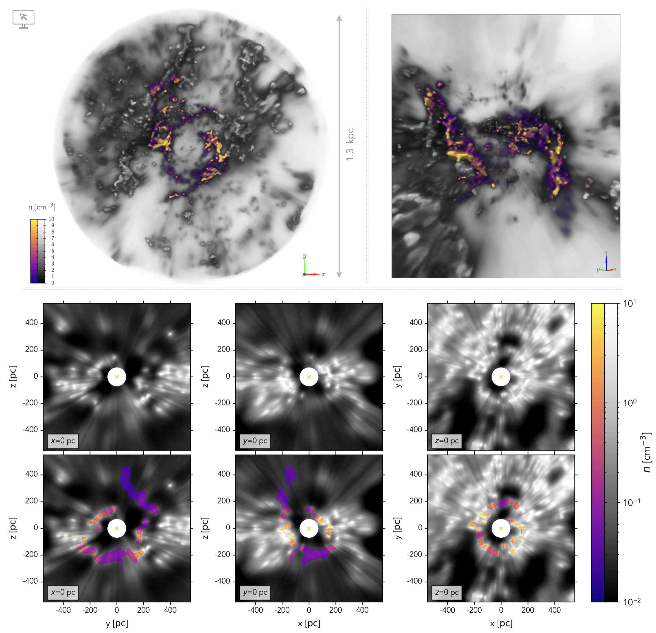
Figure 2: Dust in the E23 map identified as being part of the Local Bubble’s shell is shown in 3D (top) and 2D projections (bottom). Top Row: Two views of the 3D interactive figure. The E23 map is shown in grayscale (for $d\leq 650$ pc, with [5 pc]³ voxels), and Local Bubble shell dust is highlighted in color (with [2 pc]³ voxels, smoothed with a Gaussian beam of $\sigma=2$ pc for visualization purposes). Center & Bottom Rows: 2D slices through the E23 volume are shown, with slices along the $x=0$ pc (left), $y=0$ pc (center), and $z=0$ pc (right) planes. Center row shows only the E23 map, bottom row shows the E23 map with Local Bubble shell dust overlaid in color. Both the full map and shell dust are shown with [2 pc]³ voxels. Color maps are scaled linearly in the 3D figure and logarithmically in the 2D figures. Interactive 3D figure: https://theo-oneill.github.io/localbubble/shell_dust/

3 Results

3.1 Properties of the Local Bubble’s Shell

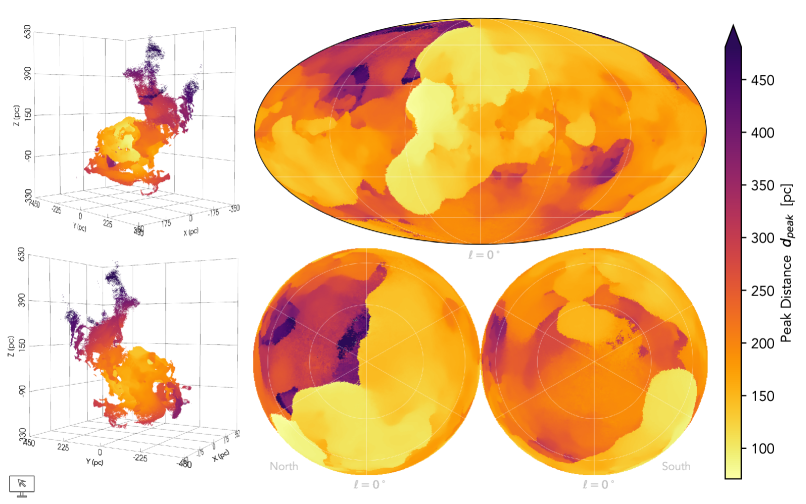
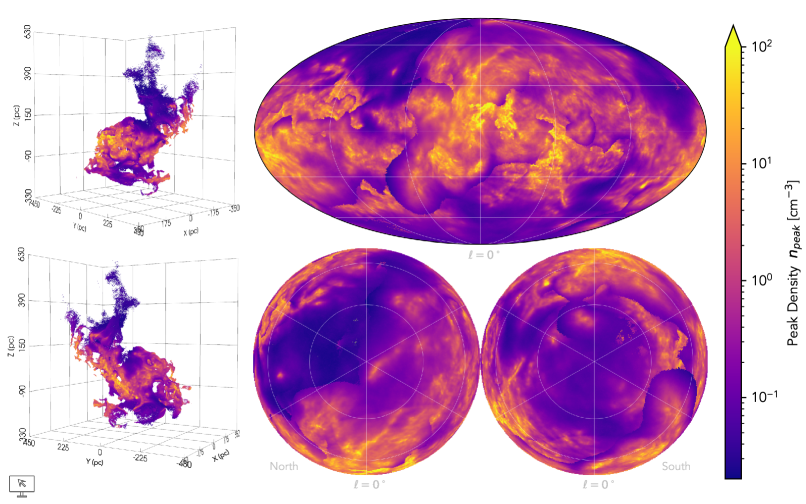
Figure 3: Distance to the peak extinction surface of the Local Bubble, $d_{peak}$, shown in 3D (left column) and 2D Mollweide (top right) and 2D polar (North: bottom center, South: bottom right) projections. Interactive 3D figure is available at: https://theo-oneill.github.io/localbubble/distance/

Figure 4: Peak density of dust in the Local Bubble’s shell, $n_{peak}$, in 3D and 2D projections. Interactive 3D figure: https://theo-oneill.github.io/localbubble/density/

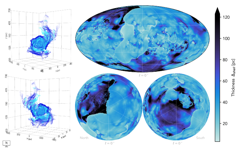
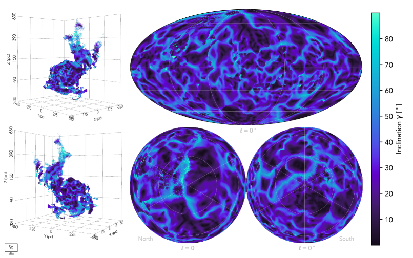
Figure 5: Thickness of the Local Bubble’s shell, $\Delta_{shell}$, in 3D and 2D projections. In 3D, the inner surface is shown by the light blue points and the outer surface by the dark blue points. Interactive 3D figure: https://theo-oneill.github.io/localbubble/thickness/

Figure 6: Inclination of the Local Bubble’s shell to the plane-of-the-sky, $\gamma$, in 3D and 2D projections. Interactive 3D figure: https://theo-oneill.github.io/localbubble/inclination/

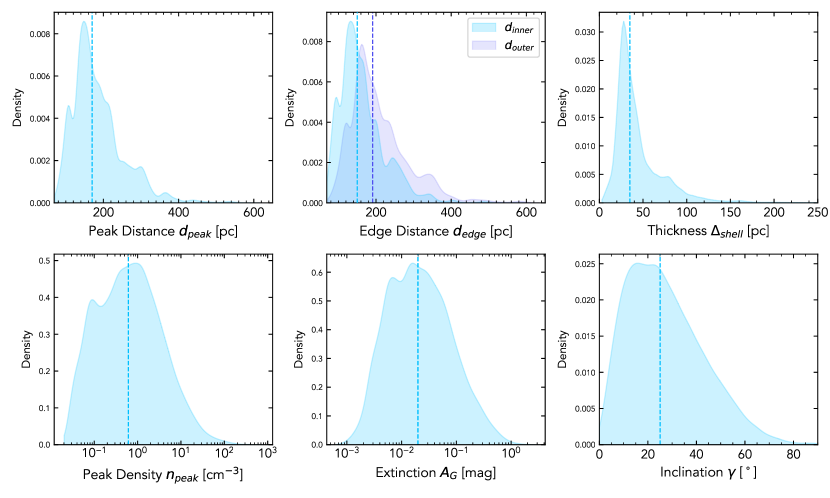
Figure 7: Kernel density estimations of Local Bubble shell properties. Top, from left: peak distance $d_{peak}$; inner and outer edge distances $d_{inner}$ and $d_{outer}$; thickness $\Delta_{shell}$. Bottom, from left: peak density $n_{peak}$; extinction $A_{G}$; inclination to the POS $\gamma$. In all panels, the median of the distribution is marked by a dashed vertical line.

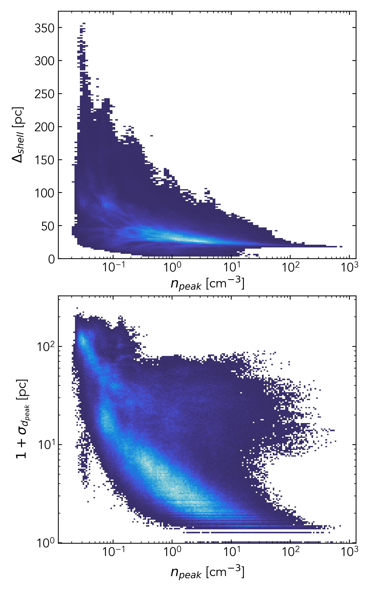
Figure 8: 2D histograms of shell peak density $n_{peak}$ vs. (top) shell thickness $\Delta_{shell}$, and vs. (bottom) peak distance uncertainty $\sigma_{d_{peak}}$ (plotted as $1+\sigma_{d_{peak}}$ to allow a logarithmic scale without excluding LOS with $\sigma_{d_{peak}}=0$ pc).

Dust identified as being a part of the Local Bubble’s shell by our peak-finding procedure is highlighted in color in Figure 2 in interactive 3D form and in 2D slices through the $x=0$ pc, $y=0$ pc, and $z=0$ pc planes; the rest of the E23 map is shown in grayscale. Various properties of the Local Bubble’s shell are shown in 2D projection and 3D interactive form in the subsequent figures. Distance from the Sun to the peak extinction surface of the Local Bubble, $d_{peak}$, in shown in Figure 4, and peak shell density, $n_{peak}$, is shown in Figure 4. Shell thickness, $\Delta_{shell}$, (at $A^{\prime}_{0.5}$) is shown in Figure 6, and shell inclination to the POS, $\gamma$, is shown in Figure 6. Uncertainties on peak distance, $\sigma_{d_{peak}}$ are shown in Appendix B’s Figure 13. The statistical distributions of the shell’s properties are summarized in Table 1 and shown graphically in Figure 7.

Our model of the Local Bubble’s shell is extremely irregular and asymmetric, with wide variations in morphology and peak properties present over the surface of the Bubble. At low altitudes, the shape of the Local Bubble is roughly spherical, but is marked by many small scale discontinuities and extensions. At higher altitudes, a large scale, asymmetric region of increased distances and decreased densities is present towards Galactic North; we discuss this feature (which we associate with representing a Chimney out of the Galactic plane) in §4.1. The Local Bubble’s shell is much more extended in the $y$ and $z$ directions than in $x$, spanning the coordinates $-300\leq x\leq 330$ pc, $-355\leq y\leq 445$ pc, and $-300\leq z\leq 600$ pc. The geometric center of the Local Bubble’s shell is located at $(x,y,z)=(-9.8\pm 0.3,1.9\pm 0.3,0.2\pm 0.8)$ pc, although we caution that our peak-finding method extending radially outward from the Sun’s position at $(x,y,z)=(0,0,0)$ pc likely influences this result.

Various correlations exist between properties of the Local Bubble’s shell. As shown in Figure 8, thickness and peak density are moderately negatively correlated (Spearman $\rho_{s}=-0.61$, $p<0.001$), with thicker shell sections generally having lower peak densities. Uncertainties on distance to the shell’s surface are also moderately negatively correlated with peak density ($\rho_{s}=-0.66$, $p<0.001$), with denser structures having lower distance variability between draws of the E23 map.

We find a total dust-traced mass in the Local Bubble’s shell of $M_{shell}=(6.0\pm 0.7\ (\textrm{systematic})\pm 0.1\ (\textrm{statistical}))\times 10^{5}\ M_{\odot}$ at an edge threshold of $A^{\prime}_{0.5}$. As described in §2.3.3, this quantity depends strongly on the size of the smoothing kernel applied along the LOS; for $\sigma_{smooth}=6$ pc, $M_{shell}=5.6\times 10^{5}\ M_{\odot}$, while for $\sigma_{smooth}=8$ pc, $M_{shell}=6.3\times 10^{5}\ M_{\odot}$. At a more generous threshold of $A^{\prime}_{0.9}$, the total mass (for the fiducial $\sigma_{smooth}=7$ pc) is $M_{shell}=8.0\times 10^{5}\ M_{\odot}$. These estimates include the dust-traced mass of a number of nearby molecular clouds (discussed further in §4.3). At all thresholds, this shell mass measurement is smaller than Zucker et al. (2022)’s estimate of $M_{shell}=(1.4\pm 0.6)\times 10^{6}\ M_{\odot}$ derived from the Pelgrims et al. (2020) model of the Local Bubble (assuming a typical shell thickness of 50–150 pc) using the Leike et al. (2020) 3D dust map. We attribute this difference to the decreased thickness of the Local Bubble in our new model, enabled by the increased spatial resolution of the E23 dust map.

3.2 Properties of the Local Bubble’s Interior

We additionally derive several relevant characteristics of the interior of the Local Bubble (defined for our purposes as $d<d_{inner}(A^{\prime}_{0.9})$). The Local Bubble’s interior covers a volume of $1.9\times 10^{7}$ pc³ (including the $d<69$ pc sphere that the E23 map does not probe), which is equivalent to a sphere with a radius of $R=$165 pc.

The volume density of dust within the Local Bubble’s interior (excluding the inner $d<69$ pc region) spans a $\mp 2\sigma$ interval from $n=0.005$ cm^-3 to $n=0.35$ cm^-3, with a median of $n=$0.02 cm^-3. This median density of $n=$ 0.02 cm^-3 is roughly consistent with the predicted density derived from the pulsar dispersion measure. Linsky & Redfield (2021) find a typical electron density of $n_{e}=0.0120\pm 0.0029$ cm^-3 for lines of sight towards the nearest five pulsars from the Sun, lying at distances of 156-372 pc. Assuming the Local Bubble’s interior is fully ionized ($n_{e}=n_{H}^{+}$), the volume density of hydrogen nuclei $n$ we derived in Eqn. 5 would be equal to $n_{H}^{+}$, so our derived density agrees with the density predicted by the pulsar dispersion measure to within a factor of two.

Along each LOS, the ratio of the minimum dust density in the Local Bubble’s interior, $n_{min,interior}$, to the peak dust density in the Local Bubble’s shell, $n_{peak}$, spans a $\mp 2\sigma$ interval from $n_{peak}/n_{min,interior}=$2 to 800, with a median ratio of $30$. The ratio between the interior and shell dust density is lowest along the Northern Chimney feature and along the diffuse edges of the lower-latitude shell.

4 Discussion

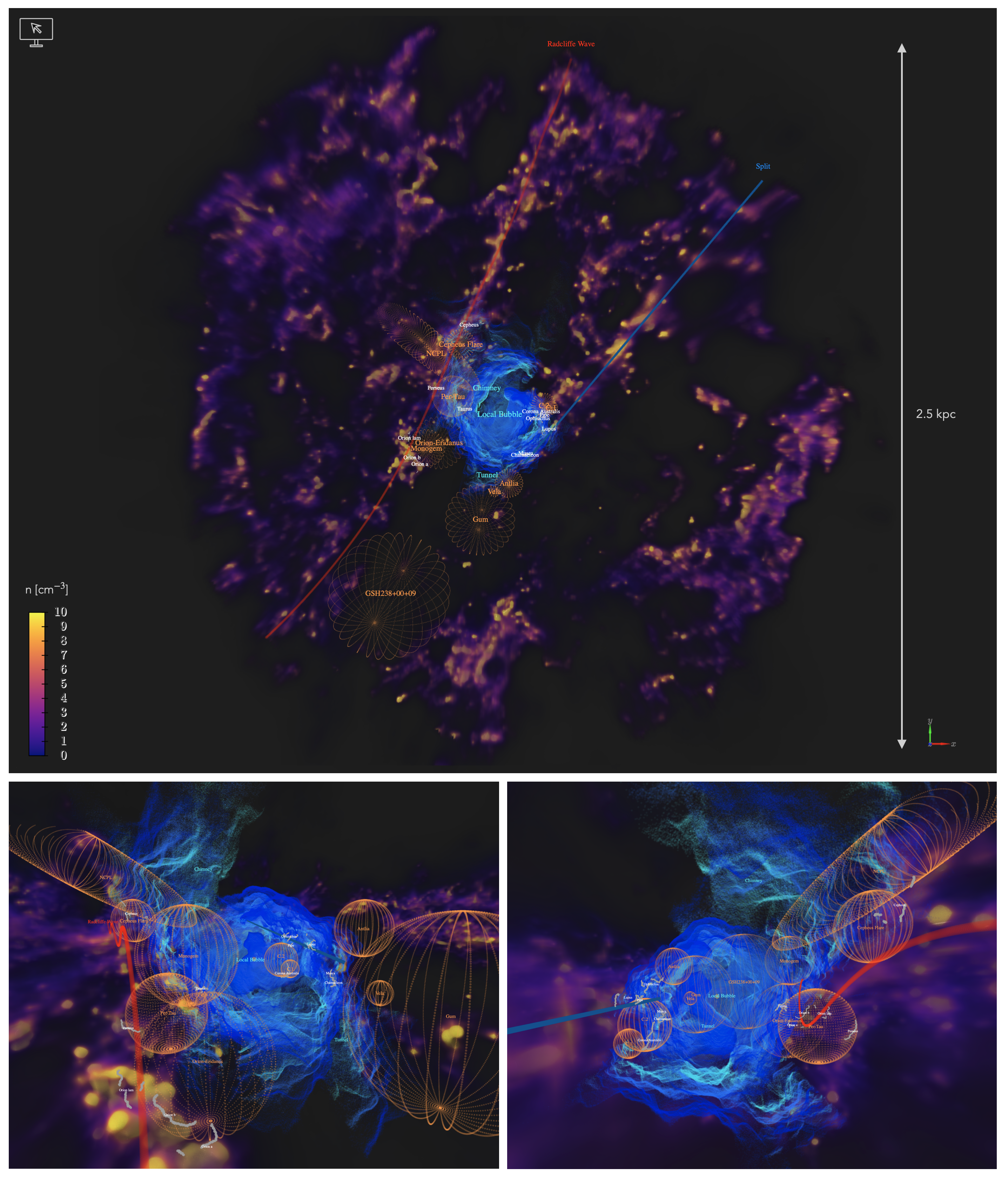
Figure 9: A 3D interactive view of the Local Bubble in the context of the Solar Neighborhood. The inner, peak, and outer edges of the Local Bubble’s shell are shown in light blue, medium blue, and dark blue, respectively. Structures in the Solar Neighborhood (including 3D dust, nearby bubble and shells, molecular clouds, and other Galactic features) are summarized in Table 2. Interactive 3D figure: https://theo-oneill.github.io/localbubble/neighborhood/

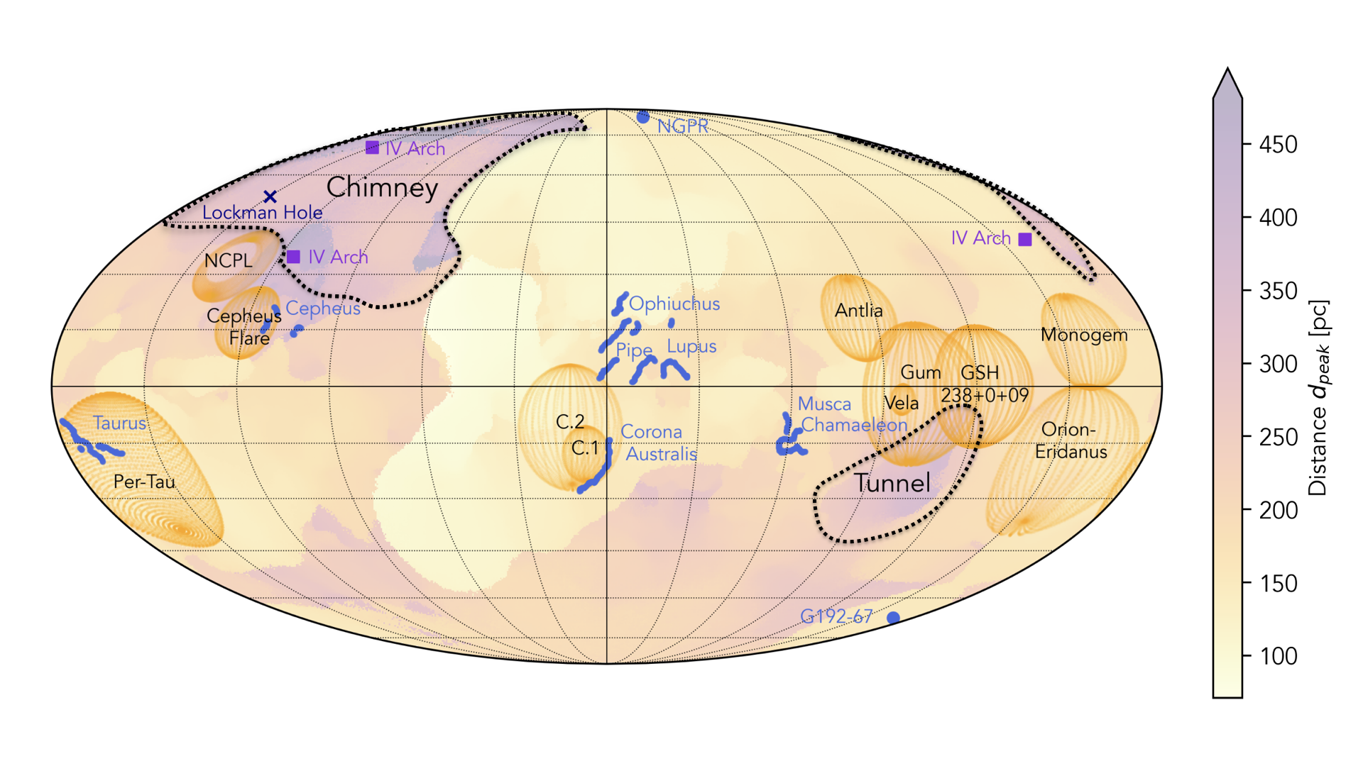
Figure 10: A 2D view of structures in the Solar Neighborhood that may be relevant to the Local Bubble’s evolution. This includes nearby bubbles and shells (orange), molecular clouds and dust features (blue), and other features of the 2D sky discussed in text. Distance to the Local Bubble’s shell (Fig. 4) is shown in the background. Approximate outlines of the “Chimney” and “Tunnel” features are shown by the black dotted contours, and are drawn by eye based on shell distance and density.

Table 2: Structures in the Solar Neighborhood

Object Type	Name	Notes	Reference
Local Bubble	Local Bubble Model	Peak Density, Inner & Outer Edges	This work
Dust	3D Dust Map	Downsampled to (10 pc)3 voxels	Edenhofer et al. (2023)
Molecular Clouds	Cloud Skeletons	Cepheus, Chamaeleon, Corona Australis, Lupus,	Zucker et al. (2021)
		Musca, Ophiuchus, Orion, Perseus, Pipe, Taurus
Galactic Structures	Radcliffe Wave		Konietzka et al. (2024)
	Splita		Lallement et al. (2019)
Shells & Cavities	Per-Tau Shell	(x, y, z, R) = (-190, 65, -84, 78) pc	Bialy et al. (2021)
	NCPL	Prolate Spheroid	Marchal & Martin (2023)
	Antlia SNR	($\ell$, $b$, $d$, D) = (275.5$\degree$, 18.4$\degree$, 250 pc, 23$\degree$)	Fesen et al. (2021)
	C.1 Shellb	($\ell$, $b$, $d$, D) = (7$\degree$, -18$\degree$, 190 pc, 15$\degree$)	Bracco et al. (2020)
	C.2 Shellb	($\ell$, $b$, $d$, D) = (12$\degree$, -11$\degree$, 160 pc, 33$\degree$)	Bracco et al. (2020)
	Cepheus Flare Shell	($\ell$, $b$, $d$, D) = (120$\degree$, 17$\degree$, 300 pc, 19$\degree$)	Olano et al. (2006)
	Gum Nebula	($\ell$, $b$, $d$, D) = (258$\degree$, -2$\degree$, 400 pc, 36$\degree$)	Sushch et al. (2011)
	GSH238+00+09	($\ell$, $b$, $d$, D) = (238$\degree$, 0$\degree$, 790 pc, 32$\degree$)	Heiles (1998)
	Monogem Ring	($\ell$, $b$, $d$, D) = (203$\degree$, 12$\degree$, 300 pc, 25$\degree$)	Knies et al. (2018)
	Orion-Eridanus	($\ell$, $b$, $d$, D) = (205$\degree$, -20$\degree$, 290 pc, 40$\degree$)	Pon et al. (2016)
	Vela SNR	($\ell$, $b$, $d$, D) = (264$\degree$, -3.4$\degree$, 290 pc, 8$\degree$)	Sushch et al. (2011)

Note. — The models of the Per-Tau Shell and the NCPL were derived from 3D dust maps. The other shells’ centers are estimated from 2D data and projected to 3D based on assumed distances $d$ and on-sky diameters $D$.

^a The linear model of the Split is placed by eye as it agrees with the E23 map at a uniform altitude of $z=0$ pc, and is intended only to guide the viewer to the relevant dust feature.

^b The distances derived for the C.1 and C.2 shells by Bracco et al. (2020) ($d=186$ pc and $d=144$ pc, respectively) were measured at the edges of the shells as viewed in 2D projection; in this work, we place the shells’ centers at estimated distances that are one solution geometrically consistent with the measured distances to the shell edges.

We provide a 3D interactive view of the Local Bubble in the context of the Solar neighborhood in Figure 9. Our model of the Local Bubble is represented through its inner and outer edges, as well as position of peak extinction along the LOS. Structures represented in this figure are listed in Table 2 and discussed throughout this section; a subset of structures that may be adjacent to the Local Bubble’s surface are shown in 2D projection in Figure 10.

We highlight several features of our new model of the Local Bubble:

4.1 A Local Chimney

The most prominent feature of our new model is that the Northern cap of the Local Bubble appears partially open, being marked by a region of particularly distant ($d=$300–600 pc) and low-density dust. This open cap spans about $\frac{1}{3}$ of the high latitude ($b>30\degree$) Northern sky, extending over the range of $\ell\simeq$ ($60^{\degree}$ – $190^{\degree}$) and $b\gtrsim 30^{\degree}$. The density of material in this feature is the lowest over the entire sky as we have estimated it (typically $\sim 10^{-1.5}$ cm^-3). Shell thickness is also extremely high (>100 pc). In 3D space, this region of extremely low density dust spans altitudes of $z\simeq 150$ pc to $z\simeq 600$ pc (although we emphasize that distance and, correspondingly, altitude uncertainties are generally very large in this region as a result of the low densities being probed).

Early 3D maps of the Local Bubble (e.g., Sfeir et al., 1999; Welsh et al., 1999; Vergely et al., 2001; Lallement et al., 2003) proposed that the Local Bubble was a Local Chimney, with tilted, open caps to both the North and South. More recent models of the Local Bubble made with intermediate-resolution dust maps (Pelgrims et al., 2020) have found that the Northern and Southern caps both appeared closed. The distant, low-density Northern dust feature in our new model appears morphologically consistent with supporting the earlier view of a Local Chimney extending from the Local Bubble into the lower Galactic halo. The tilt of the Northern Chimney in our model of the Local Bubble (centered roughly towards $(\ell,b)=({120}\degree,{60}\degree)$) is similar but not identical to the tilt found in those earlier Local Chimney maps like that of Lallement et al. (2003), who reported a tilt centered towards $(\ell,b)=({180}\degree,{70}\degree)$.

Unlike the earlier maps, we find a closed surface across the Southern cap of the Local Bubble. This surface appears relatively cohesive and traces a nearly flat 3D surface comprised of dust that is generally higher density ($\simeq 10^{-1}$ cm^-3) than the tenuous Northern material (but is still lower density than the bulk of the lower latitude shell). Uncertainties on distance to this material are much lower than in the low density Northern material, and thickness and shell inclination are generally more consistent between adjacent LOS than in the North. This suggests that the Southern cap is closed, and that the Local Bubble is an asymmetric Local Chimney.

An asymmetric Local Chimney presents interesting implications for the past and present evolution of the Solar Neighborhood. Simulations and theory suggest that superbubbles like the Local Bubble are only able to break out of the denser gas in the disk and form chimneys and fountains reaching into the Galactic halo under specific conditions; the stratified distributions of gas density, magnetic field orientation & strength, and related factors are expected to play large roles in inhibiting or encouraging superbubble blowout, as are the positions of a bubble’s progenitor supernovae relative to the midplane of the disk (e.g., Mac Low & McCray, 1988; Mac Low et al., 1989; Ferriere et al., 1991; Koo & McKee, 1992; Tomisaka, 1998; Korpi et al., 1999; de Avillez & Berry, 2001; de Avillez & Breitschwerdt, 2005; Baumgartner & Breitschwerdt, 2013; Walch et al., 2015; Girichidis et al., 2016; Fielding et al., 2017; Kim et al., 2017; Fielding et al., 2018; Kim & Ostriker, 2018; Orr et al., 2022a, b).

Assuming the Galactic midplane falls somewhere between $z\simeq$ -25 to -5 pc (e.g., Maíz-Apellániz, 2001b; Jurić et al., 2008; Anderson et al., 2019, relative to the Sun’s position and IAU midplane at $z=0$ pc), the vertical extrema of the Bubble falls $>$600 pc above the midplane in the North and $>$270 pc below the midplane in the South. The scale height of $\textrm{H}\scriptstyle\mathrm{I}$ gas in Milky Way-like galaxies is expected to flare with galactocentric radius and be of order a few hundred parsecs near the position of the Sun (Bacchini et al., 2019; Patra, 2020; Gensior et al., 2023), placing the Northern extremes of the Local Chimney in the lower halo. We caution that the high uncertainty, low density dust found in this region should not be interpreted as a definitive detection of an upper boundary or “end” of the Northern Local Chimney.

The observed asymmetric Local Chimney suggests that either the physical conditions in the Galactic Northern and Southern hemispheres were significantly different from each other before the expansion of the Local Bubble, or that the Local Bubble’s progenitor (or even only most recent) SN were preferentially located in the North, above the Galactic midplane. Blow out in the South might then have been halted by encountering the denser gas in the plane, while blow out in the North would have been able to proceed due to a lack of interference. The Sco-Cen association is a strong candidate for hosting the progenitor clustered supernovae that launched the initial expansion of the Local Bubble (as proposed by, e.g., Maíz-Apellániz, 2001a; Fuchs et al., 2006; Breitschwerdt et al., 2016); stellar tracebacks calculated by Zucker et al. (2022) place clusters in the association at heights of only $z=$ -16 to -17 pc when the Bubble was born $\sim$14 Myr ago, roughly consistent with the height of the present-day midplane.

In their analytic modeling of the effects of clustered supernovae on bubble evolution, Orr et al. (2022b) draw a distinction between superbubbles that simply coast out of the disk (meaning that the production of the supernovae powering a bubble’s expansion has ceased by the time the bubble reaches the disk scale height) vs. those whose breakout is powered by ongoing supernovae. They find that coasting superbubble breakout should be extremely difficult to achieve under typical conditions of disk galaxies like the Milky Way. In this context, the apparent bursting morphology of the Local Bubble suggests that the Local Chimney was formed from the Local Bubble under the power of ongoing supernovae – although we note the time and position of the most recent supernovae in the Local Bubble is uncertain, and the interval elapsed since the Local Bubble formed a chimney is unknown.

A Local Chimney extending from the Local Bubble would additionally have implications for the present-day conditions in the interior of the Local Bubble, especially temperature and pressure, as chimneys are expected to play a key role in dissipating the hot interiors of feedback-driven bubbles. Initial evidence for a hot Local Bubble has faced challenges in recent years (e.g., Welsh & Shelton, 2009; Linsky & Redfield, 2021), and a chimney venting the initially hot Bubble interior into the lower halo could provide a path to a resolution of this long standing issue. However, the degree to which mixing and cooling could have occurred would directly depend on the timescale of the Local Bubble’s breakout and formation of a chimney, which at present is unconstrained.

4.1.1 Connection to Intermediate Velocity Clouds?

In addition to allowing the hot interior of superbubbles to be dissipated, chimneys from burst superbubbles are theorized to lead to the creation of populations of intermediate velocity clouds (IVCs) contributing to a galactic fountain flow. In this model, IVCs are posited to be fragments of burst superbubbles that were launched into the lower Galactic halo, before cooling and raining back down onto the Galactic plane — propagating a galactic fountain and leading to new star formation and the distribution of metals throughout the ISM (Shapiro & Field, 1976; Bregman, 1980).

If the Local Bubble is only open to the North as found in our new model, one might expect to observe a higher number of IVCs in the North than the South, with distinctions arising both chemically and kinematically between the populations of IVCs. Such an asymmetry between the Northern and Southern distributions of IV gas is well known, with a number of studies having found significant differences in the distribution of IVCs between hemispheres. Much of this asymmetry is driven by large Northern complexes of IV gas with negative radial velocities known as the IV Arch, IV Spur, and low latitude IV Arch (Kuntz & Danly, 1996). These features are easily observable in observations of IV 21 cm emission in the Northern vs. Southern hemispheres (e.g., as compiled by Albert & Danly, 2004; Wakker, 2004); the IV Arch in particular stretches from approximately $(\ell,b)=({115}\degree,{35}\degree)$ to $(\ell,b)=({150}\degree,{70}\degree)$ to $(\ell,b)=({200}\degree,{40}\degree)$ (Kuntz & Danly, 1996), as shown by reference points in Figure 10.

Statistical analyses of the Northern vs. Southern IVC populations have confirmed the asymmetries visible by eye. Röhser et al. (2016) found a strong asymmetry in the number of high-latitude ($|b|\geq 20\degree$) IVCs with molecular gas content in the Northern vs. Southern hemispheres, with the North having 3.6$\times$ the number of molecular IVCs detected in the South. Panopoulou & Lenz (2020) similarly observed a very strong asymmetry in the total number of IVCs along each LOS in the North vs. South (on average, 3 clouds per HEALPix pixel in the North vs 2.5 clouds per pixel in the South), as assessed via Gaussian decomposition of high latitude ($|b|\geq 30\degree$) $\textrm{H}\scriptstyle\mathrm{I}$ line data compiled by the HI4PI survey (HI4PI Collaboration et al., 2016). Many of these observed statistical asymmetries are in part driven by the presence of the IV Arch and adjacent IV gas.

We observe a correspondence between the on-sky position of the IV Arch (and adjacent IV complexes) and the projected low-density Local Chimney, and speculate that there could be a connection between the two features. A relationship between the (symmetric) Local Chimney and general IVC population was briefly proposed by Lallement et al. (2003), and specifically between the Local Chimney and the IV Arch by Welsh et al. (2004) (and, even before the Local Bubble was referred to as a Chimney, a connection between the Local Bubble and the Northern infalling IV $\textrm{H}\scriptstyle\mathrm{I}$ complex was suggested by Dickey & Lockman 1990). However, we note that the Local Bubble is not the only superbubble in the Solar Neighborhood (see §4.2) and is just one potential contributor among many to the larger-scale Galactic fountain, making disentangling which mechanism launched any particular IVC a difficult task.

4.2 Tunnels to Other Bubbles and Voids

The Local Bubble is our Solar Neighborhood’s connection to the theoretical context of a multiphase ISM shaped by supernova feedback (Cox & Smith, 1974; McKee & Ostriker, 1977). One conclusion of this theoretical viewpoint is that feedback-driven bubbles should be ubiquitous throughout the ISM.

Many nearby candidate supernova remnants (SNRs), shells, and cavities that may represent local components of this theorized bubbly ISM have been identified in on-sky data. We represent idealized spherical versions of a non-exhaustive sample of these candidates in Figure 9 by projecting the 2D structures to 3D space using assumed distances and on-sky diameters (summarized in Table 2). This sample of nearby shells includes the Gum Nebula and its embedded Vela SNR (Gum, 1952; Brandt et al., 1971; Sushch et al., 2011), the Antila SNR (McCullough et al., 2002; Fesen et al., 2021), the Monogem Ring (Plucinsky et al., 1996; Knies et al., 2018), the Cepheus Flare Shell (Grenier et al., 1989; Olano et al., 2006), and the $\textrm{H}\scriptstyle\mathrm{I}$ shells C.1 & C.2 near Corona Australis (Bracco et al., 2020). Larger scale superbubbles observed in 2D with distance estimates placing them near the Local Bubble include the Orion-Eridanus superbubble (Reynolds & Ogden, 1979; Pon et al., 2016; Soler et al., 2018; Joubaud et al., 2019) and the radio supershell GSH238+00+09 (Heiles, 1998). Distance estimates for many of these bubbles are consistent with locations on or near the surface of the Local Bubble, although we emphasize that uncertainties on the distances and 3D morphologies of these 2D bubbles are very large (and, as in the case of e.g., Orion-Eridanus and GSH238+00+09, may significantly elongated and non-spherical) and that this sample is included only for visualization purposes.

Very few candidate bubbles and shells have been identified and/or mapped in 3D (e.g., with 3D dust maps). One of the few that has is the Per-Tau Shell (Bialy et al., 2021) between the Perseus and Taurus molecular clouds (represented by Bialy et al. 2021 as an idealized sphere). Pelgrims et al. (2020)’s model of the Local Bubble made it apparent that the Per-Tau Shell is directly adjacent to the Local Bubble, which remains true in our new model, and it has been theorized that the compression resulting from the intersection of these two bubbles led to star formation in Taurus (Zucker et al., 2022; Soler et al., 2023).

Another consequence of Cox & Smith (1974)’s theoretical perspective is the expectation that a significant fraction of the volume of the bubbly ISM should be riddled with a network of tunnels stretching between bubbles. Early maps of the Local Bubble identified an extension of the Local Bubble in the direction of the star $\beta$ CMa (Frisch & York, 1983), centered approximately at $(\ell,b)=({235}\degree,{-15}\degree)$ with an on-sky diameter of $15^{\degree}\times 10\degree$ (Welsh, 1991). This extension was proposed to be a tunnel towards the nearby Gum Nebula (e.g., Welsh, 1991) and/or GSH238+00+09 (Lallement et al., 2003).

Our new model of the Local Bubble also displays an extension in this direction, but centered closer to $(\ell,b)=({250}\degree,{-20}\degree)$. The more distant side of this extension falls at a distance of $d=300$–375 pc and opens into a void-like region of the E23 dust map that appears to correspond to GSH238+00+09. This extension of the Local Bubble also overlaps in 2D projection with the lower half of the Gum Nebula, which is estimated to be located at a distance of $\sim$400 pc (Brandt et al. 1971; Sushch et al. 2011, Gao et al. in preparation). We speculate that this extension may represent an intersection between the Local Bubble and the Gum Nebula similar to the intersection between the Local Bubble and the Per-Tau Shell, and/or function as a tunnel to the larger void of GSH238+00+09. The exact causal relationship between the many candidate bubbles and voids in this quadrant (the Local Bubble, GSH238+00+09, the Gum Nebula, the Orion-Eridanus superbubble, the Monogem Ring, the Per-Tau Shell, the Vela SNR, and the Antlia SNR) is still unknown.

We additionally note a large discontinuity between the Local Bubble’s surface in the opposite direction across the Galactic plane, with a boundary near $\ell=60\degree$ in 2D and near $x=+100$ pc, $y=+100$ pc in the X-Y plane. In this region, dust identified as part of the Local Bubble’s shell in the region of $\ell>60\degree$ appears to continue in a shell-like structure traced by the second peak along the LOS (and so is not marked as part of the Local Bubble’s shell through our peak finding method). This extended region curves towards Corona Australis, and the suspected location of the interacting $\textrm{H}\scriptstyle\mathrm{I}$ shells C.1 and C.2 (Bracco et al., 2020), which is suggestive of this region representing a tunnel or similar extension.

Finally, we comment that the Local Bubble is nested between the Radcliffe Wave (Alves et al., 2020) and Split (Lallement et al., 2019), both of which are kiloparsec-long linear features that contain a significant amount of the dust in the Solar Neighborhood. The Radcliffe Wave may be the gas reservoir of the Local Arm of our galaxy (Swiggum et al., 2022), while the Split is of unknown origin. Much of the high density dust present in the Bubble’s shell is bounded by or possibly part of these larger structures. The identified extensions and tunnels stemming from the Local Bubble, and the asymmetric Northern chimney, are located in the gap between the Radcliffe Wave and the Split. It is easy to imagine a scenario where the expansion of the Local Bubble was constrained in some directions by the dense gas and dust that formed the Radcliffe Wave and Split, while a Chimney and tunnel network were more easily able to form in the lower-density regions between these features.

4.3 Associated Molecular Clouds and Dust Features

4.3.1 Star-forming Molecular Clouds

Zucker et al. (2022) used Pelgrims et al. (2020)’s model of the Local Bubble to demonstrate that many nearby star-forming clouds are draped over the surface of the Local Bubble, and that their recent star formation was likely triggered by the Bubble’s expansion. We show the positions of these clouds in Figure 9, and, in agreement with Zucker et al. (2022), find that the clouds Taurus, Chamaeleon, Corona Australis, Musca, Lupus, Ophiuchus, and Pipe fall on the Local Bubble’s surface. As detailed in Appendix C, our model of the Local Bubble is generally similar to Pelgrims et al. (2020)’s model in low latitude, high density regions like these clouds, so this similarity is expected. The extended Chimney feature in our new model additionally causes the Cepheus molecular cloud to border the surface of the Local Bubble. The presence of these star-forming clouds on the clumpy surface of the Local Bubble suggests that the distribution of dense gas and young stars is self-organized by supernova feedback, as predicted by theory and simulations (Cox & Smith, 1974; McKee & Ostriker, 1977; Whitworth et al., 1994; Dawson, 2013; Inutsuka et al., 2015; Kim et al., 2017).

4.3.2 Other Dust Features

Also visible on the surface of the Local Bubble are a number of well-known dust features (visible in Figure 4). One of the most well-studied is the North Celestial Pole Loop (NCPL), centered near $(\ell,b)=({136}\degree,{32}\degree)$. Marchal & Martin (2023) proposed that the NCPL may be a cavity protruding from the Local Bubble’s surface and filled with warm-to-hot gas, based on evidence from $\textrm{H}\scriptstyle\mathrm{I}$ data and the Leike et al. (2020) 3D dust map. A dust feature in our model centered at $(\ell,b)=({135}\degree,{31}\degree)$ at a distance of 270–320 pc is reminiscent of the NCPL, although not an exact match to the NCPL’s 2D shape; the second peak along the LOS (which appears to contribute the bulk of the Spider and Ursa Major cloud complexes, located beyond the Local Bubble’s shell) overlaps with these features and is closer to the traditional 2D projected view of the NCPL. We hypothesize that the feature we are detecting is the nearer, lower-density side of the NCPL, with the bulk of the structure visible in integrated views located on the more distant side. The NCPL is located at the lower edge of our Chimney feature, and so, in agreement with Marchal & Martin (2023), we speculate that the formation of the NCPL may be related to the Local Bubble’s expansion and/or the formation of the Local Chimney.

In the higher-latitude Northern hemisphere, one of the most notable features is an elongated dust filament centered at $(\ell,b)=({310}\degree,{84}\degree)$, referred to in the literature as Markkanen’s cloud (Markkanen, 1979) and the North Galactic Pole Rift (NGPR). Snowden et al. (2015) previously drew a connection between the Local Bubble and the NGPR, which our model confirms. Its peak extinction distance in the E23 map is $d=145$ pc, which is slightly farther than its previously estimated distance of $d=98\pm 6$ pc (Puspitarini & Lallement, 2012). The NGPR hugs the shell of the Local Bubble and traces the edge of the boundary between the dense Northern shell and the Chimney feature. In the Southern hemisphere, the G192-67 molecular cloud centered at $(\ell,b)=({192}\degree,{-67}\degree)$ is a prominent feature on the Local Bubble’s surface; Lallement et al. (2003) previously commented on this cloud as being embedded within the Local Bubble. It lies at a distance of $d=150$ pc in the E23 map.

In addition to notable higher-density dust features, we speculate that many of the on-sky locations where integrated gas density and dust extinction are observed to be particularly low may be related to the density of the Local Bubble’s shell. Just above the NCPL is the well-known Lockman Hole (Lockman et al., 1986), centered at roughly $(\ell,b)=({150}\degree,{53}\degree)$ and characterized by having the lowest known $\textrm{H}\scriptstyle\mathrm{I}$ column density in the sky. The Lockman Hole overlaps in projection with the low-density Local Chimney, and we additionally note a generally excellent correspondence between the location of low $\textrm{H}\scriptstyle\mathrm{I}$ sightlines across the full sky (as visible in e.g., the HI4PI survey, HI4PI Collaboration et al., 2016), in both the Northern Chimney region and in the South across the polar cap and towards the proposed tunnel to the Gum Nebula/GSH238+00+09. This suggests that the absence of dense Local Bubble shell in these directions allowed certain regions of the sky to be particularly unobscured by foreground material.

5 Conclusions

In this work, we have derived a new model of the Local Bubble using the Edenhofer et al. (2023) 3D dust map of the Solar Neighborhood. The most notable feature of the new model is that the Local Bubble’s Northern cap appears to have burst, i.e., the Local Bubble is a Local Chimney. Many well-known molecular clouds and dust features fall on the Local Bubble’s surface, and a number of tunnels to adjacent cavities in the ISM are observed.

Distance to the Local Bubble’s shell ranges from 70 pc to 600$+$ pc, with a typical volume density in the Bubble’s interior of $n\sim 10^{-2}$ cm^-3 and in the Bubble’s shell of $n\sim 1$–$10^{2}$ cm^-3. We estimate the total mass of the Local Bubble’s dust-traced shell as $(6.0\pm 0.7\ (\textrm{systematic})\pm 0.1\ (\textrm{statistical}))\times 10^{5}\ M_{\odot}$. The Northern Chimney extending from the Local Bubble spans vertical heights ranging from $z\sim 150$ pc to $z\sim 600$ pc, reaching into the expected boundary of the Milky Way’s lower halo.

This new model of the Local Bubble can be used for applications ranging from investigating the history of star formation in the Solar Neighborhood, to the morphology and evolution of the local bubbly ISM, to the relationship between the Solar Neighborhood and the lower Galactic halo. Future work will include modeling the Local Bubble’s 3D magnetic field structure (O’Neill et al., in preparation) and the structure of neighboring bubbles in the E23 dust map (O’Neill et al., in preparation).

• Table of Local Bubble shell properties at the fiducial edge threshold of $A^{\prime}_{0.5}$

• Shell differential extinction (at $A^{\prime}_{0.5}$) interpolated to a heliocentric Cartesian grid

• Supplementary table of shell properties at an edge threshold of $A^{\prime}_{0.9}$

• Twelve tables of shell properties for each draw of the E23 map

• Table of mean shell properties derived from the twelve draws, with uncertainty estimates

Appendix A Peak Finding Parameter Selection

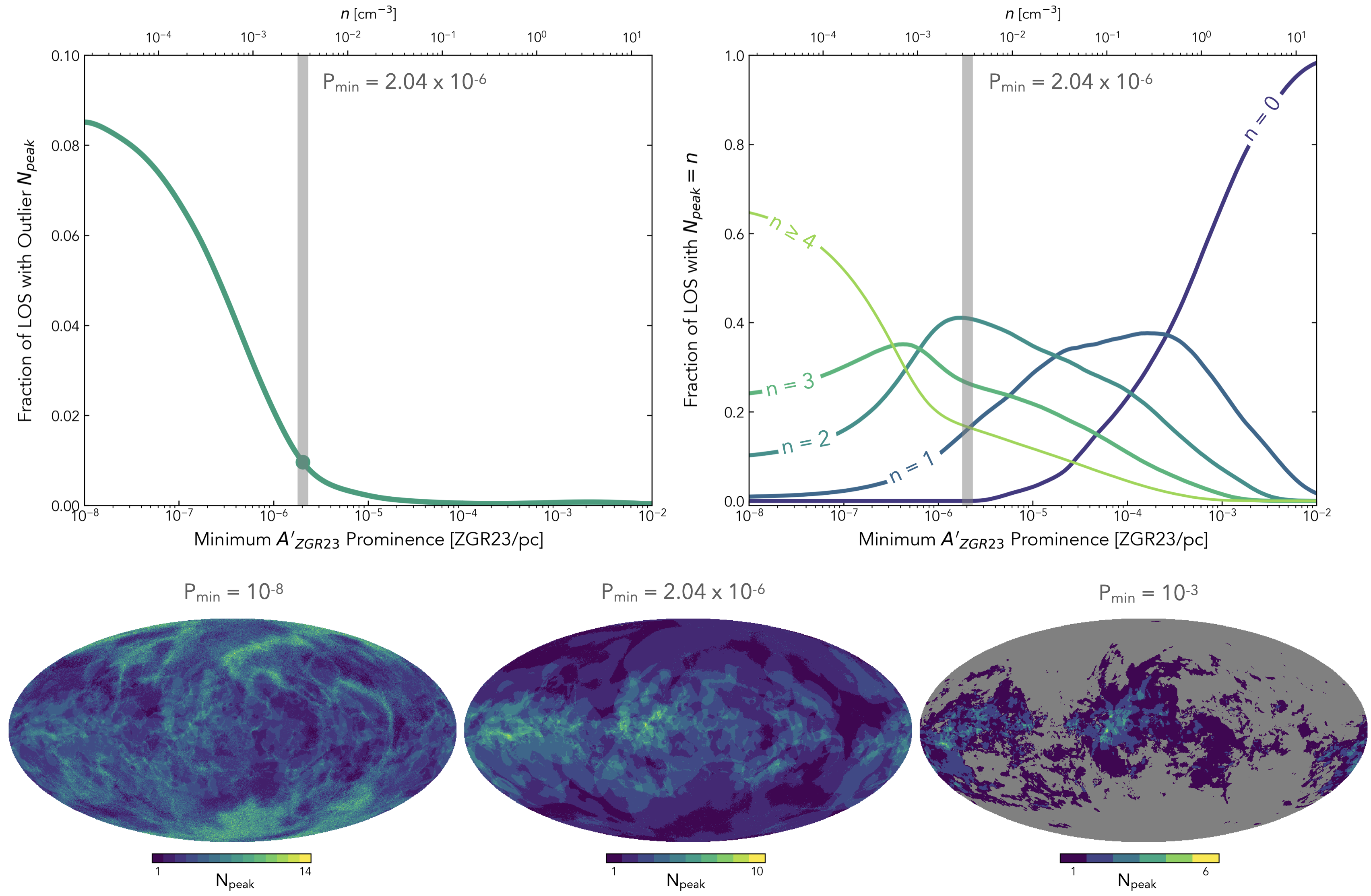
Figure 11: Top left: Fraction of LOS with outlier numbers of peaks, $N_{peak}$, as a function of minimum prominence $P_{\rm{min}}$ required for a local maximum along the LOS to be considered a peak. The selected fiducial $P_{\rm{min}}$ $=2.04\times 10^{-6}$ ZGR23/pc used to generate our model of the Local Bubble is highlighted by the gray line. The secondary x-axis shows the approximate conversion from ZGR23/pc to volume density $n$. Top right: Fraction of LOS with $N_{peak}$ $=n$ as a function of $P_{\rm{min}}$, for $n=0,1,2,3$ and $n\geq 4$. Bottom: Mollweide projections of $N_{peak}$ are shown for $P_{\rm{min}}$ = $10^{-8}$ ZGR23/pc, $2.0\times 10^{-6}$ ZGR23/pc, and $10^{-3}$ ZGR23/pc.

There are two main parameters of interest in our peak finding method: smoothing scale and minimum peak prominence. We select smoothing scale by testing Gaussian smoothing kernel sizes ranging between $\sigma_{smooth}=1$ pc and $\sigma_{smooth}\geq 20$ pc. We find that $\sigma_{smooth}\lesssim 3$ pc is ineffective at smoothing out small stochastic variations in $A^{\prime}_{ZGR23}$, while $\sigma_{smooth}\gtrsim 10$ pc causes narrow but distinct nearby peaks to blend together. We find that $\sigma_{smooth}=7$ pc generally strikes the best balance between smoothing over apparent noise while preserving genuine peaks.

We then estimate what minimum peak prominence is most suited to ignoring noise while preserving detections of high latitude, low-density peaks. We test $P_{\rm{min}}$ ranging from $10^{-8}$ ZGR23/pc to $10^{-2}$ ZGR23/pc (with 100 values of $P_{\rm{min}}$ per dex, evenly spaced in $\log P$), spanning the broad range of differential extinction probed by the E23 map. For each $P_{\rm{min}}$, we performed our peak finding procedure (described in §2.2) and calculated the number of peaks detected along each LOS, $N_{peak}$, within a distance of $d\leq 650$ pc.

We expect that at our well-resolved angular spacing of $N_{\rm{side}}={256}$, adjacent LOS should typically have the same $N_{peak}$, and that LOS with significantly different $N_{peak}$ from their neighboring LOS are likely to have detected some number of small-angular-scale noise-driven peaks. Following this reasoning, we define LOS with “outlier” $N_{peak}$ as LOS where none of their 8 neighboring HEALPix pixels have the same $N_{peak}$.

For each candidate $P_{\rm{min}}$, we perform this outlier calculation and derive the fraction of LOS over the whole sky that have outlier $N_{peak}$. The left panel of Figure 11 shows the fraction of outlier $N_{peak}$ LOS as a function of $P_{\rm{min}}$. We observe a higher fraction (8%) of outlier LOS at very low $P_{\rm{min}}$, which gradually declines as $P_{\rm{min}}$ increases before plateauing to a low fraction ($<0.1\%$) of outlier LOS at very high $P_{\rm{min}}$. The bottom three panels of Figure 11 show $N_{peak}$ over the sky for three representative values of $P_{\rm{min}}$; as $P_{\rm{min}}$ increases, the on-sky distribution of $N_{peak}$ transitions from being noise-dominated, to relatively cohesive across neighboring pixels, to only detecting the highest density dust features.

The “optimal” $P_{\rm{min}}$ for our use case of simultaneously identifying very high density and low density peaks likely falls somewhere in the middle of this range – and, in particular, in the region experiencing the most rapid decline, ranging between $P_{\rm{min}}$ = $10^{-6}$ ZGR23/pc and $P_{\rm{min}}$ = $10^{-5}$ ZGR23/pc. We identify this optimal $P_{\rm{min}}$ as the “knee” of this section of the outlier curve, and approximate the knee’s location as the maximum of the second derivative of the outlier curve (smoothed with a Gaussian kernel of $\sigma=0.1$ dex to reduce the effects of our discrete sampling of $P_{\rm{min}}$). This corresponds to a selected $P_{\rm{min}}$ of $2.04\times 10^{-6}$ ZGR23/pc, a level at which only 0.9% of LOS have outlier $N_{peak}$. The right panel of Figure 11 shows the fraction of LOS with a given $N_{peak}$ $=n$ as a function of $P_{\rm{min}}$ for $n=0,1,2,3$ and $n\geq 4$. At the $P_{\rm{min}}$ we selected, the majority of LOS have two or three peaks.

Appendix B Uncertainty Estimation

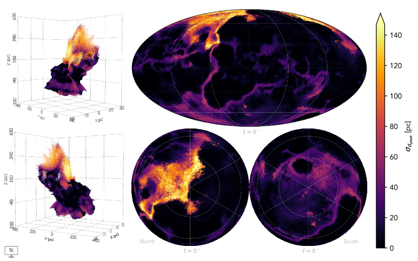
Figure 13: Uncertainty on distance to the Local Bubble’s shell, $\sigma_{d_{peak}}$, derived from the 12 draws of the E23 map, is shown in 3D and in 2D projections. Distance in 3D projection is the mean position in all 12 draws. Interactive 3D figure: https://theo-oneill.github.io/localbubble/sigma_distance/.

To estimate statistical uncertainties on the properties of the Local Bubble’s shell, we apply our peak finding process to each of the 12 draws of the E23 map. The individual draws are generally noisier along the LOS than the posterior mean; we thereform perform our optimal $P_{\rm{min}}$ selection procedure (described in Appendix A) for each draw, and select a $P_{\rm{min}}$ to be used on all 12 draws as the knee of their mean $P_{\rm{min}}$ vs. outlier $N_{peak}$ fraction curve. This yields an optimal $P_{\rm{min}}$ =$1.26\times 10^{-5}$ ZGR23/pc to be used for peak finding in all draws.

We define statistical uncertainties on each derived property of the Local Bubble’s shell as the standard deviation of the equivalent properties in the 12 draws. We expect this procedure should provide a reasonable estimate of statistical uncertainties introduced by the Gaussian Process-based construction of the E23 map; however, it does not account for systematic uncertainties involved in the creation of the map (see E23 for a discussion of these other uncertainties and caveats). Our uncertainty estimates along individual LOS also do not include systematic uncertainties introduced by the assumptions used to convert from measured differential extinction to derived quantities like extinction, volume density, and mass.

As an example of the results of this procedure, Figure 13 shows the uncertainty on distance to the Local Bubble’s shell, $\sigma_{d}$. We find that $\sigma_{d}$ is inversely correlated with dust density, and that $\sigma_{d}$ is typically less than 10 pc in most of the higher density regions. $\sigma_{d}$ is highest in the Northern chimney region, which is unsurprising given how low density the dust is and how wide the shell appears to be in the posterior mean model in this area. This suggests that our estimate of shell thickness in this region is merely an upper limit, and that shell dust is likely contained somewhere within this wide range.

Appendix C Comparison to Pelgrims et al. (2020) Model

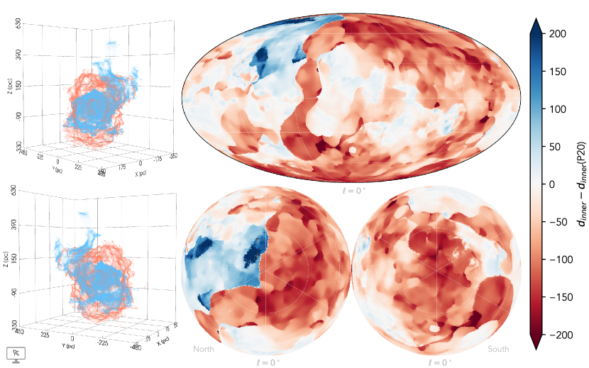
Figure 14: Difference between distance to the Local Bubble’s inner surface in our model vs. the Pelgrims et al. (2020) model is shown in 3D and 2D projections. Interactive 3D figure: https://theo-oneill.github.io/localbubble/compare_pelgrims/

The model of the Local Bubble that has been most widely adopted in recent years was created by Pelgrims et al. (2020, herafter P20) using Lallement et al. (2019, herafter L19)’s 3D dust reddening map generated from Gaia DR2 and 2MASS photometry and astrometry. The L19 map covers a larger volume than the E23 map in the Galactic plane, but smaller towards Galactic north and south (extending from $|x|<3$ kpc, $|y|<3$ kpc, $|z|<400$ pc), and is defined at a lower spatial resolution (a minimum of 25 pc within 1 kpc) than the E23 map.

P20 sampled differential extinction $A^{\prime}_{v}(r)=dA_{v}/dr$ along the LOS at distance intervals of 2.5 pc with an angular spacing of HEALPix $N_{\rm{side}}={128}$ (27’ pixel size), and smoothed each LOS with a Gaussian kernel of $\sigma_{smooth}=25$ pc. They then defined the inner surface of the Local Bubble as the location of the first inflection point in $A^{\prime}_{v}(r)$ ($d^{2}A^{\prime}_{v}(r)/dr^{2}=0$) where the curve transitioned from convex to concave (i.e., from $d^{2}A^{\prime}_{v}(r)/dr^{2}>0$ to $d^{2}A^{\prime}_{v}(r)/dr^{2}<0$). They similarly defined the outer surface as the first inflection point after the inner surface where the curve transitioned from concave to convex.

P20’s model was created to help model the Local Bubble’s magnetic field and infer the orientation of the Galactic magnetic field in the Solar neighborhood, making a smoothed model of the Local Bubble’s surface desirable. To this end, P20 performed iterative spherical harmonic expansions of the inner surface (with a given maximum expansion $l_{\rm{max}}$) to generate smoothed models. Data products released by P20 included the unsmoothed distance to the inner surface as well as smoothed maps of the inner surface at a variety of $l_{\rm{max}}$. Zucker et al. (2022) used the P20 model with $l_{\rm{max}}$ = 10 for their study of Local Bubble-triggered star formation in the Solar Neighborhood.

P20’s inflection point-based procedure was appropriate for defining the inner edge of the Local Bubble in the L19 map due to the relatively large smoothing kernel employed along the LOS ($\sigma_{smooth}=25$ pc, matching the approximate resolution of the L19 map). We find that, for the higher resolution E23 map, we would need to overly smooth our LOS to yield inflection points that span the majority of the observable rise and decline in dust extinction preceding and following a peak. Since many peaks in the E23 map have widths of $<$10 pc and/or fall close to the start of the dust volume probed at $d=69$ pc, employing an overly large level of smoothing causes narrow peaks to blend together and for peaks closer to the Sun to be entirely missed. We therefore prefer to define inner and outer peak edges via a simple prominence-based criterion (described in §2.2), which we find better preserves the morphology of the unsmoothed E23 map.

Figure 14 compares our model of the Local Bubble’s inner surface (degraded to $N_{\rm{side}}={128}$ resolution) to P20’s unsmoothed model in both 2D and 3D. In low latitude regions where dust density is high, the two models are very similar. At higher latitudes, our model generally falls at smaller distances (closer to the Sun) than P20, with the exception of the Northern Chimney feature; P20 finds closed caps to both the North and South, while we find an open Northern cap. We attribute these differences to the difference in the spatial resolution and dust sensitivity of the 3D dust maps used. As future 3D maps of the Solar neighborhood are developed, we expect our understanding of the Local Bubble’s morphology to be further refined.

Appendix D Derivation of Volume Density from Differential Extinction

For a given band $X$ with extinction $A_{X}$, volume density can be derived from differential extinction in the E23 map through the following relationships. Differential extinction at distance slice $i$ can be converted from ZGR23 units to $X$-band as,

$$A^{\prime}_{X,i}=m_{X}A^{\prime}_{ZGR23,i},$$ (D1)

where the coefficient $m_{X}$ comes from ZGR23’s published extinction curve.

Differential extinction is defined per parsec,

$$A^{\prime}_{X,i}=\frac{dA_{X,i}}{1\rm{pc}},$$ (D2)

and can be converted to extinction by multiplying by the radial distance interval $dr_{i}$ between slice $i$ and $i+1$,

$$A_{X,i}=A^{\prime}_{X,i}dr_{i}=\frac{dA_{X,i}}{1\rm{pc}}dr_{i}.$$ (D3)

By assuming the ratio of hydrogen column density to $X$-band extinction is constant,

$$A_{X}/N_{H}\simeq\alpha\ \rm{mag}\ \rm{cm}^{2},$$ (D4)

volume density can be derived as

$$n_{i}=\frac{\#}{dv_{i}}=\frac{N_{H}da_{i}}{dv_{i}}=\frac{A_{X,i}}{\alpha}\frac{da_{i}}{dv_{i}},$$ (D5)

where $da_{i}$ is the physical area of the slice at distance $d_{i}$, and $dv_{i}$ is the volume between slice $i$ and $i+1$.

This leads to a relationship between ZGR23 differential extinction and volume density of,

$$n_{i}=\frac{m_{X}}{(A_{X}/N_{H})}\frac{dA_{ZGR23,i}}{1\rm{pc}}\frac{dr_{i}da_{i}}{dv_{i}}.$$ (D6)

Since $dv_{i}=da_{i}dr_{i}$, this simplifies to

$$n_{i}=\frac{m_{X}}{(A_{X}/N_{H})}\frac{A^{\prime}_{ZGR23,i}}{(3.086\times 10^{18})}$$ (D7)

for $n_{i}$ in units of cm^-3, where the factor $3.086\times 10^{18}$ is introduced to convert between parsecs and centimeters.

References

- Albert & Danly (2004) Albert, C. E., & Danly, L. 2004, in ASSL, Vol. 312, High Velocity Clouds, ed. H. van Woerden, B. P. Wakker, U. J. Schwarz, & K. S. de Boer, 73
- Alves et al. (2020) Alves, J., Zucker, C., Goodman, A. A., et al. 2020, Nature, 578, 237
- Anderson et al. (2019) Anderson, L. D., Wenger, T. V., Armentrout, W. P., Balser, D. S., & Bania, T. M. 2019, ApJ, 871, 145
- Astropy Collaboration et al. (2013) Astropy Collaboration, Robitaille, T. P., Tollerud, E. J., et al. 2013, A&A, 558, A33
- Astropy Collaboration et al. (2018) Astropy Collaboration, Price-Whelan, A. M., Sipőcz, B. M., et al. 2018, AJ, 156, 123
- Astropy Collaboration et al. (2022) Astropy Collaboration, Price-Whelan, A. M., Lim, P. L., et al. 2022, ApJ, 935, 167
- Bacchini et al. (2019) Bacchini, C., Fraternali, F., Iorio, G., & Pezzulli, G. 2019, A&A, 622, A64
- Baumgartner & Breitschwerdt (2013) Baumgartner, V., & Breitschwerdt, D. 2013, A&A, 557, A140
- Beaumont et al. (2015) Beaumont, C., Goodman, A., & Greenfield, P. 2015, in ASPC, Vol. 495, ADASS XXIV, ed. A. R. Taylor & E. Rosolowsky, 101
- Benítez et al. (2002) Benítez, N., Maíz-Apellániz, J., & Canelles, M. 2002, Phys. Rev. Lett., 88, 081101
- Bialy et al. (2021) Bialy, S., Zucker, C., Goodman, A., et al. 2021, ApJ, 919, L5
- Bracco et al. (2020) Bracco, A., Bresnahan, D., Palmeirim, P., et al. 2020, A&A, 644, A5
- Brandt et al. (1971) Brandt, J. C., Stecher, T. P., Crawford, D. L., & Maran, S. P. 1971, ApJ, 163, L99
- Bregman (1980) Bregman, J. N. 1980, ApJ, 236, 577
- Breitschwerdt et al. (2016) Breitschwerdt, D., Feige, J., Schulreich, M. M., et al. 2016, Nature, 532, 73
- Cardelli et al. (1989) Cardelli, J. A., Clayton, G. C., & Mathis, J. S. 1989, ApJ, 345, 245
- Cox & Reynolds (1987) Cox, D. P., & Reynolds, R. J. 1987, ARA&A, 25, 303
- Cox & Smith (1974) Cox, D. P., & Smith, B. W. 1974, ApJ, 189, L105
- Dawson (2013) Dawson, J. R. 2013, PASA, 30, e025
- de Avillez & Berry (2001) de Avillez, M. A., & Berry, D. L. 2001, MNRAS, 328, 708
- de Avillez & Breitschwerdt (2005) de Avillez, M. A., & Breitschwerdt, D. 2005, A&A, 436, 585
- Dickey & Lockman (1990) Dickey, J. M., & Lockman, F. J. 1990, ARA&A, 28, 215
- Draine (2003) Draine, B. T. 2003, ARA&A, 41, 241
- Draine (2009) Draine, B. T. 2009, in ASPC, Vol. 414, Cosmic Dust - Near and Far, ed. T. Henning, E. Grün, & J. Steinacker, 453
- Edenhofer et al. (2022) Edenhofer, G., Leike, R. H., Frank, P., & Enßlin, T. A. 2022, arXiv e-prints, arXiv:2206.10634
- Edenhofer et al. (2023) Edenhofer, G., Zucker, C., Frank, P., et al. 2023, arXiv e-prints, arXiv:2308.01295
- Edenhofer et al. (2024) Edenhofer, G., Frank, P., Roth, J., et al. 2024, arXiv e-prints, arXiv:2402.16683
- Farhang et al. (2019) Farhang, A., van Loon, J. T., Khosroshahi, H. G., Javadi, A., & Bailey, M. 2019, NatAs, 3, 922
- Ferriere et al. (1991) Ferriere, K. M., Mac Low, M.-M., & Zweibel, E. G. 1991, ApJ, 375, 239
- Fesen et al. (2021) Fesen, R. A., Drechsler, M., Weil, K. E., et al. 2021, ApJ, 920, 90
- Fielding et al. (2018) Fielding, D., Quataert, E., & Martizzi, D. 2018, MNRAS, 481, 3325
- Fielding et al. (2017) Fielding, D., Quataert, E., Martizzi, D., & Faucher-Giguère, C.-A. 2017, MNRAS, 470, L39
- Frisch (1986) Frisch, P. C. 1986, AdSpR, 6, 345
- Frisch & York (1983) Frisch, P. C., & York, D. G. 1983, ApJ, 271, L59
- Fuchs et al. (2006) Fuchs, B., Breitschwerdt, D., de Avillez, M. A., Dettbarn, C., & Flynn, C. 2006, MNRAS, 373, 993
- Gensior et al. (2023) Gensior, J., Feldmann, R., Mayer, L., et al. 2023, MNRAS, 518, L63
- Girichidis et al. (2016) Girichidis, P., Walch, S., Naab, T., et al. 2016, MNRAS, 456, 3432
- Górski et al. (2005) Górski, K. M., Hivon, E., Banday, A. J., et al. 2005, ApJ, 622, 759
- Green (2018) Green, G. M. 2018, JOSS, 3, 695
- Green et al. (2015) Green, G. M., Schlafly, E. F., Finkbeiner, D. P., et al. 2015, ApJ, 810, 25
- Grenier et al. (1989) Grenier, I. A., Lebrun, F., Arnaud, M., Dame, T. M., & Thaddeus, P. 1989, ApJ, 347, 231
- Gum (1952) Gum, C. S. 1952, Obs, 72, 151
- Harris et al. (2020) Harris, C. R., Millman, K. J., van der Walt, S. J., et al. 2020, Nature, 585, 357
- Heiles (1998) Heiles, C. 1998, ApJ, 498, 689
- HI4PI Collaboration et al. (2016) HI4PI Collaboration, Ben Bekhti, N., Flöer, L., et al. 2016, A&A, 594, A116
- Hunter (2007) Hunter, J. D. 2007, CSE, 9, 90
- Inutsuka et al. (2015) Inutsuka, S.-i., Inoue, T., Iwasaki, K., & Hosokawa, T. 2015, A&A, 580, A49
- Jordi et al. (2010) Jordi, C., Gebran, M., Carrasco, J. M., et al. 2010, A&A, 523, A48
- Joubaud et al. (2019) Joubaud, T., Grenier, I. A., Ballet, J., & Soler, J. D. 2019, A&A, 631, A52
- Jurić et al. (2008) Jurić, M., Ivezić, Ž., Brooks, A., et al. 2008, ApJ, 673, 864
- Kim & Ostriker (2018) Kim, C.-G., & Ostriker, E. C. 2018, ApJ, 853, 173
- Kim et al. (2017) Kim, C.-G., Ostriker, E. C., & Raileanu, R. 2017, ApJ, 834, 25
- Knies et al. (2018) Knies, J. R., Sasaki, M., & Plucinsky, P. P. 2018, MNRAS, 477, 4414
- Konietzka et al. (2024) Konietzka, R., Goodman, A. A., Zucker, C., et al. 2024, arXiv e-prints, arXiv:2402.12596
- Koo & McKee (1992) Koo, B.-C., & McKee, C. F. 1992, ApJ, 388, 93
- Korpi et al. (1999) Korpi, M. J., Brandenburg, A., Shukurov, A., & Tuominen, I. 1999, A&A, 350, 230
- Kuntz & Danly (1996) Kuntz, K. D., & Danly, L. 1996, ApJ, 457, 703
- Lallement et al. (2019) Lallement, R., Babusiaux, C., Vergely, J. L., et al. 2019, A&A, 625, A135
- Lallement et al. (2014) Lallement, R., Vergely, J. L., Valette, B., et al. 2014, A&A, 561, A91
- Lallement et al. (2003) Lallement, R., Welsh, B. Y., Vergely, J. L., Crifo, F., & Sfeir, D. 2003, A&A, 411, 447
- Leike & Enßlin (2019) Leike, R. H., & Enßlin, T. A. 2019, A&A, 631, A32
- Leike et al. (2020) Leike, R. H., Glatzle, M., & Enßlin, T. A. 2020, A&A, 639, A138
- Linsky & Redfield (2021) Linsky, J. L., & Redfield, S. 2021, ApJ, 920, 75
- Liu et al. (2017) Liu, W., Chiao, M., Collier, M. R., et al. 2017, ApJ, 834, 33
- Lockman et al. (1986) Lockman, F. J., Jahoda, K., & McCammon, D. 1986, ApJ, 302, 432
- Mac Low & McCray (1988) Mac Low, M.-M., & McCray, R. 1988, ApJ, 324, 776
- Mac Low et al. (1989) Mac Low, M.-M., McCray, R., & Norman, M. L. 1989, ApJ, 337, 141
- Maíz-Apellániz (2001a) Maíz-Apellániz, J. 2001a, ApJ, 560, L83
- Maíz-Apellániz (2001b) —. 2001b, AJ, 121, 2737
- Marchal & Martin (2023) Marchal, A., & Martin, P. G. 2023, ApJ, 942, 70
- Markkanen (1979) Markkanen, T. 1979, A&A, 74, 201
- McCullough et al. (2002) McCullough, P. R., Fields, B. D., & Pavlidou, V. 2002, ApJ, 576, L41
- McKee & Ostriker (1977) McKee, C. F., & Ostriker, J. P. 1977, ApJ, 218, 148
- McKinney (2010) McKinney, W. 2010, in Proc. 9th Python in Science Conf., ed. Stéfan van der Walt & Jarrod Millman, 56
- Norman & Ikeuchi (1989) Norman, C. A., & Ikeuchi, S. 1989, ApJ, 345, 372
- Ocker et al. (2024) Ocker, S. K., Cordes, J. M., Chatterjee, S., et al. 2024, MNRAS, 527, 7568
- Olano et al. (2006) Olano, C. A., Meschin, P. I., & Niemela, V. S. 2006, MNRAS, 369, 867
- Orr et al. (2022a) Orr, M. E., Fielding, D. B., Hayward, C. C., & Burkhart, B. 2022a, ApJ, 924, L28
- Orr et al. (2022b) —. 2022b, ApJ, 932, 88
- Panopoulou & Lenz (2020) Panopoulou, G. V., & Lenz, D. 2020, ApJ, 902, 120
- Patra (2020) Patra, N. N. 2020, MNRAS, 499, 2063
- Pelgrims et al. (2020) Pelgrims, V., Ferrière, K., Boulanger, F., Lallement, R., & Montier, L. 2020, A&A, 636, A17
- Plucinsky et al. (1996) Plucinsky, P. P., Snowden, S. L., Aschenbach, B., et al. 1996, ApJ, 463, 224
- Pon et al. (2016) Pon, A., Ochsendorf, B. B., Alves, J., et al. 2016, ApJ, 827, 42
- Puspitarini & Lallement (2012) Puspitarini, L., & Lallement, R. 2012, A&A, 545, A21
- Reynolds & Ogden (1979) Reynolds, R. J., & Ogden, P. M. 1979, ApJ, 229, 942
- Robitaille et al. (2019) Robitaille, T., Beaumont, C., Qian, P., Borkin, M., & Goodman, A. 2019, glueviz v0.15.2: multidimensional data exploration
- Röhser et al. (2016) Röhser, T., Kerp, J., Lenz, D., & Winkel, B. 2016, A&A, 596, A94
- Seabold & Perktold (2010) Seabold, S., & Perktold, J. 2010, in Proc. 9th Python in Science Conf., ed. Stéfan van der Walt & Jarrod Millman, 92
- Sfeir et al. (1999) Sfeir, D. M., Lallement, R., Crifo, F., & Welsh, B. Y. 1999, A&A, 346, 785
- Shapiro & Field (1976) Shapiro, P. R., & Field, G. B. 1976, ApJ, 205, 762
- Snowden et al. (1998) Snowden, S. L., Egger, R., Finkbeiner, D. P., Freyberg, M. J., & Plucinsky, P. P. 1998, ApJ, 493, 715
- Snowden et al. (2015) Snowden, S. L., Koutroumpa, D., Kuntz, K. D., Lallement, R., & Puspitarini, L. 2015, ApJ, 806, 120
- Soler et al. (2018) Soler, J. D., Bracco, A., & Pon, A. 2018, A&A, 609, L3
- Soler et al. (2023) Soler, J. D., Zucker, C., Peek, J. E. G., et al. 2023, A&A, 675, A206
- Sullivan & Kaszynski (2019) Sullivan, C. B., & Kaszynski, A. 2019, JOSS, 4, 1450
- Sushch et al. (2011) Sushch, I., Hnatyk, B., & Neronov, A. 2011, A&A, 525, A154
- Swiggum et al. (2022) Swiggum, C., Alves, J., D’Onghia, E., et al. 2022, A&A, 664, L13
- Tomisaka (1998) Tomisaka, K. 1998, MNRAS, 298, 797
- Trzesiok et al. (2021) Trzesiok, A., tgandor, Kostur, M., et al. 2021, K3D-tools/K3D-jupyter: 2.11.0
- van der Velden (2020) van der Velden, E. 2020, JOSS, 5, 2004
- Vergely et al. (2001) Vergely, J. L., Freire Ferrero, R., Siebert, A., & Valette, B. 2001, A&A, 366, 1016
- Wakker (2004) Wakker, B. P. 2004, in ASSL, Vol. 312, High Velocity Clouds, ed. H. van Woerden, B. P. Wakker, U. J. Schwarz, & K. S. de Boer, 25
- Walch et al. (2015) Walch, S., Girichidis, P., Naab, T., et al. 2015, MNRAS, 454, 238
- Welsh (1991) Welsh, B. Y. 1991, ApJ, 373, 556
- Welsh et al. (2004) Welsh, B. Y., Sallmen, S., & Lallement, R. 2004, A&A, 414, 261
- Welsh et al. (1999) Welsh, B. Y., Sfeir, D. M., Sirk, M. M., & Lallement, R. 1999, A&A, 352, 308
- Welsh & Shelton (2009) Welsh, B. Y., & Shelton, R. L. 2009, Ap&SS, 323, 1
- Whitworth et al. (1994) Whitworth, A. P., Bhattal, A. S., Chapman, S. J., Disney, M. J., & Turner, J. A. 1994, AA, 290, 421
- Zhang et al. (2023) Zhang, X., Green, G. M., & Rix, H.-W. 2023, MNRAS, 524, 1855
- Zonca et al. (2019) Zonca, A., Singer, L., Lenz, D., et al. 2019, JOSS, 4, 1298
- Zucker et al. (2021) Zucker, C., Goodman, A., Alves, J., et al. 2021, ApJ, 919, 35
- Zucker et al. (2022) Zucker, C., Goodman, A. A., Alves, J., et al. 2022, Nature, 601, 334