Bayesian Inference for High-dimensional Time Series by Latent Process Modeling

Abstract

Time series data arising in many applications nowadays are high-dimensional. A large number of parameters describe features of these time series. Sensible inferences on these parameters with limited data are possible if some underlying lower-dimensional structure is present. We propose a novel approach to modeling a high-dimensional time series through several independent univariate time series, which are then orthogonally rotated and sparsely linearly transformed. With this approach, any specified intrinsic relations among component time series given by a graphical structure can be maintained at all time snapshots. We call the resulting process an Orthogonally-rotated Univariate Time series (OUT). Key structural properties of time series such as stationarity and causality can be easily accommodated in the OUT model. For Bayesian inference, we put suitable prior distributions on the spectral densities of the independent latent times series, the orthogonal rotation matrix, and the common precision matrix of the component times series at every time point. A likelihood is constructed using the Whittle approximation for univariate latent time series. An efficient Markov Chain Monte Carlo (MCMC) algorithm is developed for posterior computation. We study the convergence of the pseudo-posterior distribution based on the Whittle likelihood for the model’s parameters upon developing a new general posterior convergence theorem for pseudo-posteriors. We find that the posterior contraction rate for independent observations essentially prevails in the OUT model under very mild conditions on the temporal dependence described in terms of the smoothness of the corresponding spectral densities. Through a simulation study, we compare the accuracy of estimating the parameters and identifying the graphical structure with other approaches. We apply the proposed methodology to analyze a dataset on different industrial components of the US gross domestic product between 2010 and 2019 and predict future observations.

Keywords: Bayesian, Cholesky, High dimensional, Pseudo-posterior, Time series, Whittle

1 Introduction

Understanding the intrinsic dependence structure among a set of random variables, assessed by the conditional dependence between two variables given the remaining variables, is a fundamental problem in statistics. Pairs of variables that are intrinsically dependent are connected by an edge, thus giving a graphical representation of the interrelations. Among probabilistic models for a relational graph, Gaussian Graphical Models (GGM) have the appealing property that conditional independence of a pair of variables given the others is equivalent to the zero-value of the corresponding off-diagonal entry of the precision matrix. A rich literature on estimating the graphical structure can be found in classical books like Lauritzen (1996); Koller and Friedman (2009); see also Maathuis et al. (2019) and references therein for more recent results. The papers Jordan and Sejnowski (2001); Meinshausen and Bühlmann (2006); Yuan and Lin (2007); Friedman et al. (2008); Bühlmann and van de Geer (2011); Wang (2012); Wang and Li (2012); Banerjee and Ghosal (2014) provided some early developments of statistical estimation and structure learning methods in a GGM under both frequentist and Bayesian frameworks. Some of the follow-up developments have been on nonparanormal graphical model Liu et al. (2012); Mulgrave and Ghosal (2020), pseudo-likelihood based CONCORD (Khare et al., 2015), CLIME (Cai et al., 2011), Gaussian copula graphical model (Dobra et al., 2011; Liu et al., 2012), other Markov random field based models (Wainwright et al., 2006; Yang et al., 2013; Chen et al., 2014; Roy and Dunson, 2020) etc. Since their introduction, GGM and closely related models have been applied to many disciplines including neuroimaging applications, application to genetics, financial applications, political and socioeconomic applications, and network analysis. A typical modern application requires learning graphical structures in a high-dimensional setting. Most work on the inference for graphical models has been restricted to independently and identically distributed multivariate observations. In this paper, we use the contemporaneous precision matrix of a stationary time series to estimate the graph along the line of Qiu et al. (2016); Zhang and Wu (2017). It turns out though that under the proposed model, the graphical structure encoded by the contemporaneous precision matrix encodes that of a stationary multivariate time series in the stronger sense as described in Dahlhaus (2000). The multivariate data considered in this article are regularly spaced vector time series. However, we do not make modeling assumptions on the temporal dynamics using any common parametric vector time series models, treating the autocorrelation structure as a nuisance parameter in the graph learning problem. We propose a semi-parametric model called Orthogonally-rotated Univariate Time series (OUT) for the vector time series data. This model parameterizes parameters in the graphical structure explicitly while the temporal structure is modeled nonparametrically. A Bayesian graph learning framework is used that provides efficient estimation and automatic uncertainty quantification through the resulting posterior distribution.

Several different graphical structures could be of interest in a vector time series model. A ‘contemporaneous stationary graphical’ structure is where the graphical structure is encoded in the marginal precision matrix of a stationary Gaussian time series. In a contemporaneous stationary graph, the nodes are the coordinate variables of the vector time series. In stationary time series, one may also construct a graph with the nodes representing the entire coordinate processes. This would be a ‘stationary graphical’ structure. Conditional independence in such a graph can be expressed equivalently in terms of the absence of partial spectral coherence between two nodal series; see Dahlhaus (2000). High dimensional series estimation of such stationary graphs have been investigated by Jung et al. (2015); Fiecas et al. (2019). Recently, Basu and Rao (2023) has extended the stationary graphical models to non-stationary time series. Some authors have studied time series for graphs and networks; see, for instance, Basu et al. (2015); Ma and Michailidis (2016).

A popular class of multivariate time series model that looks at lower dimensional structures is the high-dimensional Dynamic Factor Model (DFM). The DFM finds use in many economic applications as well as in other areas. Since its initial introduction to the econometric literature, a large body of work has emerged; see Forni et al. (2000); Forni and Lippi (2001); Bai and Ng (2002); Bai (2003); Deistler et al. (2010); Stock and Watson (2012); Bottegal and Picci (2015); Barigozzi et al. (2023) and also Lippi et al. (2023) for a recent survey of related works. While the DFM is particularly suited for estimating latent lower-dimensional processes driving the dynamics, the parameterization is not suitable for the estimation of the graphical structure. The proposed semiparametric model in this paper closely resembles DFM. However, unlike the traditional DFM, the proposed model allows a full-dimensional latent process without an idiosyncratic term. Reduction in complexity comes from the assumption of independence of the latent processes. The direct parameterization of the contemporaneous precision matrix provides a certain advantage over traditional DFM when it comes to graph estimation. The proposed model and dynamic factor models both have symmetric autocovariance functions. However, the interpretation of the marginal precision matrix of $\bm{Y}_{t}$ is the main focus of this work whereas the traditional factor modeling framework is not amenable to such analysis. The full-dimensional independent latent dynamic processes are analogous to the framework of Independent Component Analysis, but the objectives are different. In the proposed framework, the latent sources are all Gaussian and hence cannot be separated without additional constraints, but the primary objective of learning the graphical structure can be done consistently.

This article proposes a latent time series model based on a hidden lower-dimensional structure in the high-dimensional time series. Specifically, let $\bm{Y}_{t}$ be a $p$-dimensional centered Gaussian time series observed at $T$ times points $\{1,\ldots,T\}$, modeled as $\bm{Y}_{t}=\bm{A}\bm{Z}_{t}$, where $\bm{Z}_{t}$ is a $p$-variate centered Gaussian time series consisting of independent components unit variance at every $t$. Then the dispersion matrix of $\bm{Y}_{t}$ is $\bm{\Sigma}=\bm{A}\bm{A}^{\rm T}$. The precision matrix $\bm{\Omega}=\bm{\Sigma}^{-1}$ of $\bm{Y}_{t}$ determines the conditional independence structure in the time series at a given time point in that the $(j,k)$th off-diagonal entry of $\bm{\Omega}$ is $0$ if and only if $Y_{t,j}$ and $Y_{t,k}$ are independent given $\{Y_{l,t}:l=1,\ldots,p,\,l\neq j,k\}$. The necessity of the condition holds for non-Gaussian time series as well. However, for non-Gaussian variables, the graph reduces to a partial correlation graph instead of a conditional independence graph. We let $\bm{\Sigma}^{1/2}$ denote the positive definite Cholesky square root of $\bm{\Sigma}$, and write $\bm{A}$ as $\bm{\Sigma}^{1/2}\bm{U}$, where $\bm{U}$ is a $p\times p$ orthogonal matrix, leading to the representation $\bm{Y}_{t}=\bm{\Sigma}^{1/2}\bm{U}\bm{Z}_{t}$ in terms of the uniquely identifiable parameter $\bm{\Sigma}^{1/2}$ or the associated precision matrix $\bm{\Omega}$. Since the model is represented by orthogonally rotating an ensemble of $p$ independent univariate time series, we shall call it the Orthogonally-rotated Univariate Time series (OUT) model. In the OUT model, the graphical dependence structure as encoded by the elements of the precision matrix remains invariant over time, which will be our primary learning target. Assuming a sparse structure of $\bm{\Omega}$, the graph may be identified by estimating $\bm{\Omega}$. We use a Bayesian approach and induce a graphical structure by putting a prior on sparse precision matrices through a modified Cholesky decomposition and a sparse prior on the components of the Cholesky factor.

Existing methods for high-dimensional time series that estimate the graphical dependence through a sparse precision matrix, such as Kolar et al. (2010); Chen et al. (2013) may not maintain properties such as stationarity, and causality in the estimated processes. The proposed OUT model provides a natural avenue for modeling stationary, causal, high-dimensional time series with interpretable graphical dependence structure among components. This graph learning in high-dimensional causal stationary processes with $p$ dimensional latent structure is possible because of the assumed independence of the latent time series and facilitates separation of the individual latent series in the estimation process. The spectral densities of the univariate time series are modeled using B-splines, with an additional assumption of low-rankness on the coefficients. Because of the underlying independence structure, the Whittle approximate likelihood can be conveniently used for inference in the OUT model. This allows a simpler expansion of the pseudo-likelihood for studying posterior convergence properties.

One of the main contributions of the paper is a general posterior convergence theorem for models such as our multivariate time series analysis where the convenience of showing convergence under the simpler pseudo-likelihood can be transported to that under the true likelihood using a change of measure argument. We establish that the posterior contraction rate for the precision matrix in terms of the Frobenius norm is given by $\sqrt{((p+s)\log p)/T}$ provided the spectral densities of the latent independent univariate time series are sufficiently smooth, where $s$ stands for the number of non-zero off-diagonal entries of the true precision matrix. The rate thus coincides with the optimal rate for the estimation of a sparse precision matrix with respect to the Frobenius norm for independent observations attained by the graphical lasso for independent data (cf. Rothman et al. (2008)) and also by an analogous Bayesian method developed by Banerjee and Ghosal (2015). Thus in the dependence setup of an OUT model, a precision matrix can be learned with the same level of accuracy as with independent observations under sparsity.

The paper is organized as follows. In Section 2, we formally introduce the OUT model and discuss its properties and convenient parameterization. The pseudo-likelihood based on the Whittle approximation, specification of prior distributions, and posterior sampling strategies are described in Section 3. Convergence properties of the posterior distribution are studied in Section 4. Extensive simulation studies to compare the performance of the proposed Bayesian method based on OUT modeling with other possible methods are carried out in Section 5. A dataset on different industrial components of the US gross domestic product between 2010 and 2019 is analyzed in Section 6.

2 Model and parameterization

2.1 Notations and preliminaries

We first describe the notations we follow in this article. Vectors are column-vectors by default and will be denoted by boldface lower-case English or Greek letters or upper-case English letters, while matrices will be denoted by boldface uppercase English or Greek letters. To denote a component of a vector or an entry of a matrix, we shall use the non-bold form of the letter along with the corresponding subscript(s). The transpose of a matrix $\bm{A}$ is denoted by $\bm{A}^{\rm T}$, and for a square matrix, $\mathrm{tr}(\bm{A})$, $\det(\bm{A})$ and $\bm{A}^{-1}$ respectively denote the trace, the determinant, and the inverse (if exists) of $\bm{A}$. The vectorization $\mathrm{vec}(\bm{A})$ of a matrix $\bm{A}$ stacks the columns of $\bm{A}$ in a single column, while the half-vectorization $\mathrm{vech}(\bm{A})$ of a symmetric matrix is the same operation without repeating the identical entries originating from symmetry. We recall the following useful result.

For a nonnegative definite matrix $\bm{A}$, a square root $\bm{B}$ is any matrix such that $\bm{B}\bm{B}^{\rm T}=\bm{A}$, while the unique nonnegative definite square root is denoted by $\bm{A}^{1/2}$. The symbol $\bm{0}$ will stand for a zero-vector or a zero-matrix depending on the context, $\bm{1}$ a vector of ones, and $\bm{I}_{p}$ will denote the $p\times p$-identity matrix. A diagonal matrix $\bm{A}$ whose diagonal entries form a vector $\bm{a}$ will be denoted by $\mathrm{Diag}(\bm{a})$, and conversely, we write $\bm{a}=\mathrm{diag}(\bm{A})$. The same convention will be also used for block-diagonal matrices. The Kronecker product of two matrices will be denoted by $\otimes$ and the Hadamard product, standing for entrywise multiplication when the two matrices have identical dimensions, will be denoted by $\odot$. We shall use $\|\cdot\|_{2}$ to denote the Euclidean norm of a vector, $\|\cdot\|_{\infty}$ the maximum absolute value of the entries, and $\|\bm{x}\|_{0}$ for the number of non-zero entries of $\bm{x}$. For a matrix $\bm{A}$, the Frobenius norm $\|\bm{A}\|_{\mathrm{F}}=\|\mathrm{vec}(\bm{A})\|_{2}$ is the Euclidean norm of its vectorization, the operator norm is given by $\|\bm{A}\|_{\mathrm{op}}=\sup\{\|\bm{A}\bm{x}\|_{2}:\|\bm{x}\|_{2}\leq 1\}$ and the $\ell_{0}$-norm by $\|\bm{A}\|_{0}=\|\mathrm{vec}(\bm{A})\|_{0}$. Let $\Phi$ and $\phi$ stand for the cumulative distribution function and the probability density function of standard normal, respectively. The notation $\mathrm{N}_{p}(\bm{\mu},\bm{\Sigma})$ stands for the $p$-variate normal measure with mean $\bm{\mu}$ and dispersion matrix $\bm{\Sigma}$, and its density will be denoted by $\phi_{p}(\cdot;\bm{\mu},\bm{\Sigma})$. We shall use the notations $\mathbbm{1}$ for the indicator function and $\delta_{0}$ for the degenerate probability measure at $0$. Let $\mathrm{E}$ stand for the expectation operator and $\mathrm{D}$ for the dispersion matrix operator of a random vector. The symbols $\lesssim$, $\ll$, and $\asymp$ will respectively stand for domination by a constant multiple, strict domination in the order of growth or decay, and equality of the order of growth or decay for two given sequences of numbers.

We also recall some useful relations between matrix norms. For a square matrix $\bm{A}$, $\|\bm{A}\|_{\mathrm{F}}^{2}=\mathrm{tr}(\bm{A}\bm{A}^{\rm T})$, $\|\bm{A}\|_{\mathrm{op}}\leq\|\bm{A}\|_{\mathrm{F}}$, and for two square matrices $\bm{A}$ and $\bm{B}$, $\|\bm{A}\bm{B}\|_{\mathrm{F}}\leq\min\{\|\bm{A}\|_{\mathrm{F}}\|\bm{B}\|_{\mathrm{op}},\|\bm{A}\|_{\mathrm{op}}\|\bm{B}\|_{\mathrm{F}}\}$.

2.2 The OUT model

We begin with the formal introduction of an OUT model.

Definition 1 (OUT Process).

A $p$-dimensional centered time series $\bm{Y}_{t}$, $t=1,\ldots,T$, is an Orthogonally-rotated Univariate Time series (OUT) with marginal positive definite covariance matrix $\bm{\Sigma}$ if it admits a representation

$$\bm{Y}_{t}=\bm{\Sigma}^{1/2}\bm{U}\bm{Z}_{t},$$ (2.1)

where $\bm{\Sigma}^{1/2}$ is the lower triangular square root of $\bm{\Sigma}$, $\bm{U}$ is a $p\times p$ orthogonal matrix with determinant $+1$ and $\bm{Z}_{t}=(Z_{1,t},Z_{2,t},\ldots,Z_{p,t})^{\rm T}$ is a vector of independent centered time-series with unit variances.

Since the distribution of any component of the process $(\bm{Z}_{t}:t=1,\ldots,T)$ remains invariant under a sign change, we can assume without loss of generality that $\bm{U}$ has determinant $+1$, by switching the sign of a component of $(\bm{Z}_{t}:t=1,\ldots,T)$, if necessary. Thus we can consider $\bm{U}$ to be a special orthogonal matrix.

Recall that the autocovariance function of a centered multivariate time series $(\bm{X}_{t}:t=0,1,\ldots)$ is defined by $\mbox{\boldmath$\Gamma$}(h,t;\bm{X})=\mathrm{E}[\bm{X}_{t}\bm{X}_{t+h}^{\rm T}]$. A multivariate time series $(\bm{X}_{t}:t=0,1,\ldots)$ is called (strictly) stationary if for any time shift $h$, $(\bm{X}_{t+h}:t=0,1,\ldots)$ has the same joint distribution as $(\bm{X}_{t}:t=0,1,\ldots)$. In that case, the autocovariance function (ACVF) is free of $t$ and depends only on $h$. For a centered Gaussian time series, the converse also holds. A process is called covariance stationary if the ACVF is free of $t$. For a covariance-stationary univariate time series $(X_{t}:t=0,1,\ldots)$ with short-memory, that is, if the autocovariance function $(\gamma(h):h=0,1,\ldots)$ is summable, the spectral density is defined to be $f(\omega)=(2\pi)^{-1}\sum_{h=0}^{\infty}\gamma(h)e^{-ih\omega}$, $\omega\in[-\pi,\pi]$. For a short-memory covariance-stationary multivariate time series $(\bm{X}_{t}:t=0,1,\ldots)$, the spectral density matrix $\bm{F}(\omega;\bm{X})$ is defined to be $(2\pi)^{-1}\sum_{h=0}^{\infty}\mbox{\boldmath$\Gamma$}(h,t;\bm{X})e^{-ih\omega}$, $\omega\in[-\pi,\pi]$. Finally, a time series $(\bm{X}_{t}:t=0,1,\ldots)$ is called causal if for all $t$, $\bm{X}_{t}$ can be expressed as $\bm{H}_{t}(\bm{e}_{t},\bm{e}_{t-1},\ldots)$ for some process $(\bm{e}_{t}:t=0,\pm 1,\pm 2,\ldots)$, where $\bm{H}_{t}$ is a vector-valued function possibly dependent on $t$.

Proposition 1 (Properties of OUT).

The OUT process has the following properties.

• The dispersion matrix of $\bm{Y}_{t}$ is given by $\mathrm{D}(\bm{Y}_{t})=\bm{\Sigma}$ and the precision matrix $\bm{\Omega}=\bm{\Sigma}^{-1}$ for every $t$.

• The ACVF of $(\bm{Y}_{t}:t=0,1,\ldots)$ is $\mbox{\boldmath$\Gamma$}(h,t;\bm{Y})\bm{\Sigma}^{-1/2}\mbox{\boldmath$\Gamma$}(h,t;\bm{Z})(\bm{\Sigma}^{-1/2})^{\rm T}$, where $\mbox{\boldmath$\Gamma$}(\cdot,t;\bm{Z})$ is the ACVF of $(\bm{Z}_{t}:t=0,1,\ldots)$, for all time epoch $t$. The function is symmetric in the lag-variable, i.e. $\mbox{\boldmath$\Gamma$}(-h,t;\bm{Y})=\mbox{\boldmath$\Gamma$}(h,t;\bm{Y})$.

• For every $h$ and $t$, $\mbox{\boldmath$\Gamma$}(h,t;\bm{Y})$ has the same set of eigenvectors but possibly different eigenvalues given by $\{\gamma_{j}(h,t)=\mathrm{E}(Z_{j,t}Z_{j,t+h}):j=1,\ldots,p\}$.

• If $(Z_{j,t}:t=1,2,\ldots)$, $j=1,\ldots,p$, are covariance-stationary with ACVF $\gamma_{j}(h)$ and spectral densities $f_{j}(\omega)$, then $(\bm{Y}_{t}:t=1,2,\ldots)$ is covariance-stationary with ACVF $\mbox{\boldmath$\Gamma$}(h;\bm{Y})$ and spectral density matrix $\bm{F}(\omega;\bm{Y})$. In addition, if all latent univariate time series are Gaussian, then the resulting OUT process is strictly stationary.

• In the stationary case, the following relations hold

  $$\mbox{\boldmath$\Gamma$}(h;\bm{Y}) = \bm{\Sigma}^{1/2}\mbox{\boldmath$\Gamma$}(h;\bm{Z})(\bm{\Sigma}^{1/2})^{\rm T},\;\mbox{for all}\;h=0,\pm 1,\ldots$$

  $$\bm{F}(\omega;\bm{Y}) = \bm{\Sigma}^{1/2}\bm{F}(\omega;\bm{Z})(\bm{\Sigma}^{1/2})^{\rm T},\;\mbox{for all}\;\omega\in[-\pi,\pi],$$

  where $\mbox{\boldmath$\Gamma$}(h;\bm{Z})=\mathrm{Diag}(\gamma_{1}(h),\ldots,\gamma_{p}(h))$ is the diagonal autocovariance matrix of $\bm{Z}_{t}$ at lag $h$ with diagonal entries equal to the ACVF of the univariate components of $\bm{Z}_{t}$ given at lag $h$, $\bm{F}(\omega,\bm{Z})=\mathrm{Diag}(f_{1}(\omega),\ldots,f_{p}(\omega))$ is the diagonal spectral density matrix of $\bm{Z}_{t}$ at frequency $\omega$ with diagonal entries equal to the univariate spectral densities of the components of $\bm{Z}_{t}$ at frequency $\omega$.

• If the univariate time series $(Z_{j,t}:t=1,2,\ldots)$ is causal for each $j=1,\ldots,p$, then $(\bm{Y}_{t}:t=1,2,\ldots)$ is causal.

2.3 Parameterization of the OUT model

Given that we are considering a semi-parametric model for a high-dimensional time series, careful parameterization of the different components of the model is warranted, particularly looking for parameterization that permits convenient lower-dimensional representation without compromising on the flexibility of the model. The following sections discuss the parameterization of the three components of the OUT model: the graphical parameters given by the identifiable square root of the $\bm{\Sigma}$ matrix, the rotation matrix $\bm{U}$, and the spectral densities of latent processes $(Z_{j,t}:t=0,1,\ldots)$, $j=1,\ldots,p$.

2.3.1 Parameterization of the latent processes

Henceforth, we assume that all latent processes $(Z_{j,t}:t=1,2,\ldots)$, $j=1,\ldots,p$, are stationary. Since these processes are assumed to be independent and centered, under Gaussianity, their distributions are completely determined by their autocovariance $\gamma_{j}(h)$ or equivalently by their spectral densities $f_{j}(\omega)$. We assume Gaussianity for the univariate processes for our likelihood development and parameterize the processes in terms of their spectral densities.

For modeling the spectral densities, finite-dimensional parametric spectral density functions seem a natural choice. However, we need $\int_{-\pi}^{\pi}f_{j}(\omega)\cos(h\omega)d\omega=\gamma_{j}(0)=1$, as all $Z_{j,t}$ have unit variances. This constraint forces the spectral densities $f_{j}$, $j=1,\ldots,p$, to be symmetric probability densities on $[-\pi,\pi]$. Thus, if we choose a parametric model for spectral densities, the parameters of that model must satisfy the constraint of unit variance via the constraint on the spectral densities. This makes widely used classes of univariate time series such as autoregressive moving average (ARMA) processes not a convenient choice for our purpose. For example, to make a univariate ARMA process with autoregressive order $o_{1}$, moving average order $o_{2}$, autoregressive parameters $a_{1},\ldots,a_{o_{1}}$, moving average parameters $b_{1},\ldots,b_{o_{2}}$, innovation variance $\sigma_{e}^{2}$ and with spectral density

$$\varphi(\omega;a_{1},\ldots,a_{o_{1}},b_{1},\ldots,b_{o_{2}},\sigma_{e}^{2})=\frac{\sigma_{e}^{2}}{2\pi}\bigg{|}\frac{1+\sum_{k=1}^{o_{2}}b_{k}e^{-ik\omega}}{1+\sum_{k=1}^{o_{1}}a_{k}e^{-ik\omega}}\bigg{|}^{2},$$

to have unit variance, severe non-linear restrictions have to be imposed on the parameters $a_{1},\ldots,a_{o_{1}},b_{1},\ldots,b_{o_{2}}$ in addition to the complex constraints due to stationarity. We consider a standard nonparametric technique of using a basis expansion with sufficiently many terms to specify the spectral densities, thereby reducing to a de-facto parametric family. A B-spline basis is especially convenient because of its shape and order-preserving properties. Writing $B_{k}^{*}=B_{k}/\int_{0}^{1}B_{k}(u)du$ for the normalized B-splines with a basis consisting of $K$ many B-splines, we may consider a model indexed by the vector of spline coefficients $\mbox{\boldmath$\theta$}=(\theta_{1},\ldots,\theta_{K})$ given by

$$\varphi(\omega;\mbox{\boldmath$\theta$})=\sum_{k=1}^{K}\theta_{k}B_{k}^{*}(|\omega|/\pi),\quad\theta_{k}\geq 0,\quad\sum_{k=1}^{K}\theta_{k}=1/2.$$ (2.2)

Remark 1 (Separable covariance).

A significant dimension reduction is possible by assuming all individual latent processes $Z_{j}$, $j=1,\ldots,p$, are identically distributed. In this case, the spectral densities are the same, and hence $\mbox{\boldmath$\theta$}_{1}=\cdots=\mbox{\boldmath$\theta$}_{p}$. Letting $\mbox{\boldmath$\Gamma$}_{T}$ stand for the common dispersion (correlation) matrix of $(Z_{j,1},\ldots,Z_{j,T})^{\rm T}$ for $j=1,\ldots,p$, the joint covariance matrix of $(Y_{1,1},Y_{2,1},\ldots,Y_{p-1,T},Y_{p,T})^{\rm T}$ is given by $\mbox{\boldmath$\Gamma$}_{T}\otimes\bm{\Sigma}$. Thus, the occasionally used model of separable covariances given by the Kronecker product of a correlation matrix and a covariance matrix is a subclass of the proposed OUT model.

2.3.2 Parameterization of the orthogonal rotation

As mentioned earlier, for parameter identifiability we can choose $\bm{U}$ to be a special orthogonal matrix. We can thus use a suitable parameterization of the group of special orthogonal matrices. A popular choice is using the Cayley transformation given by $\bm{U}=(\bm{I}_{p}-\bm{A})(\bm{I}_{p}+\bm{A})^{-1}$, where $\bm{A}$ is a skew-symmetric matrix.

2.3.3 Parameterization of graphical parameters

Finally, we describe parameters that regulate the graphical structure. First, we make an interesting observation regarding the graphical structure of the time series in the OUT model. Define for any frequency $\omega\in[-\pi,\pi],$ $\bm{S}(\omega)=\mathrm{Diag}(f_{1}(\omega),\ldots,f_{p}(\omega)).$ Then we have the following result.

Proposition 2.

Let $\bm{F}_{\bm{Y}}(\omega)$ be the spectral density matrix of an OUT process $\bm{Y}_{t}$ at frequency $\omega$ and $\bm{F}^{-1}_{\bm{Y}}(\omega)=\bm{B}\bm{S}^{-1}(\omega)\bm{B}^{T}$ be the inverse spectral density matrix for $\bm{Y}_{t}$ where $\bm{B}$ is a matrix square root of $\bm{\Omega}$. Then, $(\bm{F}^{-1}_{\bm{Y}}(\omega))_{\ell,k}=0$ if and only if $(\bm{B}\bm{B}^{T})_{\ell,k}=0$ Thus, the contemporaneous precision matrix $\bm{\Omega}$ encodes the graphical structure of the time series in the strong sense, i.e., two different component processes $(Y_{i,t}:t=0,1,\ldots)$ and $(Y_{j,t}:t=0,1,\ldots)$ are independent conditionally on all the other $(p-2)$ coordinate processes if and only if the $(i,j)$th entry of $\bm{\Omega}$ is zero.

Proof.

Write $\bm{S}(\omega)=\mathrm{Diag}(s_{1},\ldots,s_{p})$. Then

$$(\bm{B}\bm{S}^{-1}(\omega)\bm{B}^{T})_{\ell,k}=({s_{k}s_{\ell}})^{-1}\sum_{a=1}^{p}b_{i,a}b_{i,k}$$

and $(\bm{B}\bm{B}^{T})_{\ell,k}=\sum_{a=1}^{p}b_{i,a}b_{i,k}$. Thus, $(\bm{B}\bm{S}^{-1}(\omega)\bm{B}^{T})_{\ell,k}=0$ if and only if $(\bm{B}\bm{B}^{T})_{\ell,k}=0$. In our notation, $\bm{B}\bm{B}^{T}=\bm{\Omega}$, the marginal precision. Hence, the zero-entries of $\bm{\Omega}$ correspond to the zero-entries of the inverse-coherence at all frequencies. ∎

The distribution of the OUT model is determined by $\bm{\Sigma}$, $\bm{U}$ and the distribution of the univariate series $(Z_{j,t}:t=1,2\ldots)$, $j=1,\ldots,p$. The numbers of free parameters in $\bm{\Sigma}$ and $\bm{U}$ are both $O(p^{2})$ while $p$ functions control the distributions of the latent time series. Without any further sparsity assumption, the prior concentration rate near the true values would not be sufficiently fast to lead to a useful posterior contraction rate, and this would impose a strong growth restriction on $p$. However, a better rate can be potentially obtained under appropriate sparsity assumptions. It is sensible to assume that the off-diagonal entries of $\bm{\Omega}=\bm{\Sigma}^{-1}$ are sparse, as this corresponds to a sparse conditional dependence structure among the component time series. For independent data of size $n$, such an assumption leads to the posterior contraction rate $\sqrt{((p+s)\log p)/n}$ for $\bm{\Omega}$ in terms of the Frobenius distance where $s$ is the true number of non-zero sub-diagonal elements of $\bm{\Omega}$ signifying the number of edges connecting conditionally dependent variables. We shall show that the rate $\sqrt{((p+s)\log p)/T}$ for $\bm{\Omega}$ in terms of the Frobenius distance is also achievable assuming further structural restrictions on $\bm{U}$ and $f_{1},\ldots,f_{p}$.

We consider the generalized square root of the covariance matrix as $\bm{\Sigma}^{1/2}=(\bm{I}-\bm{L})^{-1}\bm{D}\bm{V}$, where $\bm{V}$ is an orthogonal matrix, $\bm{L}$ is a strictly lower triangular matrix, and $\bm{D}$ is a diagonal matrix with positive entries. This leads to $\bm{Z}_{t}=\bm{U}^{\rm T}\bm{V}^{\rm T}\bm{D}(\bm{I}-\bm{L})\bm{Y}_{t}$. However, $\bm{U}$ and $\bm{V}$ are not separately identifiable and $\bm{V}$ is absorbed into the parameter $\bm{U}$. Thus, we simply define the OUT process as $\bm{Z}_{t}=\bm{U}^{\rm T}\bm{D}(\bm{I}-\bm{L})\bm{Y}_{t}$

3 Likelihood, Prior specification and posterior sampling

3.1 Likelihood

To construct the likelihood for the OUT process, we use the inverse relation $\bm{Z}_{t}=\bm{U}^{\rm T}\bm{\Omega}^{1/2}\bm{Y}_{t}$ of (2.1), and use the independence of component series in $\bm{Z}_{t}$. If Gaussianity is assumed, the joint distribution of $\bm{Z}_{t}$, $t=1,\ldots,T$, can be written down in terms of the spectral densities, and hence the likelihood is expressible as a function of $\mbox{\boldmath$\gamma$}=(\bm{\Omega},\bm{U},\mbox{\boldmath$\theta$}_{1},\ldots,\mbox{\boldmath$\theta$}_{p})$ upon the substitution of $\bm{Z}_{t}$ in terms of $\bm{Y}_{t}$ and $(\bm{\Omega},\bm{U})$. Even if these series are not Gaussian, this likelihood may be treated as a working likelihood. However, the joint distribution of $(Z_{j,t}:t=1,\ldots,T)$ involves a complicated matrix inversion of the autocorrelation matrix of $(Z_{j,t}:t=1,\ldots,T)$, making the actual likelihood very difficult to work with. A popular approach in the time series is to use the Whittle approximate likelihood for inference. Whittle’s pseudo-likelihood is based on an approximate distributional result about the discrete Fourier transforms (DFT) of the time series data that asserts that at specific frequencies, the DFT values are approximately independent Gaussian variables with variances equal to half of the spectral density at these frequencies.

For a given $T$, define the set of Fourier frequencies as $\{\omega_{l}=2\pi(l-1)/T:l\in I_{T}\}$, where $I_{T}=\{1,\ldots,(T+1)/2\}$ for odd $T$ and $I_{T}=\{1,\ldots,T/2+1\}$ if $T$ is even. Let

$$W_{j,l,\mathrm{c}} =(2\pi T)^{-1/2}\sum_{t=1}^{T}Z_{j,t}\cos(2(t-1)\omega_{l}),\quad l\in I_{T},$$ (3.1)

$$W_{j,l,\mathrm{s}} =(2\pi T)^{-1/2}\sum_{t=1}^{T}Z_{j,t}\sin(2(t-1)\omega_{l}),\quad l\in I_{T},\,l\neq 1,T/2+1,$$ (3.2)

$j=1,\ldots,p$, denote the cosine and sine transforms of the data at the Fourier frequencies. Then all these random variables are approximately independently distributed as $W_{j,l,\mathrm{c}}\sim\mathrm{N}(0,1/f_{j}(\omega_{l}))$, $l\in I_{T}$, and $W_{j,l,\mathrm{s}}\sim\mathrm{N}(0,1/f_{j}(\omega_{l}))$, $l\in I_{T}$, $l\neq 1,T/2+1$. The assertion can be written as $\bm{W}_{*j}\sim\mathrm{N}_{T}(0,\mbox{\boldmath$\Lambda$}_{j})$, where

$$\bm{W}_{j*} = (W_{j,1,\mathrm{c}},W_{j,2,\mathrm{c}},W_{j,2,\mathrm{s}},\ldots,W_{j,\nu,\mathrm{c}},W_{j,\nu,\mathrm{s}})^{\rm T},$$

$$\mbox{\boldmath$\Lambda$}_{j,T} = \mathrm{Diag}(f_{j}(\omega_{1}),f_{j}(\omega_{2}),f_{j}(\omega_{2}),\ldots,f_{j}(\omega_{\nu}),f_{j}(\omega_{\nu})),$$

for $T=2\nu-1$ and

$$\bm{W}_{j*} =( W_{j,1,\mathrm{c}},W_{j,2,\mathrm{c}},W_{j,2,\mathrm{s}},\ldots,W_{j,\nu,\mathrm{c}},W_{j,\nu,\mathrm{s}},W_{j,\nu+1,\mathrm{c}})^{\rm T},$$

$$\mbox{\boldmath$\Lambda$}_{j,T} = \mathrm{Diag}(f_{j}(\omega_{1}),f_{j}(\omega_{2}),f_{j}(\omega_{2}),\ldots,f_{j}(\omega_{\nu}),f_{j}(\omega_{\nu}),f_{j}(\omega_{\nu+1})),$$

for $T=2\nu$, where $\nu$ is a positive integere. Then the Whittle transform $\bm{W}_{j*}$ represents the time series $(Z_{j,t}:t=1,\ldots,T)$ in the spectral domain retaining the same information. The transformation works as an approximate decorrelator leading to the simpler Whittle likelihood based on the approximate distributional assertion as an explicit function of the values of the spectral density at the Fourier frequencies. In our context, the series $(Z_{j,t}:t=1,\ldots,T)$ are unobserved, so the likelihood has to be written in terms of the observed data $\bm{Y}$. To this end, define the corresponding Whittle transform of the series $(Y_{j,t}:t=1,\ldots,T)$ by replacing $(Z_{j,t}:t=1,\ldots,T)$ by $(Y_{j,t}:t=1,\ldots,T)$ in (3.1) and (3.2). For $t=1,\ldots,T$, let $W_{jt}$ be the $t$th entry of $\bm{W}_{j*}$, and $\bm{X}_{t}=\bm{\Omega}^{-1/2}\bm{U}\bm{W}_{*t}$, where $\bm{W}_{*t}$ stands for the $t$th column of $\bm{W}=(\!(W_{jt})\!)$. We also write $\bm{X}=\bm{\Omega}^{-1/2}\bm{U}\bm{W}$. Then $\bm{X}_{t}$, $t=1,\ldots,T$, are approximately independent with $\bm{X}_{t}\sim\mathrm{N}_{T}(0,\bm{\Omega}^{-1/2}\bm{U}\bm{S}_{t}\bm{U}^{\rm T}\bm{\Omega}^{-1/2})$,

$$\bm{S}_{1} = \mathrm{Diag}(f_{1}(\omega_{1}),\ldots,f_{p}(\omega_{1})),$$

$$\bm{S}_{2k+1}=\bm{S}_{2k} = \mathrm{Diag}(f_{1}(\omega_{k}),\ldots,f_{p}(\omega_{k})),\;\;k=1,\ldots,\lfloor(T-1)/2\rfloor,$$

$$\bm{S}_{T} = \mathrm{Diag}(f_{1}(\omega_{T/2}),\ldots,f_{p}(\omega_{T/2})),\;\mbox{for even }T.$$ (3.3)

Hence, the log-likelihood based on Whittle’s approximation is given by

$$\log q_{T}(\mbox{\boldmath$\gamma$},\bm{X})=-\frac{pT}{2}\log(2\pi)+\frac{1}{2}\sum_{t=1}^{T}\log\det\bm{M}_{t}-\frac{1}{2}\sum_{t=1}^{T}\bm{X}_{t}^{\rm T}\bm{M}_{t}\bm{X}_{t},$$ (3.4)

with $\bm{M}_{t}=\bm{\Omega}^{1/2}\bm{U}\bm{S}_{t}^{-1}\bm{U}^{\rm T}\bm{\Omega}^{1/2}$. Note that

$$\log\det\bm{M}_{t}=\log\det\bm{\Omega}-\log\det\bm{S}_{t}=2\sum_{j=1}^{p}\log d_{j}-\sum_{j=1}^{p}\log f_{j}(\omega_{k(t)}),$$ (3.5)

where $k(t)=\lfloor t/2\rfloor+1$, and $d_{1},\ldots,d_{p}$ are discussed below.

3.2 Prior specification

In the following, we specify the prior distribution for each parameter of the vector $\gamma$. For some chosen constants $c_{1},c_{2},\sigma_{d},\sigma_{T},\sigma_{\kappa},\lambda_{L},\lambda_{U}>0$, the prior distributions of the individual parameters are given below.

• Prior for $\bm{\Omega}$: With $\bm{\Omega}$ expressed as $(\bm{I}-\bm{L})\bm{D}^{2}(\bm{I}-\bm{L})^{\rm T}$, independent priors are specified for $\bm{D}$, and $\bm{L}$. Since $\bm{L}$ is strictly lower-triangular, we have $\|(\bm{I}-\bm{L})^{-1}\|_{\mathrm{op}}=\|\bm{I}-\bm{L}\|_{\mathrm{op}}=1$. Thus $\|\bm{\Omega}^{-1}\|_{\mathrm{op}}\leq\max_{t}d^{-2}_{i}$ and $\|\bm{\Omega}\|_{\mathrm{op}}\leq\max_{t}d^{-2}_{i}$. Consequently, the minimum eigenvalue of $\bm{\Omega}$ is lower bounded by $1/(\max_{t}d^{-2}_{t})=\min_{t}d^{2}_{t}$.

  • Prior for $\bm{d}$: The components $d_{1},\ldots,d_{p}$ of $\bm{d}$ are independently distributed as inverse Gaussian distributions with density function $\pi_{d}(t)\propto t^{-3/2}e^{-(t-\xi)^{2}/(2t)}$, $t>0$, for some $\xi>0$; see (Chhikara, 1988). This prior has an exponential-like tail near both zero and infinity. We put weakly informative mean-zero normal prior with large variance on $\xi$.

  • Prior for $\bm{L}$: Each sub-diagonal component of $\bm{L}$ is independently distributed as $H_{\lambda}(Z)$ given $\lambda$, where $Z\sim\mathrm{N}(0,\sigma_{T}^{2})$, $H_{\lambda}(z)=z\mathbbm{1}\{|z|>\lambda\}$ is the hard-thresholding operator at level $\lambda$ and $\lambda\sim\mathrm{Unif}[\lambda_{L},\lambda_{U}]$. This prior resembles a spike-and-slab prior, but is computationally advantageous.

• Prior for $\bm{U}$: Given that $\bm{U}$ is multiplying the latent Gaussian series, we can fix the sign of the determinant of $\bm{U}$ to be positive and hence choose $\bm{U}$ as a special orthogonal matrix. The natural default prior is the Haar measure (i.e., the uniform distribution) on the Lie group of special $p\times p$ orthogonal matrices. However, the dimension of the space of orthogonal matrices is $p(p-1)/2=O(p^{2})$. In high dimension, the prior concentration rate will be weak and will slow down the target posterior contraction rate for $\bm{\Omega}$. Under the Cayley representation of the special orthogonal matrices, $\bm{U}=(\bm{I}_{p}-\bm{A})(\bm{I}_{p}+\bm{A})^{-1}$ where $\bm{A}$ is a skew-symmetric matrix. A better posterior contraction rate is possible if we impose a lower-dimensional structure on $\bm{A}$. The skew-symmetric matrix $\bm{A}$ has all diagonal entries zero and sub-diagonal entries are unrestricted. The sparsity of $\bm{A}$ can be ensured by specifying a spike-and-slab type prior for the sub-diagonal entries where the slab is a fully supported distribution. The spike-and-slab type mechanism for sub-diagonal entries of $\bm{A}$ is induced through a soft-thresholding operation using a thresholding parameter $\lambda_{A}$. We consider a uniform prior for $\lambda_{A}$.

• Prior for $\mbox{\boldmath$\theta$}_{1},\ldots,\mbox{\boldmath$\theta$}_{p}$: If the spectral density is modeled parametrically like in an ARMA process, we can put a uniform distribution on $\mbox{\boldmath$\Theta$}=(\mbox{\boldmath$\theta$}_{1},\ldots,\mbox{\boldmath$\theta$}_{p})$. However, we do not make any parametric assumption and put a prior on a nonparametric class of functions as follows.

  If the spectral densities are modeled through the B-spline basis expansion (2.2), then we put a prior through the parameterization of the splines. In this case, the ambient dimension becomes $pK\gg p$, where $K$ is the number of B-spline functions used in the expansion. The prior concentration for such a parameterization will be inadequate since $K$ will need to increase to infinity sufficiently fast to overcome the bias in the expansion.

  The problem can be overcome by only assuming a dimension reduction in the $\theta_{jk}$ values. A convenient representation that avoids the restriction of nonnegativity and sum constraint is

  $$\theta_{jk}={\Psi(\kappa_{jk})}/\{2\sum_{l=1}^{K}\Psi(\kappa_{jl})\},$$ (3.6)

  where $\Psi(u)=(1+u/(1+|u|))/2$ is a link function monotonically mapping the real line to the unit interval. Here, we used a bounded link function with only a polynomially small tail near negative infinity $\Psi(x)\sim 1/(2|x|)$ instead of a more popular exponential link. This allows a more efficient bounding of the coefficients needed for obtaining the optimal posterior contraction rate. We note that this representation is not unique because of the sum-constraints.

  A dimension reduction to the order $p$ can be achieved through a low-rank decomposition:

  $$\kappa_{jk}=\sum_{r=1}^{R}\xi_{jr}\eta_{kr},\quad j=1,\ldots,p,\;k=1,\ldots,K,$$ (3.7)

  in which case the dimension reduces to $R(p+K)$. Since $K$ can typically be considered to be a low power of $T$ assuming enough smoothness in the spectral densities while $p$ is typically a high power, the order will be $O(p)$, assuming that $R$ can be chosen fixed. This will suffice for our rate calculations. We note that redundancy in the representation is also eliminated through the assumed dimension reduction. Moreover, it contains the separable case of equal spectral densities when $\xi_{j}=1$ for all $j$. The alternative representation using sums $\kappa_{jk}=\xi_{j}+\eta_{k}$ covers only the separable case due to the cancellation effect of a constant for each $j$.

  Finally, since an appropriate value of the rank $R$ is unknown, we consider an indirect automatic selection of $R$ through a cumulative shrinkage prior (Bhattacharya and Dunson, 2011) on $\xi_{jr}$ $j=1,\ldots,p$, $r=1,\ldots,R$: For all $r=1,\ldots,R$, we put independent priors

  $$\xi_{jr}|v_{jr},\tau_{r} \sim\mathrm{N}(0,v_{jr}^{-1}\tau_{r}^{-1}),\quad v_{jr}\sim\mathrm{Gamma}(\nu_{1},\nu_{1}),\quad\tau_{r}=\prod_{t=1}^{r}\Delta_{i},$$

  $$\mbox{\boldmath$\eta$}_{r}=(\eta_{1r},\ldots,\eta_{Kr}) \sim\mathrm{N}_{K}(0,\sigma_{\kappa}\bm{P}^{-1}),\quad\sigma_{\xi},\sigma_{\kappa}\sim\hbox{Inv-Ga}(c_{1},c_{1}),$$

  where $\Delta_{1}\sim\mathrm{Gamma}(\kappa_{1},1)$ and $\Delta_{i}\sim\mathrm{Gamma}(\kappa_{2},1)$, $i\geq 2$. The parameters $v_{jr}$, $j=1,\ldots,p$, $r=1,2,\ldots$, control the local shrinkage of the elements in $\xi_{jr}$, whereas $\tau_{r}$ controls the shrinkage of the $r$th column. The matrix $\bm{P}$ is the second-order difference matrix to impose smoothness. Specifically, $\bm{P}=\bm{Q}^{\rm T}\bm{Q}$, where $\bm{Q}$ is a $K\times(K+2)$ matrix such that $\bm{Q}\mbox{\boldmath$\eta$}_{r}$ computes the second differences in $\mbox{\boldmath$\eta$}_{r}$. The above prior thus induces smoothness in the coefficients because it penalizes $\sum_{j=1}^{K}(\Delta^{2}\mbox{\boldmath$\eta$}_{r})^{2}=\mbox{\boldmath$\eta$}_{r}^{\rm T}\bm{P}\mbox{\boldmath$\eta$}_{r}$, the sum of squares of the second-order differences in $\mbox{\boldmath$\eta$}_{r}$. On $K$, we put a prior with a Poisson-like tail $e^{-K\log K}$.

3.3 Posterior sampling

Hard spike-and-slab priors on the entries of $\bm{L}$ in the Cholesky decomposition and $\bm{A}$ in the Cayley representation are computationally expensive. Therefore while implementing the procedure, we use a computationally convenient modification of the prior through hard or soft-thresholding as described below.

For the matrix $\bm{A}$, we let a sub-diagonal entry $a_{ij}$, $i>j$, be distributed as $S_{\lambda^{\prime}}(Z):=Z(1-{\lambda^{\prime}}/{|Z|})_{+}$, where $Z^{\prime}\sim\mathrm{N}(0,\sigma_{T}^{2})$ and $\lambda^{\prime}$ is a hyperparameter, independently of other sub-diagonal entries. Then it follows that for all $i>j$,

$$a_{ij}|\lambda^{\prime}\sim\begin{cases}\delta_{0},&\mbox{ with probability }\Phi(\lambda^{\prime}/\sigma_{T})-\Phi(-\lambda^{\prime}/\sigma_{T}),\\ \phi((|a_{ij}|+\lambda^{\prime})\text{sign}(a_{ij})/\sigma_{T}),&\mbox{ with probability }\Phi(\lambda^{\prime}/\sigma_{T})-\Phi(-\lambda^{\prime}/\sigma_{T}).\end{cases}$$

Finally, we put a prior $\lambda^{\prime}\sim\mathrm{Unif}[\lambda_{L},\lambda_{U}]$. We set $\lambda_{L}=0$ and $\lambda_{U}$ to some large constant.

We use Gibbs sampling to sample $\bm{d}$, $\bm{L}$, $\bm{U}$ and $\mbox{\boldmath$\theta$}_{1},\ldots,\mbox{\boldmath$\theta$}_{p}$. To initialize the chain, we use a hot starting point based on the estimated values of the parameters.

• Updating the orthogonal matrix $\bm{A}$ (for $\bm{U}$): We consider adaptive Metropolis-Hastings moves (Haario et al., 2001) for the lower-triangular entries $\bm{A}$. Specifically, we propose a small additive movement in $\bm{A}$ from its initial position using realizations from a multivariate normal distribution. The covariance of this distribution is calculated based on the previously generated samples. However, unlike Haario et al. (2001), we do not update this covariance at each iteration, but after every 100 iterations.

• Updating the components of $\bm{L}$ and $\bm{d}$ for the precision matrix $\bm{\Omega}$: We use Langevin Monte Carlo (LMC) to update $\bm{L}$ and $\bm{d}$. Due to the positivity constraint on $\bm{d}$, we update this parameter in the log scale with the necessary Jacobian adjustment. The LMC algorithm relies on a proposal mechanism generated from discretizing Langevin diffusion, incorporating a drift component based on the gradient of the target distribution. Subsequently, the proposed move is either accepted or rejected based on the Metropolis-Hastings formula (Roberts and Stramer, 2002).

  The hard-thresholding operation is difficult to handle due to its discontinuity. Following Cai et al. (2020), we approximate the thresholding operator by $\mathbbm{1}\{|x|>\lambda\}\approx\{1+{2}{\pi}^{-1}\tan^{-1}((x^{2}-\lambda^{2})/h_{0})\}/2$, with $h_{0}$ chosen as a small number such as $10^{-8}$. This helps in a gradient-based updating of $\bm{L}$.

• Updating the spectral densities: In the nonparametric setting of B-spline basis representation of the spectral densities given by (3.6), we apply the LMC algorithm to update the coefficients. For all our numerical work, we set $\sigma_{\kappa}=1$, $\kappa_{1}=2.1$ and $\kappa_{2}=3.1$, which works well in our simulation experiments. Following Bhattacharya and Dunson (2011), we implement an adaptive Gibbs sampler to automatically select a truncation for the higher order columns in $\xi$ with a diminishing adaptation condition. However, in our implementation, we truncate the columns having all the entries in a pre-specified small neighborhood of zero at the 3000th iteration and maintain that fixed afterward. We initialize the entries $\xi_{jr}$ and $\eta_{k}$ to very small numbers for all $j,r,.k.$ We further pre-specify $R$ to a default value of 15, a reasonably large number.

• Updating the thresholding parameter $\lambda$: We update $\lambda$ using a random walk Metropolis-Hastings step in the log scale with a Jacobian adjustment.

• To simplify the calculations, instead of sampling from the posterior of the number of basis elements $K$ using a reversible-jump MCMC algorithm, we choose $K$ large enough to let the spline approximation work for the spectral densities of the latent time series.

Initialization: To start the MCMC chain from a reasonable starting value, we use a hot start in the following manner.

1. Estimate the precision matrix $\bm{\Omega}$ by the GGM output from the bdgraph R package (Mohammadi and Wit, 2019) based on the marginal distribution of multivariate time series at every cross section ignoring the dependence. Compute the modified Cholesky decomposition $(\hat{\bm{D}},\hat{\bm{L}})$ of the graphical lasso estimate $\hat{\bm{\Omega}}$ of $\bm{\Omega}$.

2. Use the initial values $\bm{I}_{p}$ and $0$ for $\bm{U}$ and $\lambda,$ respectively.

3. Update the coefficients associated with the spectral densities without updating any other parameters in the initial part of the chain.

4. Then start updating all the other parameters as well, except for $\lambda$.

5. After a while, start updating $\lambda$ as well, setting an initial value based on the generated posterior samples of $\bm{L}$ when $\lambda$ was set to 0 in the initial part. Specifically, we set $\lambda$ to the max of 0.02 and the 80th percentile of the absolute values posterior mean of initial samples of $\bm{L}$. A similar approach is adopted for $\lambda_{A}$.

Step 3 is to stabilize the chain given the initial values of $\bm{D}$ and $\bm{L}$. To properly initialize $\lambda$, we first generate some samples of $\bm{L}$ under $\lambda=0$. The shrinkage-inducing parameters of $\xi$ are updated after, 1000th iterations. This works well in our numerical experiments. Note that all of these adjustments are implemented in the burning phase. In the case of the M-H algorithm, the acceptance rate is maintained between 15% and 40% to ensure adequate mixing of posterior samples, and for LMC, it is kept between 45% to 70%. We burn in a few more samples even after turning on updating for all the parameters in Step 4.

4 Convergence of the posterior distribution

In this section, we obtain the contraction rate $\epsilon_{T}$ of the posterior distribution of $\gamma$ near its true value $\mbox{\boldmath$\gamma$}_{0}$, that is we identify a sequence $\epsilon_{T}$ satisfying $\Pi(\|\mbox{\boldmath$\gamma$}-\mbox{\boldmath$\gamma$}_{0}\|_{2}>m_{T}\epsilon_{T}|\bm{Y}^{(T)})\to 0$ in probability under the true distribution for every sequence $m_{T}\to\infty$ as $T\to\infty$, where $\bm{Y}^{(T)}=\{\bm{Y}_{t}\}_{t=1}^{T}$. The general theory of posterior contraction rate, developed in Ghosal et al. (2000); Ghosal and Van Der Vaart (2007) and synthesized in Ghosal and Van der Vaart (2017), is hard to apply directly in the present context since the likelihood used to define the posterior distribution is based on the Whittle approximation and hence gives only a quasi-posterior distribution. Thus, additional arguments are needed to establish the desired results.

A possible route could be using the mutual contiguity of the Whittle measure with respect to the true measure Choudhuri et al. (2004b, a). While the contiguity holds for the distribution of each latent process individually, the joint distributions of these fail to be contiguous due to the increasing dimension.

We need to modify the general rate theorem to pseudo-posterior distributions to obtain the rates. Some extensions are offered by the contraction rate theory for misspecified models Kleijn and van der Vaart (2006), and the theory of posterior contraction to quasi-posterior distribution in high-dimensional parametric models provided by Atchadé (2017). The former requires identically distributed observations, the difficult calculations of the Kullback-Leibler projection of the true density and the covering number for testing, and gives a rate in terms of the Hellinger distance only, which does not serve our purpose. Atchadé’s theory uses an expansion of the log-quasi-likelihood function to construct tests. While it is a promising approach for the present problem, obtaining appropriate bounds for the remainder of the expression globally in each split-cone adapted to the dimension of that cone is a daunting task. However, we can directly use the properties of the Whittle pseudo-likelihood to obtain a general posterior contraction theorem for non-i.i.d. observations (a variation of Theorem 8.19 of Ghosal and Van der Vaart (2017)) with simplification and minor adjustments.

To show posterior convergence, we define the likelihood equivalently in a slightly different form. For a given value of the parameters $\mbox{\boldmath$\theta$}=(\bm{\Sigma},\bm{U},f_{1},\ldots,f_{p})$, the Whittle transformed data $\bm{W}=(\bm{W}_{1*}^{\rm T},\ldots,\bm{W}_{p*}^{\rm T})^{\rm T}=\bm{U}^{\rm T}\bm{\Sigma}^{-1/2}\bm{Y}\bm{F}=\bm{Z}\bm{F}$, as defined in (3.1), has the true and Whittle approximate densities given by

$$p_{\mbox{\boldmath$\theta$}}^{(T)}=\prod_{j=1}^{p}\phi_{T}(\bm{W}_{j*};\bm{0},\bm{F}^{\rm T}\mbox{\boldmath$\Gamma$}_{j,T}\bm{F}),\quad q_{\mbox{\boldmath$\theta$}}^{(T)}=\prod_{j=1}^{p}\phi_{T}(\bm{W}_{j*};\bm{0},\mbox{\boldmath$\Lambda$}_{j,T}),$$ (4.1)

respectively, where $\mbox{\boldmath$\Gamma$}_{j,T}$ is the variance of $\bm{Z}_{j}=(z_{1,j},\ldots,z_{T,j})^{\rm T}.$ For a given $\bm{c}=(c_{1j},c_{2j}:j=1,\ldots,p)$, consider the parameter space

$$\Theta_{\bm{c}}=\{(\bm{\Omega},\bm{U},f_{1},\ldots,f_{p}):\bm{\Omega}\in\mathcal{S}_{T}^{++},\bm{U}\in\mathrm{SO}(T),\int f_{j}=1,0<c_{1j}<f_{j}<c_{2j}<\infty\},$$

where $\mathcal{S}_{T}^{++}$ is the cone of $T\times T$ positive definite matrices and $\mathrm{SO}(T)$ is the group of $T\times T$ special orthogonal matrices. Then we have the following result.

Lemma 1.

Let $p_{\mbox{\boldmath$\theta$}}^{(T)}$ and $q_{\mbox{\boldmath$\theta$}}^{(T)}$ be the likelihoods based on the true Gaussian measure and Whittle’s approximate measure. Let $c_{ij}<c_{2j}$ be such that for some fixed $b>1$, $\min\{c_{2j}/(c_{2j}-c_{1j}):j=1,\ldots,p\}>b$. Then uniformly for any $\mbox{\boldmath$\theta$}\in\mbox{\boldmath$\Theta$}_{\bm{c}}$,

$$\log\int(p_{\theta}^{(T)}/q_{\theta}^{(T)})^{b}q_{\theta}^{(T)}\asymp p.$$ (4.2)

The proof is in the appendix, and it relies on the results from Grenander and Szegø (1984) for eigenvalues of the covariance matrix relative to the spectral density.

Theorem 1 (General pseudo-posterior contraction rate).

Let $q_{\theta}^{(T)}$ be a statistical models for a sequence of observations $\bm{Y}^{(T)}$ indexed by $\theta\in\Theta_{T}$, $T=1,2,\ldots$, and let $p_{0}^{(T)}$ be the true distribution of $\bm{Y}^{(T)}$. Assume that for some fixed $b>1$ and $\theta_{0}=\theta_{0,T}\in\Theta_{T}$,

$$\int(p_{0}^{(T)}/q_{\theta_{0}}^{(T)})^{b}q_{\theta_{0}}^{(T)}\lesssim G_{T}<\infty$$ (4.3)

for some sequence $G_{T}>0$. Let $d_{T}$ be a semimetric on $\theta_{T}$. Let $\Pi$ stand for a prior distribution for $\theta\in\Theta_{T}$. Suppose that there exist subsets a sequence $\epsilon_{T}\to 0$, $T\epsilon_{T}^{2}\to\infty$, sets $\Theta_{T}^{*}\subset\Theta_{T}$, a covering $\{\Theta_{T,j}^{*}:j=1,\ldots,N_{T}\}$ of $\Theta_{T}^{*}$, test functions $\phi_{T,j}$ such that the following conditions hold.

1. $-\log\Pi(B(\theta_{0},\epsilon_{T}))\lesssim T\epsilon_{T}^{2}$, where $B(\theta_{0},\epsilon_{T})=\{\theta:\int p_{0}^{(T)}\log(q_{\theta_{0}}^{(T)}/q_{\theta}^{(T)})\leq T\epsilon_{T}^{2}\}$;

2. $\int\phi_{T,j}q_{\theta_{0}}^{(T)}\leq e^{-K_{0}T\epsilon_{T}^{2}}$ and $\sup\{\int(1-\phi_{T,j})q_{\theta}^{(T)}:d_{T}(\theta_{0},\theta)>\epsilon_{T},\theta\in\Theta_{T,j}^{*}\}\leq e^{-K_{0}T\epsilon_{T}^{2}}$ for some $K_{0}>0$;

3. $\log N_{T}\lesssim T\epsilon_{T}^{2}$;

4. $e^{cT\epsilon_{T}^{2}}\Pi(\Theta_{T}\setminus\Theta_{T}^{*})/\Pi(B(\theta_{0},\epsilon_{T}))\to 0$ for any fixed $c>0$;

5. $\log G_{T}\lesssim T\epsilon_{T}^{2}$.

Then for every $m_{T}\to\infty$, $\Pi(d_{T}(\theta_{0},\theta)>m_{T}\epsilon_{T}|\bm{Y}^{(T)})\to 0$ in $p_{0}^{(T)}$-probability.

Theorem 1 could be of independent interest in deriving the posterior contraction rate of a pseudo-posterior from that of a standard posterior convergence theorem in a well-specified model. If $G_{T}$ is a bounded sequence, then condition (i) can be easily verified from a standard condition on prior concentration in Kullback-Leibler type neighborhoods in the working model $\{q_{\theta}^{(T)}:\theta\in\Theta_{T}\}$ because then by Hölder’s inequality,

$$\int p_{\theta_{0}}^{(T)}\log(q_{\theta}^{(T)}/q_{\theta_{0}}^{(T)})\leq\big{(}\int q_{\theta_{0}}^{(T)}|\log(q_{\theta}^{(T)}/q_{\theta_{0}}^{(T)})|^{b/(b-1)}\big{)}^{(b-1)/b}G_{T}^{1/b}.$$ (4.4)

The conditions (ii), (iii), and (iv) are commonly assumed in a posterior contraction rate theorem for the model $\{q_{\theta}^{(T)}:\theta\in\Theta_{T}\}$ under the true distribution $q_{\theta_{0}}^{(T)}$. However, in our situation the constant $G_{T}$ is exponential in $p$, which grows rapidly due to the high dimensionality of $p$, and hence the estimate in (4.4) is not useful. However, using the normality of $p_{\theta}^{(T)}$ and $q_{\theta}^{(T)}$, we shall obtain a useful bound, and derive the posterior contraction rate in Theorem 2 below.

Here, instead of a canonical metric like the average squared Hellinger distance for independent observations that automatically leads to exponentially powerful tests, we use the Réyni divergence or the negative log-affinity in the Whittle model and use the likelihood ratio test to construct exponentially powerful tests. This is because converting the average squared Hellinger distance to the Frobenius distance on $\bm{\Omega}$ requires boundedness of the parameter space. But as it was observed earlier by Ning et al. (2020); Jeong and Ghosal (2021); Shi et al. (2021), the use of the slightly stronger metric avoids this problem. However, the test has to be constructed directly, as the general Le Cam-Birgé tests are not available for this distance. As in these cited papers, we use the Neyman-Pearson likelihood ratio test for the true null against a distant alternative and show that the same test still has exponentially small error probabilities at parameters near the alternative, by controlling a moment of the ratio of the densities.

We make the following assumptions on the true parameters.

(A1)

The true precision matrix $\bm{\Omega}_{0}$ has eigenvalues that are bounded and bounded away from zero and has $s$ non-zero sub-diagonal entries.

(A2)

The true orthogonal transformation matrix $\bm{U}_{0}$ has Cayley representation $(\bm{I}_{p}-\bm{A}_{0})(\bm{I}_{p}+\bm{A}_{0})^{-1}$, where $\bm{A}_{0}$ has at most $s$ non-zero sub-diagonal entries, all lying in a fixed bounded interval.

(A3)

The true spectral densities $f_{0,1},\ldots,f_{0,p}$ of the latent processes are positive and Hölder continuous of smoothness index $\alpha$ for some $\alpha>0$ (cf., Definition C.4 of Ghosal and Van der Vaart (2017)) such that for some uniformly bounded sequence $\theta_{jk}^{*}$ of the form (3.6) and (3.7), it holds that

$$\max_{1\leq j\leq p}\{\sup\{|f_{0,j}(\omega)-\sum_{k=1}^{K}\theta_{jk}^{*}B_{k}^{*}(\omega)|:\omega\in[0,1]\}\lesssim K^{-\alpha},$$ (4.5)

that is, the approximation ability of the splines for the true spectral densities is not affected if the coefficients are restricted by the dimension-reduction condition.

(A4)

Growth of dimension: $\log p\lesssim\log T$.

Let $\bm{M}_{t0}$ stand for the true value of $\bm{M}_{t}$, $t=1,\ldots,T$. We consider a prior as described in Subsection 3.2. Then we derive the following contraction rate for the posterior distribution $\Pi$ given the data based on the Whittle likelihood.

Theorem 2.

For $\epsilon_{T}=\max\{\sqrt{(p+s)/T},T^{-\alpha/(2\alpha+1)}\}\sqrt{\log T}$ and any $m_{T}\to\infty$, for some constant $c_{0}>0$ that may be chosen as large as we please, we have that

1. $\Pi(T^{-1}\sum_{t=1}^{T}\min(\|\bm{M}_{t}-\bm{M}_{t0}\|_{\mathrm{F}}^{2},c_{0})\geq m_{T}^{2}\epsilon_{T}^{2}|\bm{Y}^{(T)})\to 0$;

2. $\Pi(T^{-1}\sum_{t=1}^{T}\min(\|\bm{M}_{t}^{-1}-\bm{M}_{t0}^{-1}\|_{\mathrm{F}}^{2},c_{0})\geq m_{T}^{2}\epsilon_{T}^{2}|\bm{Y}^{(T)})\to 0$,

in probability under the true distribution.

The conclusions in the theorem are somewhat indirect, in terms of the average of truncated squared Frobenius distances. Under two different scenarios, the minimum with a constant in the definition of the distance can be removed.

Theorem 3.

Consider the setup of Theorem 2. If the diagonal entries $d_{1},\ldots,d_{p}$ and the range of the functions $f_{1},\ldots,f_{p}$ lie in a fixed compact subinterval of $(0,\infty)$, and the corresponding priors are replaced by the ones with domains truncated to compact intervals sufficiently large to contain the true values in the interior, then the following assertions hold:

1. $\Pi(T^{-1}\sum_{t=1}^{T}\|\bm{M}_{t}-\bm{M}_{t0}\|_{\mathrm{F}}^{2}\geq m_{T}^{2}\epsilon_{T}^{2}|\bm{Y}^{(T)})\to 0$;

2. $\Pi(T^{-1}\sum_{t=1}^{T}\|\bm{M}_{t}^{-1}-\bm{M}_{t0}^{-1}\|_{\mathrm{F}}^{2}\geq m_{T}^{2}\epsilon_{T}^{2}|\bm{Y}^{(T)})\to 0$;

3. $\Pi(\|\bm{\Sigma}-\bm{\Sigma}_{0}\|_{\mathrm{F}}\geq m_{T}\epsilon_{T}|\bm{Y}^{(T)})\to 0$;

4. $\Pi(\|\bm{\Omega}-\bm{\Omega}_{0}\|_{\mathrm{F}}\geq m_{T}\epsilon_{T}|\bm{Y}^{(T)})\to 0$,

in probability under the true distribution.

The proof of Theorem 2 consists of verifying the conditions of Theorem 1 and is somewhat long. It is convenient to break the proof in some auxiliary lemmas verifying individual conditions, as below.

Lemma 2.

Let $\bm{\Omega}_{1},\bm{\Omega}_{2}$ be positive definite matrices. Then for some constant $c_{1}>0$ and $c_{2}>0$,

$$\int\sqrt{\phi_{p}(\bm{x};\bm{0},\bm{\Omega}_{1}^{-1})\phi_{p}(\bm{x};\bm{0},\bm{\Omega}_{2}^{-1})}d\bm{x} =\frac{(\det\bm{\Omega}_{1})^{1/4}(\det\bm{\Omega}_{2})^{1/4}}{(\det((\bm{\Omega}_{1}+\bm{\Omega}_{2})/2))^{1/2}}$$

$$\leq\exp\{-c_{2}\min(\|\bm{\Omega}_{1}-\bm{\Omega}_{2}\|_{\mathrm{F}}^{2}/\|\bm{\Omega}_{1}\|_{\mathrm{op}}^{2},c_{1})\}.$$ (4.6)

If further, $2\bm{\Omega}_{2}-\bm{\Omega}_{1}$ is positive definite and $\|\bm{\Omega}_{2}-\bm{\Omega}_{1}\|_{\mathrm{F}}\leq\|\bm{\Omega}_{1}^{-1}\|_{\mathrm{op}}/3$, then

$$\int\big{(}\frac{\phi_{p}(\bm{x};\bm{0},\bm{\Omega}_{2}^{-1})}{\phi_{p}(\bm{x};\bm{0},\bm{\Omega}_{1}^{-1})}\big{)}^{2}d\mathrm{N}(\bm{0},\bm{\Omega}_{1}^{-1}) =\frac{\det\bm{\Omega}_{2}}{\sqrt{\det\bm{\Omega}_{1}}\sqrt{\det(2\bm{\Omega}_{2}-\bm{\Omega}_{1})}}$$

$$\leq\exp\{15\|\bm{\Omega}_{1}^{-1}\|_{\mathrm{op}}^{2}\|\bm{\Omega}_{2}-\bm{\Omega}_{1}\|_{\mathrm{F}}^{2}\}.$$ (4.7)

Further,

$$\int\sqrt{\phi_{p}(\bm{x};\bm{0},\bm{\Omega}_{1}^{-1})\phi_{p}(\bm{x};\bm{0},\bm{\Omega}_{2}^{-1})}d\bm{x}\leq\exp\{-c_{2}\min(\|\bm{\Omega}_{1}^{-1}-\bm{\Omega}_{2}^{-1}\|_{\mathrm{F}}^{2}/\|\bm{\Omega}_{1}^{-1}\|_{\mathrm{op}}^{2},c_{1})\}$$ (4.8)

and if $2\bm{\Omega}_{1}^{-1}-\bm{\Omega}_{2}^{-1}$ is positive definite and $\|\bm{\Omega}_{2}^{-1}-\bm{\Omega}_{1}^{-1}\|_{\mathrm{F}}\leq\|\bm{\Omega}_{1}\|_{\mathrm{op}}/3$, then

$$\int\big{(}\frac{\phi_{p}(\bm{x};\bm{0},\bm{\Omega}_{2}^{-1})}{\phi_{p}(\bm{x};\bm{0},\bm{\Omega}_{1}^{-1})}\big{)}^{2}d\mathrm{N}(\bm{0},\bm{\Omega}_{1}^{-1})\leq\exp\{15\|\bm{\Omega}_{1}\|_{\mathrm{op}}^{2}\|\bm{\Omega}_{2}^{-1}-\bm{\Omega}_{1}^{-1}\|_{\mathrm{F}}^{2}\}.$$ (4.9)

In both (4.6) and (4.8), the constant $c_{1}$ may be chosen as large as we please at the expense of making $c_{2}$ smaller.

Lemma 3.

The eigenvalues of $\bm{M}_{t0}$ lie uniformly in some compact interval $[b_{1},b_{2}]\subset(0,\infty)$.

Lemma 4.

Let $\bm{A}_{1},\bm{A}_{2}$ be $(p\times p)$-skew-symmetric matrices such that $\|\bm{A}\|_{\infty}\leq B$ for some $B>0$. Then for $\bm{U}_{1}=(\bm{I}_{p}-\bm{A}_{1})(\bm{I}_{p}+\bm{A}_{1})^{-1}$, $\bm{U}_{2}=(\bm{I}_{p}-\bm{A}_{2})(\bm{I}_{p}+\bm{A}_{2})^{-1}$, we have that $\|\bm{U}_{1}-\bm{U}_{2}\|_{\mathrm{F}}\leq(1+\sqrt{p+p(p-1)B^{2}})\|\bm{A}_{1}-\bm{A}_{2}\|_{\mathrm{F}}$.

Lemma 5.

Let $\bm{L}_{1},\bm{L}_{2}$ be $(p\times p)$-strictly lower-triangular matrices and $\bm{D}_{1},\bm{D}_{2}$ be diagonal matrices with entries in $(0,B)$ for some $B>0$. Then for $\bm{\Omega}_{1}=(\bm{I}_{p}-\bm{L}_{1})\bm{D}^{2}_{1}(\bm{I}_{p}-\bm{L}_{1})^{\rm T}$, $\bm{\Omega}_{2}=(\bm{I}_{p}-\bm{L}_{2})\bm{D}^{2}_{2}(\bm{I}_{p}-\bm{L}_{2})^{\rm T}$, we have that $\|\bm{\Omega}_{1}-\bm{\Omega}_{2}\|_{\mathrm{F}}\leq 2B^{2}\|\bm{L}_{1}-\bm{L}_{2}\|_{\mathrm{F}}+\|\bm{D}_{1}^{2}-\bm{D}^{2}_{2}\|_{\mathrm{F}}$.

Lemma 6.

For $\epsilon_{T}$ as in Theorem 2, $-\log\Pi(\max_{1\leq t\leq T}\|\bm{M}_{t}-\bm{M}_{t0}\|_{\mathrm{F}}^{2}\leq\epsilon_{T}^{2})\lesssim T\epsilon_{T}^{2}$.

Lemma 7.

Let $\bm{M}_{t1}$, $t=1,\ldots,p$, be positive definite matrices satisfying the condition that $T^{-1}\sum_{t=1}^{T}\min(\|\bm{M}_{1t}-\bm{M}_{t0}\|_{\mathrm{F}}^{2},c_{0})>\epsilon$ for some $c_{0}>0$ and $\epsilon>0$. Then there exists a test function $\phi_{T}$ such that for any positive definite matrices $\bm{M}_{t2}$, $t=1,\ldots,T$ with $\max\{\|\bm{M}_{t2}-\bm{M}_{t1}\|_{\mathrm{F}}:1\leq t\leq T\}<\epsilon/(C\|\bm{M}_{1t}^{-1}\|_{\mathrm{op}})$ for some sufficiently large constant $C>0$, we have that $\int\phi_{T}\prod_{t=1}^{T}d\mathrm{N}_{p}(\bm{0},\bm{M}_{t0}^{-1})\leq e^{-K_{0}T\epsilon^{2}}$ and $\int(1-\phi_{T})d\mathrm{N}_{p}(\bm{0},\bm{M}_{t2}^{-1})\leq e^{-K_{0}T\epsilon^{2}}$ for some constant $K_{0}>0$.

The same conclusion holds if instead the condition $\max\{\|\bm{M}_{t2}^{-1}-\bm{M}_{t1}^{-1}\|_{\mathrm{F}}:1\leq t\leq T\}<\epsilon/(C\|\bm{M}_{1t}^{-1}\|_{\mathrm{op}})$ for some sufficiently large constant $C>0$.

Moreover, the constant $c_{0}$ may be chosen as large as we please at the expense of making $K_{0}$ smaller.

Lemma 8.

Let $\mathcal{M}_{T}$ be the collection of $(\bm{M}_{t}=\bm{\Omega}^{1/2}\bm{U}\bm{S}_{t}^{-1}\bm{U}^{\rm T}\bm{\Omega}^{1/2}:1\leq t\leq T)$ such that for some constant $L>0$

1. $\bm{\Omega}=(\bm{I}-\bm{L})\bm{D}^{2}(\bm{I}-\bm{L})^{\rm T}$, $\|\bm{L}\|_{0}\leq LT\epsilon_{T}^{2}/\log p$, $\|\bm{L}\|_{\infty}\leq L\sqrt{T}\epsilon_{T}$, $\bm{D}=\mathrm{Diag}(d_{1},\ldots,d_{p})$, $\max(d_{j},d_{j}^{-1}:1\leq j\leq p)\leq L\sqrt{T}\epsilon_{T}$;

2. $\bm{U}=(\bm{I}_{p}-\bm{A})(\bm{I}_{p}+\bm{A})^{-1}$, $\|\bm{A}\|_{0}\leq L{T}\epsilon_{T}^{2}/\log p$, $\|\bm{A}\|_{\infty}\leq L\sqrt{T}\epsilon_{T}$;

3. $\bm{S}_{t}$, $t=1,\ldots,T$, given by (3.3), (3.6) and (3.7) such that $\max\{|\xi_{jr}|:1\leq j\leq p,1\leq r\leq R\}\leq\sqrt{T}\epsilon_{T}$, $\max\{|\eta_{kr}|:1\leq k\leq K,1\leq r\leq R\}\leq L\sqrt{T}\epsilon_{T}$, $K\leq LT\epsilon_{T}^{2}/\log T$.

Then $\Pi((\bm{M}_{t}:1\leq t\leq T)\not\in\mathcal{M}_{T})\leq e^{-L^{\prime}T\epsilon_{T}^{2}}$ for some $L^{\prime}>0$ that can be chosen as large as we please by making $L>0$ sufficiently large, and $\mathcal{M}_{T}$ can be split into $N$ pieces $\mathcal{M}_{T,l}$, $l=1,\ldots,N$, $\log N\lesssim T\epsilon_{T}^{2}$, such that there exist test functions $\phi_{T,l}$, $k=1,\ldots,N$, satisfying the conditions that for some $K_{0}>0$, $m>0$, $\int\phi_{T,l}d{\mathrm{N}}_{p}(\bm{0},\bm{M}_{t0}^{-1})\leq e^{-K_{0}T\epsilon_{T}^{2}}$ and $\int(1-\phi_{T,l})d{\mathrm{N}}_{p}(\bm{0},\bm{M}_{i}^{-1})\leq e^{-K_{0}T\epsilon_{T}^{2}}$ for all $(\bm{M}_{t}:1\leq t\leq T)\in\mathcal{M}_{T,l}$ whenever $T^{-1}\sum_{t=1}^{T}\min(\|\bm{M}_{t}-\bm{M}_{t0}\|_{\mathrm{F}}^{2},c_{0})>m\epsilon_{T}^{2}$.

The same conclusion can be obtained if the condition $T^{-1}\sum_{t=1}^{T}\min(\|\bm{M}_{t}-\bm{M}_{t0}\|_{\mathrm{F}}^{2},c_{0})>m\epsilon_{T}^{2}$ is replaced by $T^{-1}\sum_{t=1}^{T}\min(\|\bm{M}_{t}^{-1}-\bm{M}_{t0}^{-1}\|_{\mathrm{F}}^{2},c_{0})>m\epsilon_{T}^{2}$.

5 Simulation

To evaluate the performance of our proposed model, we run three simulation experiments. For all the cases, the sparse marginal precision matrix, $\bm{\Omega}_{0}$, is generated following the two steps given below.

1. Adjacency matrix: Generate three small-world networks, each containing 20 disjoint sets of nodes. Then randomly connect some nodes across the small worlds with probability $q$. The parameters in the small world distribution and $q$ are set in a way so that it maintains sparsity within each small-world networks.

2. Precision matrix: Generate using G-Wishart with the scale equal to 6 and the adjacency matrix in step (1), and truncate entries smaller than 1 in magnitude.

The simulation settings differ in the generation scheme of the time series. The specific differences are described at the beginning of each subsection. In the first two simulation schemes, data are generated following the OUT. The third simulation setting is used to investigate the robustness of the out framework and considers a VAR(1) model with a pre-specified sparse precision matrix. We compare our methods with the sparse precision matrix estimates from the Gaussian graphical model (GGM) and Gaussian copula graphical model (GCGM) using R package BDgraph (Mohammadi and Wit, 2019).

5.1 Simulation Setting 1

We follow the OUT model to generate multivariate time series data and the associated univariate stationary series are generated from Gaussian processes with an exponential kernel. These Gaussian processes only differ in the range parameter, which is uniformly generated from (0, 10).

Table 1: Estimation MSE for a precision matrix of dimension $60\times 60$ when $\bm{Z}_{\ell}$s are generated from a Gaussian process with an exponential kernel.

Time points	5% Non-zero			10% Non-zero			25% Non-zero
	OUT	GCGM	GGM	OUT	GCGM	GGM	OUT	GCGM	GGM
40	1.77	1.85	15.76	2.28	3.49	16.47	7.41	8.03	9.15
70	1.01	1.84	11.55	2.12	2.59	12.47	7.12	8.42	8.90
100	0.89	2.02	9.85	1.73	2.08	11.23	6.14	8.39	9.84

5.2 Simulation Setting 2

Here we again follow the OUT model and generate the univariate series from ARMA(1,1) model as $z_{i,t}=\phi z_{i,t-1}+\theta\varepsilon_{i,t-1}+\varepsilon_{i,t}$ with $\varepsilon_{i,t-1}\sim\hbox{Normal}(0,\sigma_{e}^{2})$ with $\sigma_{e}^{2}=({1-\phi^{2}})/({1+2\theta\phi+\theta^{2}})$. We generate $\theta,\phi\sim\hbox{Unif}((0.9,1)\cup(-1,-0.9))$ to obtain a time series with strong dependence.

Table 2: Estimation MSE for a precision matrix of dimension $60\times 60$ when $\bm{Z}_{\ell}$s are generated from a causal ARMA(1,1) process.

Time points	5% Non-zero			10% Non-zero			25% Non-zero
	OUT	GCGM	GGM	OUT	GCGM	GGM	OUT	GCGM	GGM
40	1.64	2.00	13.90	1.54	1.95	11.45	8.37	9.60	14.65
70	1.43	1.84	13.51	1.46	1.80	9.85	7.62	8.65	11.79
100	1.18	1.60	10.87	1.45	1.52	8.61	7.16	8.14	9.58

5.3 Simulation Setting 3

In this section, we consider a forward version of the backward algorithm given in Roy et al. (2019) to generate the data from a causal VAR(1) such that the marginal precision matrix at each time point is fixed at a pre-specified matrix $\bm{\Omega}_{0}$. The specific algorithm is compiled below to obtain the VAR coefficient ($\Phi$) and innovation variance ($\bm{\Sigma}_{e}$) from a prespecified precision $\bm{\Omega}$ and two additional auxiliary parameters $\bm{K}$ and $\bm{Q}$, where $\bm{K}$ is a matrix with unrestricted entries and $\bm{Q}$ is an orthogonal matrix.

1. $\mbox{\boldmath$\Gamma$}(0)^{-1}=\bm{C}_{0}^{-1}=\bm{D}_{0}^{-1}=\bm{\Omega}$

2. $\bm{C}_{1}^{-1}=\bm{C}_{0}^{-1}+\bm{K}\bm{K}^{T}.$

3. $\bm{\Sigma}_{e}=\bm{C}_{0}-\bm{C}_{0}\bm{K}\bm{T}\bm{K}^{T}\bm{C}_{0}.$ where $\bm{T}=(\bm{I}+\bm{K}^{T}\bm{C}_{0}^{-1}\bm{K})^{-1}$

4. $\bm{K}_{1}=\bm{C}_{0}\bm{K}\bm{T}^{1/2}$

5. $\mbox{\boldmath$\Gamma$}(1)=\bm{K}_{1}\bm{Q}\bm{D}_{0}^{1/2}.$

6. $\mbox{\boldmath$\Phi$}=\mbox{\boldmath$\Gamma$}(1)\bm{\Omega}$

Algorithm 1 Get stationary VAR coefficients from a modified Roy et al. (2019)’s parameterization.

The entries in the $\bm{K}$ matrix related to this algorithm are generated from Normal(0,1) and the orthogonal matrix $\bm{Q}$ is generated using randortho of R package pracma (Borchers, 2022). Finally, we generate the data using this $\Phi$ and $\bm{\Sigma}_{e}$.

Table 3: Estimation MSE for a precision matrix of dimension $60\times 60$ when the data is generated from VAR(1).

Time points	5% Non-zero			10% Non-zero			25% Non-zero
	OUT	GCGM	GGM	OUT	GCGM	GGM	OUT	GCGM	GGM
40	1.86	2.29	8.83	3.61	4.54	17.24	12.36	15.14	16.01
70	1.78	2.29	6.82	3.12	4.11	16.61	11.91	15.50	15.91
100	1.57	2.16	4.33	2.95	3.23	13.09	10.25	14.79	14.97

In all the above three cases, we find that the precision matrix estimation accuracy is better when the OUT model is used. While the first two settings follow the OUT framework for generating the data, the last one does not. Thus, it is expected that OUT may outperform other methods in the first two settings but not necessarily in the third setting. However, in all three cases, the proposed method performs better than the two alternatives. This may be because the proposed method takes into account the time dependence more efficiently than the other two methods.

6 Analysis of GDP industry output data

We analyze the graphical association between several GDP output components. This is a quarterly dataset from 2010 to 2019, downloaded from bea.gov. There are thus 40 time points. For multivariate time series VAR models are frequently used. When there are several variables, the sparse VAR is a preferable choice over the traditional VAR. We thus compare the predictive performance of our proposed model with sparse VAR which is implemented using R package sparsevar (Vazzoler, 2021). The sparse VAR fits a penalized least squares method using the elastic net penalty. We tried other penalties as well; however, the changes in the estimates were minimal. We fit the sparse-VAR model for 5 choices of the lag parameter. Although analyzing graphical dependence is our primary focus, we also evaluate the predictive performance in comparison to that of VAR models. We fit the VAR model for several choices of lag and pick the one with the smallest forecast error. As a pre-processing step, we first take the logarithm and then apply order-1 differencing to remove any time trend before fitting the different models.

Our primary focus is to analyze the associations between durable and non-durable goods. We consider three cases: 1) a model with durable and non-durable goods only (19 variables in total), 2) a model with durable and non-durable goods and non-service type variables (49 variables in total), and 3) a model with all the macroeconomic variables excluding the variables under the government category (65 variables in total).

In Tables 4 and 5, we find that the forecast accuracy of our model is always comparable with VAR, despite VAR allowing greater flexibility in terms of the autocorrelation structure. To identify the graphical dependencies, we first estimate $\hat{\bm{\Omega}}=\hat{\bm{\Sigma}}^{-1}$. Subsequently, we scale and identify the entries in the scaled matrix as significant if they exceed a given threshold in absolute value. We fix the threshold a 0.1 for the present analysis. The edges between the pair of nodes associated with a significant value of ${\hat{\bm{\Omega}}}$ are considered as the existing edges in the estimated graph. Figure 2(c) illustrates the estimated sub-graph structures of the 19 durable and non-durable goods for all three cases. As we move from the small to large VAR model, some connections remain persistent for all three cases. There are a few pairs that get disconnected in a large VAR model. Hence, these are the pairs of variables that become conditionally independent as more variables are added to the analysis. Furthermore, we find that some of the connections are rebuilt in the large case after being missing in the medium case. This indicates that the newly added macroeconomic variables may have implicit associations with durable and non-durable goods.

Table 4: One step ahead prediction MSE comparison between OUT and different sparse-VAR models for all economic variables.

	VAR-1	VAR-2	VAR-3	VAR-4	VAR-5	OUT
Small ($p=19$)	1.35	0.45	0.41	0.42	0.51	0.24
Medium ($p=49$)	0.72	0.57	0.62	0.77	0.76	0.77
Large ($p=65$)	0.55	0.43	0.46	0.59	0.58	0.42

Table 5: One step ahead prediction MSE comparison between OUT and different sparse-VAR models for the subset of durable variables only.

	VAR-1	VAR-2	VAR-3	VAR-4	VAR-5	OUT
Small ($p=19$)	1.35	0.45	0.41	0.42	0.51	0.24
Medium ($p=49$)	0.27	0.15	0.18	0.26	0.34	0.30
Large ($p=65$)	0.27	0.15	0.15	0.26	0.34	0.28

Figure 1: Estimated graphical connections among the durable and non-durable macroeconomic components under different models.

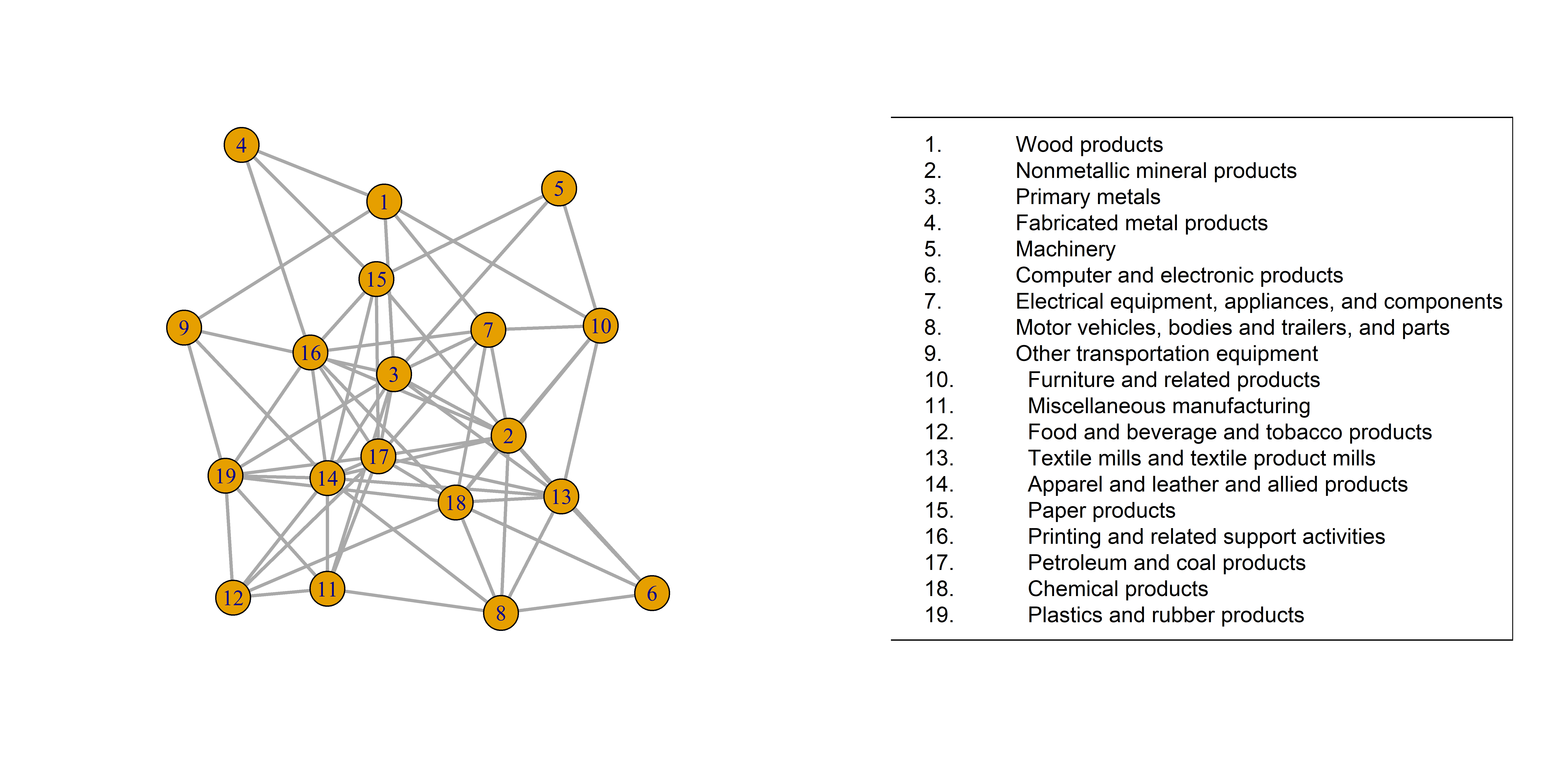
(a) Small ($p=19$)

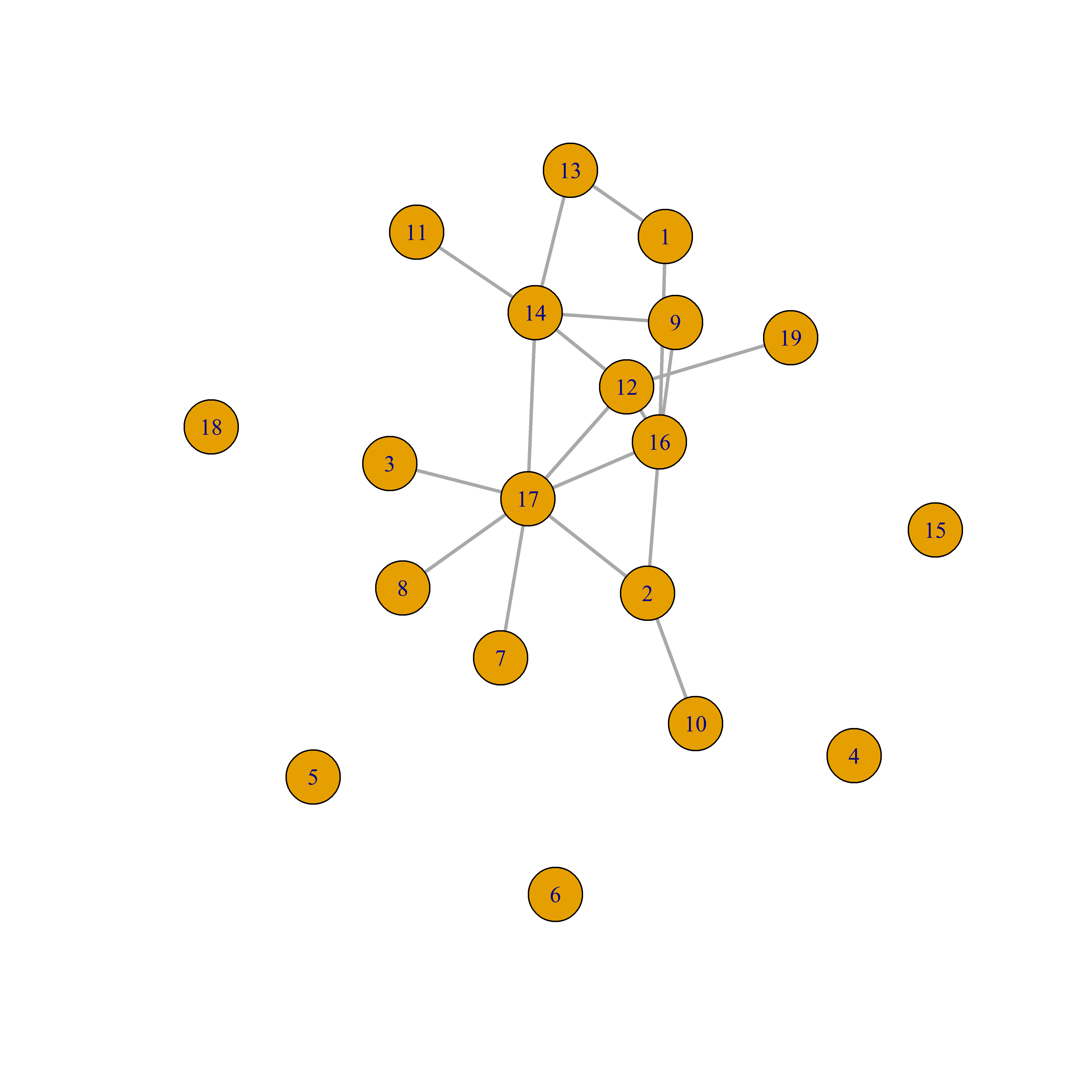
(b) Medium ($p=49$)

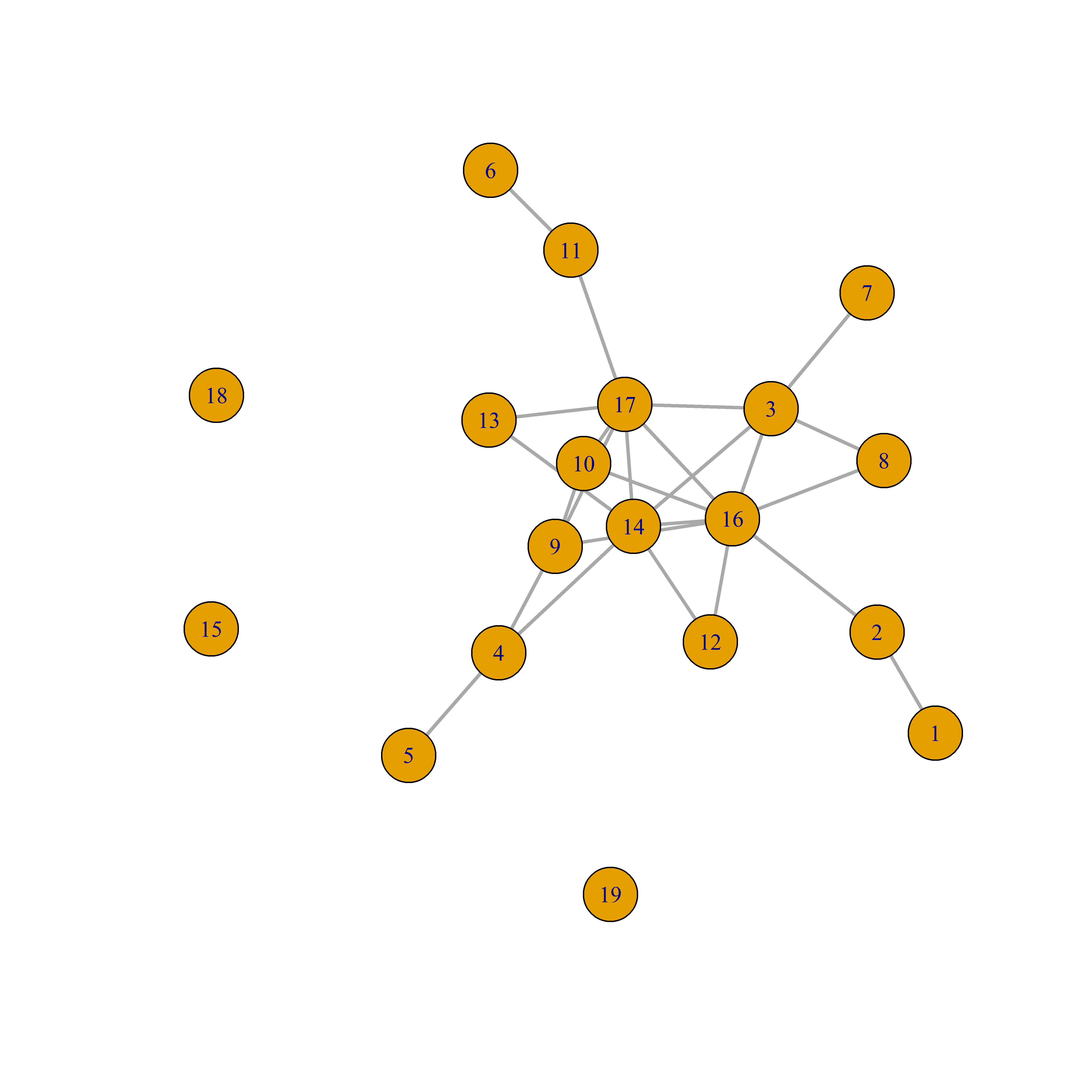
(c) Large ($p=66$)

7 Discussion

In this paper, we propose a novel multivariate time-series model that is amenable to estimating the conditional independence structure in the multivariate data at a given time point. We develop a Bayesian inference method along with computationally efficient posterior sampling steps. We further establish posterior contraction rates under the asymptotic regime that the number of time points and the dimension of the multivariate data go to infinity. The numerical performance of the proposed method is illustrated both in the synthetic data and for the components of the GDP. The marginal conditional independence structure helps to obtain several interesting interpretations for the GDP data.

Although we take a semiparametric approach in modeling the univariate time series, it would thus be interesting to consider parametric models such as AR, MA, or even ARMA for the latent univariate processes. We may then be able to make more explicit inference on features associated with the temporal dynamics. Another future direction is to adopt the proposed OUT model to address other types of structure learning problems for multivariate time series, such as learning a directed acyclic graphical (DAG) relation or dynamic graphical relation. Further structures can be imposed on the Cholesky parametrization. Future work will also consider establishing graph selection consistency results.

8 Proof of the main theorems

Proof of Theorem 1.

As in the proof of Theorem 8.19 of Ghosal and Van der Vaart (2017), (i) implies the evidence lower bound of the form $\int(q_{\theta}^{(T)}/q_{\theta_{0}}^{(T)})d\Pi(\theta)\geq e^{-DT\epsilon_{T}^{2}}$ with $p_{0}^{(T)}$-probability tending to one, for some constant $D>0$.

By Hölder’s inequality,

$$\int\phi_{T,j}p_{\theta_{0}}^{(T)}\leq\big{(}\int\phi_{T,j}q_{\theta_{0}}^{(T)}\big{)}^{(b-1)/b}\big{(}\int(p_{0}^{(T)}/q_{\theta_{0}}^{(T)}\big{)}^{b}q_{\theta_{0}}^{(T)})^{1/b}\leq e^{-K^{\prime}T\epsilon_{T}^{2}}G_{T}^{1/b}.$$

Now, for any $\theta\in\Theta_{T,j}^{*}$ such that $d_{T}(\theta,\theta_{0})>\epsilon$,

$$\mathrm{E}\int(1-\phi_{T,j})\frac{q_{\theta}^{T}}{q_{\theta_{0}}}\leq\big{(}\int(1-\phi_{T,j})q_{\theta}^{(T)}\big{)}^{(b-1)/b}\big{(}\int(p_{0}^{T}/q_{\theta_{0}}^{(T)}\big{)}^{b}q_{\theta}^{(T)})^{1/b}\leq e^{-K^{\prime}T\epsilon_{T}^{2}}G_{T}^{1/b},$$

where $K^{\prime}=K(b-1)/b$.

Now the proof can be completed by standard arguments by aggregating the tests to $\phi_{T}=\max\{\phi_{T,j}:j=1,\ldots,N_{T}\}$, since by the condition $\log G_{T}\lesssim T\epsilon_{T}^{2}$, the testing error rates are not affected. The argument goes through even though the more general Condition (iii) is assumed instead of the standard entropy condition for the sieve.

∎

Proof of Theorem 2.

We apply Theorem 1 with $p_{0}^{(T)}=p_{\mbox{\boldmath$\theta$}_{0}}^{(T)}$, the true density of the observations under the true parameter $\mbox{\boldmath$\theta$}_{0}$ for $\theta$ and $q_{\mbox{\boldmath$\theta$}}^{(T)}$ standing for the distribution of the observations under Whittle’s approximate distribution of a stationary time series. To verify Condition (i) of it, let $\bm{V}_{t}$ stand for the dispersion matrix of $\bm{W}_{*t}=(\bm{W}_{jt}:j=1,\ldots,p)$ under the true distribution in the time domain for $t=1,\ldots,T$. For $j=1,\ldots,p$, using Proposition 4.5.2 of Brockwell and Davis (1991), we have $\|\bm{F}^{T}\mbox{\boldmath$\Gamma$}_{j,T}\bm{F}-\mbox{\boldmath$\Lambda$}_{j,T}\|_{\infty}\lesssim T^{-1}$, where $\mbox{\boldmath$\Gamma$}_{j,T}$ is the true covariance in time-domain of $j$th univariate time-series and $\bm{F}$ is the Fourier basis matrix. Due to the assumed independence over $j$, for the marginal dispersion $\bm{V}_{t}$ will be a diagonal submatrix of $\mathrm{Diag}(\bm{F}^{T}\mbox{\boldmath$\Gamma$}_{1,T}\bm{F},\ldots,\bm{F}^{T}\mbox{\boldmath$\Gamma$}_{p,T}\bm{F})$. We thus have $\|\bm{V}_{t}-\bm{S}_{t}\|_{\infty}\lesssim T^{-1}$ and so $\|\bm{V}_{t}-\bm{S}_{t0}\|_{\mathrm{F}}\lesssim\sqrt{p}T^{-1}$. The true dispersion matrix of $\bm{X}_{t}$ is therefore $\bm{J}_{t}:=\bm{\Omega}_{0}^{-1/2}\bm{U}_{0}\bm{V}_{t}\bm{U}_{0}^{\rm T}\bm{\Omega}_{0}^{-1/2}$ and it satisfies $\|\bm{J}_{t}-\bm{M}_{t0}^{-1}\|_{\mathrm{F}}\leq\|\bm{\Omega}_{0}^{-1}\|_{\mathrm{op}}\|\bm{U}_{0}\|_{\mathrm{op}}^{2}\|\bm{V}_{t}-\bm{S}_{t0}\|_{\mathrm{F}}\lesssim\sqrt{p}T^{-1}$. Using (3.4), the actual true expectation of the log-likelihood ratio $\log q_{T}(\gamma_{0},\bm{X})-\log q_{T}(\gamma,\bm{X})$ is given by

$$-\frac{1}{2}\sum_{t=1}^{T}(\log\det\bm{M}_{t}-\log\det\bm{M}_{t0})+\frac{1}{2}\sum_{t=1}^{T}\mathrm{tr}((\bm{M}_{t}-\bm{M}_{t0})\bm{J}_{t})$$

$$=\frac{1}{2}\sum_{t=1}^{T}[-\log\det(\bm{I}_{p}+\bm{R}_{t})+\mathrm{tr}(\bm{R}_{t})]+\mathrm{tr}[(\bm{M}_{t}-\bm{M}_{t0})(\bm{J}_{t}-\bm{M}_{t0}^{-1})],$$

where $\bm{R}_{t}=\bm{M}_{t0}^{-1}(\bm{M}_{t}-\bm{M}_{t0})$. Using the Cauchy-Schwarz inequality for matrices, namely $|\mathrm{tr}(\bm{A}\bm{B})|\leq\|\bm{A}\|_{\mathrm{F}}\|\bm{B}\|_{\mathrm{F}}$, it follows that $\mathrm{tr}[(\bm{M}_{t}-\bm{M}_{t0})(\bm{J}_{t}-\bm{M}_{t0}^{-1})]\leq\|\bm{M}_{t}-\bm{M}_{t0}\|_{\mathrm{F}}\times\sqrt{p^{2}}T^{-1}\leq\epsilon_{T}^{3}\leq\epsilon_{T}^{2}$, whenever $\max_{i}\|\bm{M}_{t}-\bm{M}_{t0}\|_{\mathrm{F}}\leq\epsilon_{T}$. Thus the last term in the display can be bounded by $T\epsilon_{T}^{2}$. With $\rho_{1},\ldots,\rho_{p}$ standing for the eigenvalues of $\bm{R}_{t}$, the expression in the sum inside the first term can be written as $-\log(1+\rho_{j})+\rho_{j}\leq\rho_{j}^{2}$ whenever $|\rho_{j}|\leq 1/2$. The condition is ensured if $\max_{t}\|\bm{M}_{t}-\bm{M}_{t0}\|_{\mathrm{F}}\leq\epsilon_{T}$. Hence the expression in the display can be bounded by a constant multiple of $T\epsilon_{T}^{2}$ if $\max_{t}\|\bm{M}_{t}-\bm{M}_{t0}\|_{\mathrm{F}}\leq\epsilon_{T}$. The negative logarithm of the prior probability of the last event is bounded by a constant multiple of $T\epsilon_{T}^{2}$ by Lemma 6. This completes the verification of Condition (i).

The verification of Conditions (ii), (iii), and (iv) of Theorem 1 is detailed in Lemma  8. Finally, by Lemma 1, it follows that the logarithm of the integral in (4.3) is bounded by a multiple of $p\lesssim T\epsilon_{T}^{2}$. This completes the proof of Assertion (1) for the metric $d$ given by $d^{2}(\mbox{\boldmath$\gamma$},\mbox{\boldmath$\gamma$}_{0})=T^{-1}\sum_{t=1}^{T}\min(\|\bm{M}_{t}-\bm{M}_{t0}\|_{\mathrm{F}}^{2},c_{0})$. Thus Assertion (1) holds.

The proof of Assertion (2) is similar using the second part of Lemma 8. ∎

Proof of Theorem 3.

It follows from the proof of Lemma 2, if all eigenvalues of $\bm{M}_{t0}^{-1/2}\bm{M}_{t}\bm{M}_{0i}^{-1/2}$ lie within a fixed compact set not depending on $\bm{M}_{t}$, $t=1,\ldots,T$, then the minimum operation appearing in the estimates (4.6) and (4.8) can be removed, and consequently, so is the case for Lemmas 7 and 8, and ultimately in Theorem 2, by choosing $c_{0}>0$ sufficiently large. This immediately gives Assertions (a) and (b).

To prove (c), we observe that (b) implies that $\|T^{-1}\sum_{t=1}^{T}\bm{M}_{t}^{-1}-T^{-1}\sum_{t=1}^{T}\bm{M}_{t0}^{-1}\|_{\mathrm{F}}\leq m_{T}\epsilon_{T}$ with posterior probability arbitrarily close to one under the true distribution. Due to the integrability condition, we have that uniformly for all spectral densities $f_{1},\ldots,f_{j}$ taking values in a compact interval, $T^{-1}\sum_{t=1}^{T}|f_{j}(\omega_{k(i)})-\int f_{j}(\omega)d\omega|=O(T^{-1})$. Together with the identifiability condition that $\int f_{j}(\omega)d\omega=1$ for $j=1,\ldots,p$, uniformly for all spectral densities $f_{1},\ldots,f_{j}$ taking values in that compact interval,

$$\|T^{-1}\sum_{t=1}^{T}\bm{S}_{t}-\bm{I}_{p}\|_{\mathrm{F}}=O(\sqrt{p}/T),$$ (8.1)

resulting in the convergence

$$\|T^{-1}\sum_{t=1}^{T}\bm{M}_{t}^{-1}-\bm{\Sigma}\|_{\mathrm{F}} =\|\bm{\Omega}^{-1/2}\bm{U}(T^{-1}\sum_{t=1}^{T}\bm{S}_{t}-\bm{I}_{p})\bm{U}^{\rm T}\bm{\Omega}^{-1/2}\|_{\mathrm{F}}$$

$$\leq\|\bm{\Omega}^{-1}\|_{\mathrm{op}}\|T^{-1}\sum_{t=1}^{T}\bm{S}_{t}-\bm{I}_{p}\|_{\mathrm{F}},$$

which is $O(\sqrt{p}/T)=o(\epsilon_{T})$. Since the true value also satisfies the above bound, in particular, it follows from the triangle inequality that $\|\bm{\Sigma}-\bm{\Sigma}_{0}\|_{\mathrm{F}}\leq m_{T}(1+o(1))\epsilon_{T}$ with posterior probability arbitrarily close to one under the true distribution, proving Assertion (c).

Finally, Assertion (d) is obtained from Assertion (c) using the relation $\bm{\Omega}-\bm{\Omega}_{0}=\bm{\Sigma}^{-1}(\bm{\Sigma}-\bm{\Sigma}_{0})\bm{\Sigma}_{0}^{-1}$ which gives the inequality $\|\bm{\Omega}-\bm{\Omega}_{0}\|_{\mathrm{F}}\leq\|\bm{\Sigma}^{-1}\|_{\mathrm{op}}\|\bm{\Sigma}-\bm{\Sigma}_{0}\|_{\mathrm{F}}\|\bm{\Sigma}_{0}^{-1}\|_{\mathrm{op}}$, and the fact that the closeness of $\bm{\Sigma}$ and $\bm{\Sigma}_{0}$ in the Frobenius norm implies their closeness in the operator norm leading to the conclusion that the eigenvalues of $\bm{\Sigma}$ lie between two positive numbers since $\bm{\Sigma}_{0}$ has this property by Assumption (A1). ∎

9 Proof of the auxiliary results

Proof of Proposition 1.

The first relation is immediate from the OUT representation (2.1), the orthogonality of $\bm{U}$ and $\mathrm{D}(\bm{Z}_{t})=\bm{I}_{p}$, since $\mathrm{D}(\bm{Y}_{t})=\bm{\Sigma}^{1/2}\bm{U}\bm{I}_{p}\bm{U}^{\rm T}\bm{\Sigma}^{1/2}=\bm{\Sigma}$.

The relation (ii) follows from the OUT representation (2.1) that

$$\mbox{\boldmath$\Gamma$}(h,t;\bm{Y})=\bm{\Sigma}^{-1/2}\bm{\Sigma}^{1/2}\bm{U}\mathrm{E}(\bm{Z}_{t}\bm{Z}_{t+h}^{\rm T})\bm{U}^{\rm T}\bm{\Sigma}^{1/2}\bm{\Sigma}^{-1/2}=\bm{U}\mathrm{E}(\bm{Z}_{t}\bm{Z}_{t+h}^{\rm T})\bm{U}^{\rm T},$$ (9.1)

which is symmetric because $\mathrm{E}(\bm{Z}_{t}\bm{Z}_{t+h}^{\rm T})$ is a diagonal matrix due to the independence of the component series.

As shown in the proof of (ii), $\mbox{\boldmath$\Gamma$}(h,t;\bm{Y})=\bm{U}\mathrm{Diag}(\gamma_{j}(h,t):j=1,\ldots,p)\bm{U}^{\rm T}$, so the rows of the orthogonal matrix $\bm{U}$ are the eigenvectors, which do not vary with $h$ or $t$. It also follows that $\{\gamma_{j}(h,t):j=1,\ldots,p\}$ are the set of eigenvalues. If all latent processes are stationary, the eigenvalues depend only on the lag $h$.

To prove covariance-stationarity (respectively, strict stationarity under the additional Gaussianity assumption) and zero trends, it suffices to check that $\mathrm{E}(\bm{Y}_{t}\bm{Y}_{t+h}^{\rm T})$ is free from $t$ if all latent processes $(Z_{j,t}:t=1,2,\ldots)$, $j=1,\ldots,p$ are stationary. This is immediate from the OUT representation since $\mathrm{E}(\bm{Y}_{t}\bm{Y}_{t+h}^{\rm T})=\bm{\Sigma}^{1/2}\bm{U}\bm{S}_{h}\bm{U}^{\rm T}(\bm{R}^{-1})^{\rm T}$, where $\bm{S}_{h}=\mathrm{E}(\bm{Y}_{t}\bm{Y}_{t+h}^{\rm T})$.

Finally, to prove that $\bm{Y}_{t}$ is causal when all $Z_{j,t}$, $j=1,\ldots,p$, are causal. By the assumption, there exist functions $H_{j,t}$, $j=1,\ldots,p$, $t=1,2,\ldots$, such that $Z_{j,t}=H_{j,t}(e_{j,t},e_{j,t-1},\ldots)$ for independent random variables $\{e_{j,s}:s=t,t-1,\ldots\}$, for all $j=1,\ldots,p$. Then defining $\bm{e}_{t}=(e_{j,t}:j=1,\ldots,p)$ and $\bm{H}_{t}(\bm{e}_{t},\bm{e}_{t-1},\ldots)=\bm{R}^{-1}\bm{U}(H_{j,t}(e_{j,t},e_{j,t-1},\ldots):j=1,\ldots,p)^{\rm T}$, we have that $\bm{Y}_{t}=\bm{H}_{t}(\bm{e}_{t},\bm{e}_{t-1},\ldots)$ for all $t$, proving the assertion. ∎

Proof of Lemma 1.

First, we show that the $b$th moment of the likelihood ratio is indeed finite. It is enough to show finiteness for each $j$ since the density factorizes due to independence over $j$. For any $j$

$$\frac{\phi_{T}(\bm{W}_{j*};\bm{0},\bm{F}^{\rm T}\mbox{\boldmath$\Gamma$}_{j,T}\bm{F})^{b}}{\phi_{T}(\bm{W}_{j*};\bm{0},\mbox{\boldmath$\Lambda$}_{j,T})^{b}}=\frac{\det(\bm{F}^{\rm T}\mbox{\boldmath$\Gamma$}^{-1}_{j,T}\bm{F})^{b/2}}{\det(\mbox{\boldmath$\Lambda$}^{-1}_{j,T})^{b/2}}\exp(-\frac{b}{2}\bm{W}_{j*}^{\rm T}[\bm{F}^{\rm T}\mbox{\boldmath$\Gamma$}^{-1}_{j,T}\bm{F}-\mbox{\boldmath$\Lambda$}^{-1}_{j,T}]\bm{W}_{j*}).$$

Thus, for finiteness of the $b$th moment of the likelihood ratio we would need positive definiteness of $\bm{B}_{j}=b[\bm{F}^{\rm T}\mbox{\boldmath$\Gamma$}^{-1}_{j,T}\bm{F}-\mbox{\boldmath$\Lambda$}^{-1}_{j,T}]+\mbox{\boldmath$\Lambda$}^{-1}_{j,T}=b\bm{F}^{\rm T}\mbox{\boldmath$\Gamma$}^{-1}_{j,T}\bm{F}-(b-1)\mbox{\boldmath$\Lambda$}^{-1}_{j,T}]$. Since $\mbox{\boldmath$\Gamma$}^{-1}_{j,T}$ is the finite Toeplitz form defined based on $f_{j}$, by the result 5.2 (b) of Grenander and Szegø (1984) we the the eigenvalues of $b\bm{F}^{\rm T}\mbox{\boldmath$\Gamma$}^{-1}_{j,T}\bm{F}$ are bounded in the interval $[bc_{2j}^{-1},bc_{1j}^{-1}]$. Similarly, the eigenvalues of $(b-1)\mbox{\boldmath$\Lambda$}^{-1}_{j,T}$ are bound in the interval $[(b-1)c_{2j}^{-1},(b-1)c_{1j}^{-1}].$ using the fact that for two positive definite matrices $\bm{A}_{1},\bm{A}_{2}$, the difference $\bm{A}_{1}-\bm{A}_{2}$ is positive definite if the minimum eigenvalue of $\bm{A}_{1}$ is strictly bigger than the maximum eigenvalue of $\bm{A}_{2}$, a sufficient condition for $\bm{B}_{j}$ to be positive definite is that

$$bc_{2j}^{-1}>(b-1)c_{1j}^{-1},\quad\mbox{that is},\quad 1<b<\frac{c_{1j}^{-1}}{c_{1j}^{-1}-c_{2j}^{-1}}=\frac{c_{2j}}{c_{2j}-c_{1j}}.$$ (9.2)

Thus, with the choice $b=(1+\min_{j}\frac{c_{2j}}{c_{2j}-c_{1j}})/2$, the requirement is met. Also by the asymptotic refinement theorem for functions of eigenvalues of Toeplitz forms, (Grenander and Szegø (1984), page 76), and the error rate of discrete approximation of Riemann integrals, we have

$$\frac{\det(\bm{F}^{\rm T}\mbox{\boldmath$\Gamma$}^{-1}_{j,T}\bm{F})^{b/2}}{\det(\mbox{\boldmath$\Lambda$}^{-1}_{j,T})^{b/2}}=\psi_{j}+O(T^{-1}),$$ (9.3)

where $\psi_{j}$ is a finite constant defined in the theorem. Then completing the integral we have the value of the integral as

$$G_{T}=\prod_{j=1}^{p}(\psi_{j}+O(T^{-1})\exp\{-\log\det(b\bm{F}^{\rm T}\mbox{\boldmath$\Gamma$}^{-1}_{j,T}\bm{F}\mbox{\boldmath$\Lambda$}_{j,T}-(b-1)\bm{I})\}.$$ (9.4)

Writing $\eta_{j,t}$s for the eigenvalues of $\bm{F}^{\rm T}\mbox{\boldmath$\Gamma$}^{-1}_{j,T}\bm{F}\mbox{\boldmath$\Lambda$}_{j,T}$, we have

$$\log\det(b\bm{F}^{\rm T}\mbox{\boldmath$\Gamma$}^{-1}_{j,T}\bm{F}\mbox{\boldmath$\Lambda$}_{j,T}-(b-1)\bm{I})=\log\det(b(\bm{F}^{\rm T}\mbox{\boldmath$\Gamma$}^{-1}_{j,T}\bm{F}\mbox{\boldmath$\Lambda$}_{j,T}-\bm{I})+\bm{I})$$

$$\quad=\sum_{t=1}^{T}\log\{b(\eta_{j,t}-1)+1\},$$

where, by the positive definiteness of $\bm{B}_{j}$, $b(\eta_{j,t}-1)>-1.$ From Lemma A1 of Choudhuri et al. (2004b), we have $|\log\det(\bm{F}^{\rm T}\mbox{\boldmath$\Gamma$}_{j,T}\bm{F})-\log\det(\mbox{\boldmath$\Lambda$}_{j,T})|=O(1)$. Moreover, Lemma A2 of Choudhuri et al. (2004b) implies $\sum_{t}(\eta_{j,t}-1)^{2}$ and $\sum_{t}(\eta_{j,t}-1)$ are uniformly bounded for all $T$. Hence, it leads to $|\log\det(b\bm{F}^{\rm T}\mbox{\boldmath$\Gamma$}^{-1}_{j,T}\bm{F}\mbox{\boldmath$\Lambda$}_{j,T}-(b-1)\bm{I})|=O(1).$ Therefore we have $\log G_{T}\asymp p$. ∎

Proof of Lemma 2.

Let $\bm{R}=\bm{\Omega}_{1}^{-1/2}(\bm{\Omega}_{2}-\bm{\Omega}_{1})\bm{\Omega}_{1}^{-1/2}$ and let $\rho_{1},\ldots,\rho_{p}$ be the eigenvalues of $\bm{R}$.

The equalities in (4.6) and (4.7) follow from straightforward integration of normal densities.

To prove the inequality in (4.6), we write the expression as $\exp\{\frac{1}{4}\sum_{j=1}^{p}(\log(1+\rho_{j})-2\log(1+\rho_{j}/2))\}$. The function $h(x)=\log(1+x)-2\log(1+x/2)$ has a maximum $0$ at $x=0$, and is decreasing thereafter. Thus for any chosen $c>0$, taking $c_{2}=-h(c)/c^{2}>0$, it follows that $h(x)\leq c_{2}x^{2}$ for all $0\leq x\leq c$, while for $x>c$, $h(x)\leq h(c)=-c_{2}c^{2}$. On the interval $(-1,1]$, $h(x)\leq-x^{2}/72$ by a second-order Taylor expansion and the fact that $h^{\prime\prime}(x)$ attains its maximum value $-1/72$ at $x=1$ on this interval. Then $\max(h(x),c_{1})\leq-c_{2}\min(x^{2},c_{1})$, where $c_{2}$ can be taken to be $\min(-h(c)/c^{2},1/72)$ and $c_{1}=\max(-h(c),1)$. It is also clear that $c_{1}$ can be taken arbitrarily large by choosing $c$ large enough since $h(x)\to-\infty$ as $x\to\infty$. Thus the expression in (4.6) is bounded by

$$\exp\{-c_{2}\sum_{j=1}^{p}\min(\rho_{j}^{2},c_{1})\}\leq\exp\{-\min(\sum_{j=1}^{p}\rho_{j}^{2},c_{1})/72\}=\exp\{-c_{2}\min(\|\bm{R}\|_{\mathrm{F}}^{2},c_{1})\}.$$

Finally, applying the Frobenius-operator norm inequality on the relation $\bm{\Omega}_{2}-\bm{\Omega}_{1}=\bm{\Omega}_{1}^{1/2}\bm{R}\bm{\Omega}_{1}^{1/2}$, we get the estimate $\|\bm{R}\|_{\mathrm{F}}\geq\|\bm{\Omega}_{2}-\bm{\Omega}_{1}\|_{\mathrm{F}}/\|\bm{\Omega}_{1}\|_{\mathrm{op}}$. Substituting in the last inequality, the assertion is established.

For the inequality in (4.8), writing the expression as $\exp\{\frac{1}{2}\sum_{j=1}^{p}(2\log(1+\rho_{j})-\log(1+2\rho_{j}))\}$ and noting that the function $h(x)=2\log(1+x)-\log(1+2x)$ has a minimum $0$ at $x=0$, $h$ is convex and $h^{\prime\prime}(x)\leq 30$ for $|x|\leq 1/3$, we can bound the expression in (4.7) by $\exp\{15\sum_{j=1}^{p}\rho_{j}^{2}\}=\exp\{15\|\bm{R}\|_{\mathrm{F}}^{2}\}$ whenever $\|\bm{R}\|_{\mathrm{F}}\leq 1/3$. Because $\|\bm{R}\|_{\mathrm{F}}\leq\|\bm{\Omega}_{1}^{-1}\|_{\mathrm{op}}\|\bm{\Omega}_{2}-\bm{\Omega}_{1}\|_{\mathrm{F}}$ by the Frobenius-operator norm inequality, the assertion follows.

The proofs of the relations (4.8) and (4.9) respectively follow those of (4.6) and (4.7) with the key observation that $\bm{R}$ can be alternatively expressed as $\bm{R}=-\bm{\Omega}_{1}^{1/2}(\bm{\Omega}_{2}^{-1}-\bm{\Omega}_{1}^{-1})\bm{\Omega}_{1}^{1/2}$. ∎

Proof of Lemma 3.

First, to show that the eigenvalues are bounded above, we uniformly bound the operator norms $\|\bm{M}_{t0}\|_{\mathrm{op}}$. Observe that

$$\|\bm{M}_{t0}\|_{\mathrm{op}} =\|\bm{\Sigma}_{0}^{1/2}\bm{U}_{0}\bm{S}_{t}^{-1}\bm{U}_{0}^{\rm T}\bm{\Sigma}_{0}^{1/2}\|_{\mathrm{op}}$$

$$\quad\leq\|\bm{\Sigma}_{0}\|_{\mathrm{op}}\|\bm{S}_{t}^{-1}\|_{\mathrm{op}}\leq\|\bm{\Sigma}_{0}\|_{\mathrm{op}}\max\{1/f_{j0}(\omega_{k(i)}):1\leq j\leq p\},$$

which is bounded uniformly in $i$ by Assumptions (A1) and (A3), since $\|\bm{U}_{0}\|_{\mathrm{op}}=1$, as all eigenvalues of the orthogonal matrix $\bm{U}_{0}$ lie on the unit circle in the complex plane.

To show that the eigenvalues are lower-bounded by a positive constant, it suffices to upper bound the operator norm of the inverse:

$$\|\bm{M}_{t0}^{-1}\|_{\mathrm{op}} =\|\bm{\Sigma}_{0}^{-1/2}\bm{U}_{0}\bm{S}_{t}\bm{U}_{0}^{\rm T}\bm{\Sigma}_{0}^{-1/2}\|_{\mathrm{op}}$$

$$\quad\leq\|\bm{\Sigma}_{0}^{-1}\|_{\mathrm{op}}\|\bm{S}_{t}\|_{\mathrm{op}}\leq\|\bm{\Sigma}_{0}^{-1}\|_{\mathrm{op}}\max\{f_{j0}(\omega_{k(i)}):1\leq j\leq p\},$$

which is also bounded uniformly in $i$ by Assumptions (A1) and (A3), and the orthogonality of $\bm{U}_{0}$. ∎

Proof of Lemma 4.

For $\bm{U}_{1}=(\bm{I}_{p}-\bm{A}_{1})(\bm{I}_{p}+\bm{A}_{1})^{-1}$, $\bm{U}_{2}=(\bm{I}_{p}-\bm{A}_{2})(\bm{I}_{p}+\bm{A}_{1})^{-1}$, observe that

$$\|(\bm{I}_{p}-\bm{A}_{1})(\bm{I}_{p}+\bm{A}_{1})^{-1}-(\bm{I}_{p}-\bm{A}_{2})(\bm{I}_{p}+\bm{A}_{2})^{-1}\|_{\mathrm{F}}$$

$$\quad\leq\|\bm{A}_{1}-\bm{A}_{2}\|_{\mathrm{F}}\|(\bm{I}_{p}+\bm{A}_{1})^{-1}\|_{\mathrm{op}}+\|\bm{I}_{p}-\bm{A}_{2}\|_{\mathrm{op}}\|(\bm{I}_{p}+\bm{A}_{1})^{-1}-(\bm{I}_{p}+\bm{A}_{1})^{-1}\|_{\mathrm{F}}$$

$$\quad\leq\|\bm{A}_{1}-\bm{A}_{2}\|_{\mathrm{F}}\|(\bm{I}_{p}+\bm{A}_{1})^{-1}\|_{\mathrm{op}}[1+\|\bm{I}_{p}-\bm{A}_{2}\|_{\mathrm{op}}]\|(\bm{I}_{p}+\bm{A}_{2})^{-1}\|_{\mathrm{op}}.$$

As $\bm{A}_{1}$, $\bm{A}_{2}$ are skew-symmetric matrices, all its non-zero eigenvalues are purely imaginary. Thus any eigenvalue of $(\bm{I}_{p}+\bm{A}_{1})^{-1}$ or $(\bm{I}_{p}+\bm{A}_{2})^{-1}$, being of the form $(1+ia)^{-1}$, is bounded above in absolute value by $1$. Further, $\|\bm{I}_{p}-\bm{A}_{2}\|_{\mathrm{op}}^{2}\leq\|\bm{I}_{p}-\bm{A}_{2}\|_{\mathrm{F}}^{2}\leq p+p(p-1)B^{2}$. Substituting these estimates, the conclusion follows.

∎

Proof of Lemma 5.

By the applications of the matrix norm inequalities and observing the fact that $\|\bm{I}_{p}-\bm{L}_{1}\|_{\mathrm{op}}=1=\|\bm{I}_{p}-\bm{L}_{2}\|_{\mathrm{op}}$, we have

$$\|(\bm{I}_{p}-\bm{L}_{1})\bm{D}^{2}_{1}(\bm{I}_{p}-\bm{L}_{1}^{\rm T})-(\bm{I}_{p}-\bm{L}_{2})\bm{D}^{2}_{2}(\bm{I}_{p}-\bm{L}_{2}^{\rm T})\|_{\mathrm{F}}$$

$$\leq\|\bm{L}_{1}-\bm{L}_{2}\|_{\mathrm{F}}\|\bm{D}_{1}\|_{\mathrm{op}}^{2}+\|\bm{D}^{2}_{1}-\bm{D}^{2}_{2}\|_{\mathrm{F}}+\|\bm{D}_{2}\|_{\mathrm{op}}^{2}\|\bm{L}_{1}-\bm{L}_{2}\|_{\mathrm{F}}.$$

Since $\bm{D}_{1},\bm{D}_{2}$ are diagonal matrices with entries in $(0,B)$, the result is immediate.

∎

Proof of Lemma 6.

First we show that for $\epsilon>0$ sufficiently small, if $\|\bm{\Omega}-\bm{\Omega}_{0}\|_{\mathrm{F}}\leq\epsilon$, $\|\bm{U}-\bm{U}_{0}\|_{\mathrm{F}}<\epsilon$, $\max\{\|\bm{S}_{t}-\bm{S}_{t0}\|_{\mathrm{F}}<\epsilon$, then for some constant $C_{0}$ depending on the true parameters $\bm{\Omega}_{0}$, $\bm{U}_{0}$ and $f_{10},\ldots,f_{j0}$, the relation $\max\{\|\bm{M}_{t}-\bm{M}_{t0}\|_{\mathrm{F}}:1\leq t\leq T\}\leq C_{0}\epsilon$ holds.

To prove this, we recall the facts that $\|\bm{\Omega}_{0}\|_{\mathrm{op}}$ and $\|\bm{S}_{t}^{-1}\|_{\mathrm{op}}$, $t=1,\ldots,T$, are uniformly bounded by Assumptions (A1) and (A3), and that $\|\bm{U}_{0}\|_{\mathrm{op}}=1$. This implies that if $\epsilon>0$ is sufficiently small and if $\|\bm{\Omega}-\bm{\Omega}_{0}\|_{\mathrm{F}}\leq\epsilon$, $\|\bm{U}-\bm{U}_{0}\|_{\mathrm{F}}<\epsilon$, $\max\{\|\bm{S}_{t}-\bm{S}_{t0}\|_{\mathrm{F}}<\epsilon$, then $\|\bm{\Omega}_{0}\|_{\mathrm{op}}$ and $\|\bm{S}_{t}^{-1}\|_{\mathrm{op}}$, $t=1,\ldots,T$ are also uniformly bounded, and $\|\bm{U}\|_{\mathrm{op}}=1$ by the orthogonality of $\bm{U}$. Next, we argue that if $\|\bm{\Omega}-\bm{\Omega}_{0}\|_{\mathrm{F}}\leq\epsilon$, then $\|\bm{\Omega}^{1/2}-\bm{\Omega}_{0}^{1/2}\|_{\mathrm{F}}\lesssim\epsilon$. To see this, let $e_{1},\ldots,e_{p}$ be the eigenvalues of the positive definite matrix $\bm{\Omega}_{0}^{-1/2}\bm{\Omega}\bm{\Omega}_{0}^{-1/2}$. Then by the Frobenius-operator norm inequality $\|\bm{A}\bm{B}\|_{\mathrm{F}}\leq\|\bm{A}\|_{\mathrm{op}}\|\bm{B}\|_{\mathrm{F}}$ or $\|\bm{A}\bm{B}\|_{\mathrm{F}}\leq\|\bm{A}\|_{\mathrm{F}}\|\bm{B}\|_{\mathrm{op}}$ and Assumption (A1), $\|\bm{\Omega}^{1/2}-\bm{\Omega}_{0}^{1/2}\|_{\mathrm{F}}^{2}\lesssim\|\bm{\Omega}_{0}^{-1/4}\bm{\Omega}^{1/2}\bm{\Omega}_{0}^{-1/4}-\bm{I}_{p}\|_{\mathrm{F}}^{2}=\sum_{j=1}^{p}(\sqrt{e_{j}}-1)^{2}$. Now if $\|\bm{\Omega}-\bm{\Omega}_{0}\|_{\mathrm{F}}$ is sufficiently small, then so is $\|\bm{\Omega}_{0}^{-1/2}\bm{\Omega}\bm{\Omega}_{0}^{-1/2}-\bm{I}_{p}\|_{\mathrm{F}}^{2}=\sum_{j=1}^{p}({e_{j}}-1)^{2}$, and hence all eigenvalues $e_{1},\ldots,e_{p}$ lie in a sufficiently small neighborhood of $1$. Therefore, $\sum_{j=1}^{p}(\sqrt{e_{j}}-1)^{2}$ can be bounded by a constant multiple of $\sum_{j=1}^{p}({e_{j}}-1)^{2}$. Thus $\|\bm{\Omega}^{1/2}-\bm{\Omega}_{0}^{1/2}\|_{\mathrm{F}}\lesssim\|\bm{\Omega}-\bm{\Omega}_{0}\|_{\mathrm{F}}$.

By repeatedly applying the triangle inequality and the Frobenius-operator norm inequality, and using the above estimates, we obtain the estimate

$$\|\bm{M}_{t}-\bm{M}_{t0}\|_{\mathrm{F}} \lesssim\max\{\|\bm{\Omega}_{t}^{1/2}-\bm{\Omega}_{t0}^{1/2}\|_{\mathrm{F}},\|\bm{U}-\bm{U}_{0}\|_{\mathrm{F}},\|\bm{S}_{t}^{-1}-\bm{S}_{t0}^{-1}\|_{\mathrm{F}}\}$$

$$\lesssim\max\{\|\bm{\Omega}_{t}-\bm{\Omega}_{t0}\|_{\mathrm{F}},\|\bm{U}-\bm{U}_{0}\|_{\mathrm{F}},\|\bm{S}_{t}^{-1}-\bm{S}_{t0}^{-1}\|_{\mathrm{F}}\}$$ (9.5)

uniformly for $t=1,\ldots,T$. Then, using the prior independence of the parameters, it will suffice to show that for all sufficiently small $\epsilon>0$,

1. $-\log\Pi(\|\bm{\Omega}-\bm{\Omega}_{0}\|_{\mathrm{F}}\leq\epsilon)\lesssim(p+s)\log(p/\epsilon)$;

2. $-\log\Pi(\|\bm{U}-\bm{U}_{0}\|_{\mathrm{F}}\leq\epsilon)\lesssim(p+s)\log(p/\epsilon)$;

3. $-\log\Pi(\max\{\|\bm{S}_{t}^{-1}-\bm{S}_{t0}^{-1}\|_{\mathrm{F}}:1\leq t\leq p\}\leq\epsilon)\lesssim(p+\epsilon^{-1/\alpha})\log(1/\epsilon)$ for $K\asymp\epsilon^{-1/\alpha}$.

The bound in (i) was established in the proof of Theorem 4.2 of Shi et al. (2021) for the sparse Cholesky decomposition prior for $\bm{\Omega}$ based on independent continuous shrinkage distributions on the entries of $\bm{L}$; the proof using a hard-spike-and-slab distribution on the entries is analogous and is slightly simpler.

To show the estimate in (ii), in view of Lemma 4, it suffices to show that $-\log\Pi(\|\bm{A}-\bm{A}_{0}\|_{\mathrm{F}}\leq\epsilon/p)\lesssim s\log(p/\epsilon)$. There are $p(p-1)/2$ unrestricted entries in $\bm{A}$, out of which $\bm{A}_{0}$ has $s$ non-zero entries. A standard probability estimate (see, eg., Example 2.2 of Castillo and Van Der Vaart (2012)) now establishes the bound when the slab probability decays polynomially in $p$.

To establish the bound in (iii), since the true spectral densities are bounded away from $0$, it suffices to prove that $-\log\Pi(\max\{\|f_{t}-f_{t0}\|_{\infty}:1\leq t\leq p\}\leq\epsilon)\lesssim(p+\epsilon^{-1/\alpha})\log(1/\epsilon)$. In view of (4.5), it suffices to use $K\asymp\epsilon^{-1/\alpha}$ terms in the B-spline basis expansion to control the bias within a multiple of $\epsilon$. Hence, using the fact that the normalized B-splines are uniformly bounded by a multiple of $K$, it will be enough to estimate the prior concentration of the $\epsilon/K$ neighborhoods of a $R(p+K)$-dimensional vector of uniformly bounded entries in the Euclidean distance. The resulting estimate is $(\epsilon/K)^{R(p+K)}$. Since $R$ is assumed to be not growing with $T$, this leads to (iii).

The result follows from these estimates as $\epsilon_{T}=\sqrt{\max\{(p+s),T^{-\alpha/(2\alpha+1})\}(\log T)/T}$ satisfies $(p+s)\log(p/\epsilon)+(p+\epsilon^{-1/\alpha})\lesssim T\epsilon^{2}$. ∎

Proof of Lemma 7.

Let $\phi_{T}=\mathbbm{1}\{\prod_{t=1}^{T}\phi_{p}(\bm{X}_{t};\bm{0},\bm{M}_{t1}^{-1})/\phi_{p}(\bm{X}_{t};\bm{0},\bm{M}_{t0}^{-1})>1\}$ stand for the likelihood ratio test for testing the simple null $\bm{X}_{t}\sim\mathrm{N}_{p}(\bm{0},\bm{M}_{t0}^{-1})$ for all $t=1,\ldots,T$, independently, against the point alternative $\bm{X}_{t}\sim\mathrm{N}_{p}(\bm{0},\bm{M}_{t1}^{-1})$, for all $t=1,\ldots,T$, independently. Then by Markov’s inequality, Lemma 3 and the first assertion of Lemma 2

$$\int\phi_{T}d\mathrm{N}_{p}(\bm{0},\bm{M}_{t0}^{-1}) \leq\prod_{t=1}^{T}\int\sqrt{\phi_{p}(\bm{x}_{t};\bm{0},\bm{M}_{t1}^{-1})}\sqrt{\phi_{p}(\bm{x};\bm{0},\bm{M}_{t0}^{-1})}d\bm{x}_{t}$$

$$\quad\leq e^{-c_{0}^{\prime}\sum_{t=1}^{T}\min(\|\bm{M}_{t1}-\bm{M}_{t0}\|_{\mathrm{F}}^{2},c_{1})}$$

where $c_{0},c_{0}^{\prime}>0$ depend on $c_{1},c_{2}$ in Lemma 2 and $b_{1},b_{2}$, and that $c_{0}$ can be chosen as large as we please at the expense of making $c_{2}^{\prime}$ smaller. Hence the first assertion follows with $K_{0}=c_{0}^{\prime}$.

By symmetry, it follows that $\int(1-\phi_{T})d\mathrm{N}_{p}(\bm{0},\bm{M}_{t1}^{-1})\leq e^{-c\epsilon^{2}}$ as well. Now by the Cauchy-Schwarz inequality and the estimate in the second assertion of Lemma 2,

$$\int(1-\phi_{T})d\mathrm{N}_{p}(\bm{0},\bm{M}_{t2}^{-1})$$

$$\leq\big{(}\int(1-\phi_{T})d\mathrm{N}_{p}(\bm{0},\bm{M}_{t1}^{-1})\big{)}^{1/2}\prod_{t=1}^{T}\big{(}\int\big{(}\frac{\phi_{p}(\bm{x}_{t};\bm{0},\bm{M}_{t2}^{-1})}{\phi_{p}(\bm{x};\bm{0},\bm{M}_{t1}^{-1})}\big{)}^{2}d\mathrm{N}(\bm{0},\bm{M}_{t1})\big{)}^{1/2}$$

$$\leq e^{-cT\epsilon^{2}/2}\exp[15\max\{\|\bm{M}_{t2}^{-1}\|_{\mathrm{op}}\|\bm{M}_{t2}-\bm{M}_{t1}\|_{\mathrm{F}}^{2}:{1\leq t\leq T}\}].$$

If $15\|\bm{M}_{t1}^{-1}\|_{\mathrm{op}}^{2}\sum_{t=1}^{T}\|\bm{M}_{t2}-\bm{M}_{t1}\|_{\mathrm{F}}^{2}/2<c_{0}^{\prime}T\epsilon^{2}/4$, which holds if $\max\{\|\bm{M}_{t2}-\bm{M}_{t1}\|_{\mathrm{F}}:1\leq t\leq T\}<\epsilon/(C\|\bm{M}_{t1}^{-1}\|_{\mathrm{op}})$ for some sufficiently large constant $C>0$, the expression in the last display is bounded by $e^{-K_{0}T\epsilon^{2}}$ for $K_{0}=c_{0}^{\prime}/4$.

The last part of the lemma follows from similar arguments using the estimates (4.8) and (4.9) instead of (4.6) and (4.7). ∎

Proof of Lemma 8.

The event that $(\bm{M}_{t}:1\leq t\leq T)\not\in\mathcal{M}_{T}$ can happen only if one of these events occurs: (i) $\|\bm{L}\|_{0}>LT\epsilon_{T}^{2}/\log p$; (ii) $\|\bm{L}\|_{\infty}>L\sqrt{T}\epsilon_{T}$; (iii) $\max(d_{j},d_{j}^{-1})>L\sqrt{T}\epsilon_{T}$ for some $j=1,\ldots,p$; (iv) $\|\bm{A}\|_{0}>LT\epsilon_{T}^{2}/\log p$; (v) $\|\bm{A}\|_{\infty}>L\sqrt{T}\epsilon_{T}$; (vi) $\max\{|\xi_{jr}|:1\leq j\leq p,1\leq r\leq R\}>L\sqrt{T}\epsilon_{T}$; (vii) $\max\{|\eta_{kr}|:1\leq k\leq K,1\leq r\leq R\}>L\sqrt{T}\epsilon_{T}$; (viii) $K>LT\epsilon_{T}^{2}/\log T$. We verify that the prior probabilities of all these events can be bounded by $e^{-L^{\prime}T\epsilon_{T}^{2}}$, where $L^{\prime}>0$ is a constant such that it can be made arbitrarily large by choosing $L$ sufficiently large.

The prior probability of (i) satisfies the bound since the number of nonzero entries out of $p(p-1)/2$ many entries with a probability of nonzero polynomially decaying in $p$ has a distribution with tail decaying exponentially as argued in the proof of Theorem 4.2 of Shi et al. (2021). The estimate there also establishes the required bound for the prior probability of (ii). The claim for the event in (iii) follows since the inverse-Gaussian prior for $d_{j}$ has an exponential tail at both zero and infinity. The event in (iv) is similar to that in (i). The events in (v), (vi) and (vii) also have an exponentially small prior probability by the tail estimate of a Gaussian distribution. Finally, the Poisson tail of $K$ asserts that the event in (viii) complies with the required bound.

Note that, using a property of B-splines the coefficients and the functions they generate share the same upper and lower bound, $\|\bm{U}\|_{\mathrm{op}}=1$, the operator-norm inequality, and that the normalized B-splines are greater than the corresponding B-splines and are upper bounded by $K$, on $\mathcal{M}_{T}$, for some $b>0$,

$$\|\bm{M}_{t}\|_{\mathrm{op}}\lesssim\frac{\max_{j}d^{2}_{j}}{\min_{j,k}\theta_{jk}}\leq(L\sqrt{T}\epsilon_{T})^{2}(KRL{T}\epsilon_{T}^{2})\lesssim T^{b},\|\bm{M}_{t}^{-1}\|_{\mathrm{op}}\lesssim K\lesssim T^{b}.$$ (9.6)

Now we partition the sieve $\mathcal{M}_{T}$ to show that the required conditions hold. Let $N_{0}$ be the smallest integer greater than or equal to $LT\epsilon_{T}^{2}/\log p$. There are $N_{1}\leq(p^{2})^{N_{0}}$ many configurations of non-zero locations of the matrix $\bm{L}$ in $\mathcal{M}_{T}$ and similarly $N_{2}\leq(p^{2})^{N_{0}}$ many configurations of non-zero locations of the matrix $\bm{A}$. Thus $\log N_{1},\log N_{2}\lesssim N_{0}$. For each such $N_{1}\times N_{2}$ configuration, let the non-zero values range over $[-L\sqrt{T}\epsilon_{T},L\sqrt{T}\epsilon_{T}]$. Divide this interval into $N_{3}\asymp T^{B}$ equal subintervals, where a sufficiently large $B$ is to be chosen later. The range $(1/(L\sqrt{T}\epsilon_{T}),L\sqrt{T}\epsilon_{T})$ is next subdivided into $N_{3}$ equal subintervals. The range $[-L\sqrt{T}\epsilon_{T},L\sqrt{T}\epsilon_{T}]$ of $\xi_{jr}$, $j=1,\ldots,p$, $r=1,\ldots,R$, is then divided in $N_{3}$ equal subintervals. Also, for every value $K\leq N_{0}$, the range $[-L\sqrt{T}\epsilon_{T},L\sqrt{T}\epsilon_{T}]$ of the coefficients $\eta_{kr}$, $k=1,\ldots,K$, is also divided in $N_{3}$ subintervals. Thus for each $N_{1}N_{2}RK$ possible configuration of non-zero entries of $\bm{L}$, $\bm{A}$ and coefficients $\eta_{kr}$, $k=1,\ldots,K$, $r=1,\ldots,R$, we obtain at most $N_{3}^{N_{0}+p+N_{0}+pR+N_{0}R}$ pieces, that is the total number of pieces is at most $N\leq N_{1}N_{2}RKN_{3}^{N_{0}+p+N_{0}+pR+N_{0}R}$. Hence $\log N\leq(N_{0}+p+N_{0}+pR+N_{0}R)\log N_{3}+\log(N_{1}N_{2}RK)\lesssim T\epsilon_{T}^{2}$. In each piece, the maximum discrepancy in $\bm{\Omega}$ in terms of the Frobenius distance is bounded by a multiple of $(T\epsilon_{T}^{2})^{2}\sqrt{p^{2}}T^{-B}+T\epsilon_{T}^{2}\sqrt{p}T^{-B}\leq T^{-B^{\prime}}$ in view of Lemma 5, where $B^{\prime}>0$ can be chosen as large as we please by choosing $B$ large enough. Similarly, by applying Lemma 4, the maximum discrepancy in $\bm{U}$ in terms of the Frobenius distance in each piece is bounded by a multiple of $\sqrt{p^{2}(\sqrt{T}\epsilon_{T})^{2}}\sqrt{p^{2}}T^{-B}\leq T^{-B^{\prime}}$. Finally, we bound the same quantity for each $\bm{S}_{t}^{-1}$. Since these are diagonal matrices, the Frobenius distance is bounded by $\sqrt{p}$ times the maximum discrepancy in the entries of $\bm{S}_{t}^{-1}$. Each diagonal entry of $\bm{S}_{t}$ has a lower bound the same as that of the B-spline coefficients, that is, $\min(\theta_{jk}:1\leq j\leq p,1\leq k\leq K)$. Within the sieve, by construction, the value of $\theta_{jk}=\Psi(\sum_{r=1}^{R}\xi_{jr}\eta_{kr})$, where $\Psi(x)=(1+x/(1+|x|))/2$ is the link function, will be at least $\Psi(-RL^{2}T\epsilon_{T}^{2})\geq(4RL^{2}T\epsilon_{T}^{2})^{-1}$. Hence the maximum discrepancy in each diagonal entry of $\bm{S}_{t}^{-1}$ within a piece can be at most $(4RL^{2}T\epsilon_{T}^{2})^{2}T^{-B}$, and hence the maximum discrepancy in $\bm{S}_{t}^{-1}$ in terms of the Frobenius distance is bounded by a multiple of $T^{-B^{\prime}}$. Thus using (9.5), within each piece, the maximum discrepancy of $\bm{M}_{t}$ in the Frobenius distance is bounded by a multiple of $T^{-B^{\prime}}$ for all $t=1,\ldots,T$.

From the $l$th piece of the sieve, choose and fix an element $(\bm{M}_{t}^{(l)}:1\leq t\leq T)$, and let $\phi_{T,l}$ stand for the likelihood ratio test for testing the point null $\bm{M}_{t}=\bm{M}_{t0}$ for all $t=1,\ldots,T$, against the alternative $\bm{M}_{t}=\bm{M}_{t}^{(m)}$ for all $t=1,\ldots,T$. Fix any sequence $m_{T}\to\infty$, and collect pieces which are $m_{T}^{2}\epsilon_{T}^{2}$ away from $(\bm{M}_{t0}:1\leq t\leq T)$ in terms of the squared metric $d^{2}((\bm{M}_{t}:1\leq t\leq T),(\bm{M}_{0i}:1\leq t\leq T)):=T^{-1}\sum_{t=1}^{T}\min(\|\bm{M}_{t}-\bm{M}_{t0}\|_{\mathrm{F}}^{2},c_{0})$. Since each $\|\bm{M}_{t}^{-1}\|_{\mathrm{op}}$ with $(\bm{M}_{t}^{:}1\leq t\leq T)\in\mathcal{M}_{T}$ is bounded by a multiple of $T^{b}$ in view of (9.6), the test $\phi_{T,l}$ has the probability of Type I and Type II errors are bounded by $e^{-K_{0}Tm_{T}^{2}\epsilon_{T}^{2}}$ provided we make $B^{\prime}>0$ large enough to ensure that $T^{-B^{\prime}}<\epsilon_{T}/(CT^{b})$.

The second part of the theorem with $\bm{M}_{t}^{-1}$ replacing $\bm{M}_{t}$ holds by similar arguments using the second part of Lemma 7, by observing the size estimate within the sieve apply equally to both $\bm{M}_{t}$ and $\bm{M}_{t}^{-1}$. ∎

References

• Atchadé [2017] Yves A Atchadé. On the contraction properties of some high-dimensional quasi-posterior distributions. The Annals of Statistics, 45(5):2248–2273, 2017.
• Bai [2003] Jushan Bai. Inferential theory for factor models of large dimensions. Econometrica, 71:135–171, 2003. URL https://api.semanticscholar.org/CorpusID:14398417.
• Bai and Ng [2002] Jushan Bai and Serena Ng. Determining the Number of Factors in Approximate Factor Models. Econometrica, 70:191–221, 2002.
• Banerjee and Ghosal [2014] Sayantan Banerjee and Subhashis Ghosal. Posterior convergence rates for estimating large precision matrices using graphical models. Electronic Journal of Statistics, 8(2):2111–2137, 2014.
• Banerjee and Ghosal [2015] Sayantan Banerjee and Subhashis Ghosal. Bayesian structure learning in graphical models. Journal of Multivariate Analysis, 136:147–162, 2015.
• Barigozzi et al. [2023] Matteo Barigozzi, Haeran Cho, and Dom Owens. Fnets: Factor-adjusted network estimation and forecasting for high-dimensional time series. Journal of Business & Economic Statistics, 0:1–13, 2023.
• Basu et al. [2015] S. Basu, A. Shojaie, and G. Michailidis. Network granger causality with inherent grouping structure. The Journal of Machine Learning Research, 16(1):417–453, 2015.
• Basu and Rao [2023] Sumanta Basu and Suhasini Subba Rao. Graphical models for nonstationary time series. The Annals of Statistics, 51:1453–1483, 2023.
• Bhattacharya and Dunson [2011] Anirban Bhattacharya and David B Dunson. Sparse bayesian infinite factor models. Biometrika, 98(2):291–306, 2011.
• Borchers [2022] Hans W. Borchers. pracma: Practical Numerical Math Functions, 2022. URL https://CRAN.R-project.org/package=pracma. R package version 2.4.2.
• Bottegal and Picci [2015] Giulio Bottegal and Giorgio Picci. Modeling complex systems by generalized factor analysis. IEEE Transactions on Automatic Control, 60:759–774, 2015.
• Brockwell and Davis [1991] Peter J Brockwell and Richard A Davis. Time Series: Theory and Methods. Springer Science & Business Media, 1991.
• Bühlmann and van de Geer [2011] Peter Bühlmann and Sara van de Geer. Statistics for High-dimensional Data. Springer Series in Statistics. Springer, Heidelberg, 2011.
• Cai et al. [2020] Qingpo Cai, Jian Kang, and Tianwei Yu. Bayesian network marker selection via the thresholded graph laplacian gaussian prior. Bayesian Analysis, 15(1):79–102, 2020.
• Cai et al. [2011] Tony Cai, Weidong Liu, and Xi Luo. A constrained $\ell_{1}$ minimization approach to sparse precision matrix estimation. Journal of the American Statistical Association, 106(494):594–607, 2011.
• Castillo and Van Der Vaart [2012] Ismaël Castillo and Aad Van Der Vaart. Needles and straw in a haystack: Posterior concentration for possibly sparse sequences. The Annals of Statistics, 40(4):2069–2101, 2012.
• Chen et al. [2014] Shizhe Chen, Daniela M Witten, and Ali Shojaie. Selection and estimation for mixed graphical models. Biometrika, 102(1):47–64, 2014.
• Chen et al. [2013] Xiaohui Chen, Mengyu Xu, and Wei Biao Wu. Covariance and precision matrix estimation for high-dimensional time series. The Annals of Statistics, 41(6):2994–3021, 2013.
• Chhikara [1988] Raj Chhikara. The Inverse Gaussian Distribution: Theory, Methodology, and Applications, volume 95. CRC Press, 1988.
• Choudhuri et al. [2004a] Nidhan Choudhuri, Subhashis Ghosal, and Anindya Roy. Bayesian estimation of the spectral density of a time series. Journal of the American Statistical Association, 99(468):1050–1059, 2004a.
• Choudhuri et al. [2004b] Nidhan Choudhuri, Subhashis Ghosal, and Anindya Roy. Contiguity of the whittle measure for a gaussian time series. Biometrika, 91(1):211–218, 2004b.
• Dahlhaus [2000] R. Dahlhaus. Graphical interaction models for multivariate time series. Metrika, 51:157––172, 2000.
• Deistler et al. [2010] Manfred Deistler, Brian D.O. Anderson, Alexander Filler, Ch. Zinner, and Weitan Chen. Generalized linear dynamic factor models: An approach via singular autoregressions. European Journal of Control, 16:211–224, 2010.
• Dobra et al. [2011] Adrian Dobra, Alex Lenkoski, and Abel Rodriguez. Bayesian inference for general Gaussian graphical models with application to multivariate lattice data. Journal of the American Statistical Association, 106(496):1418–1433, 2011.
• Fiecas et al. [2019] M. Fiecas, C. Leng, W. Liu, and Y Yu. Spectral analysis of high-dimensional time series. Electronic Journal of Statistics, 13(2):4079–4101, 2019.
• Forni and Lippi [2001] Mario Forni and Marco Lippi. The generalized dynamic factor model: Representation theory. Econometric Theory, 17:1113–1141, 2001. URL https://api.semanticscholar.org/CorpusID:15147865.
• Forni et al. [2000] Mario Forni, Marc Hallin, Marco Lippi, and Lucrezia Reichlin. The generalized dynamic-factor model: Identification and estimation. Review of Economics and Statistics, 82:540–554, 2000. URL https://api.semanticscholar.org/CorpusID:6079049.
• Friedman et al. [2008] Jerome Friedman, Trevor Hastie, and Robert Tibshirani. Sparse inverse covariance estimation with the graphical lasso. Biostatistics, 9(3):432–441, 2008.
• Ghosal and Van Der Vaart [2007] Subhashis Ghosal and Aad Van Der Vaart. Convergence rates of posterior distributions for noniid observations. The Annals of Statistics, 35(1):192–223, 2007.
• Ghosal and Van der Vaart [2017] Subhashis Ghosal and Aad Van der Vaart. Fundamentals of Nonparametric Bayesian Inference, volume 44. Cambridge University Press, 2017.
• Ghosal et al. [2000] Subhashis Ghosal, Jayanta K Ghosh, and Aad W van der Vaart. Convergence rates of posterior distributions. The Annals of Statistics, 28(2):500–531, 2000.
• Grenander and Szegø [1984] U. Grenander and G. Szegø. Toeplitz Forms and Their Applications. Chelsea Publishing Company, 1984.
• Haario et al. [2001] Heikki Haario, Eero Saksman, and Johanna Tamminen. An adaptive metropolis algorithm. Bernoulli, 7(2):223–242, 2001.
• Jeong and Ghosal [2021] Seonghyun Jeong and Subhashis Ghosal. Unified bayesian theory of sparse linear regression with nuisance parameters. Electronic Journal of Statistics, 15(1):3040–3111, 2021.
• Jordan and Sejnowski [2001] M. I. Jordan and T. J. Sejnowski. Graphical Models: Foundations of Neural Computation. MIT Press, 2001.
• Jung et al. [2015] A. Jung, G. Hannak, and N. Goertz. Graphical lasso based model selection for time series. IEEE Signal Processing Letters, 22(10):1781–1785, 2015.
• Khare et al. [2015] Kshitij Khare, Sang-Yun Oh, and Bala Rajaratnam. A convex pseudolikelihood framework for high dimensional partial correlation estimation with convergence guarantees. Journal of the Royal Statistical Society Series B: Statistical Methodology, 77(4):803–825, 2015.
• Kleijn and van der Vaart [2006] BJK Kleijn and AW van der Vaart. Misspecification in infinite-dimensional bayesian statistics. The Annals of Statistics, 34(2):837–877, 2006.
• Kolar et al. [2010] Mladen Kolar, Le Song, Amr Ahmed, and Eric P Xing. Estimating time-varying networks. The Annals of Applied Statistics, 4(1):94–123, 2010.
• Koller and Friedman [2009] Daphne Koller and Nir Friedman. Probabilistic Graphical Models - Principles and Techniques. MIT Press, 2009.
• Lauritzen [1996] Steffen L. Lauritzen. Graphical Models. Oxford, 1996.
• Lippi et al. [2023] Marco Lippi, Manfred Deistler, and Brian Anderson. High-dimensional dynamic factor models: A selective survey and lines of future research. Econometrics and Statistics, 26:3–16, 2023.
• Liu et al. [2012] Han Liu, Fang Han, Ming Yuan, John Lafferty, and Larry Wasserman. High-dimensional semiparametric gaussian copula graphical models. The Annals of Statistics, pages 2293–2326, 2012.
• Ma and Michailidis [2016] Jing Ma and George Michailidis. Joint structural estimation of multiple graphical models. The Journal of Machine Learning Research, 17:5777–5824, 2016.
• Maathuis et al. [2019] Marloes Maathuis, Mathias Drton, Steffen L. Lauritzen, and Martin Wainwright, editors. Handbook of Graphical Models. Handbooks of Modern Statistical Methods. CRC Press, 2019.
• Meinshausen and Bühlmann [2006] Nicolai Meinshausen and Peter Bühlmann. High-dimensional graphs and variable selection with the lasso. The Annals of Statistics, pages 1436–1462, 2006.
• Mohammadi and Wit [2019] Reza Mohammadi and Ernst Wit. BDgraph: An R package for Bayesian structure learning in graphical models. Journal of Statistical Software, 89(3):1–30, 2019.
• Mulgrave and Ghosal [2020] Jami J Mulgrave and Subhashis Ghosal. Bayesian inference in nonparanormal graphical models. Bayesian Analysis, 15(2):449–475, 2020.
• Ning et al. [2020] Bo Ning, Seonghyun Jeong, and Subhashis Ghosal. Bayesian linear regression for multivariate responses under group sparsity. Bernoulli, 26(3):2353–2382, 2020.
• Qiu et al. [2016] Huitong Qiu, Fang Han, Han Liu, and Brian Caffo. Joint estimation of multiple graphical models from high dimensional time series. Journal of the Royal Statistical Society Series B: Statistical Methodology, 78(2):487–504, 2016.
• Roberts and Stramer [2002] Gareth O Roberts and Osnat Stramer. Langevin diffusions and metropolis-hastings algorithms. Methodology and Computing in Applied Probability, 4:337–357, 2002.
• Rothman et al. [2008] Adam J Rothman, Peter J Bickel, Elizaveta Levina, and Ji Zhu. Sparse permutation invariant covariance estimation. 2008.
• Roy et al. [2019] Anindya Roy, Tucker S McElroy, and Peter Linton. Constrained estimation of causal invertible varma. Statistica Sinica, 29(1):455–478, 2019.
• Roy and Dunson [2020] Arkaprava Roy and David B Dunson. Nonparametric graphical model for counts. Journal of Machine Learning Research, 21(229):1–21, 2020.
• Shi et al. [2021] Wenli Shi, Subhashis Ghosal, and Ryan Martin. Bayesian estimation of sparse precision matrices in the presence of gaussian measurement error. Electronic Journal of Statistics, 15(2):4545–4579, 2021.
• Stock and Watson [2012] James H Stock and Mark W Watson. Dynamic factor models. The Oxford Handbook of Economic Forecasting, 2012.
• Vazzoler [2021] Simone Vazzoler. sparsevar: Sparse VAR/VECM Models Estimation, 2021. R package version 0.1.0.
• Wainwright et al. [2006] Martin J Wainwright, John Lafferty, and Pradeep Ravikumar. High-dimensional graphical model selection using $\ell_{1}$-regularized logistic regression. Advances in neural information processing systems, 19, 2006.
• Wang [2012] Hao Wang. Bayesian graphical lasso models and efficient posterior computation. Bayesian Analysis, 7(4):867–886, 2012.
• Wang and Li [2012] Hao Wang and Sophia Zhengzi Li. Efficient gaussian graphical model determination under g-wishart prior distributions. Electronic Journal of Statistics, 6:168–198, 2012.
• Yang et al. [2013] Eunho Yang, Pradeep K Ravikumar, Genevera I Allen, and Zhandong Liu. On Poisson graphical models. In Advances in Neural Information Processing Systems, pages 1718–1726, 2013.
• Yuan and Lin [2007] Ming Yuan and Yi Lin. Model selection and estimation in the gaussian graphical model. Biometrika, 94:19–35, 2007.
• Zhang and Wu [2017] D. Zhang and W. B. Wu. Gaussian approximation for high dimensional time series. The Annals of Statistics, 45:1895–1919, 2017.