Bayesian Level-Set Clustering

Abstract

Broadly, the goal when clustering data is to separate observations into meaningful subgroups. The rich variety of methods for clustering reflects the fact that the relevant notion of meaningful clusters varies across applications. The classical Bayesian approach clusters observations by their association with components of a mixture model; the choice in class of components allows flexibility to capture a range of meaningful cluster notions. However, in practice the range is somewhat limited as difficulties with computation and cluster identifiability arise as components are made more flexible. Instead of mixture component attribution, we consider clusterings that are functions of the data and the density $f$, which allows us to separate flexible density estimation from clustering. Within this framework, we develop a method to cluster data into connected components of a level set of $f$. Under mild conditions, we establish that our Bayesian level-set (BALLET) clustering methodology yields consistent estimates, and we highlight its performance in a variety of toy and simulated data examples. Finally, through an application to astronomical data we show the method performs favorably relative to the popular level-set clustering algorithm DBSCAN in terms of accuracy, insensitivity to tuning parameters, and quantification of uncertainty.

Keywords: Bayesian nonparametrics; DBSCAN; Decision theory; Density-based clustering; Loss function; Nonparametric density estimation

1 Introduction

In the Bayesian literature, when clustering is the goal, it is standard practice to model the data as arising from a mixture of uni-modal probability distributions (lau2007bayesian; wade2018bayesian; wade2023bayesian). Then, observations are grouped according to the plausibility of their association with a mixture component. Though mixture-model based clustering need not be Bayesian, within the Bayesian literature, mixture models are routinely described as “Bayesian clustering models”, signaling their hegemonic stature in the field (lau2007bayesian; fritsch2009improved; rastelli2018optimal).

Bayesian clustering has potential advantages over algorithmic and frequentist approaches, providing for natural hierarchical modeling, uncertainty quantification, and ability to incorporate prior information (wade2023bayesian). However, limitations appear in trying to apply the mixture model framework when clusters of interest cannot be well-represented by simple parametric kernels. Even when the clusters of interest are nearly examples of simple parametric components, mixture model based clustering can be brittle and result in cluster splitting when components are misspecified (miller2018robust; cai2021finite). See Figure 1 for a toy example. A potential solution is to use more flexible kernels (fruhwirth2010bayesian; malsiner2017identifying; stephenson2019robust). However, as components are made more flexible, mixture models become difficult to fit and identify, since the multitude of reasonable models for a dataset tends to explode as the flexibility of the pieces increases (ho2016convergence; ho2019singularity). Classical Bayesian clustering can also yield pathological results in high-dimensional problems (chandra2023escaping).

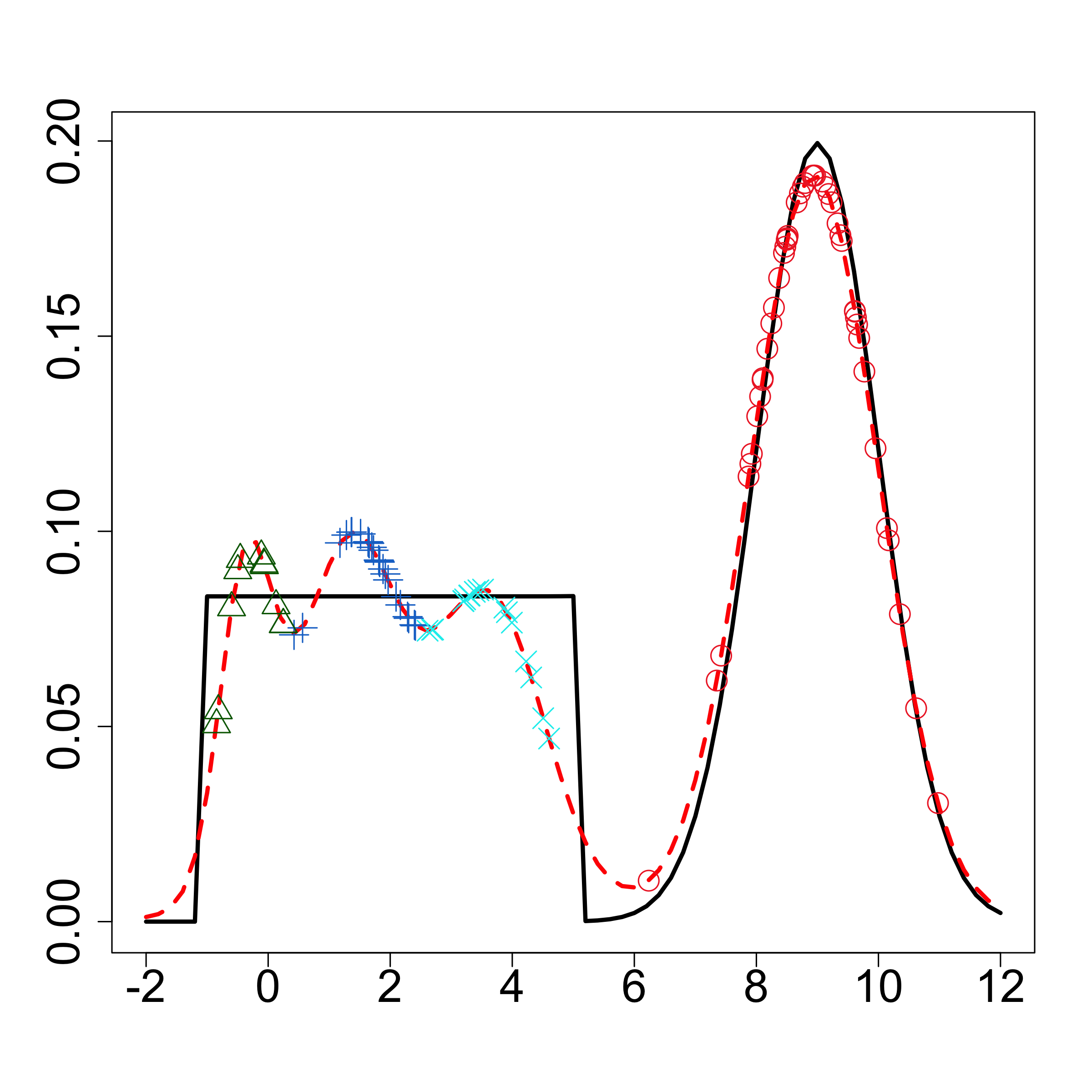
(a) Bayesian Model-Based Clustering Point Estimate

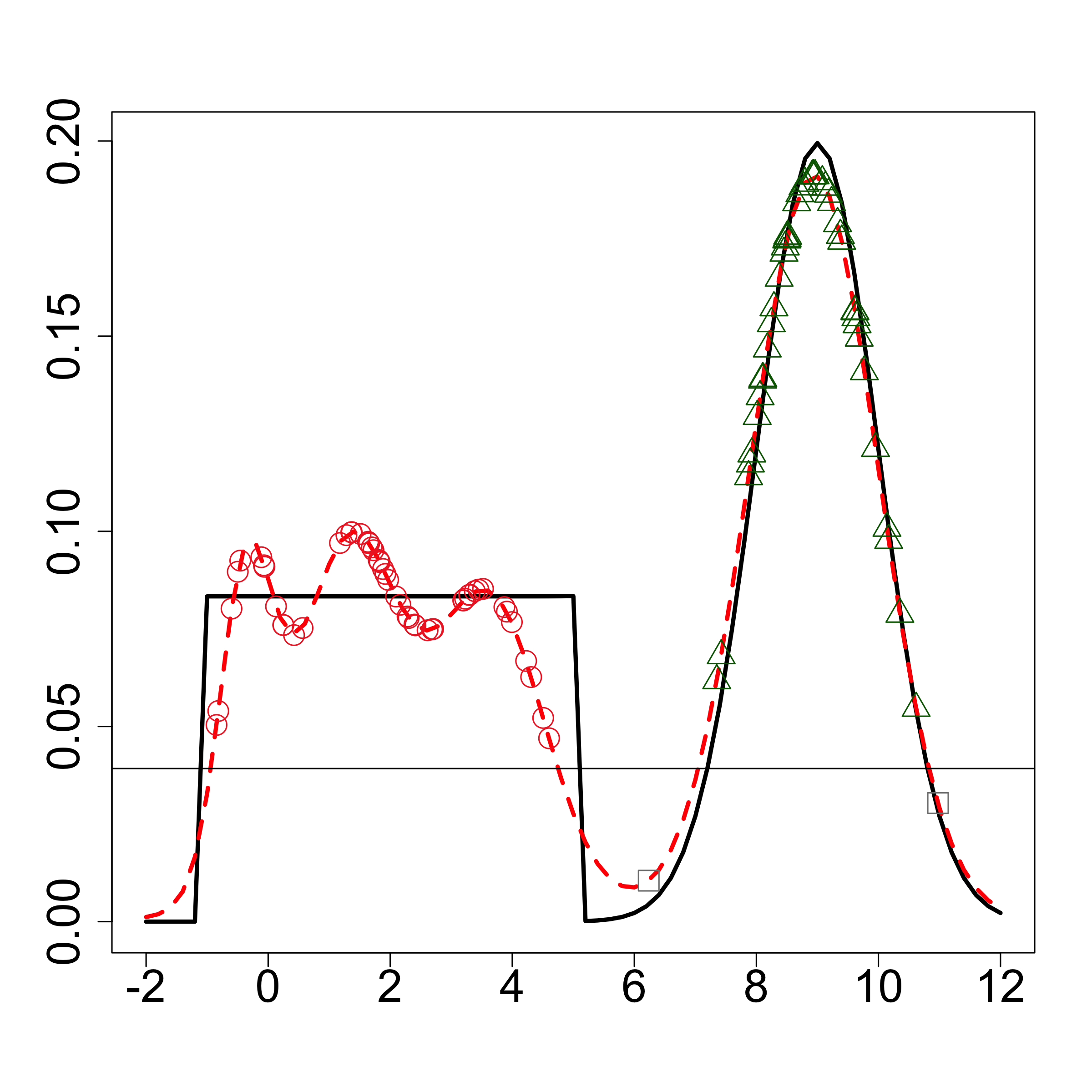
(b) Bayesian Level-Set Clustering Point Estimate

Figure 1: We see the cluster splitting phenomenon among the clusters obtained (left) by fitting a Dirichlet process mixture of Gaussian distributions and finding the partition that minimizes expected VI loss under the posterior. Our Bayesian level-set clustering point estimate (right) does not suffer from this phenomenon, despite the obvious bias in the posterior expectation of the density caused by the poor choice of prior distribution. We display a random subsample of the data in both plots, with their y-coordinates set to the expectation of the density at their locations, and with cluster assignments reflected by the color and shape of the points. The dashed red line is the expected density under the posterior. The solid line shown in black is the true data-generating density.

Rather than avoid Bayesian clustering when the classical mixture approach fails, we propose that Bayesian researchers explore new ways to target meaningful clusters in the data. To accommodate the rich variety of notions of “meaningful clusters” that arise in different applications, we recommend the development of clustering methods that target a population-level clustering given by a suitable function of the sampling density.

Suppose that data are drawn from sample space $\mathcal{X}$, and denote by $\mathscr{D}(\mathcal{X})$ the space of densities on $\mathcal{X}$. Then, letting $\mathscr{P}(\mathcal{X})$ refer to the space of all possible partitions of $\mathcal{X}$, we can define functions $\Psi:\mathscr{D}(\mathcal{X})\to\mathscr{P}(\mathcal{X})$ that map from densities on $\mathcal{X}$ to partitions of $\mathcal{X}$. In the example from Figure 1 (b), $\Psi$ was chosen as the partition of $\mathcal{X}$ corresponding to the $0.04$ level set of the density of the data. Partitions of the sample space determine well-defined clusterings since, for any sample $\mathcal{X}_{n}=\{x_{1},\ldots,x_{n}\}\subseteq\mathcal{X}$, a partition of $\mathcal{X}$ induces a partition on $\mathcal{X}_{n}$. For an illustration, see Figure 1 (b). For a particular $\Psi$ and dataset $\mathcal{X}_{n}$, we will denote maps from densities on $\mathcal{X}$ to the partition on $\mathcal{X}_{n}$ induced by $\Psi$ with the lower case $\psi:\mathscr{D}(\mathcal{X})\to\mathscr{P}(\mathcal{X}_{n})$. Such functions implicitly depend on the sample $\mathcal{X}_{n}$, but we suppress that dependence to simplify notation.

Next, let $D(\psi(f),\bm{C})$ denote a loss for clustering $\bm{C}\in\mathscr{P}(\mathcal{X}_{n})$ relative to the clustering $\psi(f)\in\mathscr{P}(\mathcal{X}_{n})$. If $f_{0}$ is the true data-generating density, then the target clustering is $\bm{C}_{0}=\psi(f_{0})$. In practice $f_{0}$ is unknown, so we represent uncertainty in the unknown density using a Bayesian posterior $f\sim P_{M}(\cdot|\mathcal{X}_{n})$ based on the model $M$. This allows us to define a Bayesian decision-theoretic estimator $\widehat{\psi}_{M}(\mathcal{X}_{n})$, obtained by minimizing the expected posterior loss: $\widehat{\psi}_{M}(\mathcal{X}_{n})=\operatorname*{arg\,min}_{\bm{C}\in\mathscr{P}(\mathcal{X}_{n})}E_{f\sim P_{M}(\cdot|\mathcal{X}_{n})}[D(\psi(f),\bm{C})]$.

There is extensive literature on clustering strategies that can be described as functions of the data-generating density $f$, which we generically call density-based clustering (campello2020density; bhattacharjee2021survey; chacon2015population; menardi2016modal). These methods target a well-defined object at the population level (chacon2015population; menardi2016modal). For instance, $\psi$ might divide the space into the basins of attraction of the modes of $f$ and cluster the observations accordingly (chen2016comprehensive; jiang2017modal; arias2016estimation; arias2023unifying; jiang2017consistency; jang2021meanshift++). However, in this article, we will focus on summarizing $f$ by partitioning the observations into connected components of level sets (cuevas2000estimating; sriperumbudur2012consistency; jiang2017density; jang2019dbscan).

Level-set clustering groups data points that fall in the same high density region, while allowing these regions to have complex and potentially non-convex shapes. This situation arises, for example, in the analysis of RNA-sequencing data (jiang2016giniclust; kiselev2019challenges); see Figure 2 for a t-SNE embedding (van2008visualizing) of a dataset that appears to warrant a level-set clustering approach. Level-set clustering tends to be robust to errors in density estimation (jiang2019robustness). See Figure 1 (b) for an illustration, where the posterior expectation of the density under a Dirichlet process mixture of Gaussians exhibits clear bias relative to the true density but level-set clustering point estimate $\widehat{\psi}_{M}(\mathcal{X}_{n})$ still captures the natural partition of the observations into high-density regions. Level-set clustering also has the advantage of identifying “noise points” that do not fall in high density regions; see Figure 4 for an example motivated by cosmology.

In this article, we propose the BALLET (BAyesian LeveL seT) clustering methodology which synthesizes the rich literature on Bayesian density estimation (escobar1995bayesian; lavine1992some; muller2015bayesian; ma2017adaptive; chattopadhyay2020nearest), advances in theory and algorithms for computing Bayesian decision-theoretic clustering point estimates (fritsch2009improved; rastelli2018optimal; dahl2022search), methods for interpretable characterization of uncertainty in Bayesian clustering (wade2018bayesian), the established theoretical and applied literature on algorithmic density-based clustering (ester1996density; schubert2017dbscan) and frequentist level-set clustering (sriperumbudur2012consistency; rinaldo2010generalized).

We develop theory supporting our methodology and demonstrate its application to simulated and real data sets, highlighting advantages over traditional model based clustering as well as algorithmic level-set clustering. Since it is developed as a summary of a posterior distribution on the data-generating density $f$, BALLET is agnostic to particular modeling decisions and can be rapidly deployed as a simple add-on to a Bayesian analysis. Along with this article, we provide open source R software to extract BALLET clustering solutions from data $\mathcal{X}_{n}$ and samples $f^{(1)},\dots,f^{(s)}$ from the posterior distribution of $f$. This flexibility has allowed us to exploit the great variety of Bayesian density models whereas traditional Bayesian clustering has been restricted to using mixtures of parametric components as a model for the data density $f$. Throughout this article we will demonstrate the advantage of this versatility by invoking a number of different state-of-the-art Bayesian density estimation models.

The remainder of this article is organized as follows. In Section 2, we introduce notation and carefully describe the BALLET methodology. In Section 3 we present a strategy for interpretable quantification of clustering uncertainty. In Section 4, we show that under mild conditions, the BALLET estimator is asymptotically consistent for estimating the true level-set clusters. Next, we apply the method to several toy challenge datasets for clustering in Section 5 and report the results of a case study analyzing cosmological sky survey data in Section 6. We conclude, discussing results and directions for future work, in Section 7. Additional related work, proofs, and results from our data analyses (like figures and tables prefixed by the letter ‘S’) can be found in the supplementary materials.

2 Bayesian Level-Set Clustering Methodology

We start by expanding on the notational conventions of Section 1. Suppose that our data $\mathcal{X}_{n}=\{x_{1},\ldots,x_{n}\}$ are drawn independently from unknown density $f_{0}\in\mathscr{D}(\mathcal{X})$ on sample space $\mathcal{X}$ (taken to be $\mathbb{R}^{d}$ in much of this article), where $\mathscr{D}(\mathcal{X})$ denotes the space of densities on $\mathcal{X}$ with respect to the Lebesgue measure. Let $S_{\lambda}=\{x\in\mathcal{X}:f_{0}(x)\geq\lambda\}$ denote the $\lambda$ level set of $f_{0}$. If we temporarily use $W_{1},\dots,W_{k*}$ to denote the topologically connected components of $S_{\lambda}$, then the level-set clustering associated with $f_{0}$ will be the collection $\bm{C}=\{C_{1},\dots,C_{k}\}$ of $k\leq k^{*}$ non-empty sets in $\{W_{1}\cap\mathcal{X}_{n},\dots,W_{k^{*}}\cap\mathcal{X}_{n}\}$.

Level set clusterings are sub-partitions, since $C_{i}\cap C_{j}=\emptyset$ for all $i\neq j$ and $\cup_{i=1}^{k}C_{i}\subseteq\mathcal{X}_{n}$ but, unlike regular partitions, the presence of noise points not assigned to any cluster can lead to $\cup_{i=1}^{k}C_{i}\neq\mathcal{X}_{n}$. For a specific sub-partition $\bm{C}$, $A=\cup_{i=1}^{k}C_{i}$ denotes the active or core points, while the remaining unclustered observations $I=\mathcal{X}_{n}\setminus A$ are inactive or noise points. In Figure 1(b) noise points are shown in grey. Every sub-partition of size $k$ is associated with a unique partition of size $k+1$, where the extra set in the partition contains the noise points. However, since this is not a one-to-one association, we explicitly work with the non-standard setup of regarding a clustering as a sub-partition rather than a partition. To this end, we re-purpose the notation $\mathscr{P}(\mathcal{X}_{n})$ to denote the space of all sub-partitions of $\mathcal{X}_{n}$.

2.1 Decision-Theoretic Framework

We will focus on finding the sub-partition of the data $\mathcal{X}_{n}$ associated with the connected components of $S_{\lambda}$. We let $\psi_{\lambda}:\mathscr{D}(\mathcal{X})\mapsto\mathscr{P}(\mathcal{X}_{n})$ be the level-$\lambda$ clustering function, by which we mean that $\psi_{\lambda}(f)$ returns the sub-partition $\bm{C}$ of $\mathcal{X}_{n}$ associated with the level-$\lambda$ connected components of $f$.

To begin a density-based cluster analysis we choose a Bayesian model $M$ for the unknown density $f$. Examples of $M$ include not only kernel mixture models but also Bayesian nonparametric approaches that do not involve a latent clustering structure, such as Polya trees (lavine1992some; wong2010optional; ma2017adaptive) and logistic Gaussian processes (lenk1991towards; tokdar2007towards; riihimaki2014laplace). Under $M$, we obtain a posterior distribution $P_{M}(f|\mathcal{X}_{n})$ for the unknown density of the data. This also induces a posterior on the $\lambda$ level set of $f$. Based on this posterior, we define $\widehat{\psi}_{\lambda,M}$ as an estimator of $\psi_{\lambda}(f_{0})$.

Let $D(\psi_{\lambda}(f),\bm{C})$ denote a loss function measuring the quality of sub-partition $\bm{C}$ relative to the ground-truth $\psi_{\lambda}(f)$. The Bayes estimator of the sub-partition then corresponds to the value that minimizes the expectation of the loss under the posterior of $f$:

$$\widehat{\psi}_{\lambda,M}(\mathcal{X}_{n})=\operatorname*{arg\,min}_{\bm{C}\in\mathscr{P}(\mathcal{X}_{n})}E_{f\sim P_{M}(\cdot|\mathcal{X}_{n})}[D(\psi_{\lambda}(f),\bm{C})].$$ (1)

In practice, we use a Monte Carlo approximation based on samples $f^{(1)},\dots,f^{(S)}$ from $P_{M}(f|\mathcal{X}_{n})$: $\widehat{\psi}_{\lambda,M}(\mathcal{X}_{n})\approx\operatorname*{arg\,min}_{\bm{C}\in\mathscr{P}(\mathcal{X}_{n})}\sum_{s=1}^{S}D(\psi_{\lambda}(f^{(s)}),\bm{C})$.

Three major roadblocks stand in the way of calculating this estimator. First, evaluating $\psi_{\lambda}(f^{(s)})$ is problematic as identifying connected components of level sets of $f^{(s)}$ is extremely costly if the data lie in even a moderately high-dimensional space. Instead, we will use a surrogate clustering function $\widetilde{\psi}_{\lambda}$, which approximates the true clustering function and is more tractable. We will discuss this further in Sections 2.2 and 2.3.

The second roadblock is the fact that we must design an appropriate loss function $D$ for use in estimating level set clusterings. Since these objects are sub-partitions, usual loss functions on partitions that are employed in model-based clustering will be inappropriate. We will discuss the issue further and introduce an appropriate loss in Section 2.4.

Finally, optimizing the risk function over the space of all sub-partitions, as shown in equation (1), will be computationally intractable, since the number of elements in $\mathscr{P}(\mathcal{X}_{n})$ is immense. However, leveraging on the usual Bayesian clustering literature, we could adapt the discrete optimization algorithm of dahl2022search to handle our case of sub-partitions.

Having addressed these issues, we refer to the resulting class $\{\widehat{\psi}_{\lambda,M}\}$ as BALLET estimators. In Section 4 we show that, despite our modifications to the standard Bayesian decision-theoretic machinery of equation (1), under suitable models $M$ for the density $f$, the BALLET estimator $\widehat{\psi}_{\lambda,M}$ consistently estimates the level-$\lambda$ clustering based on $f_{0}$.

2.2 Surrogate Clustering Function

Computing the clustering function $\psi_{\lambda}(f)$ based on the level set $S_{\lambda,f}=\{x\in\mathcal{X}:f(x)\geq\lambda\}$ involves two steps. The first is to identify the subset of observations $A_{\lambda,f}=S_{\lambda,f}\cap\mathcal{X}_{n}$, called the active points for $f$, and the second is to separate the active points according to the (topologically) connected components of $S_{\lambda,f}$. The first step is no more difficult than evaluating $f$ at each of the $n$ observations and checking whether $f(x_{i})\geq\lambda$ for each $i\in\{1,\dots,n\}$. However, identifying the connected components of $S_{\lambda,f}$ can be computationally intractable unless $\mathcal{X}$ is one dimensional. This is a familiar challenge in the algorithmic level set clustering literature (campello2020density).

A common approach with theoretical support (sriperumbudur2012consistency) is to approximate the level set $S_{\lambda,f}$ with a tube of diameter $\delta>0$ around the active points: $T_{\delta}(A)=\cup_{x_{i}\in A}B(x_{i},\delta/2)$, where $B(x,\delta/2)$ is the open ball of radius $\delta/2$ around $x$ and $A=A_{\lambda,f}$ denotes the active points. Computing the connected components of $T_{\delta}(A)$ is straightforward. If we define $G_{\delta}(A)$ as the $\delta$-neighborhood graph with vertices $A$ and edges $\{(x,x^{\prime})\in A\times A\;|\,\|x-x^{\prime}\|<\delta\}$, then two points $x,x^{\prime}\in\mathcal{X}$ lie in the same connected component of $T_{\delta}(A)$ if and only if there exist active points $x_{i},x_{j}\in A$ such that $\|x-x_{i}\|<\frac{\delta}{2}$, $\|x^{\prime}-x_{j}\|<\frac{\delta}{2}$ and $x_{i}$, $x_{j}$ are connected by a path in $G_{\delta}(A)$. The problem simplifies further since we only need to focus on the active points: any $x_{i},x_{j}\in A$ lie in the same connected component of $T_{\delta}(A)$ if and only if $x_{i},x_{j}$ are connected by a path in $G_{\delta}(A)$.

Hence, we define a computationally-tractable surrogate clustering function

$$\widetilde{\psi}_{\delta,\lambda}(f)=\texttt{CC}(G_{\delta}(A_{\lambda,f}))$$ (2)

where the dependence on the density $f$ and level $\lambda$ enter through the active points $A_{\lambda,f}=\{x\in\mathcal{X}_{n}|f(x)\geq\lambda\}$, and CC is the function that maps graphs to the graph-theoretic connected components of their vertices (see e.g. sanjoy2008algorithms).

The above procedure is equivalent to applying single-linkage clustering to the active points $A_{\lambda,f}$, with the hierarchical clustering tree cut at level $\delta$. Since the (optimal) time complexity and space complexity achieved by efficient single-linkage clustering algorithms are $O(n^{2})$ and $O(n)$, respectively (sibson1973slink), we can see that the computational complexity of evaluating our surrogate clustering function $\widetilde{\psi}_{\delta,\lambda}(f)$ is $O(n\kappa+n^{2})$ and the space complexity is $O(n)$, where $\kappa$ is the cost of evaluating the density $f$ at a single observation.

We now discuss the elicitation of the loss parameters $\lambda,\delta>0$ that we have introduced.

2.3 Choosing the BALLET loss parameters $\lambda$ and $\delta$

Some theoretical (jiang2017density; steinwart2015fullyAdaptive) and practical (cuevas2000estimating; ester1996density; schubert2017dbscan) strategies for choosing the loss parameters $\lambda$ and $\delta$ have previously been discussed in the level set clustering literature. Below we comment on some strategies we used in choosing the loss parameters, which build on this literature.

The loss parameter $\lambda$ influences the decision theoretic analysis in (1) by targeting different level set clusters, depending on the goals of the analyst. Instead of eliciting $\lambda$ directly, it is often more intuitive to choose an approximate proportion of noise points $\nu$. To choose a $\lambda$ corresponding to the chosen $\nu\in(0,1)$, we use $\lambda_{\nu}=q_{\nu}(\{\hat{f}(x_{i}):x_{i}\in\mathcal{X}_{n}\})$ where $\hat{f}(x)=\operatorname{Median}_{f\sim P_{M}(\cdot|\mathcal{X}_{n})}[f(x)]$ is the posterior median density value and $q_{\nu}$ is the quantile function. We illustrate different strategies for choosing $\nu$ later in the paper. The issue of sensitivity to the exact choice of this parameter is briefly discussed in Section 7.

To guide our choice of $\delta$, given the fraction of noise points $\nu\in(0,1)$ and a fixed number $k\in\mathbb{N}$, one may note (see e.g.  jiang2017density) that the popular clustering method DBSCAN (ester1996density) is a special case of (2) when $f=f_{k}$ is the $k$-nearest neighbor density estimator, $\lambda=q_{\nu}(\{f_{k}(x_{i}):x_{i}\in\mathcal{X}_{n}\})$ and $\delta=\max\left(\{\delta_{k}(x_{i}):f_{k}(x_{i})\geq\lambda,x_{i}\in\mathcal{X}_{n}\right\})$, where $\delta_{k}(x)$ is the distance of point $x$ to its $k$th nearest-neighbor in $\mathcal{X}_{n}$. We adapt this heuristic to our setup, choosing $\delta=q_{.99}\left(\{\delta_{k}(x_{i}):\hat{f}(x_{i})\geq\lambda\}\right)$ where $\hat{f}$ is the posterior median density.

Our choice of $\delta$ ensures that balls of radius $\delta$ around almost all (99%) of the core points contain at least $k$ observations. This may be compared with the theoretical condition in Supplementary Material S3 (e.g. see Lemma S2 and its proof) that requires the $\delta$ to be large enough to ensure that each such ball contains at least one observation. We fix the default value of $k=\lfloor\log_{2}(n)\rfloor$ for all of our analyses.

2.4 Loss Function for Comparing Sub-partitions

There is an expansive literature on loss functions for estimating partitions (e.g., binder1978bayesian; meila2007comparing; vinh2009information), and many of these articles establish compelling theoretical properties motivating their use. Unfortunately, we cannot directly use these losses for sub-partitions. While each sub-partition $\bm{C}=\{C_{1},\ldots,C_{k}\}$ of the data $\mathcal{X}_{n}$ can be associated with a regular partition $\bm{C}\cup I$ of $\mathcal{X}_{n}$ by considering the noise points $I=\mathcal{X}_{n}\setminus(\cup_{h=1}^{k}C_{h})$ as a separate cluster, this is a many-to-one mapping that looses information about the identity of the noise cluster. To see why this can be problematic, for some $C\subseteq\mathcal{X}_{n}$ consider two sub-partitions $\bm{C}=\{C\}$ and $\bm{C}^{\prime}=\{\mathcal{X}_{n}\setminus C\}$ that have a single cluster with noise points given by $I=\mathcal{X}_{n}\setminus C$ and $I^{\prime}=C$ respectively. Intuitively, the level set clustering $\bm{C}$ and $\bm{C}^{\prime}$ are incredibly different, but any loss function on partitions will assign $L(\{C,I\},\{C^{\prime},I^{\prime}\})=0$ if the identity of the noise cluster is ignored.

Hence, we propose a new loss that modifies the popular Binder’s loss (binder1978bayesian) to be appropriate for the sub-partitions encountered in level set clustering. This loss, called Inactive/Active Binder’s Loss or IA-Binder’s loss for brevity, is a combination of Binder’s loss restricted to data points that are active in both partitions along with a penalty for points which are active in one partition and inactive in the other. To formally define IA-Binder’s loss, we will represent any sub-partition $\bm{C}=\{C_{1},\ldots,C_{k}\}\in\mathscr{P}(\mathcal{X}_{n})$ with a length $n$ allocation vector $\bm{c}=(c_{1},\ldots,c_{n})\in\{0,1\ldots,k\}^{n}$ such that $c_{i}=h$ if $x_{i}\in C_{h}$ and $c_{i}=0$ if $x_{i}\in\mathcal{X}_{n}\setminus\cup_{h=1}^{k}C_{h}$. Given two partitions $\bm{C},\bm{C}^{\prime}$ with active sets $A,A^{\prime}\subseteq\mathcal{X}_{n}$ and allocation vectors $\bm{c},\bm{c}^{\prime}$, the loss between them is defined as

$$L_{\text{IA-Binder}}(\bm{C},\bm{C}^{\prime})$$

$$=(n-1)\big{(}m_{ai}\left|A\cap I^{\prime}\right|+m_{ia}\left|I\cap A^{\prime}\right|\big{)}+\sum_{\begin{subarray}{c}1\leq i<j\leq n\\ x_{i},x_{j}\in A\cap A^{\prime}\end{subarray}}a\mathds{1}_{\left[c_{i}=c_{j};c^{\prime}_{i}\neq c^{\prime}_{j}\right]}+b\mathds{1}_{\left[c_{i}\neq c_{j};c^{\prime}_{i}=c^{\prime}_{j}\right]},$$ (3)

where $I=\mathcal{X}_{n}\setminus A$ and $I^{\prime}=\mathcal{X}_{n}\setminus A^{\prime}$ denote the inactive sets of $\bm{C}$ and $\bm{C}^{\prime}$. The summation term in section 2.4 is Binder’s loss with parameters $a,b>0$ restricted to points that are active in both the sub-partitions. The first two terms, based on parameters $m_{ai},m_{ia}>0$, correspond to a loss of $(n-1)m_{ai}$ and $(n-1)m_{ia}$ incurred by points which are active in $\bm{C}$ but inactive in $\bm{C}^{\prime}$ and vice versa. In this paper, we will mainly focus on the choice of $a=b$ and $m_{ai}=m_{ai}=m\geq a/2$. Under these conditions, the proof of Lemma 1 shows that $L_{\text{IA-Binder}}$ satisfies metric properties on $\mathscr{P}(\mathcal{X}_{n})$.

Given any distribution on $\bm{C}$, we can compute the Bayes risk for an estimate $\bm{C}^{\prime}$ as the posterior expectation of the IA-Binder’s loss:

$$R_{\text{IA-Binder}}(\bm{C}^{\prime})= E[L_{\text{IA-Binder}}(\bm{C},\bm{C}^{\prime})]$$

$$= (n-1)\big{(}m_{ai}\sum_{i=1}^{n}\Pr(x_{i}\in A)\mathds{1}_{\left[x_{i}\in I^{\prime}\right]}+m_{ia}\sum_{i=1}^{n}\Pr(x_{i}\in I)\mathds{1}_{\left[x_{i}\in A^{\prime}\right]}\big{)}\quad+$$

$$\quad\quad\sum_{1\leq i<j\leq n}\mathds{1}_{\left[x_{i}\in A^{\prime},x_{j}\in A^{\prime}\right]}\big{(}a\Pr(x_{i}\in A,x_{j}\in A,c_{i}=c_{j})\mathds{1}_{\left[c^{\prime}_{i}\neq c^{\prime}_{j}\right]}\quad+$$

$$\quad\quad\quad\quad\quad\quad\quad b\Pr(x_{i}\in A,x_{j}\in A,c_{i}\neq c_{j})\mathds{1}_{\left[c^{\prime}_{i}=c^{\prime}_{j}\right]}\big{)}.$$ (4)

The probabilities are computed based on the random clustering $\bm{C}$; particularly, $\bm{c}=(c_{1},\ldots,c_{n})$ denotes the allocation vector of $\bm{C}$, and $A$ and $I$ denote its active and inactive points. Here we will use $\bm{C}=\widetilde{\psi}_{\delta,\lambda}(f)$, where $f$ is drawn from the posterior $P_{M}(\cdot|\mathcal{X}_{n})$.

Putting it all together, we have our BALLET estimator for level-$\lambda$ clustering:

$$\widehat{\psi}_{\delta,\lambda,M}(\mathcal{X}_{n}) =\operatorname*{arg\,min}_{\bm{C}^{\prime}\in\mathscr{P}(\mathcal{X}_{n})}E_{f\sim P_{M}(\cdot|\mathcal{X}_{n})}[L_{\text{IA-Binder}}(\widetilde{\psi}_{\delta,\lambda}(f),\bm{C}^{\prime})]$$ (5)

$$\approx\operatorname*{arg\,min}_{\bm{C}^{\prime}\in\mathscr{P}(\mathcal{X}_{n})}\sum_{s=1}^{S}L_{\text{IA-Binder}}(\widetilde{\psi}_{\delta,\lambda}(f^{(s)}),\bm{C}^{\prime})$$

where the dependence of the estimator on the data is mediated by the posterior distribution $P_{M}(\cdot|\mathcal{X}_{n})$ from which we generate samples $f^{(1)},\dots,f^{(S)}$.

We can pre-compute Monte Carlo estimates of the probabilities appearing in equation (2.4). Then, obtaining our BALLET estimate is just a matter of optimizing the objective function. For the examples in this article, and in the open-source software which accompanies it, we searched the space of sub-partitions using a modified implementation of the SALSO algorithm proposed by dahl2022search. In general, algorithms to optimize an objective function over the space of partitions (e.g., fritsch2009improved; rastelli2018optimal) can be adapted to search the space of sub-partitions by introducing a means to distinguish the set of inactive points. Since the algorithms typically operate on allocation vector representations of partitions, we accomplished this by adopting the convention that the integer label $(0)$ is reserved for observations in the noise set.

3 Credible Bounds

Once we have obtained a point estimate for our level-$\lambda$ clustering $\psi_{\lambda}(f_{0})$, we would like to characterize our uncertainty in the estimate. One popular strategy in clustering analyses is to examine the $n\times n$ posterior similarity matrix, whose $i,j$th entry contains the posterior co-clustering probability $\Pr(c_{i}=c_{j}|\mathcal{X}_{n})$. If all the entries in this matrix are nearly $0$ or $1$, we can conclude there is less uncertainty about the clustering structure than if all entries in the matrix hover between those extremes. However, it is not easy to extract further information by examining this matrix. Our sub-partition setting also introduces additional complications since the status of each pair of points can be in four possible states: (i) both points are active and co-clustered, (ii) both points are active but in separate clusters, (iii) one point is active while the other is inactive, (iv) both points are inactive.

An appealing alternative is to adapt the method proposed in wade2018bayesian to compute credible balls for level-set partitions. To find a credible ball around the point estimate $\widehat{\bm{C}}$ with credible level $1-\alpha$ for $\alpha\in[0,1]$, we first find

$$\epsilon^{*}=\operatorname*{arg\,min}_{\epsilon>0}\Pr(\widetilde{\psi}_{\delta,\lambda}(f)\in B_{\epsilon}(\widehat{\bm{C}})|\mathcal{X}_{n})\geq 1-\alpha,$$ (6)

where the probability is computed under $f\sim P_{M}(\cdot|\mathcal{X}_{n})$ sampled from the posterior distribution and $B_{\epsilon}(\bm{C})=\{\bm{C}^{\prime}\in\mathscr{P}(\mathcal{X}_{n}):L_{\text{IA-Binder}}(\bm{C},\bm{C}^{\prime})\leq\epsilon\}$ is the ball of radius $\epsilon$ around $\bm{C}$. Then, the posterior distribution will assign a probability close to $1-\alpha$ to the event that $B_{\epsilon^{*}}(\widehat{\bm{C}})$ contains $\bm{C}=\widetilde{\psi}_{\delta,\lambda}(f)$, the unknown level set sub-partition.

The $1-\alpha$ coverage credible ball $B_{\epsilon^{*}}(\widehat{\bm{C}})$ typically contains a large number of possible sub-partitions. To summarize credible balls in the space of data partitions, wade2018bayesian recommend identifying vertical and horizontal bounds based on the partial ordering of partitions associated with a Hasse diagram. The vertical upper bounds were defined as the partitions in $B_{\epsilon^{*}}(\widehat{\bm{C}})$ that contained the smallest number of sets; vertical lower bounds, accordingly, were the partitions in $B_{\epsilon^{*}}(\widehat{\bm{C}})$ that contained the largest number of sets; horizontal bounds were those partitions in $B_{\epsilon^{*}}(\widehat{\bm{C}})$ which were the farthest from $\widehat{\bm{C}}$ in the distance $L_{\text{IA-Binder}}$.

In our setting, in addition to similarity of sub-partitions in terms of their clustering structure, we must also compare inclusion or exclusion of observations from the active set. Uncertainty in the clustering structure will be partly attributable to uncertainty in which points are active. Fortunately, the space of sub-partitions is also a lattice with its associated Hasse diagram (Supplementary Material S2). We can move down the sub-partition lattice by splitting clusters or removing items from the active set, while we can move up the lattice of sub-partitions by merging clusters or absorbing noise points into the active set.

We propose the following computationally efficient algorithm for computing upper and lower bounds for the credible ball. Suppose we know our credible ball radius $\epsilon^{*}$ from Equation 6 needed to achieve the desired coverage. We seek our upper bound by starting at the point estimate and greedily adding to the active set, one at a time, the item from the inactive set that has the greatest posterior probability of being active and re-examining the resulting connected components; this continues until we find a sub-partition that is farther than $\epsilon^{*}$ from the point estimate. To find a lower bound we perform the analogous greedy removal process. The resulting bounds from applying this algorithm can be seen in Figures 3, S10 and 5.

4 Consistency of Bayesian Density-based Clustering

In this section, we show large sample consistency of a generic Bayesian density-based clustering estimator of the form

$$\widehat{\psi}_{M}(\mathcal{X}_{n}) =\operatorname*{arg\,min}_{\bm{C}\in\mathscr{P}(\mathcal{X}_{n})}E_{f\sim P_{M}(\cdot|\mathcal{X}_{n})}[D(\widetilde{\psi}(f),\bm{C})],$$ (7)

where $D$ is a loss on the space $\mathscr{P}(\mathcal{X}_{n})$ of data sub-partitions and $\widetilde{\psi}:\mathscr{D}(\mathcal{X})\to\mathscr{P}(\mathcal{X}_{n})$ is an easy-to-compute surrogate that approximates the target density-based clustering function $\psi:\mathscr{D}(\mathcal{X})\to\mathscr{P}(\mathcal{X}_{n})$. Similar to previous sections, we omit notation for the implicit dependence of $D$, $\widetilde{\psi}$, and $\psi$ on $\mathcal{X}_{n}$. We will assume that the loss $D$ is a metric that takes values in $[0,1]$. We state our consistency result in terms of convergence in probability. Recall that a sequence of random variables $\{X_{n}\}_{n\geq 1}$ converges to zero in probability, denoted by $X_{n}\overset{P}{\to}0$ as $n\to\infty$, if $\lim_{n\to\infty}P(|X_{n}|>\epsilon)=0$ for every $\epsilon>0$.

Under some assumptions to be stated later (Section 4.1), the following theorem establishes consistency of the estimator (7). In particular, when the data $\mathcal{X}_{n}$ are generated i.i.d. from $f_{0}$, it states that the Bayesian density-based clustering estimator defined in (7) will be close to the target clustering $\psi(f_{0})$ in terms of the loss $D$ for large values of $n$.

Theorem 1.

(Consistency of Density-based clustering) Suppose that Assumptions 1, 2 and 3 in Section 4.1 hold, and $\mathcal{X}_{n}=\{x_{1},\ldots,x_{n}\}\overset{i.i.d.}{\sim}f_{0}$. Then

$$0\leq D(\widehat{\psi}_{M}(\mathcal{X}_{n}),\psi(f_{0}))\leq 2\delta_{1}(\mathcal{X}_{n})+2\delta_{2}(\mathcal{X}_{n})\overset{P}{\to}0\qquad\text{as $n\to\infty$,}$$

where $\widehat{\psi}_{M}(\mathcal{X}_{n})$ is the density-based clustering (7) and the error terms $\delta_{1}$ and $\delta_{2}$ are as defined in Assumptions 2 and 3.

In Section 4.2, we establish the validity of Assumptions 1, 2 and 3 specifically for the BALLET estimator $\widehat{\psi}_{\delta,\lambda,M}(\mathcal{X}_{n})$ that was introduced in (5). Notably, $\widehat{\psi}_{\delta,\lambda,M}(\mathcal{X}_{n})$ represents a special case of (7), where $\widetilde{\psi}=\widetilde{\psi}_{\delta,\lambda}$ is the surrogate clustering function defined in (2), $\psi=\psi_{\lambda}$ is the level-$\lambda$ clustering function defined in Section 2.1, and $D=\binom{n}{2}^{-1}L_{\text{IA-Binder}}$ is a re-scaled version of the Inactive-Active Binder’s loss (2.4). For large values of $n$, the theorem shows that with high-probability the estimated BALLET clustering will be close (in the metric $D$) to the true level set clustering $\psi_{\lambda}(f_{0})$.

We now discuss the assumptions underlying the above theorem (Section 4.1) and verify them for BALLET estimators (Section 4.2). All the proofs in this section (including that of Theorem 1) are provided in Supplementary Material S3.

4.1 Assumptions of Theorem 1

Assumption 1.

Suppose that $D:\mathscr{P}(\mathcal{X}_{n})\times\mathscr{P}(\mathcal{X}_{n})\to[0,1]$ is a metric.

As stated earlier, we assume that the loss $D$ is a metric bounded above by one. While we can enforce this boundedness by suitably re-scaling $D$ or replacing it by $\min(D,1)$, the metric properties of $D$, particularly non-negativity, symmetry, and triangle inequality, are crucially used in the proof of Theorem 1.

Next, we assume that the Bayesian model $M$ for the unknown density $f$ is such that its posterior distribution $P_{M}(\cdot|\mathcal{X}_{n})$ on densities, under samples $\mathcal{X}_{n}=\{x_{1},\ldots,x_{n}\}\overset{i.i.d.}{\sim}f_{0}$, contracts at rate $\{\epsilon_{n}\}$ in the $L_{\infty}$ metric to $f_{0}$. More precisely, given the $L_{\infty}$ metric $\|f-g\|_{\infty}\doteq\sup_{x\in\mathcal{X}}|f(x)-g(x)|$, we make the assumption that:

Assumption 2 (Posterior contraction in $L_{\infty}$).

If $\mathcal{X}_{n}=\{x_{1},\ldots,x_{n}\}\overset{i.i.d.}{\sim}f_{0}$, then there is a non-random sequence $\{\epsilon_{n}\}_{n\geq 1}\subseteq\mathbb{R}_{+}$ such that

$$\delta_{1}(\mathcal{X}_{n})\doteq P_{M}\left(f:\|f-f_{0}\|_{\infty}\geq\epsilon_{n}K_{n}\big{|}\mathcal{X}_{n}\right)\overset{P}{\to}0$$

as $n\to\infty$, for every sequence $\{K_{n}\}_{n\in\mathbb{N}}\subseteq\mathbb{R}$ such that $\lim_{n\to\infty}K_{n}=\infty$.

Establishing posterior contraction in the $L_{\infty}$ metric, as required in Assumption 2, constitutes an active area of research in Bayesian non-parametrics. For the case of univariate density estimation on $\mathcal{X}=[0,1]$, such contraction rates were initially established for kernel mixture models, random histogram priors based on dyadic partitions, and Gaussian process and wavelet series priors on the log density (gine2011rates; castillo2014bayesian). Recent work for $\mathcal{X}=[0,1]$ has shown a minimax optimal contraction rate of $\epsilon_{n}=\left(\frac{\log n}{n}\right)^{\frac{\alpha}{2\alpha+1}}$ based on Pólya trees (castillo2017polya; castillo2021spike) and wavelet series priors on the log-density (naulet2022adaptive), where $\alpha\in(0,1]$ is the apriori unknown Hölder smoothness of $f_{0}$. For the case of multivariate density estimation on $\mathcal{X}=[0,1]^{d}$, contraction rates of the order $\epsilon_{n}=\left(\frac{\log n}{n}\right)^{\frac{\alpha-d/2+\alpha/(\alpha+1)}{2\alpha+d}}$ can be found in li2021posterior and references therein.

Finally, in Assumption 3 we require the distance between the surrogate clustering $\widetilde{\psi}(f)$ and the true clustering $\psi(f_{0})$ to be small in the metric $D$ as long as $f$ is suitably close to $f_{0}$ in the $L_{\infty}$ metric. Intuitively, this requires that (a) $\widetilde{\psi}$ is an accurate surrogate for $\psi$, and (b) $\psi$ is continuous at $f_{0}$ with respect to the $L_{\infty}$ metric.

Assumption 3.

Suppose that $\delta_{2}(\mathcal{X}_{n})\doteq\sup_{f\in\mathscr{D}(\mathcal{X}):\|f-f_{0}\|_{\infty}\leq K_{n}\epsilon_{n}}D(\widetilde{\psi}(f),\psi(f_{0}))\overset{P}{\to}0$ as $n\to\infty$ for some sequence $K_{n}\to\infty$.

Note that we need a common sequence $\{(\epsilon_{n},K_{n})\}_{n\geq 1}$ such that both Assumptions 3 and 2 hold. The use of the $L_{\infty}$ metric in Assumptions 3 and 2 is not important, and the proof of Theorem 1 will remain unchanged if the $L_{\infty}$ metric is replaced by some other metric on $\mathscr{D}(\mathcal{X})$. However, our choice of the $L_{\infty}$ metric is important to verify Assumption 3 for BALLET estimators in Section 4.2.

4.2 Verifying Assumptions for BALLET Estimator

Our BALLET estimator $\widehat{\psi}_{\delta,\lambda,M}(\mathcal{X}_{n})$ from (5) is a special case of (7) when $\widetilde{\psi}=\widetilde{\psi}_{\delta,\lambda}$ is the clustering surrogate function (2) to the level-$\lambda$ clustering function $\psi=\psi_{\lambda}$ defined in Section 2.1, and $D=\binom{n}{2}^{-1}L_{\text{IA-Binder}}$ is a re-scaled version of the Inactive-Active Binder’s loss (2.4). We verify Assumptions 3 and 1 for this setup. The following lemma shows that Assumption 1 is satisfied for suitable choices of constants in loss (2.4).

Lemma 1.

Suppose $0<a=b\leq 1$, $m=m_{ia}=m_{ai}\leq 1$, and $a\leq 2m$. Then $D=\binom{n}{2}^{-1}L_{\text{IA-Binder}}$ is a metric on $\mathscr{P}(\mathcal{X}_{n})$ that is bounded above by 1.

We now verify Assumption 3 in this setup for some mild conditions on the density $f_{0}$ stated in Supplementary Material S3. We roughly require that $f_{0}:\mathbb{R}^{d}\to[0,\infty)$ is continuous and vanishing in the tails (Assumption S4), is not flat around the level $\lambda$ (Assumption S5), and has a level-$\lambda$ clustering that is stable with respect to small perturbations in $\lambda$ (Assumption S6). The condition $\delta_{n}\geq r_{n,\lambda,d}$ in the lemma is used to ensure that the tube-based estimator $T_{\delta_{n}}(A_{f,\lambda})$ from Section 2.2 is a consistent estimator for $S_{\lambda}$.

Lemma 2.

Suppose $\mathcal{X}=\mathbb{R}^{d}$ and the density $f_{0}$ satisfies Assumptions S4, S5 and S6 and is $\alpha$-Hölder smooth for some $\alpha\in(0,1]$. Let $\mathcal{X}_{n}=\{x_{1},\ldots,x_{n}\}\overset{i.i.d.}{\sim}f_{0}$, $D$ be the re-scaled loss from Lemma 1, and $\{\delta_{n}\}_{n\geq 1}$ be any sequence converging to zero such that $\delta_{n}\geq r_{n,\lambda,d}$, where $r_{n,\lambda,d}=C_{1}\left(\frac{\Gamma(d/2+1)d\ln n}{n\lambda}\right)^{1/d}$, $\lambda>0$ is the chosen level, $\Gamma$ denotes the gamma function, and $C_{1}\geq 1$ is a universal constant. Then for any sequence $\{(K_{n},\epsilon_{n})\}_{n\geq 1}\subseteq\mathbb{R}^{2}_{+}$ such that $K_{n}\epsilon_{n}\to 0$, Assumption 3 is satisfied for the BALLET estimator with $\widetilde{\psi}=\widetilde{\psi}_{\delta_{n},\lambda}$ and $\psi=\psi_{\lambda}$. In particular,

$$\delta_{2}(\mathcal{X}_{n})=\sup_{f:\|f-f_{0}\|_{\infty}\leq K_{n}\epsilon_{n}}D(\widetilde{\psi}_{\delta_{n},\lambda}(f),\psi_{\lambda}(f_{0}))\leq C_{0}\left(\max(K_{n}\epsilon_{n},\delta_{n}^{\alpha})+\sqrt{\frac{\ln n}{n}}\right)$$

with probability at least $1-\frac{2}{n}$ when $n\geq n_{0}$. Here $C_{0},n_{0}>0$ are finite constants that may depend on $f_{0}$ and the sequences $\{(\delta_{n},K_{n},\epsilon_{n})\}_{n\geq 1}$ but are independent of $n$ and data $\mathcal{X}_{n}$.

Hence, if the density model $M$ satisfies posterior contraction in the $L^{\infty}$ metric (Assumption 2) for some sequence $\epsilon_{n}\to 0$, the true density $f_{0}$ and level $\lambda>0$ satisfy Assumptions S4, S5 and S6, and the tuning parameter $\delta=\delta_{n}$ (see Section 2.2) is chosen to converge to zero at a rate slower than $\left(\frac{\ln n}{n}\right)^{1/d}$, then Theorem 1 states that

$$\binom{n}{2}^{-1}L_{\text{IA-Binder}}(\widehat{\psi}_{\delta_{n},\lambda,M}(\mathcal{X}_{n}),\psi_{\lambda}(f_{0}))\overset{P}{\to}0\qquad\text{as }n\to\infty,$$ (8)

whenever $\mathcal{X}_{n}=\{x_{1},\ldots,x_{n}\}\overset{i.i.d.}{\sim}f_{0}$ and the loss $L_{\text{IA-Binder}}$ satisfies conditions of Lemma 1.

From the sum-based representation of $L_{\text{IA-Binder}}$ in eq. S1, we note that the convergence in Equation 8 implies that only a vanishingly small fraction of pairs of points from $\mathcal{X}_{n}$ can be clustered differently between $\widehat{\psi}_{\delta_{n},\lambda,M}(\mathcal{X}_{n})$ and $\psi_{\lambda}(f_{0})$ as $n\to\infty$.

5 Illustrative Challenge Datasets

Here we apply our method to three toy challenge datasets. The first two, ‘two moons’ and ‘noisy circles’, are simulated with $N=1000$ observations each. The third dataset is a t-SNE embedding of single cell RNA sequencing data found in an online tutorial (https://www.reneshbedre.com/blog/tsne.html), and includes $N=4406$ observations. All three datasets are visualized in Figure S2.

We first fit the three datasets with a Dirichlet process mixture with a multivariate normal-inverse Wishart base measure. This is frequently invoked as a Bayesian clustering model, and the unknown allocation vector encodes a partition of the data. In addition, we obtain samples $f^{(1)},\dots,f^{(S)}$ from the posterior of $f$ that we will use in BALLET. In this way, fitting only one model to each dataset, we can obtain both “model-based” and “density-level-set” clustering, affording a direct comparison. We visualize the results in Figure 2 where we notice, as expected, that model-based clusters fracture the data into elliptical regions whereas BALLET clusters the data into nonconvex high density regions.

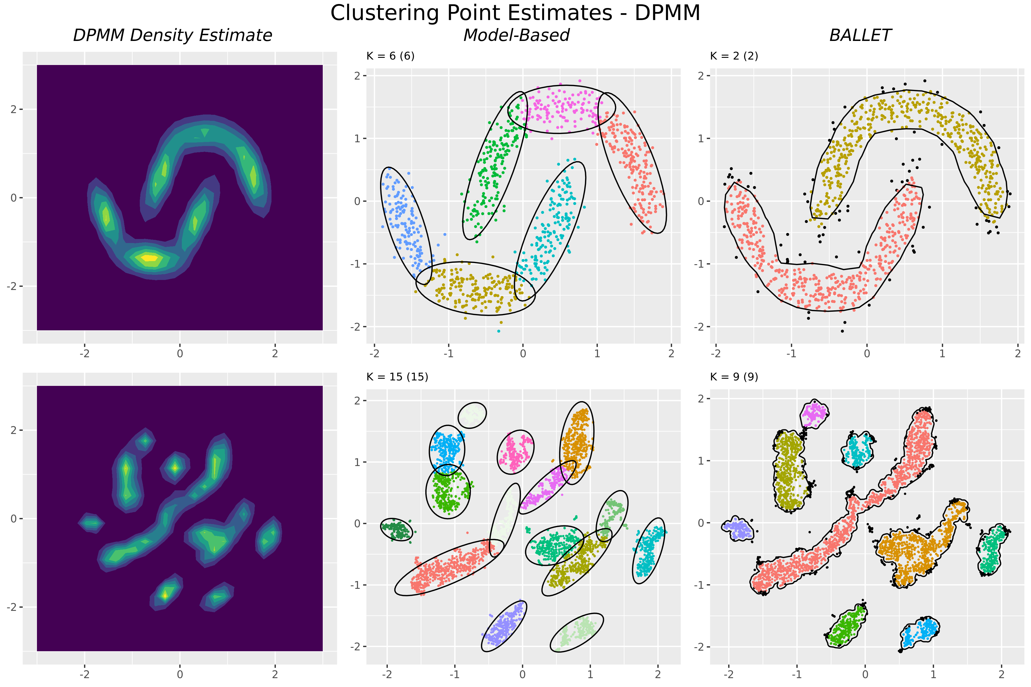
Figure 2: Results of applying a Dirichlet process mixture model to two of the toy challenge datasets. The first column shows a heatmap of $E[f|\mathcal{X}_{n}]$, the second shows estimated model-based clusters and the third shows our BALLET point estimate. The number of clusters is shown at the top of each plot, with the number of non-singleton clusters in parentheses.

An appealing aspect of density-based clustering is that it separates the objective of flexibly modeling the data from that of clustering - rather than being restricted to mixture models, we can use any of the many modern, computationally efficient density estimation models in the Bayesian toolbox, such as Adapive Polya Trees (APTs) (ma2017adaptive) and Nearest Neighbor Dirichlet Mixtures (NNDMs) (chattopadhyay2020nearest). In Figure S4, we visualize point estimates of the densities obtained using APTs and NNDMs as well as the BALLET posteriors extracted from their associated posterior distributions on $f$. We note that the results for the three datasets are consistent across density estimation models (APT, NNDM, and DPMM) showing the robustness of BALLET to the choice of our prior.

Of course, whenever there is incomplete concentration of the posterior there will be uncertainty in our point estimate. We can characterize this uncertainty in terms of interpretable bounds on a posterior credible ball, with only slight modifications to the method proposed by wade2018bayesian for characterizing uncertainty in partitions. We show these credible bounds for our DPMM analysis of the t-SNE data in Figure 3.

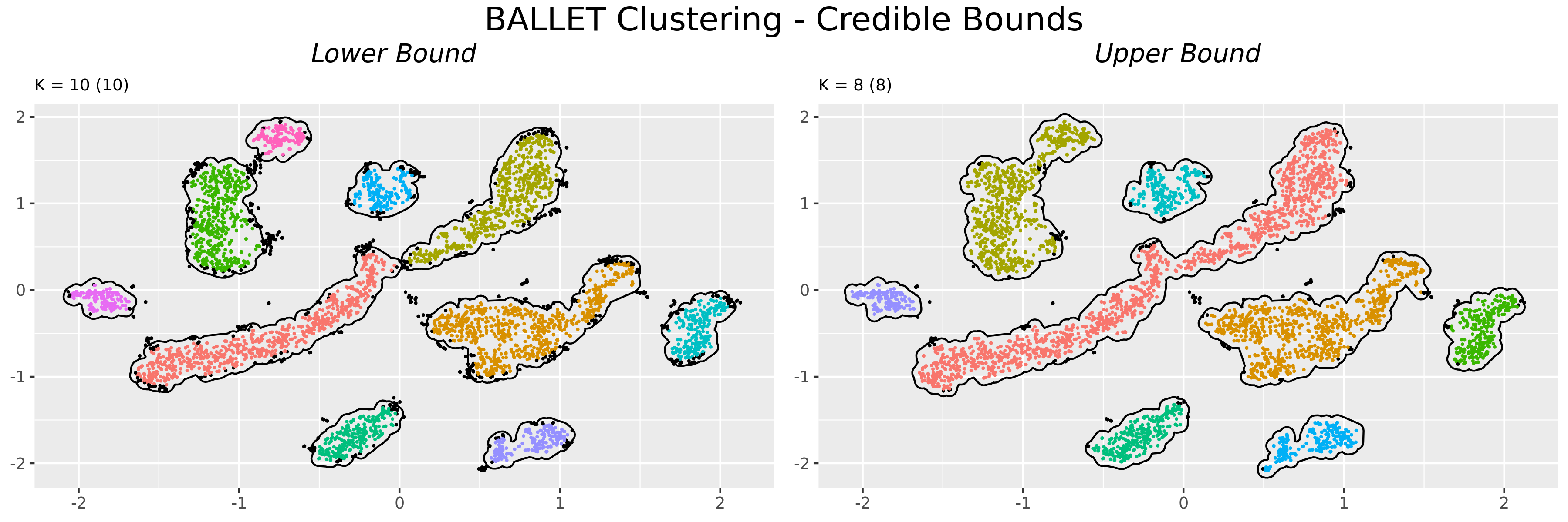
Figure 3: Upper and lower bounds for the 95% credible ball centered at our BALLET clustering estimate for the tSNE data, fit with the DPMM model for $f$. The cardinality of the partition is displayed in the title of each plot, as $K=X$, and it is followed, in parentheses by the count of clusters with more than 1 observation.

Additional results and figures specifically related to the analysis of the toy challenge datasets are collected in Supplementary Material S4.

6 Analysis of Astronomical Sky Survey Data

Astronomical sky survey data, such as the Sloan Digital Sky Survey, the 2dF Galaxy Redshift Survey, and the Edinburgh-Durham Southern Galaxy Catalogue (EDSGC) contain detailed images of the cosmos (see, for example, nichol1992edinburgh). One use for these data are to interrogate the density of matter in the universe. According to cosmological models, the mass and evolution of galaxy clusters over time should depend closely on the universal mass density $\Omega_{0}$ and hence, by analyzing the observable galaxy clusters we can make inferences about $\Omega_{0}$ (eke1998measuring).

At a given time $t$, we can model the distribution of galaxies in the universe as an inhomogeneous Poisson process with intensity function proportional to $\rho_{t}(x)$, where $\rho_{t}(x)$ denotes the mass density of objects at location $x$ (jang2003thesis). Specific values of $\Omega_{0}$ lead to predictions about the variability in $\rho_{t}(x)$, as characterized by the overdensity function, $\delta_{t}(x)=(\rho_{t}(x)-\bar{\rho}_{t})/\bar{\rho}_{t}$, where $\bar{\rho}_{t}$ is the mean density of mass in space. We can learn about $\Omega_{0}$ by characterizing the size and evolution of regions $\{x:\delta_{t}(x)\geq c\}$ for a scientifically motivated threshold $c$, believed to be around one (jang2003thesis). As noted by jang2006nonparametric, finding these regions is equivalent to estimating the level-set clusters of the density $f$ at the choice of level $\lambda=(c+1)\bar{f}$, where $f(x)\propto\rho_{t}(x)$ denotes the sampling density of the observed galaxies and $\bar{f}$ is the average density value.

Here we parallel the galaxy analysis of jang2006nonparametric as a proof-of-concept application of the BALLET clustering methodology. The data, provided to us by Woncheol Jang, are a cleaned subset of the complete EDSGC dataset (nichol1992edinburgh), and come with two catalogues of suspected cluster locations: the Abell catalogue (abell1989catalog) and the EDCCI (lumsden1992edinburgh). The Abell catalogue was created by visual inspection of the data by domain experts, while the EDCCI was produced by a custom-built cluster identification algorithm. These two catalogues serve as an imperfect ground truth: first of all, as jang2006nonparametric describes, they were known by their authors to be at least partially inaccurate; secondly, they identify each galaxy cluster with a single, central point, neglecting any differentiating information about shape and size; and thirdly, they include no characterization of uncertainty about their determinations. Nevertheless, they are useful in that they provide an opportunity for some external validation of our proposed clustering method.

To set the stage for our real-data analysis we conduct a simulation study, generating one hundred synthetic datasets designed to resemble the EDSGC data, analyzing them by the same BALLET methodology which will be used for the EDSGC data, and computing sensitivity and specificity in detecting regions with excess density. To accommodate the fact that target clusters are described only by their central point, we evaluate sensitivity and specificity based on small ellipses enclosing each estimated cluster: sensitivity is measured as the proportion of target points contained in at least one ellipse, while specificity is measured as the proportion of ellipses which contain a target point. Since sensitivity and specificity will both be equal to one if all the data points are assigned to a single cluster, we also computed a metric called exact match, defined as the fraction of ellipses that have exactly one target point.

As a competitor, we apply DBSCAN (ester1996density), which is perhaps the most popular level-set clustering algorithm.

6.1 Density Model and Tuning of Loss Parameters

In both the simulation study and real data analysis, we model the density $f$ with a simple mixture of random histograms: $f(x)=\sum_{k=1}^{K}\pi_{k}H_{k}(x;\mathcal{B}_{k},\bm{\rho}_{k})$, where $H_{k}(x;\mathcal{B}_{k},\bm{\rho}_{k})=\sum_{m=1}^{M}\mathds{1}_{\left[x\in B_{km}\right]}\rho_{km}$ is a histogram density with bins $\mathcal{B}_{k}=\{B_{k1},\dots,B_{kM}\}$ and weights $\bm{\rho}_{k}=\{\rho_{k1},\dots,\rho_{kM}\}$. We provide more details of our prior along with a fast approximation to sample from the posterior on $f$ in Supplementary Material S5.

Cosmological theory (see jang2006nonparametric) suggests the use of the threshold $\lambda=(1+c)\bar{f}$, where the constant $c$ is approximately one and $\bar{f}=\frac{\int_{\mathcal{X}}f(x)dx}{\operatorname{Vol}(\mathcal{X})}=1/\left(\operatorname{Vol}(\mathcal{X})\right)$ denotes the average value of $f$. We chose the value $c=1$ for our preliminary analysis of the real data, highlighting a direct application of level-set clustering. Similarly, in the simulation study, we assume knowledge of the fraction of noisy observations $\nu=\int_{\{f<\lambda\}}f(x)dx\in(0,1)$.

Having fixed the level $\lambda$ (or equivalently, the noise fraction $\nu$), we chose the loss parameter $\delta$ for BALLET using the procedure in Section 2.3 with the default choice $k=k_{0}=\lceil\log_{2}(n)\rceil$. This corresponds to the parameters $\texttt{MinPts}=k+1$ and $Eps=q_{1-\nu}(\{\delta_{k}(x_{i}):x_{i}\in\mathcal{X}_{n}\})$ in DBSCAN (ester1996density). Unlike BALLET, we found that the performance of DBSCAN in our simulation study was sensitive to the choice of parameter $k$ (see Figure S8). Thus we also present results from DBSCAN in Appendices S7 and S6 with the parameter value $\texttt{MinPts}=60$, chosen to optimize its performance on the simulation study. The optimized performance of DBSCAN was comparable to that of BALLET with the default value $k=k_{0}$. Here we present results for both methods with the default value of $k=k_{0}$ since, in general, metrics to tune hyper-parameters may not be available unless we have some access to the ground truth cluster labels.

6.2 Simulation Study

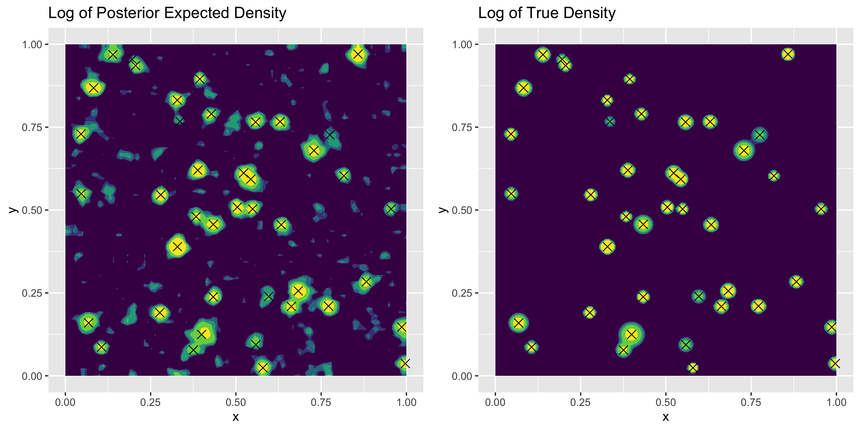
Figure S7: Comparison of $\log(\hat{f})$ and $f$, where $\hat{f}$ is the posterior expectation of $f$ under our mixture of random histograms model fitted to the data in Figure S6.

To mimic the EDSGC data, we simulated one hundred datasets, each drawn from a mixture distribution that placed $\nu=90\%$ of its mass on a uniform distribution over the unit square (the “noise component”), and divided the remaining 10% of its mass between 42 bivariate Gaussian components, with relative weights determined by a draw from a symmetric Dirichlet distribution with concentration parameter 1. The component means are sampled uniformly from the unit square, and the covariance is isotropic with variance drawn from a diffuse inverse gamma distribution. To sample our datasets, we randomly generated one hundred such mixture distributions and drew $n=40000$ independent and identically distributed observations from each mixture distribution, dropping any observations that fall outside the unit square. We plot a typical synthetic data set in Figure S6 and display the associated true and the estimated high-density regions in Figure S7.

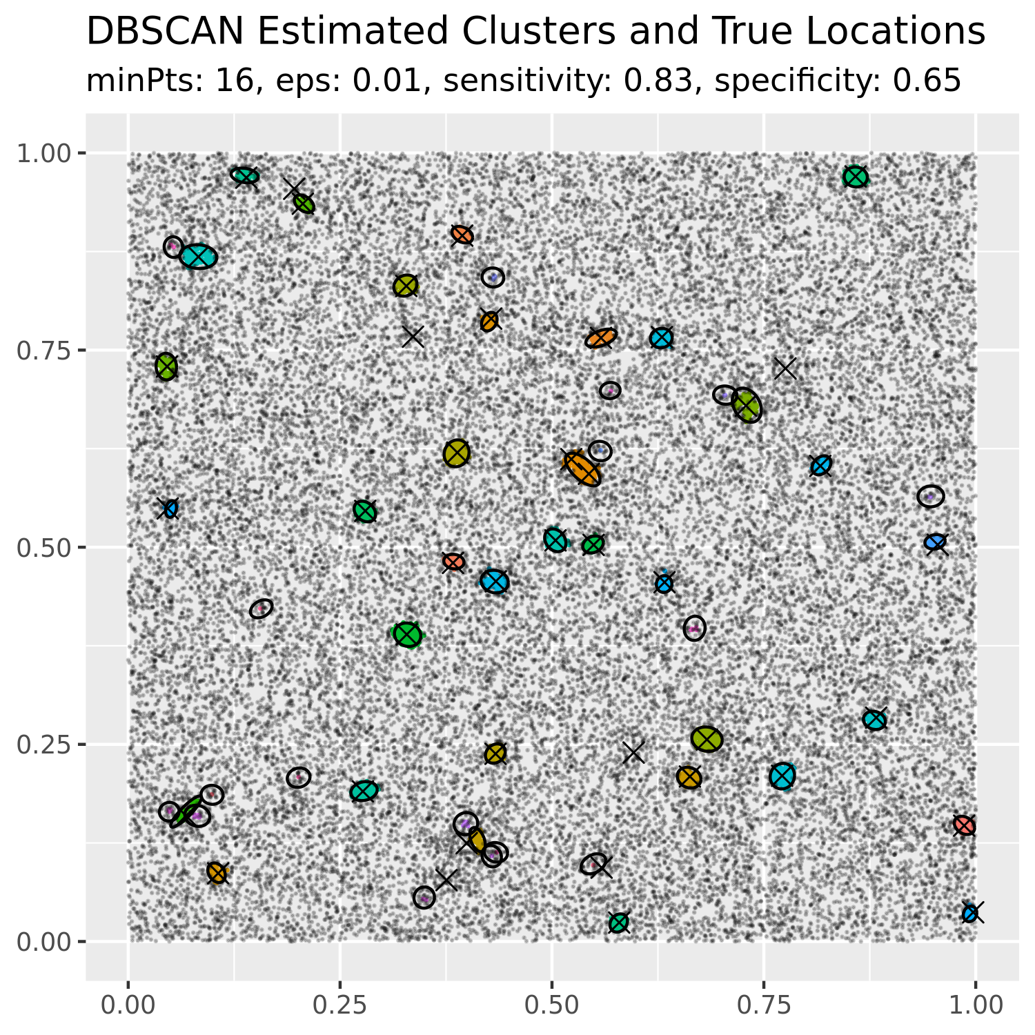
(a) DBSCAN clustering

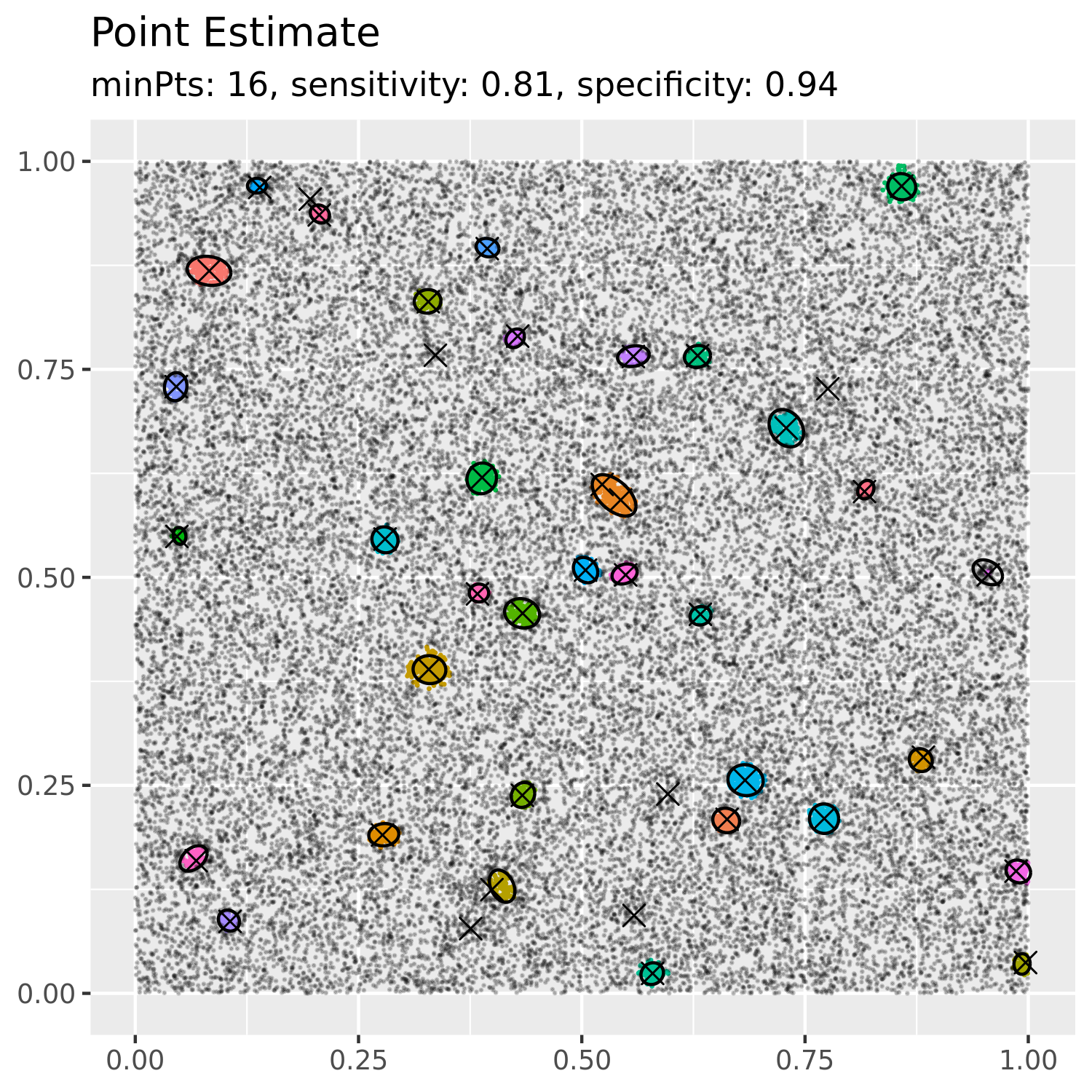
(b) BALLET Clustering

Figure 4: Clusters estimated by DBSCAN and BALLET for a representative synthetic sky survey dataset from our simulation study. We see an apparent preference of DBSCAN for detecting a large number of singleton or near-singleton clusters with the heuristic choice of its parameter $\texttt{MinPts}=k_{0}+1=16$.

In Figure 4, we show the result of applying DBSCAN and BALLET to our typical synthetic dataset, highlighting DBSCAN’s apparent preference for detecting a large number of singleton or near-singleton clusters given the heuristic choice of its parameter $\texttt{MinPts}=k_{0}+1=16$ and the known fraction of noise points $\nu=.9$.

The average performance of DBSCAN and BALLET clustering (point estimate and upper and lower bounds) over all the hundred datasets is shown in Table S1. DBSCAN achieved an average sensitivity of 0.86, but suffered from substantial false positives with an average specificity of 0.47 (exact match = 0.43). Meanwhile, BALLET achieved an average sensitivity of 0.79 while maintaining nearly perfect average specificity at 0.99 (exact match = 0.87). The BALLET lower and upper bounds performed more and less conservatively, respectively, than the point estimate. Particularly, on average, the BALLET lower bound had less sensitivity (.62) but more specificity (.99) and exact match (.9), while the BALLET upper bound had more sensitivity (.89) but less specificity (.97) and exact match (.83).

The performance of DBSCAN improved to match that of BALLET when its parameter $\texttt{MinPts}=k+1=60$ was chosen to maximize the sum of the sensitivity and specificity values (Table S1). On the other hand, we found that the performance of BALLET remained insensitive to the choice of $k$ (Figure S8). Thus while carefully tuning hyper-parameters based on the ground truth was necessary for DBSCAN to match the performance of BALLET, the performance of BALLET seems to be robust to our parameter choices. This may be because BALLET separates the act of careful data modeling from the task of computing its level set clusters.

6.3 Sky Survey Data Analysis

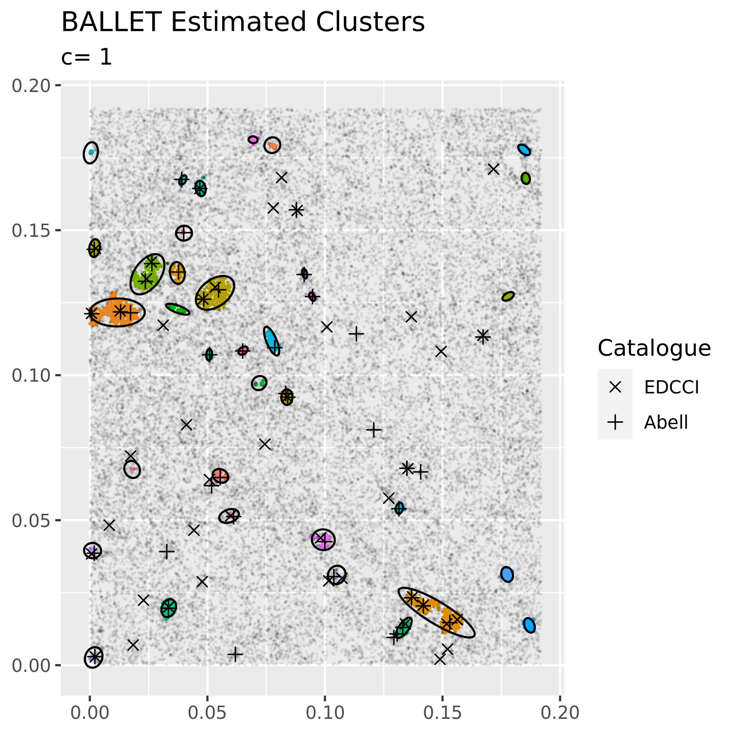
Figure S13: Results of applying BALLET Clustering to the EDSGC Data, with 95% credible bounds.

To provide a direct application for our level-set clustering methodology, we first applied DBSCAN and BALLET to the EDSGC data to estimate the clusters corresponding to the level $\lambda=2\bar{f}$, i.e. $c=1$. Having fixed $\lambda$ and thus the corresponding fraction of noise points $\nu$, we ran DBSCAN with the two values of its parameter MinPts of $k_{0}+1$ (the heuristic suggested in ester1996density) and $60$ (the value optimized based on our simulation study). The BALLET parameter $\delta$ was chosen as in Section 2.3 with $k_{0}=\lfloor\log_{2}(n)\rfloor=15$. The clusters estimated from the two methods can be found in Figures S13, S12 and S14.

	DBSCAN	DBSCAN1	BALLET Lower	BALLET Est.	BALLET Upper
Sensitivity	0.71	0.69	0.29	0.67	0.86
Specificity	0.25	0.63	0.87	0.69	0.42
Exact Match	0.23	0.45	0.67	0.51	0.32

Table 1: DBSCAN and BALLET Clustering coverage of the suspected galaxy clusters listed in the EDCCI catalogue. The column labeled “DBSCAN” reports the performance of the method with the standard, heuristically-chosen values of its tuning parameters, while “DBSCAN¹” shows the performance of the method with the optimal value of $\texttt{MinPts}=60$ chosen based on consideration of the ground truth in our simulation study.

Table 1 compares the clusters obtained by the two methods to the EDCCI catalogue of suspected galaxy clusters. While DBSCAN with the heuristic parameter choice detected 71 percent of the EDCCI clusters, the method only had a specificity of 25 percent. In contrast, DBSCAN with the optimized parameter choice fared better: finding 69 percent of the EDCCI clusters with a specificity of 63 percent. Meanwhile, BALLET recovered 67 percent of the EDCCI clusters and had a specificity of 69 percent. Both DBSCAN and BALLET detected only 40 percent of the clusters listed in the Abell catalogue (see Table S2), but again BALLET was much more specific than DBSCAN with the heuristic parameter choice, scoring 40 percent rather than 18 percent. It is encouraging to see that both methods performed better at recovering the suspected galaxy clusters in the EDCCI than the Abell catalogue, as the former is considered to be more reliable (jang2006nonparametric).

Figure 5 visualizes the BALLET clustering uncertainty (Section 3) by showing the upper and lower bounds for a 95 percent credible ball around the point estimate. The lower bound has fewer and smaller clusters, and tends to include locations that the EDCCI and Abell catalogs agree on. In contrast, the upper bound has larger and more numerous clusters, and tends to include many of the suspected cluster locations from both the catalogs.

Thus, the BALLET upper and lower bounds summarize the clustering uncertainty in this problem, with the lower bound providing a conservative estimate of the clusters and the upper bound providing an overestimate for the possible clusters. Indeed, based on Tables 1 and S2, one may suspect that the 14 percent EDCCI locations and 44 percent Abell locations that were not discovered by the BALLET upper bound may be erroneous. Complementarily, we may have high confidence in the 21 percent locations in Abell and the 29 percent locations in EDCCI which were discovered by the BALLET lower bound.

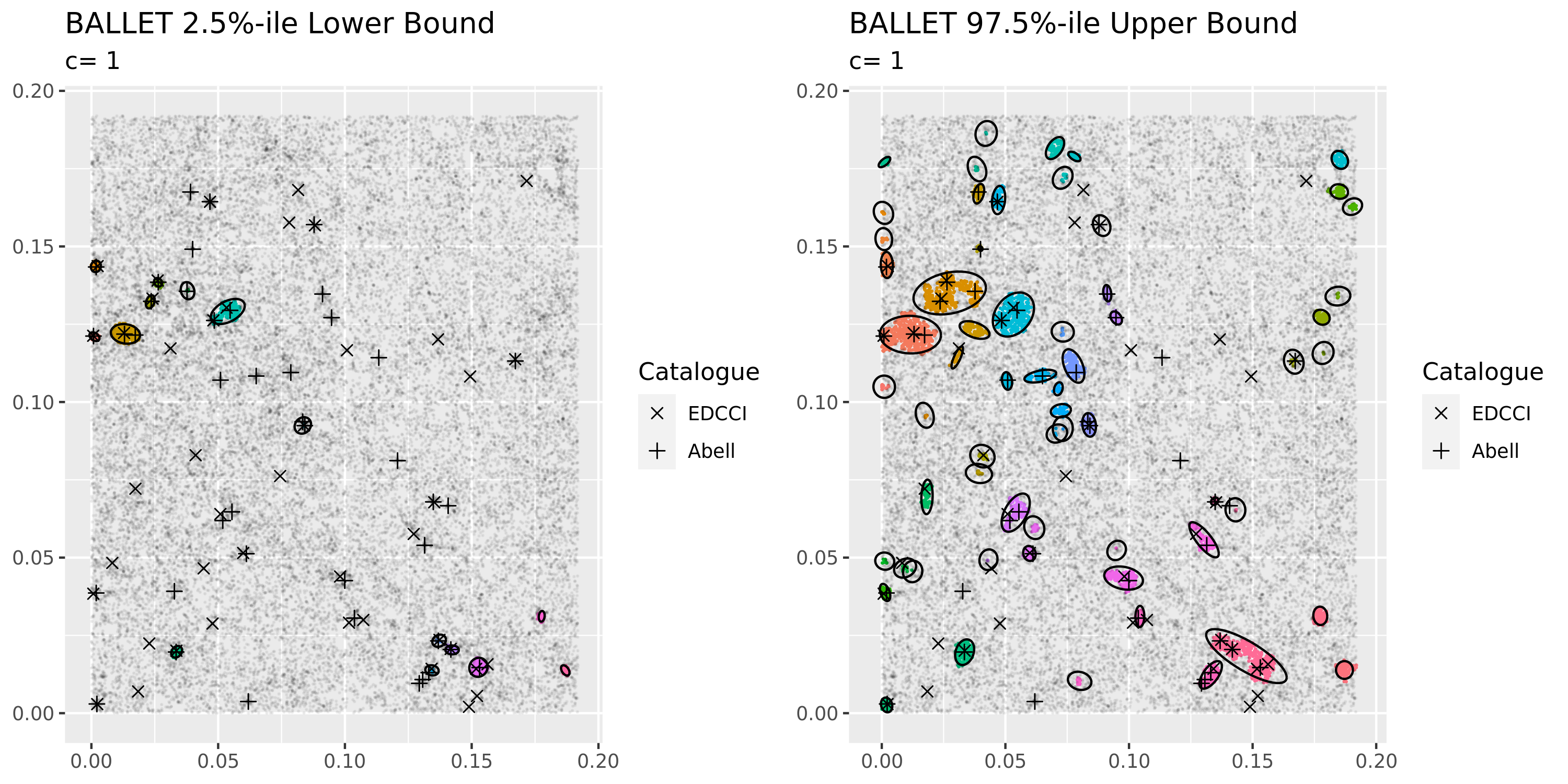
Figure 5: Upper and lower bounds of the 95% credible ball centered at our BALLET estimate of the galaxy clusters in the EDSGC data.

7 Discussion

In this article, we developed a Bayesian approach to level-set clustering. Our key idea has been to use Bayesian decision theory to separate the part of modeling the data density from that of identifying clusters.

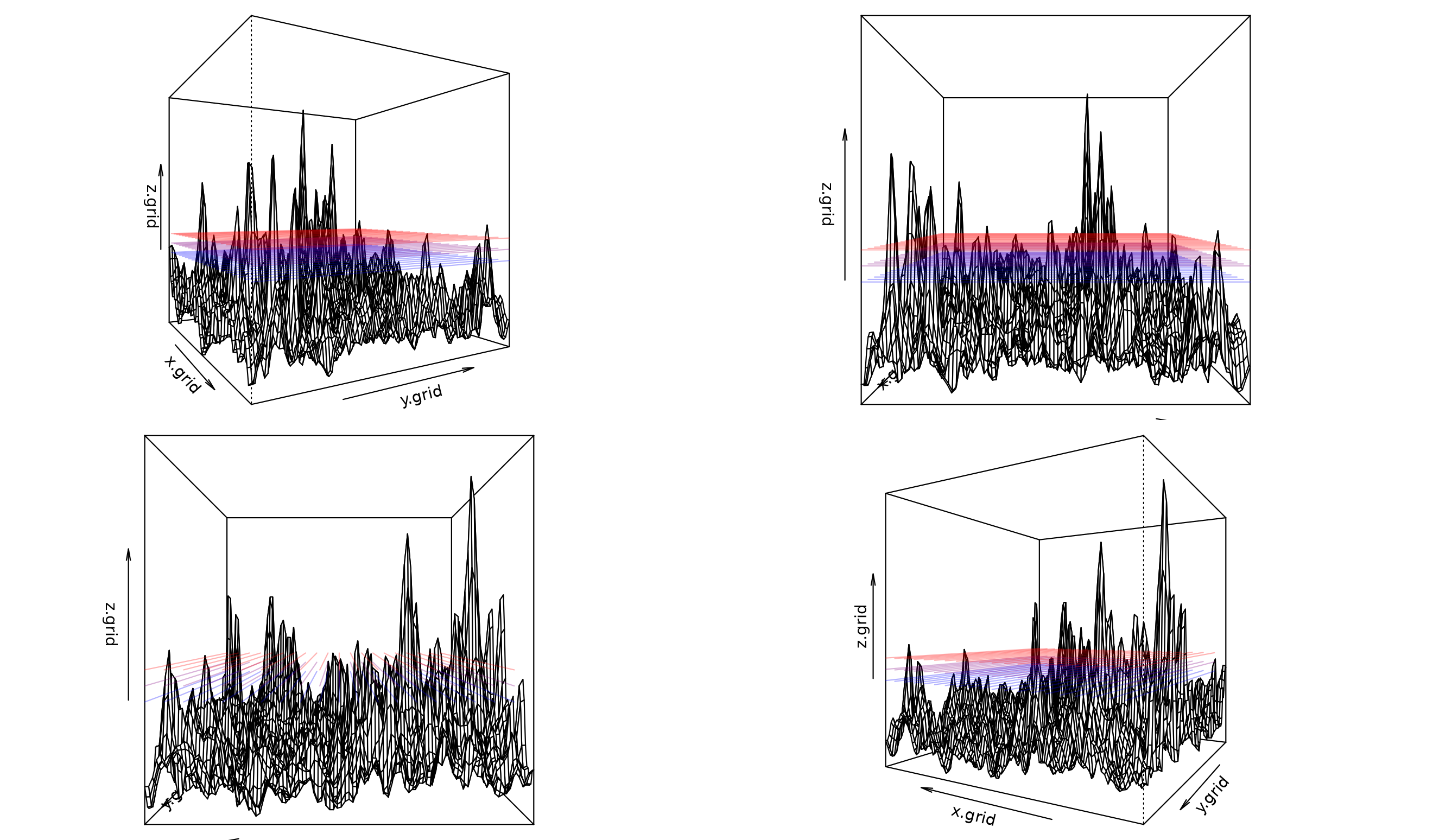
Figure 6: Visualizing our density estimate (plotted on the z-axis) for the Sky Survey data. The colored lines mark the choice of different levels corresponding to the values of $c\in\{.8,1,1.2\}$. The level-set clusters are seen to be sensitive to the exact choice of $c$.

While level-set clustering is a popular and conceptually appealing clustering framework, one of its key practical challenges is the choice of the level $\lambda>0$ (campello2020density). Particularly, in many applications, the level of interest may not be known in advance or it may be known (or estimated) only in an approximate way. Thus, the sensitivity of a level-set clustering method to the exact choice of $\lambda$ is an important practical concern. Indeed, based on visualizing the density estimate for our sky survey data (Figure 6), we find the level-set clusters will be sensitive to the exact value of the scientific constant $c$.

To reduce sensitivity to $\lambda$, we describe a persistent clustering approach in Supplementary Material S8 that computes BALLET clusters for various values of $c$ in the interval $[.8,1.2]$ and visualizes these clusters in the form of a cluster tree (clustree). This tree is then processed to extract a flat clustering made up of clusters that remained active or persistent across all the levels in the tree. We found that this approach improved our specificity in detecting the two catalogs without losing sensitivity.

Finally, while we have focused on level set clustering as an important initial case, our Bayesian density-based clustering framework is broad and motivates multiple directions for future work. One possibility is to avoid focusing on a single threshold $\lambda$, but instead estimate an entire cluster tree obtained by varying the threshold. Loss functions introduced by fowlkes1983method may provide a relevant starting point.

An alternative direction is to target a single clustering, but vary the threshold $\lambda$ over the observation space in a data-adaptive manner (campello2020density). Varying $\lambda$ is important in uncovering distinct cluster structures at varying levels of the density without inferring the full cluster tree; refer, for example, to the illustrative example in Figure S17.

A more dramatic departure from our proposed BALLET would be to target density-based clusters that are not based on level sets. A natural direction is this respect is mode-based clustering, which regards clusters as basins of attraction around local modes (menardi2016modal; chen2016comprehensive). Substantial challenges in using our framework for Bayesian mode-based clustering include: (1) efficiently partitioning the sample space based on basins of attraction around local modes; and (2) avoiding sensitivity to artifactual extra modes introduced in Bayesian density estimation; refer, for example to Figure 1.

Supplementary Materials

The accompanying supplementary materials contain additional details, including figures and tables referenced in the article starting with the letter ‘S’. Code to reproduce our analysis can be found online at https://github.com/davidbuch/ballet_article.

Supplementary Material for “Bayesian Level-Set Clustering”

Appendix S1 Related Work

The last two decades have witnessed a significant maturation of the Bayesian clustering literature (medvedovic2002bayesian; fritsch2009improved; wade2018bayesian; rastelli2018optimal; dahl2022search). By designing and characterizing loss functions on partitions and developing search algorithms to identify partitions which minimize Bayes risk, these articles and others have established a sound framework for Bayesian decision theoretic clustering. This literature acknowledges the cluster-splitting problem alluded to in our preceding discussion, with (wade2018bayesian) and (dahl2022search) finding that clustering point estimates obtained by minimizing Bayes risk under certain parsimony-encouraging loss functions are less prone to cluster-splitting.

However, these loss functions cannot completely eliminate the problem. (guha2021posterior) shows that a fundamental cause of cluster-splitting is that Bayesian mixture models converge to the mixture that has minimum Kullback-Leibler divergence to the true density. When the mixture components are misspecified, it may require infinitely many parametric components to recapitulate the true data-generating density. Thus, as data accumulate, it would seem to be futile to attempt to overcome the cluster-splitting problem merely by encouraging parsimony in the loss function. If the components are at all misspecified, as data accumulate, eventually the preponderance of evidence will insist on splitting the clusters to reflect the multiplicity of parametric components. As further support for our heuristic argument, note that in our illustrative example in Figure 1 (a) we actually used the parsimony-encouraging Variation of Information (VI) loss to obtain the Gaussian mixture model-based clustering point estimate.

One response to this problem is the coarsened Bayes methodology of (miller2018robust), which conditions only on the mixture model being approximately correctly specified. Another approach to mitigate the problem is to expand the class of mixture components (fruhwirth2010bayesian; malsiner2017identifying; stephenson2019robust). As we have claimed above, naive applications of this strategy can lead to loss of practical identifiability and computational challenges, though (dombowsky2023bayesian) have had some success increasing component flexibility indirectly by merging nearby less-flexible mixture components in a post-processing step. The generalized Bayes paradigm, introduced by (bissiri2016general), also provides an answer to the cluster splitting problem via a loss-function-based Gibbs posterior for clustering (rigon2020generalized).

The idea of framing Bayesian clustering as a problem of computing a risk-minimizing summary, $\psi$, of the posterior distribution on density $f$ can be viewed as related to the existing literature on decision theoretic summaries of posterior distributions (woody2021model; afrabandpey2020decision; ribeiro2018anchors), though this literature has focused on extracting interpretable conclusions from posterior distributions on regression surfaces. In contrast, clustering in the manner we have proposed extracts an interpretable summary from a posterior distribution on the data generating density. In addition, while authors in that literature focus on the interpretability of summary functions $\psi$, we use the clustering example to emphasize that ideally $\psi$ should also be robust, in the sense that $\psi(f^{*})$ will be close to $\psi(f)$ when $f^{*}$ is close to $f$, since this would suggest small amounts of prior bias or model misspecification would not lead to large estimation errors.

The general framework of density-based clustering could be used to target other meaningful partitions of the observations and sample space. For example, clustering functions $\psi$ which return the basins of attraction of modes of $f$, based on literature contributions such as (chen2016comprehensive), could provide methods for modal clustering. Currently, such approaches face substantial computational challenges (dahl2009modal). For level-set clustering specifically, there is both an expansive algorithmic (ester1996density; schubert2017dbscan; campello2020density) and frequentist literature (cuevas2000estimating; jang2006nonparametric; sriperumbudur2012consistency; rinaldo2010generalized). However, the frequentist approach relies primarily on kernel density estimation (silverman2018density) while the algorithmic literature often implicitly adopts a nearest neighbors density estimate (biau2015lectures).

Appendix S2 The lattice of sub-partitions

The space of sub-partitions $\mathscr{P}(\mathcal{X})$ forms a lattice under the partial order given by $\bm{C}\preceq\bm{C}^{\prime}$ if and only if there is a map $\phi:\bm{C}\to\bm{C}^{\prime}$ such that $C\subseteq\phi(C)$ for each $C\in\bm{C}$. One can check that $(\mathscr{P}(\mathcal{X}),\preceq)$ with join $\bm{C}\vee\bm{C}^{\prime}\doteq\{C\cup C^{\prime}|C\in\bm{C},C^{\prime}\in\bm{C}^{\prime},C\cap C^{\prime}=\emptyset\}$ and meet $\bm{C}\wedge\bm{C}^{\prime}=\{C\cap C^{\prime}|C\in\bm{C},C^{\prime}\in\bm{C}^{\prime},C\cap C^{\prime}=\emptyset\}$ is a lattice.

We denote $\bm{C}\prec\bm{C}^{\prime}$ if $\bm{C}\preceq\bm{C}^{\prime}$ but it is not the case that $\bm{C}^{\prime}\preceq\bm{C}$. We can define a Hasse diagram for this lattice based on the relation $\bm{C}\rightarrow\bm{C}^{\prime}$ if $\bm{C}\prec\bm{C}^{\prime}$ but there is no $\bm{C}^{\prime\prime}\in\mathscr{P}(\mathcal{X})$ such that $\bm{C}\prec\bm{C}^{\prime\prime}\prec\bm{C}^{\prime}$. One can show that $\bm{C}\rightarrow\bm{C}^{\prime}$ if and only if one of the following conditions hold:

• $\bm{C}^{\prime}$ is obtained by merging two active clusters in $\bm{C}$. That is, after suitable reordering: $\bm{C}=\{C_{1},\ldots,C_{k}\}$ and $\bm{C}^{\prime}=\{C_{1}\cup C_{2}\}\cup\{C_{r}:r\in\{3,\ldots,k\}\}$.

• $\bm{C}^{\prime}$ is obtained by adding a noise point to its own cluster: i.e., $\bm{C}^{\prime}=\bm{C}\cup\{{n}\}$ for some $n\in\mathcal{X}$ that is not active in $\bm{C}$.

This relation allows us to construct an Hasse diagram: a directed acyclic graph with nodes $\mathscr{P}(\mathcal{X})$ and edges given by the relation $\rightarrow$. This diagram has the property that $\bm{C}\prec\bm{C}^{\prime}$ if and only if there is a path from $\bm{C}$ to $\bm{C}^{\prime}$. The Hasse diagram for the lattice of sub-partitions of $\mathcal{X}=\{1,2,3\}$ is shown in Figure S1.

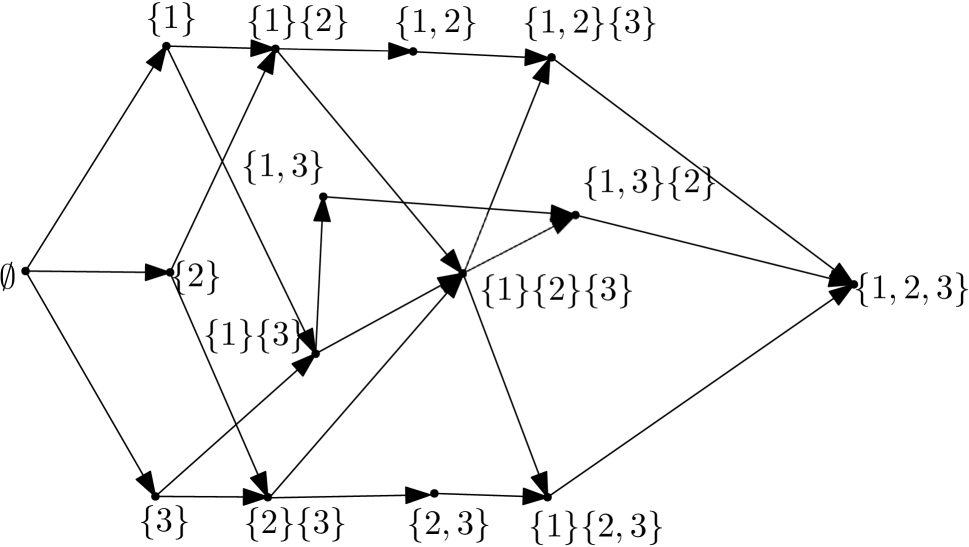
Figure S1: Hasse diagram for the lattice of sub-partitions $\mathscr{P}(\mathcal{X})$ of the space $\mathcal{X}=\{1,2,3\}$. This diagram has the property that $\bm{C}\prec\bm{C}^{\prime}$ if and only if there is a path from $\bm{C}$ to $\bm{C}^{\prime}$.

Appendix S3 Proofs from Section 4

We now provide proofs of the results in Section 4. We begin with a proof of Theorem 1 followed by the proofs of the two lemmas in Section 4.2.

Proof of Theorem 1

The proof is a simple application of the metric properties of $D$. In particular, note that

$$D(\widehat{\psi}_{M}(\mathcal{X}_{n}),\psi(f_{0})) \leq E_{f\sim P_{M}(\cdot|\mathcal{X}_{n})}D(\widetilde{\psi}(f),\psi(f_{0}))+E_{f\sim P_{M}(\cdot|\mathcal{X}_{n})}D(\widetilde{\psi}(f),\widehat{\psi}_{M}(\mathcal{X}_{n}))$$

$$\leq 2E_{f\sim P_{M}(\cdot|\mathcal{X}_{n})}D(\widetilde{\psi}(f),\psi(f_{0}))$$

where the first line follows by taking expectation with respect to the posterior distribution $P_{M}(\cdot|\mathcal{X}_{n})$ after using the triangle inequality and symmetry for the metric $D$, while the second line follows by noting that the second term in the right hand side of the first line is no greater than the first term, since $\widehat{\psi}_{M}(\mathcal{X}_{n})$ is given by (7). Noting further that $D$ is bounded above by one, we obtain

$$E_{f\sim P_{M}(\cdot|\mathcal{X}_{n})}D(\widetilde{\psi}(f),\psi(f_{0})) \leq P_{M}\left(f:\|f-f_{0}\|_{\infty}>K_{n}\epsilon_{n}|\mathcal{X}_{n}\right)+\sup_{f:\|f-f_{0}\|_{\infty}\leq K_{n}\epsilon_{n}}D(\widetilde{\psi}(f),\psi(f_{0}))$$

$$=\delta_{1}(\mathcal{X}_{n})+\delta_{2}(\mathcal{X}_{n})$$

where $\delta_{1}$ is defined in Assumption 2 and $\delta_{2}$ and constant $K_{n}$ are as defined in Assumption 3. Since $K_{n}\to\infty$, these assumptions show that $\delta_{1}(\mathcal{X}_{n}),\delta_{2}(\mathcal{X}_{n})\overset{P}{\to}0$ as $n\to\infty$.

Verifying Assumptions 3 and 1 for BALLET estimators

We provide proofs of Lemmas 1 and 2 from Section 4.2 in the next two subsections.

S3.1 Proof of Lemma 1

It order to simplify the presentation of our proof we first introduce some notation. We note that any sub-partition $\bm{C}=\{C_{1},\ldots,C_{k}\}\in\mathscr{P}(\mathcal{X}_{n})$ defines a binary “co-clustering” relation $\bm{C}_{R}:\mathcal{X}_{n}\times\mathcal{X}_{n}\to\{0,1\}$ on pairs of data points, namely

$$\bm{C}_{R}(x,y)\doteq\mathds{1}_{\left[x\notin A,y\notin A\right]}+\sum_{h=1}^{k}\mathds{1}_{\left[x\in C_{h},y\in C_{h}\right]}$$

where $A=\cup_{h=1}^{k}C_{h}$ is the set of active points in $\bm{C}$. In other words, $\bm{C}_{R}(x,y)=1$ if $x,y\in\mathcal{X}_{n}$ are both noise points, or if they belong to a common cluster in $\bm{C}$, and $\bm{C}_{R}(x,y)=0$ otherwise. Given $\bm{C}$, we can also obtain an indicator function of active points $\bm{C}_{A}:\mathcal{X}_{n}\to\{0,1\}$ such that $\bm{C}_{A}(x)=1$ if and only if $x\in A$. In fact, knowing the binary functions $\bm{C}_{R}$ and $\bm{C}_{A}$ is sufficient to uniquely recover the sub-partition $\bm{C}\in\mathscr{P}(\mathcal{X}_{n})$. Indeed, this follows because $\bm{C}_{R}$ is an equivalence relation on $\mathcal{X}_{n}$, and the sub-partition $\bm{C}$ can be recovered by dropping the inactive subset $\bm{C}_{A}^{-1}(0)$ from the equivalence partition of $\mathcal{X}_{n}$ induced by $\bm{C}_{R}$.

We also introduce the following subscript-free notation for summation of a symmetric function $F:\mathcal{X}_{n}\times\mathcal{X}_{n}\to\mathbb{R}$ over pairs of distinct data points that lie in $S\subseteq\mathcal{X}$:

$$\sum_{x\neq y\in\mathcal{X}_{n}\cap S}F(x,y)\doteq\sum_{\begin{subarray}{c}1\leq i<j\leq n\\ x_{i},x_{j}\in S\end{subarray}}F(x_{i},x_{j})=\frac{1}{2}\sum_{\begin{subarray}{c}i,j\in[n]\\ x_{i},x_{j}\in S\end{subarray}}F(x_{i},x_{j})\mathds{1}_{\left[i\neq j\right]}.$$

Proof of Lemma 1.

Similar to analyses of Binder’s loss, the first step in our proof is to note that $L_{\text{IA-Binder}}$ can be written as a sum of pairwise losses $\phi_{x,y}$ over pairs $x,y\in\mathcal{X}_{n}$. In particular, fix any $\bm{C},\bm{C}^{\prime}\in\mathscr{P}(\mathcal{X}_{n})$, and let $A=\bm{C}_{A}^{-1}(1)$, $A^{\prime}=\bm{C}_{A}^{{}^{\prime}-1}(1)$ and $I=\bm{C}_{A}^{-1}(0)$, $I^{\prime}=\bm{C}_{A}^{{}^{\prime}-1}(0)$ denote the active and inactive sets of $\bm{C}$ and $\bm{C}^{\prime}$ , respectively. Taking $a=b$ and $m=m_{ia}=m_{ai}$ in (2.4), we note

$$L_{\text{IA-Binder}}(\bm{C},\bm{C}^{\prime}) =m(n-1)(|A\cap I^{\prime}|+|I\cap A^{\prime}|)+a\sum_{\begin{subarray}{c}1\leq i<j\leq n\\ x_{i},x_{j}\in A\cap A^{\prime}\end{subarray}}\mathds{1}_{\left[\bm{C}_{R}(x_{i},x_{j})\neq\bm{C}^{\prime}_{R}(x_{i},x_{j})\right]}$$

$$=\sum_{x\neq y\in\mathcal{X}_{n}}\phi_{x,y}(\bm{C},\bm{C}^{\prime})$$ (S1)

where

$$\small\phi_{x,y}(\bm{C},\bm{C}^{\prime})=m\mathds{1}_{\left[\bm{C}_{A}(x)\neq\bm{C}_{A}^{\prime}(x)\right]}+m\mathds{1}_{\left[\bm{C}_{A}(y)\neq\bm{C}_{A}^{\prime}(y)\right]}+a\mathds{1}_{\left[\bm{C}_{R}(x,y)\neq\bm{C}^{\prime}_{R}(x,y)\right]}\mathds{1}_{\left[\bm{C}_{A}(x)=\bm{C}_{A}^{\prime}(x)=\bm{C}_{A}(y)=\bm{C}_{A}^{\prime}(y)\right]}.$$

In order to obtain (S1), we have used the fact that the last term in $\phi_{x,y}(\bm{C},\bm{C}^{\prime})$ is zero when either one of $x$ or $y$ is outside the set $A\cap A^{\prime}$, and the fact that the summation $\Sigma_{x\neq y\in\mathcal{X}_{n}}$ over the first two terms in $\phi_{x,y}(\bm{C},\bm{C}^{\prime})$ is equal to $m(n-1)(|A\cap I^{\prime}|+|I\cap A^{\prime}|)$.

Now we shall use (S1) to show that $D=\binom{n}{2}^{-1}L_{\text{IA-Binder}}$ is a metric that is bounded above by one when $a,m\leq 1$. Note that at most one out of the three indicator variables in $\phi_{x,y}$ can be non-zero for any instance, and hence $\phi_{x,y}$ is bounded above by one (in fact by $\max(a,m)\leq 1$) for each of the $\binom{n}{2}$ summation variables $x\neq y\in\mathcal{X}_{n}$. This shows that $D$ is also bounded above by one. Further, the symmetry of $D$ in its arguments follows from the symmetry of $\phi_{x,y}$ in its arguments for every $x\neq y\in\mathcal{X}_{n}$.

Next suppose $D(\bm{C},\bm{C}^{\prime})=0$. Since the functions $\phi_{x,y}$ are non-negative, this shows that $\phi_{x,y}(\bm{C},\bm{C}^{\prime})=0$ for each $x\neq y\in\mathcal{X}_{n}$. Since $2m\geq a>0$, the functions $\bm{C}_{A}$ and $\bm{C}^{\prime}_{A}$ are equal (or equivalently that $A=A^{\prime}$), and further that $\bm{C}_{R}(x,y)=\bm{C}^{\prime}_{R}(x,y)$ either when $x,y\in A=A^{\prime}$ or $x,y\in I=I^{\prime}$. The latter condition is sufficient to show that the relations $\bm{C}_{R}$ and $\bm{C}^{\prime}_{R}$ are equal since $\bm{C}_{R}(x,y)=0=\bm{C}^{\prime}_{R}(x,y)$ when $x\in A,y\in I$ or $x\in I,y\in A$. Since the binary functions $\bm{C}_{A}$ and $\bm{C}_{R}$ determine the sub-partition $\bm{C}$, we have $\bm{C}=\bm{C}^{\prime}$.

Finally, to demonstrate that $D$ satisfies the triangle inequality, it suffices to show that for each $x\neq y\in\mathcal{X}_{n}$, we have the triangle inequality $\phi_{x,y}(\bm{C},\bm{C}^{\prime\prime})\leq\phi_{x,y}(\bm{C},\bm{C}^{\prime})+\phi_{x,y}(\bm{C}^{\prime},\bm{C}^{\prime\prime})$ for any sub-partitions $\bm{C},\bm{C}^{\prime},\bm{C}^{\prime\prime}\in\mathscr{P}(\mathcal{X}_{n})$. Indeed when either $\bm{C}_{A}(x)\neq\bm{C}^{\prime\prime}_{A}(x)$ or $\bm{C}_{A}(y)\neq\bm{C}^{\prime\prime}_{A}(y)$, the triangle inequality for $\phi_{x,y}$ follows from the inequality:

$$\mathds{1}_{\left[\bm{C}_{A}(z)\neq\bm{C}_{A}^{\prime\prime}(z)\right]} \leq\mathds{1}_{\left[\bm{C}_{A}(z)\neq\bm{C}_{A}^{\prime}(z)\right]}+\mathds{1}_{\left[\bm{C}^{\prime}_{A}(z)\neq\bm{C}_{A}^{\prime\prime}(z)\right]}\qquad z\in\{x,y\}.$$

Otherwise, let us assume that the previous condition does not hold. Let us further suppose that $\phi_{x,y}(\bm{C},\bm{C}^{\prime\prime})>0$ or else there is nothing to show. This means that we are under the case $\phi_{x,y}(\bm{C},\bm{C}^{\prime\prime})=a$, $\bm{C}_{A}(x)=\bm{C}^{\prime\prime}_{A}(x)=\bm{C}_{A}(y)=\bm{C}^{\prime\prime}_{A}(y)$, and $\bm{C}_{R}(x,y)\neq\bm{C}^{\prime\prime}_{R}(x,y)$. If $\bm{C}^{\prime}_{A}(x)\neq\bm{C}_{A}(x)=\bm{C}^{\prime\prime}_{A}(x)$ (or analogously $\bm{C}^{\prime}_{A}(y)\neq\bm{C}_{A}(y)=\bm{C}^{\prime\prime}_{A}(y)$) then the triangle inequality is satisfied as $\phi_{x,y}(\bm{C},\bm{C}^{\prime})+\phi_{x,y}(\bm{C}^{\prime},\bm{C}^{\prime\prime})\geq m\mathds{1}_{\left[\bm{C}_{A}(x)\neq\bm{C}_{A}^{\prime}(x)\right]}+m\mathds{1}_{\left[\bm{C}^{\prime}_{A}(x)\neq\bm{C}_{A}^{\prime\prime}(x)\right]}=2m\geq a=\phi_{x,y}(\bm{C},\bm{C}^{\prime\prime})$. Otherwise, the only remaining case is that $\bm{C}_{A}(x)=\bm{C}^{\prime}_{A}(x)=\bm{C}^{\prime\prime}_{A}(x)=\bm{C}_{A}(y)=\bm{C}^{\prime}_{A}(y)=\bm{C}^{\prime\prime}_{A}(x)$. Then the triangle inequality is satisfied since

$$\phi_{x,y}(\bm{C},\bm{C}^{\prime\prime})=a\mathds{1}_{\left[\bm{C}_{R}(x,y)\neq\bm{C}^{\prime\prime}_{R}(x,y)\right]} \leq a\mathds{1}_{\left[\bm{C}_{R}(x,y)\neq\bm{C}^{\prime}_{R}(x,y)\right]}+a\mathds{1}_{\left[\bm{C}^{\prime}_{R}(x,y)\neq\bm{C}^{\prime\prime}_{R}(x,y)\right]}$$

$$=\phi_{x,y}(\bm{C},\bm{C}^{\prime})+\phi_{x,y}(\bm{C}^{\prime},\bm{C}^{\prime\prime}).$$

Hence, we have verified the triangle inequality for $\phi_{x,y}$, and hence also for $D$. Combined with the non-negativity of $D$, we have shown that $D$ is a metric. ∎

S3.2 Proof of Lemma 2

Letting $\mathcal{X}=\mathbb{R}^{d}$, we begin with the necessary assumptions on the unknown data density $f_{0}:\mathcal{X}\to\mathbb{R}$ and the threshold level $\lambda>0$.

S3.2.1 Assumptions on $f_{0}$ and level $\lambda$

Let $S_{\lambda}=\{x\in\mathbb{R}^{d}:f_{0}(x)\geq\lambda\}$ denote the level set of the unknown data density $f_{0}$ at threshold $\lambda\in(0,\infty)$. We make the following assumptions.

Assumption S4.

(Continuity with vanishing tails) The density $f_{0}:\mathbb{R}^{d}\to[0,\infty)$ is continuous and satisfies $\lim_{\|x\|\to\infty}f_{0}(x)=0$.

Lemma S1.

If Assumption S4 holds, then $f_{0}$ is uniformly continuous.

Proof.

Fix any $\epsilon>0$. Then since $f_{0}$ has vanishing tails, there is a $K>0$ such that $\sup_{x\in\mathbb{R}^{d}\setminus([-K,K]^{d})}f_{0}(x)\leq\epsilon/2$, and since $f_{0}$ is continuous on the compact set $H=[-K-1,K+1]^{d}$, there is a $\delta\in(0,1)$ such that $|f_{0}(x)-f_{0}(y)|\leq\epsilon$ whenever $\|x-y\|\leq\delta$ and $x,y\in H$. Finally if $x,y\in\mathbb{R}^{d}$ are such that $\|x-y\|\leq 1$ and $\{x,y\}\cap\mathbb{R}^{d}\setminus H\neq\emptyset$ then $x,y\in\mathbb{R}^{d}\setminus[-K,K]^{d}$. Thus $|f_{0}(x)-f_{0}(y)|\leq f_{0}(x)+f_{0}(y)\leq\epsilon/2+\epsilon/2=\epsilon$. Hence we have shown that there is a $\delta\in(0,1)$ such that $|f_{0}(x)-f_{0}(y)|\leq\epsilon$ whenever $\|x-y\|\leq\delta$ and $x,y\in\mathbb{R}^{d}$. Since $\epsilon>0$ is arbitrary, we have shown that $f_{0}$ is uniformly continuous. ∎

Assumption S5.

(Fast mass decay around level $\lambda$) There are constants $C,\bar{\varepsilon}>0$ such that $\int_{\{x\in\mathbb{R}^{d}:|f_{0}(x)-\lambda|\leq\epsilon\}}f_{0}(x)dx\leq C\epsilon$ for all $\epsilon\in(0,\bar{\varepsilon})$.

Assumption S5 is adapted from (rinaldo2010generalized), and intuitively prevents the density from being too flat around the level $\lambda$. In particular, if $f_{0}$ satisfies $\|\nabla f_{0}(x)\|>0$ for Lebesgue-almost-every $x$, then Lemma 4 in (rinaldo2010generalized) shows that Assumption S5 will hold for Lebesgue-almost-every $\lambda\in(0,\|f_{0}\|_{\infty})$. Additionally, if $f_{0}$ is smooth and has a compact support, the authors show that the set of $\lambda\in(0,\|f_{0}\|_{\infty})$ for which Assumption S5 does not hold is finite.

Assumption S6.

(Stable connected components at level $\lambda$) For any $\lambda_{l}<\lambda_{h}\in[\lambda-\bar{\varepsilon},\lambda+\bar{\varepsilon}]$, and $x,y\in S_{\lambda_{h}}$:

1. If $x,y$ are disconnected in $S_{\lambda_{h}}$, then $x,y$ are also disconnected in $S_{\lambda_{l}}$.

2. If $x,y$ are connected in $S_{\lambda_{l}}$, then $x,y$ are also connected in $S_{\lambda_{h}}$.

Informally, Assumption S6 states that the connected components of the level-set $S_{\lambda^{\prime}}$ do not merge or split as $\lambda^{\prime}$ varies between $(\lambda-\bar{\varepsilon},\lambda+\bar{\varepsilon})$. When combined with Assumption S4, this assumption ensures that the level-set clusters vary continuously with respect to the level $\lambda$. Various versions of such assumptions have previously appeared in the literature like Assumption C2 in (rinaldo2010generalized) and Definition 2.1 in (sriperumbudur2012consistency).

S3.2.2 Estimating level-set of the unknown density $f_{0}$

We now prove some intermediate theory on level-set estimation that will be useful in the proof of Lemma 2.

Given data points $\mathcal{X}_{n}=\{x_{1},\ldots,x_{n}\}$ suppose we have a density estimator $f$ that approximates $f_{0}$. As in Section 2.2, for a suitably small choice of $\delta>0$, we estimate the level set $S_{\lambda}$ by the $\delta$ tube around the active data points, namely:

$$T_{\delta}(A_{f,\lambda})=\bigcup_{\begin{subarray}{c}x\in A_{f,\lambda}\end{subarray}}B(x,\delta),$$

where $A_{f,\lambda}=\{x\in\mathcal{X}_{n}:f(x)\geq\lambda\}$ is the set of active data points. To emphasize that $T_{\delta}(A_{f,\lambda})$ is an estimator for $S_{\lambda}$, we denote it as $\hat{S}_{\delta,\lambda}(f)\doteq T_{\delta}(A_{f,\lambda})$ in the sequel.

The following lemma shows that the level set estimator $\hat{S}_{\delta,\lambda}(f)$ approximates the level sets of the original density $S_{\lambda}$ as long as the quantities $\|f_{0}-f\|_{\infty}$ and $\delta>0$ are suitably small. This result extends Lemma 3.2 in (sriperumbudur2012consistency) to the case when $f$ is an arbitrary approximation to $f_{0}$, and not necessarily the kernel density estimator $f$ given by Equation 2 in (sriperumbudur2012consistency). Our proof hinges on Corollary 1 below rather than specific properties of the kernel density estimator.

Lemma S2.

Supposing $\mathcal{X}=\mathbb{R}^{d}$ and $f_{0}:\mathcal{X}\to[0,\infty)$ is uniformly continuous, for each $\eta>0$, we have

$$H_{f_{0}}(\eta)\doteq\sup\{\delta\geq 0\mid|f_{0}(x)-f_{0}(y)|\leq\eta,\text{ whenever }x,y\in\mathbb{R}^{d}\text{ with }\|x-y\|\leq\delta\}$$ (S2)

is positive. There are universal constants $C_{1},n_{1}\geq 1$ such that the following holds. Given observations $x_{1},\ldots,x_{n}\overset{i.i.d.}{\sim}f_{0}$ and $n\geq n_{1}$, with probability at least $1-1/n$ we have

$$S_{(\lambda+\|f_{0}-f\|_{\infty}+\eta)}\subseteq\hat{S}_{\delta,\lambda}(f)\subseteq S_{(\lambda-\|f_{0}-f\|_{\infty}-\eta)},$$

uniformly over all functions $f:\mathbb{R}^{d}\to\mathbb{R}$, and constants $\eta,\lambda>0$ such that $\delta\in\left[r_{n,\lambda,d},H_{f_{0}}(\eta)\right]$, where $r_{n,\lambda,d}\doteq C_{1}\left(\frac{\Gamma(d/2+1)d\ln n}{n\lambda}\right)^{1/d}$ and $\Gamma$ is the gamma function.

Before we prove the above lemma, we will establish Corollary 1 which provides a lower-bound on the parameter $\delta$ to ensure that the $\delta$-ball centered around any point in the level set $S_{\lambda}$ will contain at least one observed sample. This is a corollary of the following uniform law of large numbers result from (boucheron2005theory). We use the following version:

Lemma S3.

(chaudhuri2010rates, Theorem 15) Let $\mathcal{G}$ be a class of functions from $\mathcal{X}$ to $\{0,1\}$ with VC dimension $d<\infty$, and let $P$ be a probability distribution on $\mathcal{X}$. Let $E$ denote the expectation with respect to $P$. Suppose $n$ points are drawn independently from $P$, and let $E_{n}$ denote expectation with respect to this sample. Then for any $\delta>0$,

$$\sup_{g\in\mathcal{G}}\lvert Eg-E_{n}g\rvert\leq\min(\beta_{n}^{2}+\beta_{n}\sqrt{E_{n}g},\beta_{n}\sqrt{Eg})$$

holds with probability at least $1-\delta$, where $\beta_{n}=\sqrt{(4/n)(d\ln 2n+\ln(8/\delta))}$.

Corollary 1.

There are universal constants $C_{0},n_{0}\geq 1$ such that the following holds. Suppose $\mathcal{X}_{n}=\{x_{1},\ldots,x_{n}\}\overset{i.i.d.}{\sim}f_{0}$ for $n\geq n_{0}$, then with probability at least $1-1/n$, we have $\mathcal{X}_{n}\cap B\neq\emptyset$ for each Euclidean ball $B\subseteq\mathbb{R}^{d}$ such that $\int_{B}f_{0}(x)dx\geq\frac{C_{0}d\ln n}{n}$.

Proof.

Let $\mathcal{G}=\{\mathds{1}_{\left[B(x,r)\right]}|x\in\mathbb{R}^{d}\text{ and }r>0\}$ be the class of indicator functions of all the Euclidean balls, and note that the VC dimension of spheres in $\mathbb{R}^{d}$ is $d+1$ (e.g. (wainwright2019)). Lemma S3 then states that with probability at least $1-1/n$,

$$P(B)-P_{n}(B)\leq\beta_{n}\sqrt{P(B)}$$

for any Euclidean ball $B\subseteq\mathbb{R}^{d}$, where $P_{n}(B)=\frac{1}{n}\sum_{i=1}^{n}\mathds{1}_{\left[x_{i}\in B\right]}$ is the empirical distribution function and $\beta_{n}=\sqrt{(4/n)((d+1)\ln(2n)+\ln(8n))}$. In particular, as long as this event holds and $P(B)>\beta_{n}^{2}$, one has $P_{n}(B)>0$ and hence $\mathcal{X}_{n}\cap B\neq\emptyset$. The proof is completed by noting that $\beta_{n}^{2}\leq\frac{16d\ln n}{n}$ whenever $n\geq 16$. ∎

Now we will finish proving Lemma S2.

Proof of Lemma S2.

Let $C_{0},n_{0}\geq 1$ be such that the event in Corollary 1 holds with probability at least $1-1/n$ whenever $n\geq n_{0}$. We will henceforth condition on the fact that this event holds. Next, let $v_{d}=\frac{\pi^{d/2}}{\Gamma(d/2+1)}$ be the volume of the unit Euclidean sphere in $n$ dimensions and note that we can find another universal constant $C_{1}\geq 1$ so that $\lambda v_{d}\delta^{d}\geq\frac{C_{0}d\ln n}{n}$ whenever $\delta\geq r_{n,\lambda,d}\doteq C_{1}\left(\frac{\Gamma(d/2+1)d\ln n}{n\lambda}\right)^{1/d}\geq\left(\frac{C_{0}d\ln n}{v_{d}\lambda n}\right)^{1/d}$. This shows that

$$\mathcal{X}_{n}\cap B(x,\delta)\neq\emptyset\qquad\text{ whenever }\inf_{y\in B(x,\delta)}f_{0}(y)\geq\lambda.$$ (S3)

Further (S2) shows that

$$\sup_{y\in B(x,\delta)}|f_{0}(y)-f_{0}(x)|\leq\eta\qquad\text{ for any }x\in\mathcal{X}.$$ (S4)

since $\delta\leq H_{f_{0}}(\eta)$. Indeed the result is apparent whenever $\delta<H_{f_{0}}(\eta)$, while the case $\delta=H_{f_{0}}(\eta)$ can be dealt by using a continuity argument.

We are now ready to prove our main statement. We first show the inclusion $\hat{S}_{\delta,\lambda}(f)\subseteq S_{(\lambda-\|f_{0}-f\|_{\infty}-\eta)}$. Indeed, for any $x\in\hat{S}_{\delta,\lambda}(f)$ there is a $y\in\mathcal{X}_{n}$ such that $x\in B(y,\delta)$ and $f(y)\geq\lambda$. The inequalities

$$f_{0}(x)\geq f_{0}(y)-\eta\geq f(y)-\lvert f_{0}(y)-f(y)\rvert-\eta\geq\lambda-\lvert f_{0}(y)-f(y)\rvert-\eta$$

then show $x\in S_{(\lambda-\|f_{0}-f\|_{\infty}-\eta)}$. Since $x\in\hat{S}_{\delta,\lambda}(f)$ was arbitrary, the inclusion follows.

Next, we show the inclusion $S_{(\lambda+\|f_{0}-f\|_{\infty}+\eta)}\subseteq\hat{S}_{\delta,\lambda}(f)$. Pick an $x\in S_{(\lambda+\|f_{0}-f\|_{\infty}+\eta)}$ and note by (S4) that $\inf_{y\in B(x,\delta)}f_{0}(y)\geq f_{0}(x)-\eta\geq\lambda+\|f_{0}-f\|_{\infty}$. Thus (S3) shows the existence of some $z\in B(x,\delta)\cap\mathcal{X}_{n}$. Further $f(z)\geq f_{0}(z)-\lvert f_{0}(z)-f(z)\rvert\geq f_{0}(x)-\eta-\|f-f_{0}\|_{\infty}\geq\lambda$ since $f_{0}(z)\geq f_{0}(x)-\eta$ and $x\in S_{(\lambda+\|f_{0}-f\|_{\infty}+\eta)}$. Thus we have shown that $x\in\hat{S}_{\delta,\lambda}(f)$. ∎

S3.2.3 Estimating level-set clustering of the data $\mathcal{X}_{n}$

We now discuss consequences of Lemma S2 for level set clustering of data $\mathcal{X}_{n}$. As discussed in Section 2.2, we use the surrogate clustering $\widetilde{\psi}_{\delta,\lambda}(f)$ of data $\mathcal{X}_{n}$ defined in (2), which computes the graph-theoretic connected components (sanjoy2008algorithms) of the $2\delta$-neighborhood graph $G_{2\delta}(A_{f,\lambda})$ having vertices $A_{f,\lambda}=\left\{x\in\mathcal{X}_{n}\mid f(x)\geq\lambda\right\}$ and edges $E=\{(x,y)\in A_{f,\lambda}\times A_{f,\lambda}\mid\|x-y\|<2\delta\}$. The following standard lemma (e.g. Lemma 1 in (wang2019dbscan)) connects the surrogate clustering $\widetilde{\psi}_{\delta,\lambda}(f)$ to the level-set estimator $\hat{S}_{\delta,\lambda}(f)$ defined in the last section.

Lemma S4.

The surrogate clustering $\widetilde{\psi}_{\delta,\lambda}(f)\in\mathscr{P}(\mathcal{X}_{n})$ coincides with the partition of $A_{f,\lambda}=\left\{x\in\mathcal{X}_{n}\mid f(x)\geq\lambda\right\}$ induced by the topological connected components of the level set estimator $\hat{S}_{\delta,\lambda}(f)$.

Proof.

For any choice of $x,y\in A_{f,\lambda}$, we will show that $x$ and $y$ lie in the same connected component of graph $G_{2\delta}(A_{f,\lambda})$ if and only if they are path connected in $\hat{S}_{\delta,\lambda}(f)$.

Indeed, suppose that $x,y$ are in the same connected component of $G_{2\delta}(A_{f,\lambda})$. Then for some $2\leq m\leq n$ there are points $\{x_{i}\}_{i=1}^{m}\subseteq A_{f,\lambda}$ with $x_{1}=x$, $x_{m}=y$ and $\|x_{i}-x_{i+1}\|<2\delta$ for $i=1,\ldots,m-1$. These conditions ensure that the interval $[x_{i},x_{i+1}]\doteq\{tx_{i}+(1-t)x_{i+1}:t\in[0,1]\}$ is entirely contained within $\hat{S}_{\delta,\lambda}(f)$. Thus there is a continuous path from $x$ to $y$ that entirely lies within $\hat{S}_{\delta,\lambda}(f)$, which ensures that $x,y$ are in the same connected component of $\hat{S}_{\delta,\lambda}(f)$.

Conversely, suppose that $x,y\in A_{f,\lambda}$ are in the same connected component of $\hat{S}_{\delta,\lambda}(f)$. Thus there is a continuous path $\varphi:[0,1]\to\hat{S}_{\delta,\lambda}(f)$ such that $\varphi(0)=x$ and $\varphi(1)=y$. Since the image of the path $\varphi$ lies entirely in $\hat{S}_{\delta,\lambda}(f)$, for every $t\in[0,1]$ there is an $x_{t}\in A_{f,\lambda}$ and an open interval $U_{t}\subseteq[0,1]$ containing $t$ such that $\varphi(U_{t})\subseteq B(x_{t},\delta)$. Since $\{U_{t}\}_{t\in[0,1]}$ forms an open cover of the compact set $[0,1]$, there are finitely many time points $t_{1}=0<t_{2}\ldots<t_{m}=1$ such that $\varphi([t_{i},t_{i+1}])\subseteq B(x_{t_{i}},\delta)$ for $i=1,\ldots,m-1$. Since $\varphi(t_{i+1})\in B(x_{t_{i}},\delta)\cap B(x_{t_{i+1}},\delta)\neq\emptyset$, we have $\|x_{t_{i}}-x_{t_{i+1}}\|<2\delta$ for $i=1,\ldots,m-2$. Since $x=\varphi(0)\in B(x_{t_{1}},\delta)$ and $y=\varphi(1)\in B(x_{t_{m-1}},\delta)$, we have $\|x-x_{t_{1}}\|,\|y-x_{t_{m-1}}\|<\delta$. Thus denoting $x_{0}=x$ and $x_{1}=y$, we can see that $x=x_{t_{0}},x_{t_{1}},\ldots,x_{t_{m-1}},x_{t_{m}}=y$ is a path in $G_{2\delta}(A_{f,\lambda})$ and hence $x,y$ are connected in $G_{2\delta}(A_{f,\lambda})$. ∎

When Lemma S2 holds and Assumption S6 is satisfied, the topological connected components of $\hat{S}_{\delta,\lambda}(f)$ will be close to those of the level set $S_{\lambda}$ if $\|f-f_{0}\|_{\infty}$ and $\delta$ are suitably small. To formally define this relationship we start with the following definition.

Definition S3.1.

Consider the binary co-clustering relations $T,\hat{T}_{\delta,f}:\mathcal{X}\times\mathcal{X}\to\{0,1\}$ defined as follows. For any $x,y\in\mathcal{X}$, we define $T(x,y)=1$ if $x$ and $y$ either both fall outside the level set $S_{\lambda}$ or if they lie in the same topological connected component of $S_{\lambda}$, otherwise we let $T(x,y)=0$. The estimated quantity $\hat{T}_{\delta,f}(x,y)$ is defined similarly as above, but with $S_{\lambda}$ replaced by $\hat{S}_{\delta,\lambda}(f)$.

Lemma S5.

Suppose that Assumption S6 is satisfied and the conclusion of Lemma S2 holds with $\epsilon\doteq\|f-f_{0}\|_{\infty}+\eta\leq\bar{\varepsilon}$. Then whenever $T(x,y)\neq\hat{T}_{\delta,f}(x,y)$ for some $x,y\in\mathcal{X}$, it must follow that $\{x,y\}\cap S_{(\lambda-\epsilon)}\setminus S_{(\lambda+\epsilon)}\neq\emptyset$.

Proof.

Fix any pair $x,y\in\mathcal{X}$. It suffices to show that $T(x,y)=\hat{T}_{\delta,f}(x,y)$ whenever $\{x,y\}\cap S_{(\lambda-\epsilon)}\setminus S_{(\lambda+\epsilon)}=\emptyset$. We will consider the following cases:

Case $x,y\in S_{(\lambda+\epsilon)}$.

Assumption S6 states that the topological connectivity between $x,y$ as points in $S_{(\lambda^{\prime})}$ remains unchanged as long as $\lambda^{\prime}\in[\lambda-\bar{\varepsilon},\lambda+\bar{\varepsilon}]$. Further Lemma S2 shows that

$$S_{(\lambda+\epsilon)}\subseteq\hat{S}_{\delta,\lambda}(f)\subseteq S_{(\lambda-\epsilon)}.$$ (S5)

Thus if $T(x,y)=1$, points $x,y$ will be connected in $S_{(\lambda+\epsilon)}$ and hence also in $\hat{S}_{\delta,\lambda}(f)$, and thus we must have $\hat{T}_{\delta,f}(x,y)=1$. Conversely, if $T(x,y)=0$, then $x,y$ are disconnected in $S_{(\lambda-\epsilon)}$ and hence also in $\hat{S}_{\delta,\lambda}(f)$, giving $\hat{T}_{\delta,f}(x,y)=0$.

Case $x,y\notin S_{(\lambda-\epsilon)}$.

Then $T(x,y)=1$ since $x,y\notin S_{\lambda}$. But by eq. S5, $x,y\notin\hat{S}_{\delta,\lambda}(f)$ and thus $\hat{T}_{\delta,f}(x,y)=1$.

Case $x\in S_{(\lambda+\epsilon)}$ and $y\notin S_{(\lambda-\epsilon)}$ (or vice-versa).

Then $T(x,y)=0$ since $x\in S_{\lambda}$ but $y\notin S_{\lambda}$. Equation S5 shows that $x\in\hat{S}_{\delta,\lambda}(f)$ and $y\notin\hat{S}_{\delta,\lambda}(f)$, and thus $\hat{T}_{\delta,f}(x,y)=0$.

In any case, we have shown that $T(x,y)=\hat{T}_{\delta,f}(x,y)$ if the condition $\{x,y\}\cap S_{(\lambda-\epsilon)}\setminus S_{(\lambda+\epsilon)}\neq\emptyset$ does not hold. ∎

If Assumption S5 holds in addition to the result in Lemma S5, then one immediately notes that for samples $X,Y$ drawn independently at random from $f_{0}$ we have

$$P_{f_{0}}(T(X,Y)\neq\hat{T}_{\delta,f}(X,Y)) \leq P_{f_{0}}(\{X,Y\}\cap S_{(\lambda-\epsilon)}\setminus S_{(\lambda+\epsilon)}\neq\emptyset)$$

$$\leq 2P_{f_{0}}(X\in S_{(\lambda-\epsilon)}\setminus S_{(\lambda+\epsilon)})=2\int_{\{x:|f_{0}(x)-\lambda|\leq\epsilon\}}f_{0}(x)dx\leq 2C\epsilon.$$

where $P_{f_{0}}$ denotes the probability under i.i.d. draws $X,Y\overset{i.i.d.}{\sim}f_{0}$. This suggests that if $\|f-f_{0}\|_{\infty}$ and $\delta>0$ are suitably small (so that $\epsilon$ can be chosen to be small), then for any fixed pairs of indices $1\leq i<j\leq n$, the data points $x_{i},x_{j}$ will, with probability at least $1-C\epsilon$, be identically co-clustered by the surrogate function $\widetilde{\psi}_{\delta,\lambda}$ and the level-set function $\psi_{\lambda}$, i.e. points $x_{i},x_{j}$ will either be in the same cluster in both $\widetilde{\psi}_{\delta,\lambda}$ and $\psi_{\lambda}$, or they will be in different clusters of both $\widetilde{\psi}_{\delta,\lambda}$ and $\psi_{\lambda}$. The following theorem builds on this intuition to bound $D(\widetilde{\psi}_{\delta,\lambda}(f),\psi_{\lambda}(f_{0}))$ where $D=\binom{n}{2}^{-1}L_{\text{IA-Binder}}$ is the loss from Lemma 1.

Theorem S1.

Let $f_{0}$ and $\lambda>0$ satisfy Assumptions S4, S5 and S6, and let $\mathcal{X}_{n}=\{x_{1},\ldots,x_{n}\}\overset{i.i.d.}{\sim}f_{0}$. Then, whenever $n\geq n_{1}$, with probability at least $1-2/n$:

$$\sup_{\delta\in[r_{n,\lambda,d},H_{f_{0}}(\epsilon)]}\sup_{f:\|f-f_{0}\|_{\infty}\leq\epsilon}D(\widetilde{\psi}_{\delta,\lambda}(f),\psi_{\lambda}(f_{0}))\leq C_{1}\left(C\epsilon+\sqrt{\frac{\ln n}{n}}\right)\qquad\text{for every }\epsilon\in(0,\bar{\varepsilon}/2),$$ (S6)

where $\widetilde{\psi}_{\delta,\lambda}$ is the surrogate clustering defined in eq. 2, $\psi_{\lambda}$ is the true level-set clustering defined in Section 2.1, $D=\binom{n}{2}^{-1}L_{\text{IA-Binder}}$ is the loss from Lemma 1, $\eta\mapsto H_{f_{0}}(\eta)$ is defined in (S2), and $r_{n,\lambda,d}\doteq C_{1}\left(\frac{\Gamma(d/2+1)d\ln n}{n\lambda}\right)^{1/d}$ for some universal constants $C_{1},n_{1}\geq 1$.

Proof.

By Lemma S1, the assumptions of Lemma S2 are satisfied. Thus if $n\geq n_{0}$, with probability at least $1-1/n$, the condition

$$S_{\lambda+2\epsilon}\subseteq\hat{S}_{\delta,\lambda}(f)\subseteq S_{\lambda-2\epsilon}$$ (S7)

holds uniformly over all $f:\mathcal{X}\to\mathbb{R}$ with $\|f-f_{0}\|_{\infty}\leq\epsilon$ and $\delta\in[r_{n,\lambda,d},H_{f_{0}}(\epsilon)]$ (we let $\eta=\epsilon\in(0,\bar{\varepsilon}/2)$). Henceforth, let us suppose that this event holds. By Lemma S5, for any $f,\delta$ such that $\|f-f_{0}\|_{\infty}\leq\epsilon$ and $\delta\in[r_{n,\lambda,d},H_{f_{0}}(\epsilon)]$, we see that if $T(x,y)\neq\hat{T}_{\delta,f}(x,y)$ for some $x,y\in\mathcal{X}$, then one of $x$ or $y$ must lie in the region $\Delta(\epsilon)\doteq S_{(\lambda-2\epsilon)}\setminus S_{(\lambda+2\epsilon)}\subseteq\mathcal{X}$, where we recall (Definition S3.1) the true and estimated co-clustering relations $T$ and $\hat{T}_{\delta,f}$.

Next we note that only a small fraction of observed data points $\mathcal{X}_{n}$ lie in the region $\Delta(\epsilon)\subseteq\mathcal{X}$. We use Hoeffding’s inequality to establish this, noting that the event

$$\hat{P}(\Delta(\epsilon))-P_{f_{0}}(\Delta(\epsilon))\leq\sqrt{\frac{\ln n}{n}}$$

holds with probability at least $1-1/n^{2}$, where $\hat{P}(A)=\frac{1}{n}\sum_{i=1}^{n}\mathds{1}_{\left[x_{i}\in A\right]}$ denotes the empirical measure of any $A\subseteq\mathcal{X}$, and $P_{f_{0}}(\Delta(\epsilon))=\int_{\Delta(\epsilon)}f_{0}(x)dx$ denotes its population measure under the density $f_{0}$. Under Assumption S5 we have $P_{f_{0}}(\Delta(\epsilon))=\int_{\{x:|f_{0}(x)-\lambda|\leq 2\epsilon\}}f_{0}(x)dx\leq 2C\epsilon$ and thus:

$$\hat{P}(\Delta(\epsilon))\leq 2C\epsilon+\sqrt{\frac{\ln n}{n}}.$$ (S8)

By the union bound, the events (S7) and (S8) will simultaneously hold with probability at least $1-\frac{n+1}{n^{2}}$. We henceforth assume that these events hold. We are now ready to establish (S6). Fix any $\epsilon\in(0,\bar{\varepsilon}/2)$, $\delta\in[r_{n,\lambda,d},H_{f_{0}}(\epsilon)]$, and $f$ with $\|f-f_{0}\|_{\infty}\leq\epsilon$, and, for brevity, let $\hat{\bm{C}}_{f},\bm{C}_{0}\in\mathscr{P}(\mathcal{X}_{n})$ denote $\widetilde{\psi}_{\delta,\lambda}(f)$ and $\psi_{\lambda}(f_{0})$ respectively. Starting from the representation (S1) in the proof of Lemma 1, we note that:

$$D(\hat{\bm{C}}_{f},\bm{C}_{0})=\frac{1}{n(n-1)}\sum_{i\in[n]}\sum_{j\in[n]\setminus\{i\}}\phi_{x_{i},x_{j}}(\hat{\bm{C}}_{f},\bm{C}_{0})$$

$$=\frac{1}{n(n-1)}\sum_{i\in[n]}\sum_{j\in[n]\setminus\{i\}}\bigg{\{}m\mathds{1}_{\left[\hat{\bm{C}}_{f,A}(x_{i})\neq\bm{C}_{0,A}(x_{i})\right]}+m\mathds{1}_{\left[\hat{\bm{C}}_{f,A}(x_{j})\neq\bm{C}_{0,A}(x_{j})\right]}$$

$$\qquad\qquad+a\mathds{1}_{\left[\hat{\bm{C}}_{f,R}(x_{i},x_{j})\neq\bm{C}_{0,R}(x_{i},x_{j})\right]}\mathds{1}_{\left[\hat{\bm{C}}_{f,A}(x_{i})=\bm{C}_{0,A}(x_{i})=\hat{\bm{C}}_{f,A}(x_{j})=\bm{C}_{0,A}(x_{j})\right]}\bigg{\}}$$

$$=\frac{2m}{n}\sum_{i\in[n]}\mathds{1}_{\left[\hat{\bm{C}}_{f,A}(x_{i})\neq\bm{C}_{0,A}(x_{i})\right]}+\frac{a}{n(n-1)}\sum_{i\in[n]}\sum_{j\in[n]\setminus\{i\}}\mathds{1}_{\left[\hat{\bm{C}}_{f,R}(x_{i},x_{j})\neq\bm{C}_{0,R}(x_{i},x_{j})\right]}\mathds{1}_{\left[x_{i},x_{j}\in A_{f,\lambda}\cap A_{f_{0},\lambda}\right]}$$

$$=\frac{2m}{n}\sum_{i\in[n]}\mathds{1}_{\left[x_{i}\in A_{f,\lambda}\triangle A_{f_{0},\lambda}\right]}+\frac{a}{n(n-1)}\sum_{i\in[n]}\sum_{j\in[n]\setminus\{i\}}\mathds{1}_{\left[\hat{T}_{\delta,f}(x_{i},x_{j})\neq T(x_{i},x_{j})\right]}\mathds{1}_{\left[x_{i},x_{j}\in A_{f,\lambda}\cap A_{f_{0},\lambda}\right]}.$$

Indeed, for the third equality, we have used that the last summand in the second equation (i.e. the term in the third line) is non-zero only when $x_{i},x_{j}\in A_{f,\lambda}\cap A_{f_{0},\lambda}$, where $A_{f,\lambda}=\{x\in\mathcal{X}_{n}:f(x)\geq\lambda\}$ and $A_{f_{0},\lambda}=S_{\lambda}\cap\mathcal{X}_{n}$ are the active sets of $\hat{\bm{C}}_{f}$ and $\bm{C}_{0}$, respectively. For the subsequent equality, $\triangle$ symbolizes the symmetric difference between sets. Here we note by definition that the co-clustering relation $\bm{C}_{0,R}$ is the relation $T$ restricted to $\mathcal{X}_{n}$. Further, restricting to the points in $A_{f,\lambda}$, Lemma S4 shows that the co-clustering relation $\hat{\bm{C}}_{f,R}$ defined via $\widetilde{\psi}_{\delta,\lambda}(f)$ is equal to the co-clustering relation $\hat{T}_{\delta,f}$ defined via the connected components of $\hat{S}_{\delta,\lambda}(f)$, i.e. $\hat{\bm{C}}_{f,R}(x,y)=\hat{T}_{\delta,f}(x,y)$ for any $x,y\in A_{f,\lambda}$.

In order to complete the proof, we note the inequality $\mathds{1}_{\left[T(x,y)\neq\hat{T}_{\delta,f}(x,y)\right]}\leq\mathds{1}_{\left[x\in\Delta(\epsilon)\right]}+\mathds{1}_{\left[y\in\Delta(\epsilon)\right]}$ and inclusion $A_{f,\lambda}\triangle A_{f_{0},\lambda}\subseteq\Delta(\epsilon)\cap\mathcal{X}_{n}$. While the inequality follows from the argument noted at the beginning of this proof, the inclusion follows since $\mathds{1}_{\left[f_{0}(x)\geq\lambda\right]}=\mathds{1}_{\left[f(x)\geq\lambda\right]}$ whenever $x\in\mathcal{X}\setminus\Delta(\epsilon)$ and $\|f-f_{0}\|_{\infty}\leq 2\epsilon$. We thus obtain the bound:

$$D(\hat{\bm{C}}_{f},\bm{C}_{0})\leq 2(m+a)\hat{P}(\Delta(\epsilon))\leq 8\left(C\epsilon+\sqrt{\frac{\ln n}{n}}\right).$$

Since $\epsilon\in(0,\bar{\varepsilon}/2)$, $\delta\in[r_{n,\lambda,d},H_{f_{0}}(\epsilon)]$, and $f$ with $\|f-f_{0}\|_{\infty}\leq\epsilon$ were arbitrary, we have shown that (S6) holds whenever $C_{1}\geq 8$. ∎

The proof of Lemma 2 in Section 4.2 now follows as a special case of the above theorem. Indeed, suppose $f_{0}$ is an $\alpha$-Hölder function with constant $C_{\alpha}>0$, i.e. $|f_{0}(x)-f_{0}(y)|\leq C_{\alpha}|x-y|^{\alpha}$. Then from (S2) we find that $H_{f_{0}}(\eta)\geq(\eta/C_{\alpha})^{1/\alpha}$ for any $\eta>0$. Thus we can take $\epsilon=\max(\epsilon_{n}K_{n},C_{\alpha}\delta_{n}^{\alpha})$ in Theorem S1 to obtain Lemma 2, noting that the conditions $\delta_{n}\in[r_{n,\lambda,d},H_{f_{0}}(\epsilon)]$ and $\epsilon\in(0,\bar{\varepsilon}/2)$ are satisfied when $n$ is suitably large.

Appendix S4 Additional results from analysis of the toy challenge datasets

In this section we present additional results from the analysis of the toy challenge datasets. In Figure S2 we visualize the three datasets, and in Figure S3 we show heatmaps of the log of the posterior expectation of the data generating density $f$ under three different models - a Dirichlet process mixture of Gaussian distributions, an adaptive Pólya tree model, and a nearest-neighbor Dirichlet mixture model. Then, in Figure S4 we compare BALLET clustering estimates obtained under these three methods.

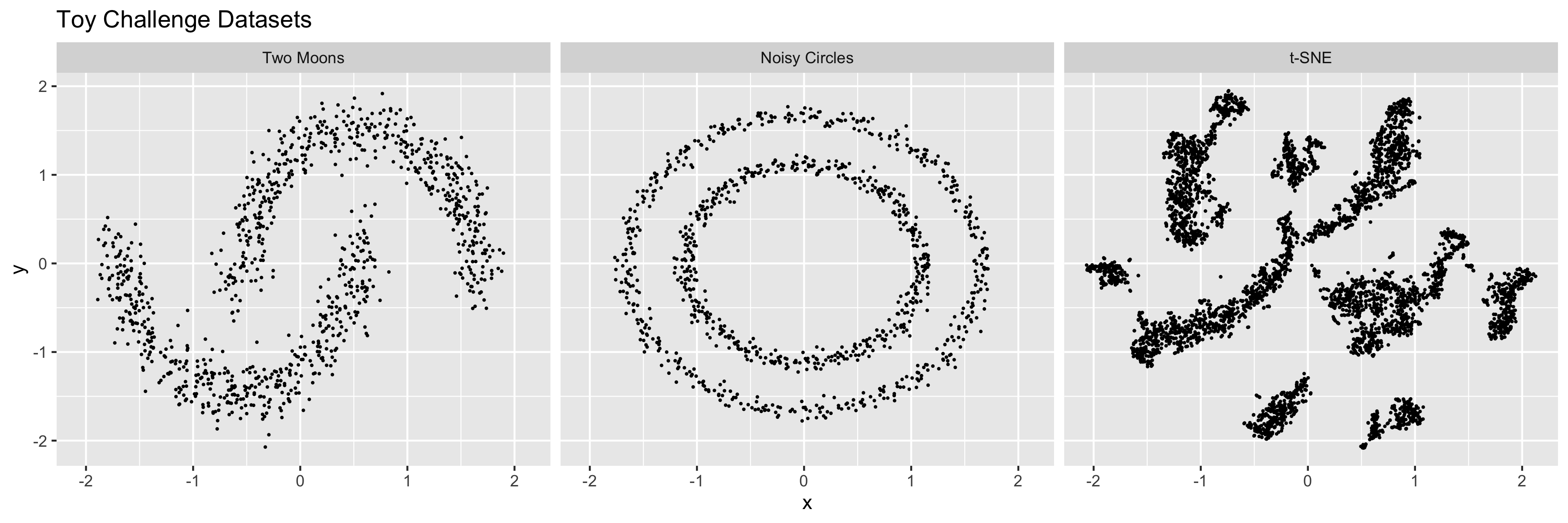
Figure S2: Plots of the toy challenge datasets.

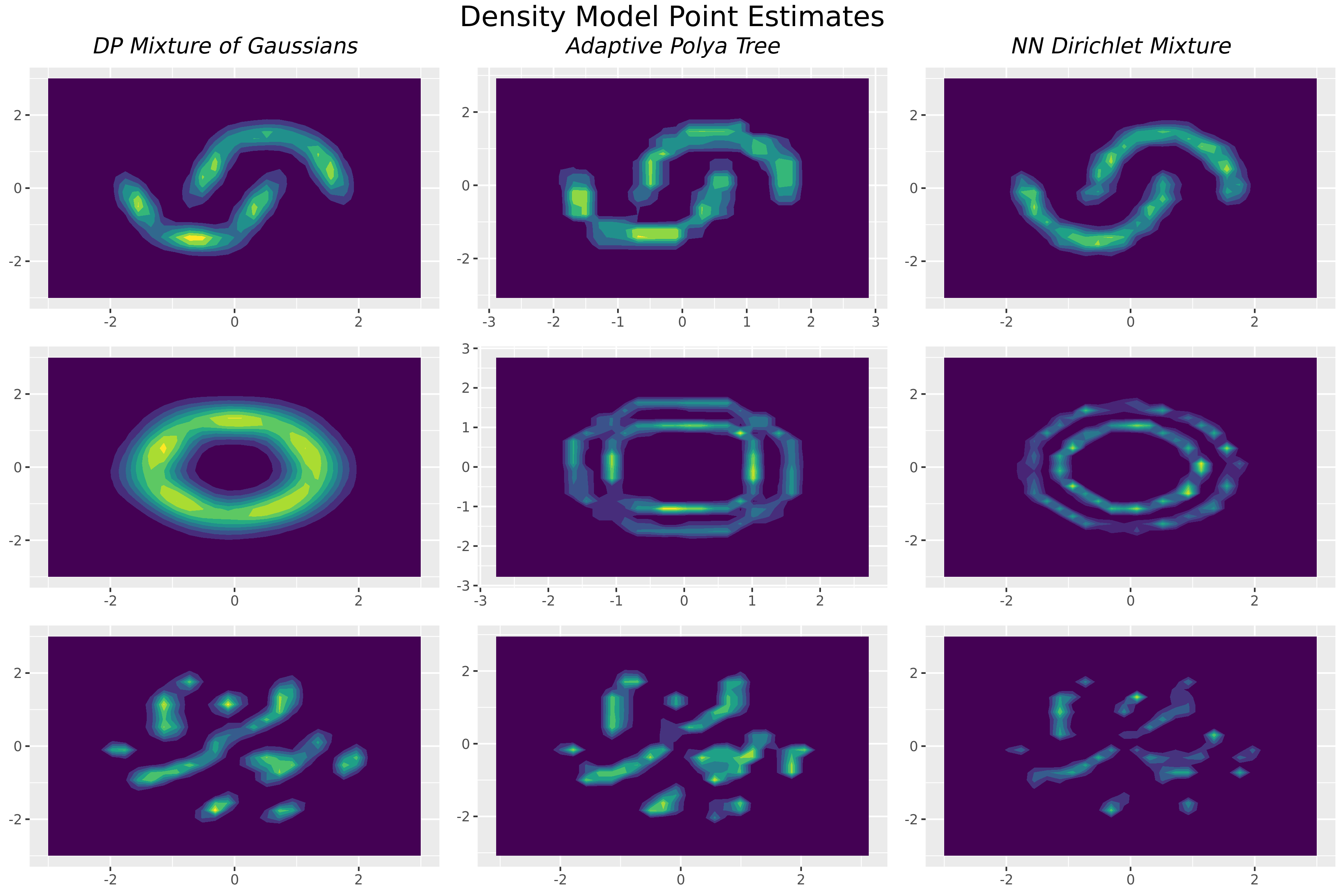
Figure S3: Plots of the toy challenge datasets.

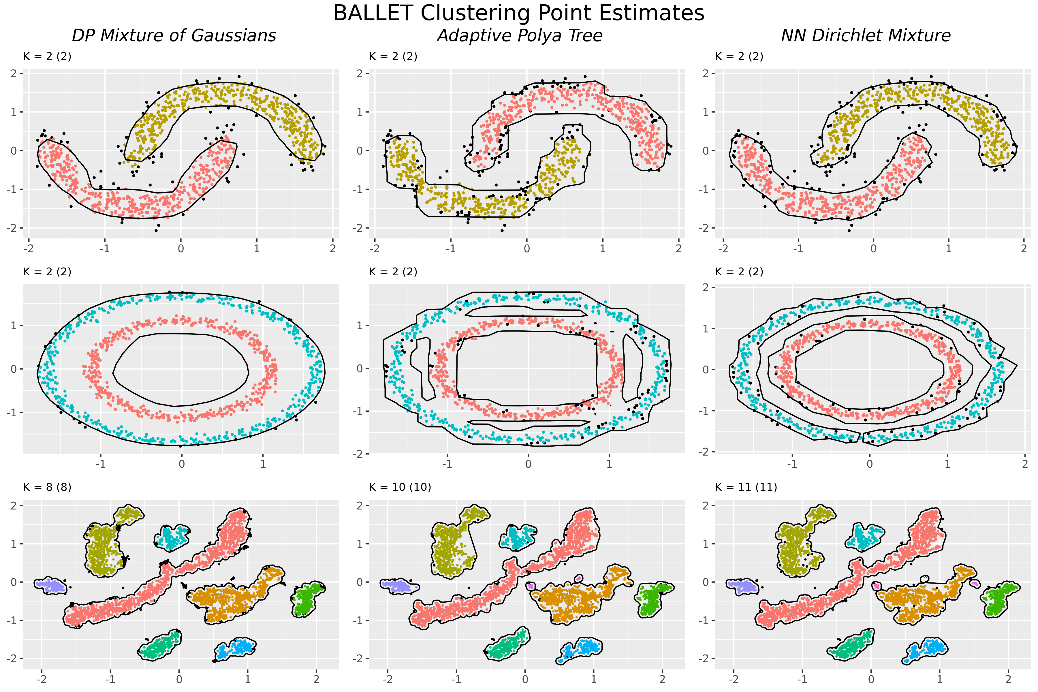
Figure S4: Comparison of BALLET clustering point estimates obtained under the three different density models shown in Figure S3. The cardinality of the partition is displayed in the title of each plot, as $K=X$, and it is followed, in parentheses by the count of clusters with more than 1 observation.

Appendix S5 The mixture of histograms model for densities

This section describes the mixture of histograms model that we use to estimate the data generating density in Section 6. This model can quickly be fit to a large number of data points since the fitting is primarily based on counting the number of observed data points that fall into various bins. Further, in contrast to a standard histogram model, the density function from a mixture of histograms tend to be more regular (smaller jumps).

Let us introduce notation to describe our model. Suppose $X_{i}$ for $i=1,\dots,n$ are independent draws from an unknown distribution with density $f$ supported on a compact set $\mathcal{X}\subseteq\mathbb{R}^{2}$. We assume that $f$ can be represented as a finite mixture $f(x;\bm{\pi},\bm{\mathcal{B}},\bm{\rho})=\sum_{k=1}^{K}\pi_{k}H_{k}(x;\mathcal{B}_{k},\bm{\rho}_{k})$ of $K\in\mathbb{N}$ histogram densities, where $\bm{\pi}=(\pi_{1},\ldots,\pi_{K})$ is a vector of non-negative weights whose coordinates sum to one. For a given $k\in[K]$, the histogram density $H_{k}(x;\mathcal{B}_{k},\bm{\rho}_{k})=\sum_{m=1}^{M}\mathds{1}_{\left[x\in B_{km}\right]}\rho_{km}$ is a step-function based on a partition $\mathcal{B}_{k}=\{B_{k1},\dots,B_{kM}\}$ of size $M$ of $\mathcal{X}$ and a set of associated density values $\bm{\rho}_{k}=(\rho_{km})_{m=1}^{M}$. For simplicity, we fix $|\mathcal{B}_{k}|=M$ for all $k=1,\ldots,K$.

It is convenient to view this model in terms of an equivalent augmented-data representation, associating a latent variable $Z_{i}$ with each observation $X_{i}$, so that $f(x_{i};z_{i},\bm{\mathcal{B}},\bm{\rho})=\sum_{k=1}^{K}\mathds{1}_{\left[z_{i}=k\right]}H_{k}(x_{i};\mathcal{B}_{k},\bm{\rho}_{k})$ and $z_{i}|\bm{\pi}\sim\sum_{k=1}^{K}\pi_{k}\delta_{k}$. We denote the complete set of observations as $\mathcal{D}=\{X_{1},\dots,X_{N}\}$ and the latent histogram allocation variables as $\mathcal{Z}=\{Z_{1},\dots,Z_{N}\}$.

For simplicity, we also assume that $\mathcal{X}=[a,b]\times[c,d]$ and $\mathcal{B}_{k}$ is a grid (or product) based partition of $\mathcal{X}$. More precisely, we assume that there is a partition $\mathcal{U}_{k}=\{U_{k1},\dots,U_{kM^{\prime}}\}$ of $[a,b]$ and $\mathcal{V}_{k}=\{V_{k1},\dots,V_{kM^{\prime}}\}$ of $[c,d]$ so that $\mathcal{B}_{k}=\{U\times V|U\in\mathcal{U}_{k},B\in\mathcal{V}_{k}\}$ and $M=M^{\prime 2}$. We further assume that partitions $\mathcal{U}_{k}$, $\mathcal{V}_{k}$ are constructed based on grid points $\bm{u}_{k}=\{u_{k0},\dots,u_{kM^{\prime}}\}$, $\bm{v}_{k}=\{v_{k0},\dots,v_{kM^{\prime}}\}$ such that $U_{k1}=[u_{k0},u_{k1}]$, $V_{k1}=[v_{k0},v_{k1}]$ and $U_{km}=(u_{k,m-1},u_{k,m}]$ and $V_{km}=(v_{k,m-1},v_{k,m}]$ for $2<m\leq M^{\prime}$.

S5.1 Prior distribution on parameters

We now describe our prior distribution for the parameters of the mixture of histograms model. Focusing first on the partition $\mathcal{B}_{k}$, denote $u_{km}=a+(b-a)\sum_{j=1}^{m}\tilde{u}_{kj}$ and $v_{km}=c+(d-c)\sum_{j=1}^{m}\tilde{v}_{kj}$ so that $\widetilde{\bm{u}}_{k}=(\tilde{u}_{k1},\ldots,\tilde{u}_{kM^{\prime}})$ and $\widetilde{\bm{v}}_{k}=(\tilde{v}_{k1},\ldots,\tilde{v}_{kM^{\prime}})$ lie on the probability simplex. We specify our prior on $\mathcal{U}_{k}$ and $\mathcal{V}_{k}$ (and thus $\mathcal{B}_{k}$) by assuming that $\widetilde{\bm{u}}_{k}\sim\text{Dirichlet}(\alpha_{b}1_{m})$ and $\widetilde{\bm{v}}_{k}\sim\text{Dirichlet}(\alpha_{b}1_{m})$ are independent. The parameters $M^{\prime}$ and $\alpha_{b}$ can be thought of as controlling the bin resolution and regularity for the histograms, respectively. In our sky survey analysis we set $M^{\prime}=50$ ($M=2500$) and $\alpha_{b}=5$.

After specifying our prior for $\mathcal{B}_{k}$, we complete our prior specification for the histogram $H_{k}$ by describing our prior for $\bm{\rho}_{k}$ given $\mathcal{B}_{k}$. Since $H_{k}$ is a density that integrates to one, $\bm{\rho}_{k}$ should satisfy the constraint $\sum_{m=1}^{M}\rho_{km}A_{km}=1$ where $A_{km}$ denotes the Lebesgue measure of bin $B_{km}$. Thus, rather than directly placing a prior on $\bm{\rho}_{k}$, we place a Dirichlet prior on the parameter $\bm{p}_{k}=(p_{k1},\ldots,p_{kM})$, where $p_{km}=A_{km}\rho_{km}$ denotes the probability mass assigned to bin $B_{km}$ by the histogram $H_{k}(x)$. Thus we suppose $\bm{p}_{k}|\mathcal{B}_{k}\sim\text{Dirichlet}(\alpha_{d}\frac{A_{k1}}{A},\dots,\alpha_{d}\frac{A_{kM}}{A})$, choosing $\alpha_{d}=1$ as a default.

Finally, we complete our prior specification on the mixture of histograms model for the unknown density $f$ by choosing to treat all parameters $\{\{\mathcal{B}_{1},\bm{\rho}_{1}\},\dots,\{\mathcal{B}_{K},\bm{\rho}_{K}\}\}$ of the $K$ histograms as a priori independent and fixing the weights $\bm{\pi}=\{\frac{1}{K},\dots,\frac{1}{K}\}$. In our sky survey analysis we set $K=50$.

S5.2 Fast posterior sampling by clipping dependence

We are interested in quickly sampling from the posterior distribution of the density $f\,|\,\mathcal{D}$ when the number of observations $n$ is large. Typically, one would draw samples from the joint posterior $\{\{\mathcal{B}_{1},\bm{\rho}_{1}\},\dots,\{\mathcal{B}_{K},\bm{\rho}_{K}\}\},\mathcal{Z}\,|\,\mathcal{D}$, and then, marginalizing over the uncertainty in $\mathcal{Z}$, use the samples of the histogram parameters to construct a posterior on $f$. An MCMC algorithm designed to converge to this high-dimensional joint posterior object would be extremely computationally intensive, especially given our large sample size, and would likely require an unacceptably large number of samples to converge. Hence, we simplify inferences via a modular Bayes approach similar to that in (liu2009modularization).

Specifically, to update $\bm{\mathcal{B}}$, we sample from its prior distribution rather than its conditional distribution given the data and other parameters, effectively clipping the dependence of the bin parameters on the other components of the model as described in (liu2009modularization). Furthermore, we draw only one sample $\bm{\mathcal{B}}^{*}=\{\mathcal{B}^{*}_{1},\dots,\mathcal{B}^{*}_{K}\}$ from the prior distribution on $\bm{\mathcal{B}}$, and reuse this same collection $\bm{\mathcal{B}}^{*}$ of histogram bins for each round of new samples for the other parameters.

In addition, rather than iterate between sampling $\bm{p}_{k}$ from its full conditional,

$$\bm{p}_{k}|\mathcal{D},\mathcal{Z},\mathcal{B}^{*}_{k}\sim\text{Dirichlet}(\sum_{i=1}^{N}\mathds{1}_{\left[X_{i}\in B_{k1}\right]}\mathds{1}_{\left[Z_{i}=k\right]}+\alpha_{d}\frac{A_{k1}}{A},\dots,\sum_{i=1}^{N}\mathds{1}_{\left[X_{i}\in B_{kM}\right]}\mathds{1}_{\left[Z_{i}=k\right]}+\alpha_{d}\frac{A_{kM}}{A}),$$

and alternately sampling $\mathcal{Z}$ from its full conditional, we marginalize the log density of $\bm{p}_{k}|\mathcal{D},\mathcal{Z},\mathcal{B}^{*}_{k}$ with respect to the prior distribution on $\mathcal{Z}$ yielding the distribution

$$\bm{p}_{k}|\mathcal{D},\mathcal{B}^{*}_{k}\sim\text{Dirichlet}(\frac{N_{k1}}{K}+\alpha_{d}\frac{A_{k1}}{A},\dots,\frac{N_{kM}}{K}+\alpha_{d}\frac{A_{kM}}{A}),$$ (S9)

which we use in place of the posterior distribution of $\bm{p}_{k}$ given $\mathcal{B}^{*}_{k}$ and $\mathcal{D}$. Here $N_{km}=\sum_{i=1}^{N}\mathds{1}_{\left[x_{i}\in B^{*}_{km}\right]}$ denotes the number of observations that fall into the bin $B^{*}_{km}\in\mathcal{B}^{*}_{k}$.

The resulting algorithm is a fast way to generate independent samples from an approximate modular posterior for $f(\mathcal{D})$ without using MCMC. This sampler runs almost instantaneously on a personal laptop computer even for sample sizes of $n\approx 40,000$, which would be prohibitive for traditional MCMC algorithms for posterior computation in density estimation models. Moreover, the samples appear to appropriately reflect our uncertainty in the underlying data-generating density in our experiments.

Appendix S6 Additional results from the analysis of the synthetic sky survey data

Including a diversity of sizes among the synthetic galaxy clusters led to datasets which more closely resembled the observed data, and it also made the true clusters more challenging to recover with both clustering methods. Hence, we simulated the weights of the active components from a symmetric Dirichlet distribution with small concentration parameter. The relative weights of the “galaxy clusters” for one of the 100 synthetic datasets we analyzed are visualized in Figure S5. The specific synthetic dataset associated with these weights is shown in Figure S6.

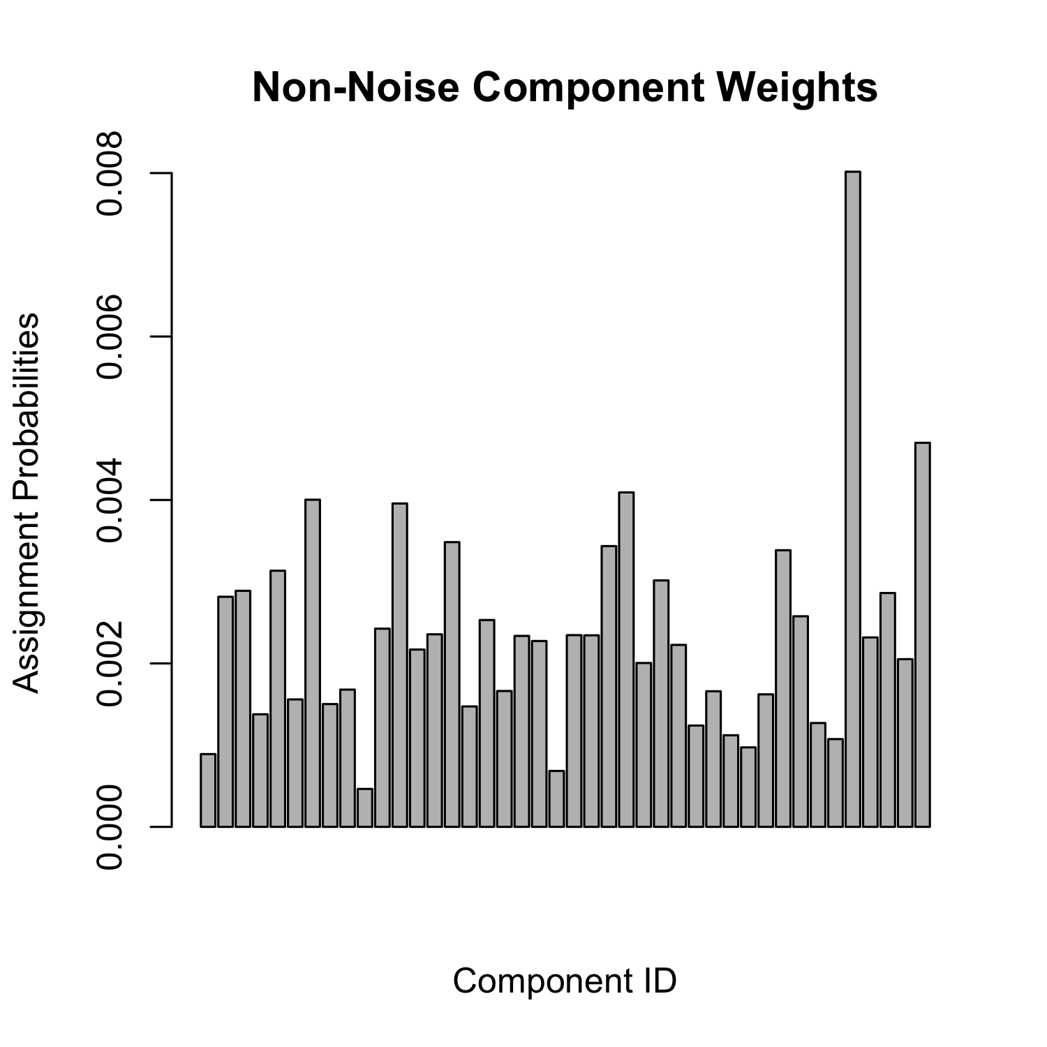
Figure S5: Relative sizes (mixtures weights) of the non-noise components in one of our synthetic sky survey datasets.

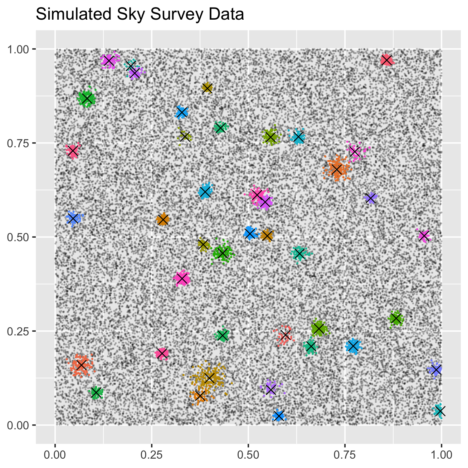
Figure S6: One of our synthetic sky survey datasets. Observations drawn from one of the high-density components are given bright colors, and each of their centers is marked with an $\times$. Observations drawn from the uniform background are colored grey and made translucent.

Figure S8 shows how the performance of DBSCAN is highly sensitive to the choice of tuning parameter. It is interesting to note that the optimal parameters in this application are far from the values suggested by the heuristics proposed in (schubert2017dbscan), suggesting that in general they will be highly context dependent. We show the performance of the optimally tuned DBSCAN in figure S9, noting that this tuning procedure required knowledge of the ground truth. The bounds of the 95% credible ball of the BALLET point estimate for the synthetic data are shown in Figure S10. The associated BALLET point estimate is shown in Figure 4 of the main document. The complete results of the sensitivity and specificity of the various point estimates and bounds considered, averaged over the 100 synthetic datasets, are presented in Table S1.

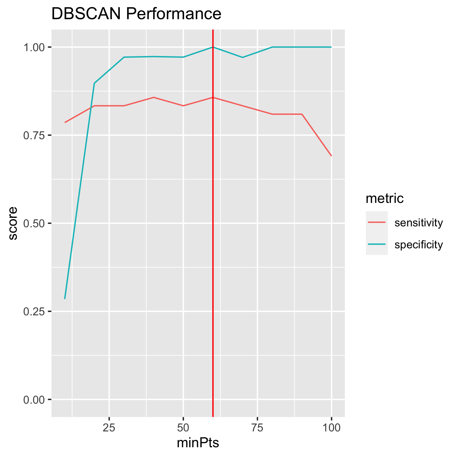
(a) DBSCAN performance vs MinPts tuning parameter

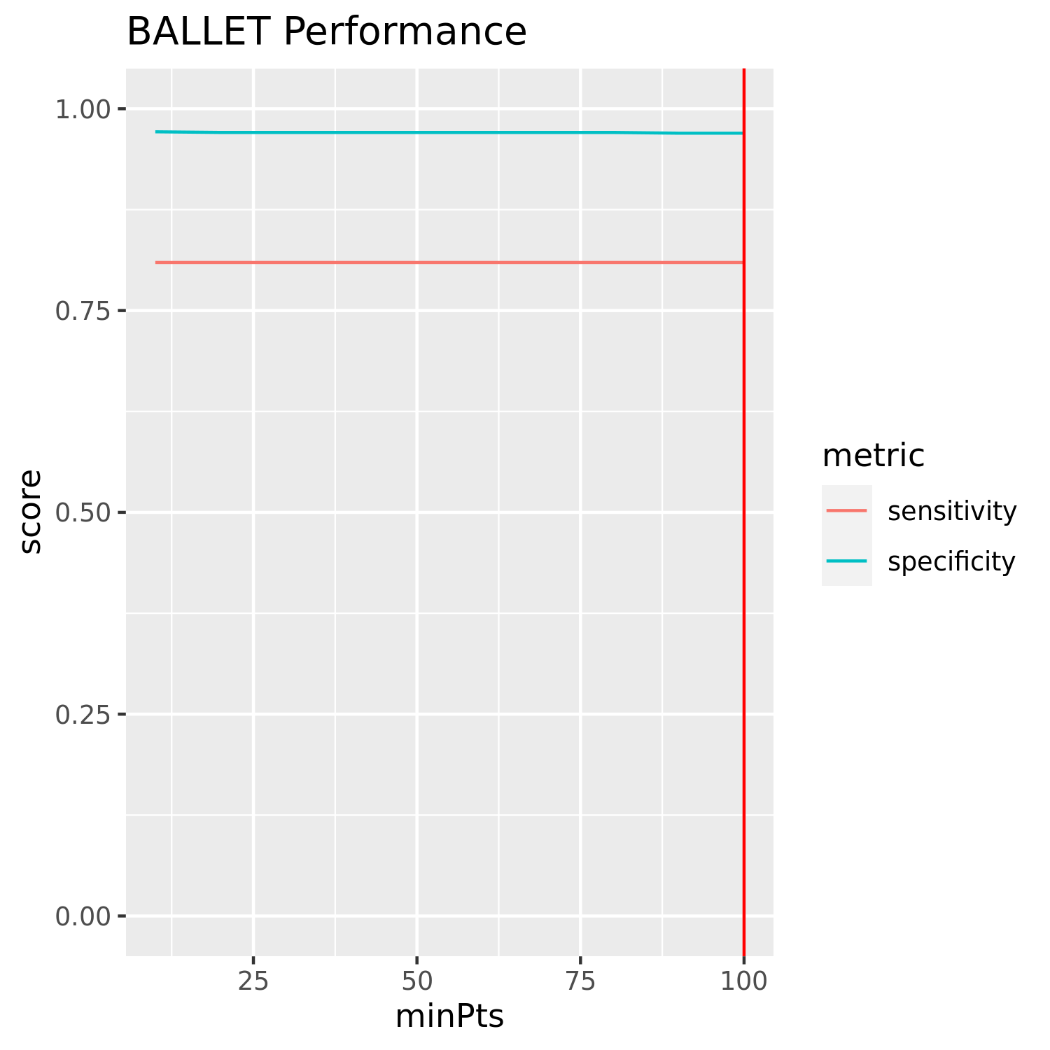
(b) BALLET performance vs MinPts tuning parameter

Figure S8: The performance of BALLET and DBSCAN clusters as the tuning parameter $k$ (or equivalently $\texttt{MinPts}=k+1$) varies. Vertical lines call attention to the value of $k$ that exhibits the “best” performance, as determined by the sum of the sensitivity and specificity.

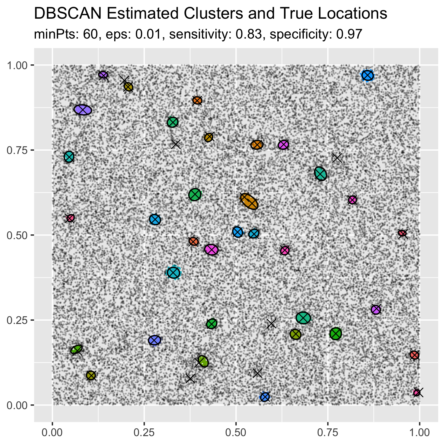
Figure S9: The results of fitting DBSCAN to the particular synthetic sky survey data using the value of tuning parameter MinPts which optimize its observed performance for this dataset.

	DBSCAN	DBSCAN1	BALLET Lower	BALLET Est.	BALLET Upper
Sensitivity	0.86	0.79	0.62	0.79	0.89
Specificity	0.47	0.99	0.99	0.99	0.97
Exact Match	0.43	0.88	0.90	0.87	0.83

Table S1: Averaged results from applying BALLET and DBSCAN to 100 replicates of the synthetic sky survey data. For BALLET, we also provide the performance of upper and lower bounds for a 95% credible ball centered at the point estimate. For DBSCAN, we provide averaged sensitivity and specificity for both the heuristically selected tuning parameters and the optimal tuning parameters.

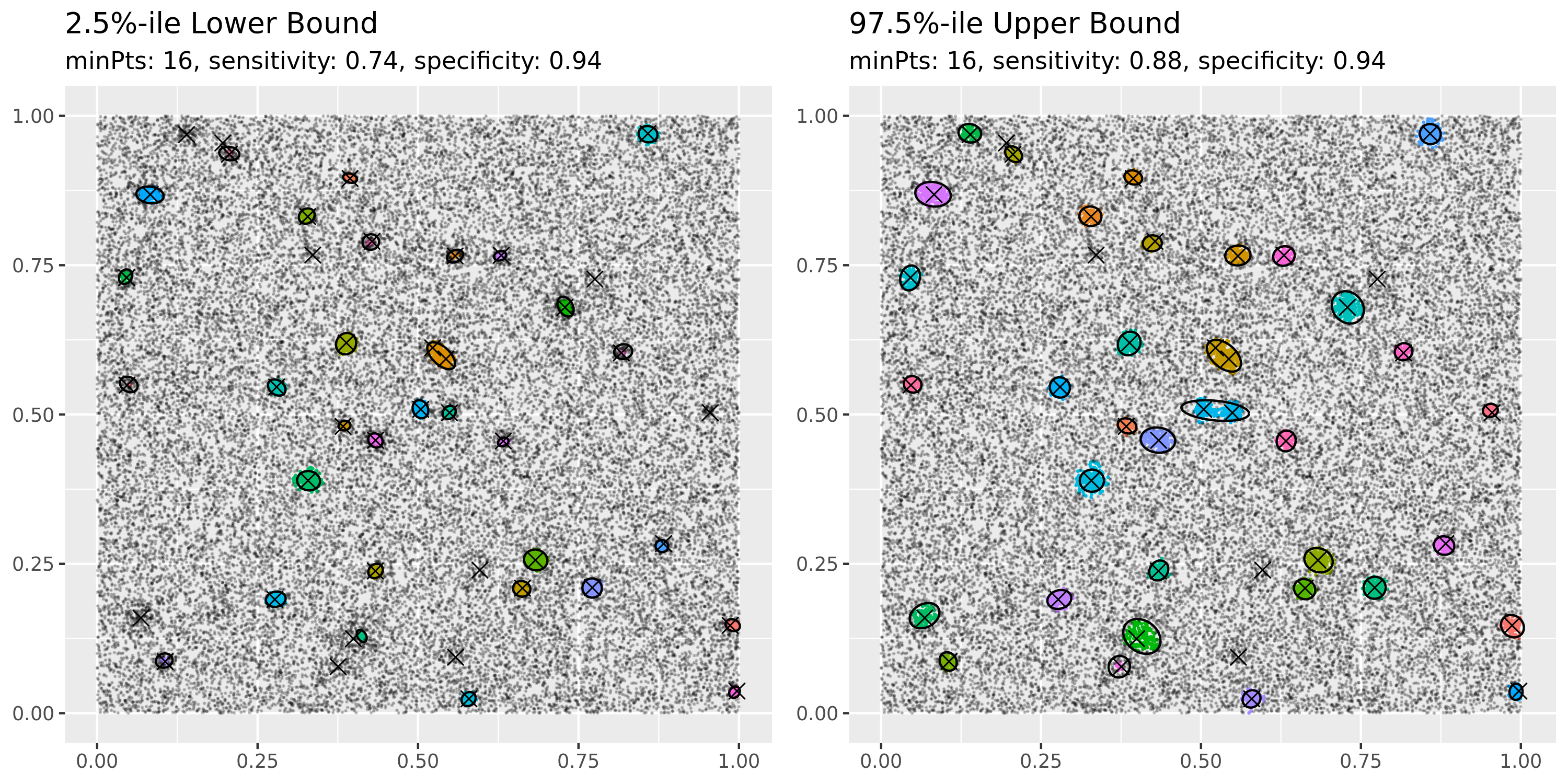
Figure S10: Upper and lower bounds for the 95% credible ball centered at our BALLET clustering estimate for the particular synthetic dataset shown in in Figure S6.

Appendix S7 Additional results from analysis of EDSGC sky survey data

In this section we provide additional results from the analysis of the EDSGC sky survey data which appeared in Section 6 of the main text. In particular, we visualize the log of the posterior expectation of the data generating density in Figure S11, upper and lower bounds for our BALLET clustering analysis in Figure 5, and an alternative DBSCAN fit using the optimal tuning parameters from the simulation study in Figure S14. We present tabular results collecting the rate of coverage of the EDCCI and Abell catalogs, by the various point estimates and bounds we have considered, in Tables 1 and S2, respectively.

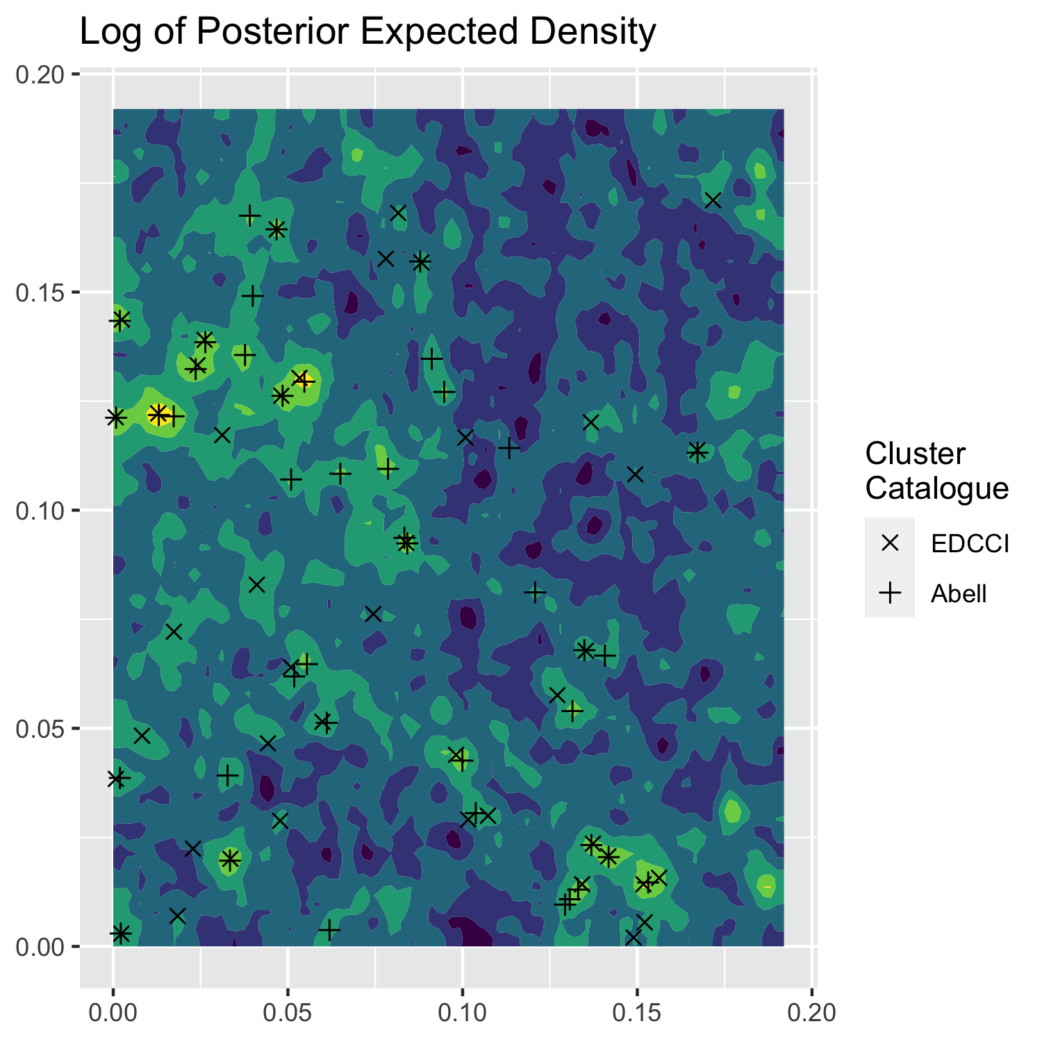
Figure S11: Log of the posterior expectation of the density for the EDSGC data under our mixture of random histograms model. For reference, we have superimposed galaxy clusters reported in the EDCCI and Abell cluster catalogs.

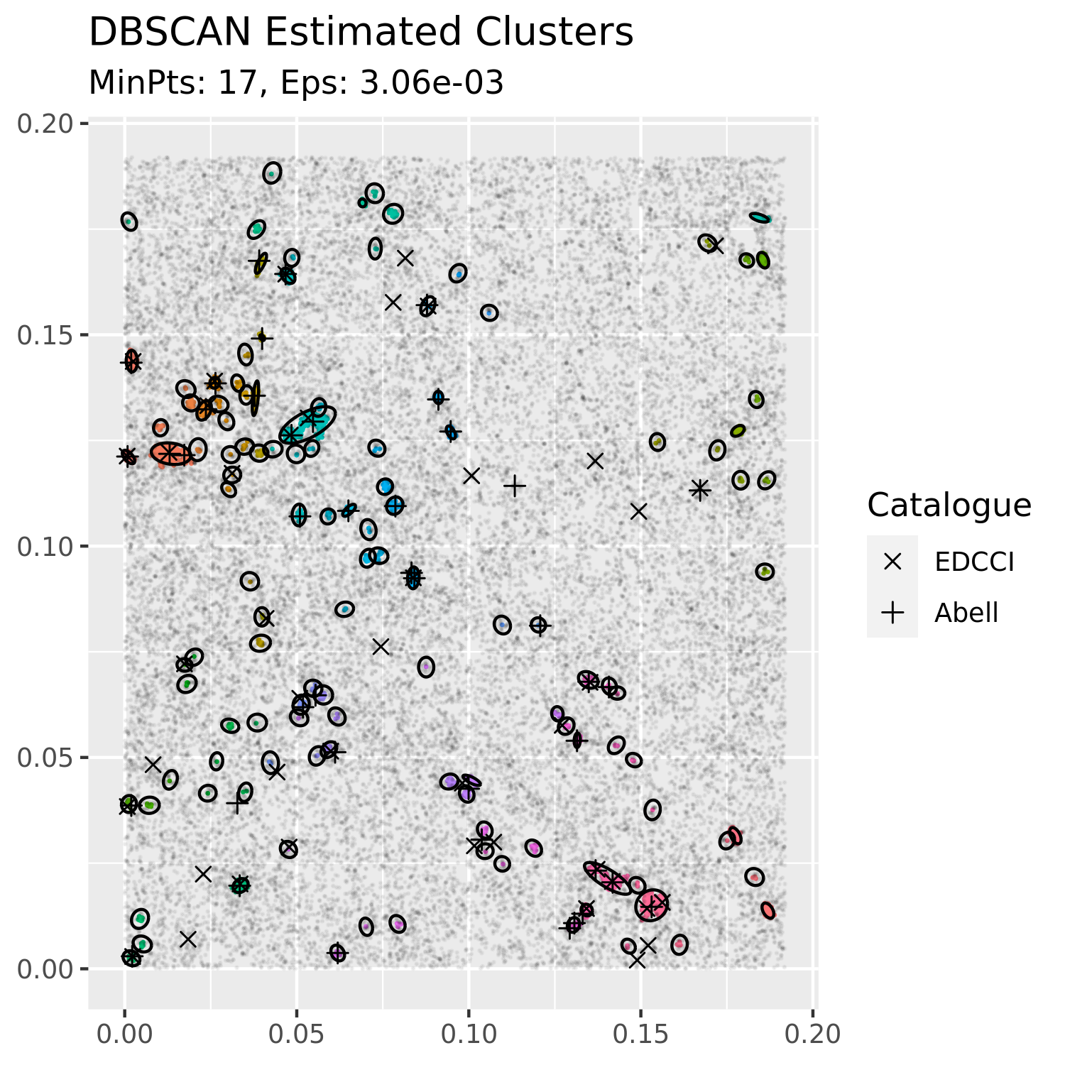
Figure S12: Results of applying DBSCAN to the EDSGC Data, using heuristically selected tuning parameters. Cluster centers from the two previously proposed cluster catalogs are plotted with black ‘+’s (Abell Catalog) and ‘X’s (EDCCI).

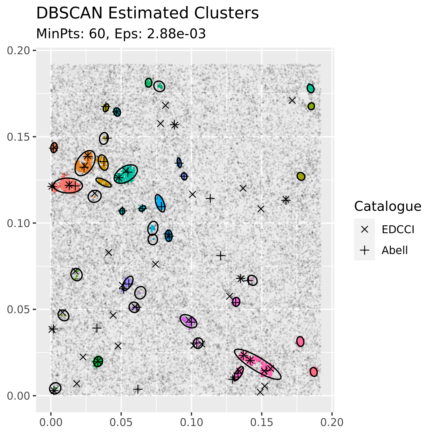
Figure S14: The results of DBSCAN fit to the data using tuning parameters selected based on our calibration to ground truth described in Section S6 rather than based on heuristics recommended in the density-based clustering literature.

Method	Sensitivity (Abell)	Specificity (Abell)	Exact Match (Abell)
DBSCAN	0.40	0.18	0.16
DBSCAN1	0.37	0.42	0.34
BALLET Lower	0.21	0.73	0.67
BALLET Est.	0.40	0.40	0.26
BALLET Upper	0.56	0.34	0.27

Table S2: DBSCAN and BALLET Clustering coverage of the suspected galaxy clusters listed in the Abell catalog. The row labeled “DBSCAN” reports the performance of the method with the standard, heuristically-chosen values of the tuning parameters, while “DBSCAN¹” shows the performance of the method with the optimal value of MinPts chosen based on consideration of the ground truth in our simulation study.

Appendix S8 On the choice of the level $\lambda$

A key problem with level-set clustering is that we may not exactly know the level (campello2020density) or, worse yet, that our results can be sensitive to the exact level that we choose for our analysis. Here we describe how to summarize clustering results across multiple values of the level by visualizing a cluster tree (clustree), and reduce our sensitivity to any single choice of the level by identifying clusters that remain active or “persistent” across all the levels in the tree.

As described in Section 7, we expect the level-set clusters of our EDSGC sky survey data to be sensitive to the exact value of the level $\lambda=(1+c)\bar{f}$, determined by the scientific constant $c$. Since $c$ is believed to be around one (jang2006nonparametric), our preliminary analysis of this data in Section 6 proceeded with the assumption that $\lambda=2\bar{f}$, or equivalently that $c=1$. Here we summarize our results from computing the BALLET clusters at various density levels corresponding to the values $c\in\{.8,.9,\ldots,1.2\}$.

S8.1 Visualizing the cluster tree

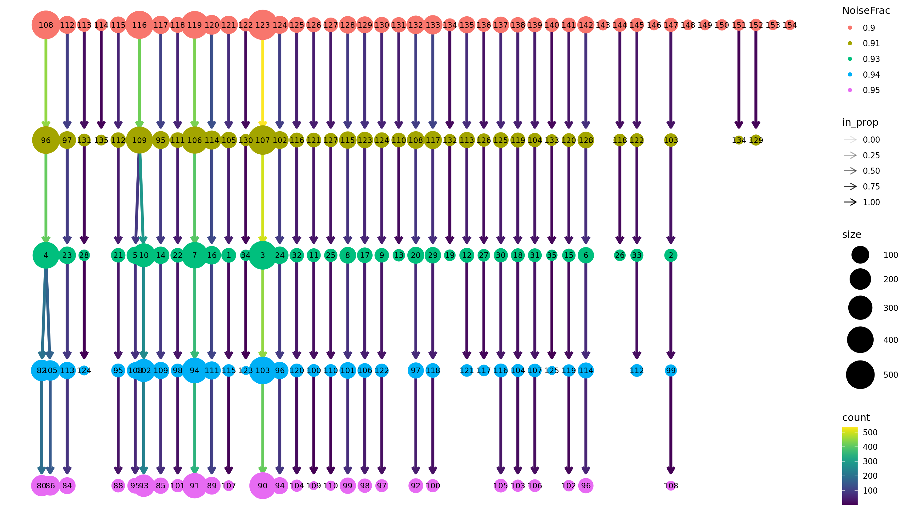
Figure S15: The BALLET cluster tree (clustree) for the Sky Survey data across multiple density levels corresponding to $c\in\{.8,.9,\ldots,1.2\}$. The nodes in each row are the BALLET clusters for the fixed level $\lambda=(1+c)\bar{f}$, where $c$ increases as we go down the tree. An edge between nodes in two successive levels indicates an overlap between the two corresponding clusters. While most clusters at the top level ($c=0.8$) have a unique child in the tree at each lower level (i.e. as $c$ increases), some clusters at the top level split into multiple children or did not have any descendent in the bottom levels. For each cluster at the bottom level, the persistent clustering algorithm finds its topmost ascendant in the tree below any (potential) split.

It is well known (hartigan1975clustering; campello2020density; menardi2016modal) that the level-set clusters across different levels of the same density are nested in a way that can be organized into a tree. In particular, given two clusters from two different levels of the same density, it is the case that either both the clusters are disjoint, or one of the clusters is contained inside the other.

We empirically found that our BALLET estimates across various levels could similarly be organized into a tree. We visualized this tree in Figure S15 by modifying code for the clustree package in R (clustree). We see that while BALLET found 44 clusters at the lower level ($c=.8$), it only found 27 clusters at the higher level ($c=1.2$), indicating that more than a third of the lower level clusters disappear as the choice of the level is slightly increased. Further, in this process, two of the lower level clusters are also seen to split into two clusters each.

S8.2 Persistent Clustering

Given the sensitivity of our level-set clusters to the choice of any single level, we now describe a simple algorithm that processes the cluster tree to extract clusters that are active (persistent) across all the levels in the tree. Note that some clusters can split into multiple sub-clusters as we increase our level in the cluster tree (i.e. go down the tree). In such cases we will only focus on the cluster’s descendants at the time of the last split.

Suppose a cluster tree like Figure S15 is given. Starting from each cluster at the bottom row of the tree, the Persistent Clustering algorithm involves walking up the tree until we (i) either hit the top row of the tree, or (ii) hit a node whose parent has more than one child. The collection of clusters corresponding to the final nodes obtained from these runs will be called persistent clusters.

BALLET persistent clusters for the EDSGC sky survey data are shown in Figure S16. Table S3 compares the performance of BALLET persistent clusters to those at the fixed level ($c=1$). We find that persistent clustering improves specificity on both the Abell and EDCCI catalogs without loss in sensitivity.

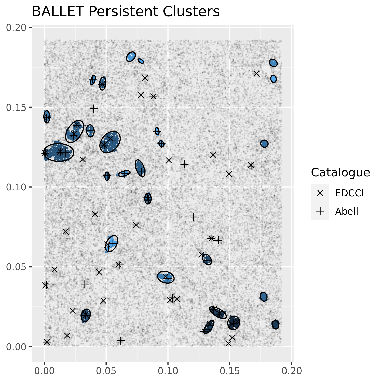
Figure S16: The BALLET persistent clustering estimate for the EDSGC sky survey data across levels $c\in\{.8,\ldots,1.2\}$.

	BALLET (persistent)	BALLET ($c=1$)
Sensitivity (EDCCI)	0.69	0.67
Specificity (EDCCI)	0.74	0.69
Exact Match (EDCCI)	0.48	0.51
Sensitivity (Abell)	0.40	0.40
Specificity (Abell)	0.44	0.40
Exact Match (Abell)	0.26	0.26

Table S3: Comparing results from BALLET persistent clusters across $c\in\{.8,\ldots,1.2\}$ to the BALLET point estimate at $c=1$. Persistent clustering improves the specificity for both the catalogues without losing sensitivity.

.

While we have motivated the idea of persistent clustering by the practical concern of robustness, the idea of obtaining a single flat clustering by cutting the cluster tree at locally adaptive levels has been explored before in the algorithmic level-set clustering literature (mcinnes2017hdbscan; campello2020density). Such methods are useful when we want to recover density-based clusters that can only be separated by considering differing values of the levels (Figure S17).

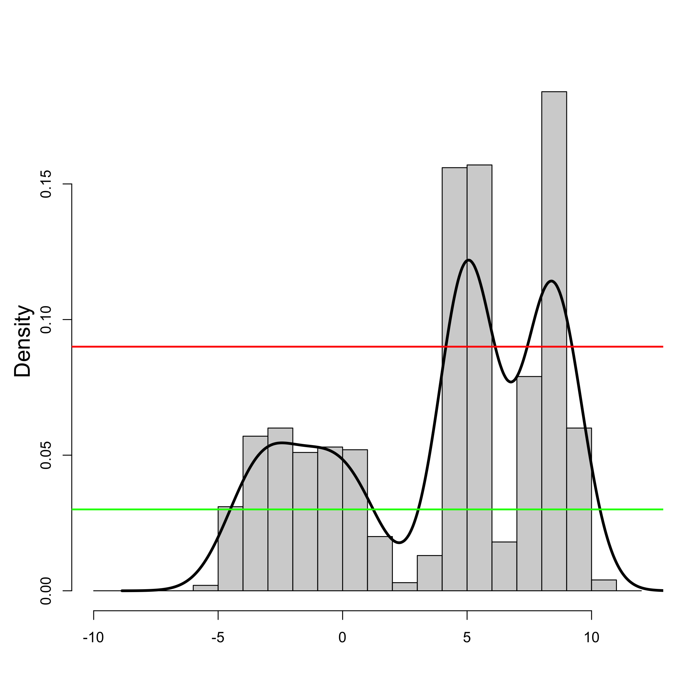
Figure S17: An example of a situation in which we might want to cluster data according to locally adaptive levels.