Almost Global Asymptotic Trajectory Tracking for Fully-Actuated Mechanical Systems on Homogeneous Riemannian Manifolds

Abstract

In this work, we address the design of tracking controllers that drive a mechanical system’s state asymptotically towards a reference trajectory. Motivated by aerospace and robotics applications, we consider fully-actuated systems evolving on the broad class of homogeneous spaces (encompassing all vector spaces, Lie groups, and spheres of any dimension). In this setting, the transitive action of a Lie group on the configuration manifold enables an intrinsic description of the tracking error as an element of the state space, even in the absence of a group structure on the configuration manifold itself (e.g., for $\mathbb{S}^{2}$). Such an error state facilitates the design of a generalized control policy depending smoothly on state and time that drives this geometric tracking error to a designated origin from almost every initial condition, thereby guaranteeing almost global convergence to the reference trajectory. Moreover, the proposed controller simplifies naturally when specialized to a Lie group or the $n$-sphere. In summary, we propose a unified, intrinsic controller guaranteeing almost global asymptotic trajectory tracking for fully-actuated mechanical systems evolving on a broader class of manifolds. We apply the method to an axisymmetric satellite and an omnidirectional aerial robot.

I Introduction

An efficient and effective architecture for the control of mechanical systems synthesizes the overall controller as the composition of a low-rate “open-loop” planner (to select a reference trajectory) with a high-rate “closed-loop” tracking controller (to drive the system towards the reference trajectory). Such layered control architectures are found across an extremely diverse array of engineered and biological systems, demonstrating the effectiveness of the paradigm [2].

For some mechanical systems, it is possible to reduce the “tracking problem” to the easier “regulation problem” (i.e., asymptotically stabilizing an equilibrium) for the same system, using a state-valued “tracking error” between the reference and actual states that “vanishes” only when the two are equal (e.g., $({q-q_{d}},{\dot{q}-\dot{q}_{d}})$ for a mechanical system on ${\mathbb{R}^{n}}$). Then, feedback is designed to drive the error towards the origin, i.e., a constant (equilibrium) trajectory. Such a reduction is substantially easier for fully-actuated (vs. underactuated) systems, since arbitrary forces can be exerted to compensate for time variation in the reference and also inject suitable artificial potential and dissipation terms to almost globally asymptotically stabilize the error [3].

Clearly, a smooth tracking controller that is well-defined on the entire state space (in general, the tangent bundle of a non-Euclidean manifold) cannot rely on a local, coordinate-based tracking error. When the configuration manifold is a Lie group, [4] shows that the group structure furnishes an intrinsic, globally-defined tracking error on the state space, via the action of the group on itself. For this reason, [4] remarks that “the tracking problem on a Lie group is more closely related to tracking on $\mathbb{R}^{n}$ than it is to the general Riemannian case, for which the group operation is lacking.”

Tracking via error regulation on manifolds that may not be Lie groups is proposed in [1]. The authors present a theorem ensuring almost global tracking for fully-actuated systems on compact Riemannian manifolds, assuming the control inputs can be chosen to solve a “rank one” underdetermined linear system at each state and time. Solutions exist in some special cases (e.g., on $\mathbb{S}^{2}$ with carefully chosen potential, dissipation, and kinetic energy), although they are non-unique. In other cases, no solutions exist, and the question of when solutions exist in general is left open. Also, the control inputs may not depend continuously on state and time, a desirable property that justifies seeking only almost global stability [5].

In view of these observations, and in pursuit of a systematic approach to tracking control for fully-actuated mechanical systems in yet a broader setting, a question emerges:

On which class of manifolds can the tracking problem be reduced to the regulation problem?

We pose this question in a global or almost global sense; if purely local convergence suffices, the answer is trivial (i.e., “all of them”), since smooth manifolds are locally Euclidean.

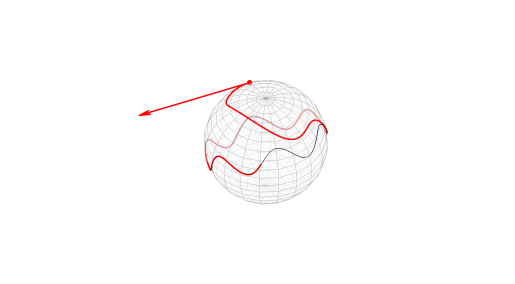
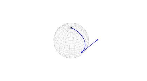
Figure 1: The proposed method, applied to almost global reduced-attitude tracking for the axisymmetric satellite, modeled as a mechanical system on $\mathbb{S}^{2}$ (with state in $T\mathbb{S}^{2}$). As the configuration error (blue) converges to the designated origin (black circle), the actual configuration trajectory (red) converges to the reference (black) . Initial conditions in $T\mathbb{S}^{2}$ for the state and tracking error are shown. The particular gains ${k_{P}=4},{k_{D}=4}$ used here render the linearization of the error dynamics slightly underdamped.

In this work, we consider mechanical systems evolving on homogeneous spaces, a class of manifolds that includes all Lie groups but is more general. In this regime, we obtain globally valid “error dynamics” by extending a tracking error proposed for kinematic systems in [6] to the mechanical setting, exploiting the transitive action of a Lie group on the configuration manifold even when it lacks a group structure of its own. Ultimately, we contribute a systematic approach to tracking control with formal guarantees for a broad class of systems including many space, aerial, and underwater robots.

II Mathematical Background

For any map ${(x,y)\mapsto f(x,y)}$, we define the map ${f_{x}:y\mapsto f(x,y)}$ (resp. ${f^{y}:x\mapsto f(x,y)}$) by holding the first (resp. second) argument constant. For a smooth map ${f:M\to N}$ between manifolds, its derivative is denoted ${\operatorname{d}f:TM\to TN}$, while the dual of its derivative is the unique map ${\operatorname{d}f^{*}:T^{*}M\to T^{*}N}$ such that ${\big{\langle}{\hskip 1.0pt}\omega{\hskip 1.5pt;\hskip 1.5pt}\operatorname{d}f(X){\hskip 1.0pt}\big{\rangle}=\big{\langle}{\hskip 1.0pt}\operatorname{d}f^{*}(\omega){\hskip 1.5pt;\hskip 1.5pt}X{\hskip 1.0pt}\big{\rangle}}$ for any covector field ${\omega\in\Gamma(T^{*}N)}$ and any vector field ${X\in\Gamma(TM)}$. The derivative of any function ${V:M\to\mathbb{R}}$ induces a covector field ${\operatorname{d}V:M\to T^{*}M}$. We assume all curves to be smooth.

II-A Homogeneous Riemannian Manifolds

Definition 1 (see [7, Ch. 3]).

A homogeneous Riemannian manifold $(Q,\Phi,\kappa)$ is a smooth manifold $Q$ equipped with:

1. a transitive action $\Phi:G\times Q\to Q$ of a Lie group $G$, i.e., ${\forall\ q_{1},q_{2}\in Q}$, ${\exists\ g\in G\textrm{ s.t. }\Phi(g,q_{1})=q_{2}}$, and

2. a $\Phi$-invariant Riemannian metric $\kappa$, i.e., ${\forall\ g\in G}$ and ${v_{q},w_{q}\in TQ},\ \kappa\big{(}{v_{q}},{w_{q}}\big{)}=\kappa\big{(}{\operatorname{d}\Phi_{g}(v_{q}),\operatorname{d}\Phi_{g}(\omega_{q})}\big{)}$.

For each ${q\in Q}$, its stabilizer is the maximal subgroup $G_{q}$ of $G$ such that ${\forall\ g\in G_{q},\ \Phi(g,q)=q}$. ${\mathds{1}\in G}$ is the identity.

Example 1 (name=The $n$-Sphere,label=example:sphere).

For any ${n\in\mathbb{N}}$, consider the sphere $\mathbb{S}^{n}$ and the rotation group ${SO(n+1)}$. For notational convenience, we model these manifolds as an embedded submanifolds of Euclidean spaces, i.e., we let ${\mathbb{S}^{n}=\{s\in\mathbb{R}^{n+1}:s^{\textrm{T}}s=1\}}$ and we let ${SO(n+1)=}$ ${\{R\in\mathbb{R}^{n+1\times n+1}:R^{\textrm{T}}R=R\,R^{\textrm{T}}=\mathds{1},\ \det R=1\}}$. Let $\rho$ and $\Psi$ be the respective restriction to ${\mathbb{S}^{n}\subset\mathbb{R}^{n+1}}$ of the Euclidean metric and the usual action of ${SO(n+1)}$, i.e.,

$$\begin{gathered}{\Psi}:SO(n+1)\times\mathbb{S}^{n}\to\mathbb{S}^{n},\ (R,q)\mapsto R\,q.\end{gathered}$$ (1)

Then, it can be shown that $(\mathbb{S}^{n},\Psi,\rho)$ is an ${SO(n+1)}$-homogeneous Riemannian manifold. Moreover, $\rho$ induces the canonical isomorphisms ${\rho^{\flat}:T\mathbb{S}^{n}\to T^{*}\mathbb{S}^{n},v_{q}\to v_{q}{}^{\textrm{T}}\textrm{ and}}$ ${\rho^{\sharp}:T^{*}\mathbb{S}^{n}\to T\mathbb{S}^{n},f_{q}\to f_{q}{}^{\textrm{T}}}$, and ${G_{q}\cong SO(n)}\ \forall\ {q\in\mathbb{S}^{n}}$.

Example 2 (name=A Lie Group,label=example:group).

Consider any Lie group $G$, the left action of $G$ on itself (i.e., ${L:(h,g)\mapsto hg}$), and any $L$-invariant metric $\kappa_{\mathbb{I}}$. Then by [8, Thm. 5.38] there exists an inner product $\mathbb{I}$ on ${\mathfrak{g}\cong T_{\mathds{1}}G}$ such that ${\forall\ v_{g},w_{g}\in TG}$,

$$\kappa_{\mathbb{I}}(v_{g},w_{g})=\mathbb{I}\,\big{(}\operatorname{d}L_{g^{-1}}(v_{g}),\operatorname{d}L_{g^{-1}}(w_{g})\big{)}.$$ (2)

Moreover, $(G,L,\kappa_{\mathbb{I}})$ is a $G$-homogeneous Riemannian manifold. The action $L$ is free, i.e., for ${g\neq\mathds{1}}$, the map $L_{g}$ has no fixed points. Thus, the stabilizer of ${g\in G}$ is just ${G_{g}=\{\mathds{1}\}}$. It is clear that for all ${\xi\in\mathfrak{g}}$ and ${\tau\in\mathfrak{g}^{*}}$, we have ${\kappa_{\mathbb{I}}^{\flat}(\xi)=\mathbb{I}^{\flat}(\xi)}$ and ${\kappa_{\mathbb{I}}^{\sharp}(\tau)=\mathbb{I}^{\sharp}(\tau)}$ (see, e.g., [8, Sec. 2.3.4]).

II-B Navigation Functions

The following functions are described in [3] (in the more general setting of manifolds with boundary). They are useful in generating artificial potential forces for stabilization.

Definition 2.

On a boundaryless manifold $Q$ with origin ${0_{Q}\in Q}$, a $0_{Q}$-navigation function is a proper Morse function ${P:Q\to\mathbb{R}}$ with $0_{Q}$ as its unique local minimizer. A given navigation function is perfect if its domain admits no other navigation function with fewer critical points.

For example, for any ${0_{\mathbb{S}^{n}}\in\mathbb{S}^{n}}$ and $k_{P}>0$, the map

$$P_{\mathbb{S}^{n}}:\mathbb{S}^{n}\to\mathbb{R},\ q\mapsto-k_{P}\,({0_{\mathbb{S}^{n}}})^{\textrm{T}}\,q$$ (3)

is a ${0_{\mathbb{S}^{n}}}$-navigation function. Following [3], a perfect $\mathds{1}\textrm{-navigation}$ function on ${SE(3)\subset GL_{4}(\mathbb{R})}$ can be given by

$$P_{SE(3)}:\begin{pmatrix}R&x\\ 0_{1\times 3}&1\end{pmatrix}\mapsto\operatorname{tr}\big{(}K_{R}(\mathds{1}-R)\big{)}+x^{\mathrm{T}}K_{x}\,x,$$ (4)

where ${R\in SO(3)}$, ${x\in\mathbb{R}^{3}}$, and $K_{R},K_{x}$ are $3\times 3$ symmetric positive-definite matrices and $K_{R}$ has distinct eigenvalues. The restriction of $P_{SE(3)}$ to any closed subgroup of $SE(3)$ is a navigation function on that subgroup, and a navigation function on the product of boundaryless manifolds can be given by the sum of navigation functions on each factor [9]. Thus, we have an explicit navigation function on the product of any number of $n$-spheres and closed subgroups of $SE(3)$, capturing most configuration manifolds of particular interest.

II-C Almost Global Asymptotic Tracking

Definition 3.

For a control system ${\dot{x}=f(x,u)}$ evolving on a metric space ${(X,\operatorname{dist}_{X})}$, a control policy ${u=u(t,x)}$ achieves almost global asymptotic tracking of a reference trajectory ${x_{d}:\mathbb{R}\to X}$ if, for each ${t_{0}\in\mathbb{R}}$, there exists a residual set ${S_{t_{0}}\subseteq X}$ of full measure such that ${x(t_{0})\in S_{t_{0}}\implies\operatorname{dist}_{X}(x(t),x_{d}(t))\to 0}$ as ${t\to\infty}$.

III An Intrinsic, State-Valued Tracking Error

In this section, we extend a contribution made in [6] (which dealt with kinematic systems) to describe an intrinsic state-valued tracking error suitable for mechanical systems.

III-A Tracking Error in Homogeneous Spaces

Definition 4.

For an origin ${0_{Q}}$ in $(Q,\Phi,\kappa)$ and a smooth curve ${q_{d}:\mathbb{R}\to Q}$, a $0_{Q}$-lift of $q_{d}$ is any smooth curve ${g_{d}:\mathbb{R}\to G}$ such that $\Phi\big{(}g_{d}(t),0_{Q}\big{)}=q_{d}(t)\textrm{ for all }t\in\mathbb{R}.$

Definition 5.

For any actual and reference configuration trajectories ${q,q_{d}:\mathbb{R}\to Q}$ and a given $0_{Q}$-lift $g_{d}$ of $q_{d}$, the configuration error trajectory is the smooth curve given by

$$e:\mathbb{R}\to Q,\ t\mapsto\Phi\big{(}{g_{d}}(t)^{-1},q(t)\big{)},$$ (5)

while the state error trajectory is its derivative, ${\dot{e}:\mathbb{R}\to TQ}$.

In [6], the authors define a tracking error of the form (5) for kinematic (i.e., first-order) systems evolving on homogeneous spaces, which is used to synthesize optimal tracking controllers with local convergence. We lift this definition to the tangent bundle to obtain a state-valued tracking error for mechanical (i.e., second-order) systems. The following proposition extends [6, Prop 4.1] to the second-order setting and justifies the use of the term “tracking error”.

Proposition 1.

Consider any actual and reference trajectories ${q,q_{d}:\mathbb{R}\to Q}$. Let ${g_{d}:\mathbb{R}\to G}$ be a $0_{Q}$-lift of ${q_{d}}$, and let ${0_{TQ}\in TQ}$ be the zero tangent vector at $0_{Q}$. Then, for any time ${t\in\mathbb{R}}$, ${\dot{q}(t)=\dot{q}_{d}(t)}$ if and only if ${\dot{e}(t)=0_{TQ}}$.

Proof.

Suppressing the $t$-dependence, we note that

$$q =\Phi(g_{d},\Phi({g_{d}^{-1}},q))=\Phi({g_{d}},e),\quad q_{d}=\Phi(g_{d},0_{Q}),$$ (6)

since by assumption, $g_{d}$ is a $0_{Q}$-lift of $q_{d}$. Thus, we have

$$\dot{q}=\operatorname{d}\Phi^{e}(\dot{g}_{d}) +\operatorname{d}\Phi_{g_{d}}(\dot{e}),$$ (7a)

$$\dot{q}_{d}=\operatorname{d}\Phi^{0_{Q}}(\dot{g}_{d}) +\operatorname{d}\Phi_{g_{d}}(0_{TQ}).$$ (7b)

Assuming for sufficiency that ${\dot{e}=0_{TQ}}$ (and therefore ${e=0_{Q}}$), (7a)-(7b) immediately implies that ${\dot{q}=\dot{q}_{d}}$. Assuming for necessity that ${\dot{q}=\dot{q}_{d}}$ (and therefore ${q=q_{d}}$), we recall that $\Phi_{g}$ and $\operatorname{d}\Phi_{g}$ are automorphisms of $Q$ and $TQ$ respectively for each ${g\in G}$. Then, (6) and the invertibility of $\Phi_{g_{d}}$ implies that ${e=0_{Q}}$, while in view of that conclusion and (7a)-(7b), the invertibility of $\operatorname{d}\Phi_{g_{d}}$ implies that ${\dot{e}=0_{TQ}}$. ∎

In summary, the intrinsic tracking error smoothly transforms the state space (in a manner depending smoothly on time) in such a way that only the current reference state is mapped to the zero tangent vector over the origin of the lift. Also, for any $\Phi$-invariant distance metric ${\operatorname{dist}_{Q}:Q\times Q\to\mathbb{R}}$ (e.g., the Riemannian distance $\operatorname{dist}_{\kappa}$), (6) implies that ${\operatorname{dist}_{Q}\big{(}q(t),q_{d}(t)\big{)}=\operatorname{dist}_{Q}\big{(}e(t),0_{Q}\big{)}}$. In this sense, the configuration error (5) captures the disparity between the actual and reference configurations “accurately”.

III-B Computing Horizontal Lifts of Curves

The following notions will aid in computing a lift of a given reference trajectory (and ultimately, the tracking error).

Definition 6 (see [10, Sec. 23.4]).

For a homogeneous Riemannian manifold $(Q,\Phi,\kappa)$ with designated origin ${0_{Q}\in Q}$, a reductive decomposition is a splitting ${\mathfrak{g}=\mathfrak{f}\oplus\mathfrak{q}}$, where ${F=\exp\mathfrak{f}\cong G_{0_{Q}}}$ (the stabilizer at $0_{Q}$) and ${\mathfrak{q}\subseteq\mathfrak{g}}$ is an $\operatorname{Ad}_{F}$-invariant subspace (which need not be closed under $[\hskip 0.5pt\cdot\hskip 1.0pt,\cdot\hskip 0.5pt]$).

Lemma 1 (see [11, Sec. 7]).

A reductive decomposition ${\mathfrak{g}=\mathfrak{f}\oplus\mathfrak{q}}$ always exists whenever ${F:=G_{0_{Q}}}$ is compact.

Proposition 2 (Horizontal Lifts in Reductive Homogeneous Spaces).

Consider a $G$-homogeneous Riemannian manifold $(Q,\Phi,\kappa)$ with origin origin ${0_{Q}\in Q}$ and reductive decomposition ${\mathfrak{g}=\mathfrak{f}\oplus\mathfrak{q}}$. For each smooth curve ${q_{d}:\mathbb{R}\to Q}$ and initial point ${g_{0}\in G}$ such that ${\Phi(g_{0},0_{Q})=q_{d}(0)}$, there exists a unique smooth curve ${g_{d}:\mathbb{R}\to G}$ (called the horizontal lift of $q_{d}$ through $g_{0}$) with the following properties:

1. Lifting: ${g_{d}}$ is a $0_{Q}$-lift of $q_{d}$,

2. Initial Condition: $g_{d}(0)=g_{0}$, and

3. Horizontality: $\operatorname{d}L_{g_{d}(t)}^{-1}\big{(}\dot{g}_{d}(t)\big{)}\in\mathfrak{q}\ \forall\ t\in\mathbb{R}$.

Proof.

By [12, Prop 9.33], $G$ is a (left) principal $F$-bundle over ${Q=G/F}$. In particular, the projection map is given by ${\pi:G\to Q,\ g\mapsto\Phi(g,0_{Q})}$, while the free and proper action is given by ${\Upsilon:F\times G\to G,(f,g)\mapsto R_{f^{-1}}(g)}$. Using the $\operatorname{Ad}_{F}$-invariance of $\mathfrak{q}$, it can be shown that ${HG=}$ ${\{\operatorname{d}L_{g}(\mathfrak{q}):g\in G\}}$ is a principal connection on ${\pi:G\to Q}$. Then, the claim follows from the existence and uniqueness of horizontal lifts in principal bundles (see [13, Sec. 2.9]). ∎

Remark 1 (Sections, Lifts, and Nontrivial Bundles).

The proof of Proposition 2 describes a sense in which a lift projects “down” to the original curve via $\pi$. If the principal bundle ${\pi:G\to Q}$ is trivial (i.e., ${G\cong Q\times F}$ globally and not merely locally), then there exist global sections ${\sigma:Q\to G}$, i.e., smooth maps satisfying ${\pi\circ\sigma=\operatorname{id}}$. In fact, any such section furnishes a (perhaps non-horizontal) lift ${g_{d}:t\mapsto\sigma\circ q_{d}(t)}$. However, when ${\pi:G\to Q}$ is a nontrivial bundle (e.g., the bundle corresponding to $(\mathbb{S}^{2},\Psi,\rho)$, namely ${\pi:SO(3)\to\mathbb{S}^{2}}$), the nonexistence of global sections makes it impossible generate global lifts using a section, nor can the initial value $g_{0}$ of a horizontal lift be chosen in a manner depending continuously on $q_{d}(0)$ alone. Thus, when using horizontal lifts to compute the tracking error, continuous deformation of the reference trajectory can result in discontinuous changes in the tracking error. However, such a discontinuity is with respect to the choice of reference trajectory (i.e., the planning layer); once a reference trajectory has been selected, the configuration error depends smoothly on both time and state. It also should be noted that even for a horizontal lift $g_{d}$ of some $q_{d}$, when ${q_{d}(t_{1})=q_{d}(t_{2})}$ it may still be the case that ${g_{d}(t_{1})\neq g_{d}(t_{2})}$ (see [13, Fig. 3.14.2]), due to the nontrivial holonomy induced by the curvature of a generic principal connection. Since flat principal connections do not exist on nontrivial bundles, this cannot be avoided in general; see [13, Ch. 3] for broader discussion of holonomy.

Remark 2 (Computing Horizontal Lifts Numerically).

Let ${(\pi\times\varphi^{i}):}$ ${\pi^{-1}(U_{i})\subseteq G}$ ${\to}$ ${(U_{i}\subseteq Q)\times F,}$ ${i\in\{1,\ldots,k\}}$ be a collection of local trivializations covering ${\pi:G\to Q}$. Let ${\mathbb{A}^{i}:TU_{i}\to\mathfrak{f}}$ be the local connection forms for $HG$ (see [13, Prop. 2.9.12]). Suppose ${q_{d}(t)\in U_{j}}$ for ${t\in[t_{1},t_{2}]}$ and let ${f^{j}:[t_{1},t_{2}]\to F}$ solve the initial value problem (IVP)

$$f^{j}(t_{1})=\varphi^{\hskip 0.75ptj}\big{(}g(t_{1})\big{)},\quad\dot{f}^{j}(t)=\operatorname{d}L_{f^{j}(t)}\circ\mathbb{A}^{j}\big{(}\dot{q}_{d}(t)\big{)}.$$ (8)

Then the horizontal lift $g_{d}$ through $g_{0}$ of the curve $q_{d}$ satisfies

$$g_{d}(t)=(\pi\times\varphi^{\hskip 0.75ptj})^{-1}\big{(}q_{d}(t),f^{j}(t)\big{)}\textrm{ for all }t\in[t_{1},t_{2}].$$ (9)

Moreover, the restriction of the reference trajectory to any finite interval may be subdivided into finitely many segments with each contained within a single trivialization. We may repeatedly solve the IVP (8) numerically for each segment, ultimately reconstructing a smooth lift in $G$ via (9). Numerically, this is preferable to solving an IVP in $G$ directly, since it ensures that integration error will accumulate only along the fibers (vs. horizontally). With this approach, numerical integration accuracy is not paramount, since the solution will be an exact lift, even if it is not perfectly horizontal. Such approximate integration is computationally inexpensive and can be performed “just in time” to compute the lifted reference (and ultimately, the tracking error) at each time $t$.

Example 3 (name=The $n$-Sphere,continues=example:sphere).

On the homogeneous Riemannian manifold $(\mathbb{S}^{n},\Psi,\rho)$, we choose the origin ${0_{\mathbb{S}^{n}}=(0,\ldots,1):=e_{n}}$ and identify $\mathfrak{so}(n)$ with the ${n\times n}$ skew-symmetric matrices. Following [10, Sec. 23.5], we have the reductive decomposition ${\mathfrak{so}(n+1)=\mathfrak{f}\oplus\mathfrak{q}}$, where

$$\mathfrak{f} =\left\{\begin{pmatrix}\xi&0\\ 0&0\end{pmatrix}:\xi\in\mathfrak{so}(n)\right\},\ \mathfrak{q}=\left\{\begin{pmatrix}0&\upsilon\\ -\upsilon^{\textrm{T}}&0\end{pmatrix}:\upsilon\in\mathbb{R}^{{n}}\right\}.$$

We horizontally lift a given a reference configuration trajectory ${q_{d}:\mathbb{R}\to\mathbb{S}^{n}}$ in the sense of Proposition 2 to obtain the lifted reference ${R_{d}:\mathbb{R}\to{SO(n+1)}}$, performing numerical computations in the manner of Remark 2 for accuracy. Then, the configuration error in the form (5) is simply given by

$$e:\mathbb{R}\to\mathbb{S}^{n},\ t\mapsto{R_{d}}(t)^{\textrm{T}}\,q(t).$$ (10)

Example 4 (name=A Lie Group,continues=example:group).

Since the stabilizer of any point $g$ on a homogeneous Riemannian manifold $(G,L,\kappa_{\mathbb{I}})$ is ${G_{g}=\{\mathds{1}\}}$, $0_{G}$-lifts (of any kind) are unique for each ${0_{G}\in G}$. Making the usual choice ${0_{G}=\mathds{1}}$, the lift is the original curve itself, and the configuration error is

$$e:\mathbb{R}\to G,\ t\mapsto{g_{d}}^{-1}(t)\,g(t),$$ (11)

showing that in the special case of Lie groups, the configuration error reduces elegantly to a familiar, intuitive form, called the “right group error function” [8, p. 548]. In the additive group $G=(\mathbb{R}^{n},+)$ (i.e., a vector space), the configuration error is (unsurprisingly) the map ${t\mapsto g(t)-g_{d}(t)}$.

IV Tracking Control for Mechanical Systems

This section presents the main result, i.e., a controller guaranteeing almost global asymptotic tracking for fully-actuated mechanical systems on arbitrary homogeneous spaces.

Definition 7.

A fully-actuated mechanical system on a homogeneous Riemannian manifold ${(Q,\Phi,\kappa)}$ has dynamics

$$\nabla_{\dot{q}}\dot{q}=\kappa^{\sharp}(f_{q}),$$ (12)

where the state $\dot{q}\in TQ$ encompasses both the configuration and velocity, the force $f_{q}\in T_{q}^{*}Q$ is the control input, and ${\nabla}$ is the Riemannian (or Levi-Civita) connection induced by $\kappa$.

Remark 3 (Generality).

Even if the system were subject to additional state-dependent forces ${F:TQ\to T^{*}Q}$, or it were governed by the Riemannian connection $\widetilde{\nabla}$ of a different metric $\widetilde{\kappa}$ that fails to be $\Phi$-invariant, the system can be rendered in the form (12) by the static state feedback

$$f_{q}(\dot{q}) =\widetilde{\kappa}^{\flat}\big{(}\big{(}{\widetilde{\nabla}-{\nabla}}\big{)}({\dot{q}},{\dot{q}})-F(\dot{q})+\tilde{\kappa}^{\sharp}({f}_{q}^{\hskip 0.5pt\prime})\big{)},$$ (13)

where $\big{(}{\widetilde{\nabla}-{\nabla}}\big{)}$ is the “difference tensor” (see [7, Prop. 4.13]) between the Riemannian connection of $\tilde{\kappa}$ and of an invariant metric ${\kappa}$, while ${f}_{q}^{\hskip 0.5pt\prime}$ is a “virtual” input. Since any homogeneous space with compact stabilizer admits an invariant metric [7, Cor. 3.18], a tracking controller for a $\Phi$-invariant unforced system will typically yield a tracking controller for the more general system via (13). Also, the invariant case is common, and it simplifies the computations.

Theorem 1 (Almost Global Asymptotic Tracking on Homogeneous Spaces).

Consider a fully-actuated mechanical system on $(Q,\Phi,\kappa)$ and any ${0_{Q}}$-lift ${g_{d}:\mathbb{R}\to G}$ of a reference trajectory ${q_{d}:\mathbb{R}\to Q}$. Let ${P}$ be a ${0_{Q}}$-navigation function and $\nu$ be a Riemannian metric on $Q$. For each (fixed) state ${\dot{q}\in TQ}$, let ${e^{q}:r\mapsto\Phi_{g_{d}(r)}^{-1}\big{(}q\big{)}}$ be a curve in $Q$ and ${X^{\dot{q}}:}$ ${r\mapsto\operatorname{d}\Phi_{g_{d}(r)}^{-1}(\dot{q})}$ be a vector field along $e^{q}$. Then, the control

$$f_{q}(t,\dot{q})=-\operatorname{d}\Phi^{*}_{g_{d}^{-1}}\Big{(}\operatorname{d}P( e)+\nu^{\flat}(\dot{e})\,+$$ (14)

$$\kappa^{\flat}\circ\big{(}\nabla_{\dot{e}^{q}}(\dot{e}^{q}+2\,X^{\dot{q}})\big{)}(t)\Big{)}$$

achieves almost global asymptotic tracking of the reference and local exponential convergence of the tracking error.

Remark 4.

We use the “dummy variable” $r$ in $e\raisebox{3.5pt}{${\scriptstyle q}$}$ and $X\raisebox{3.5pt}{${\scriptstyle\dot{q}}$}$ to emphasize that $q$ and $\dot{q}$ are held fixed as $r$ varies (despite their dependence on $t$). This allows us to rigorously and intrinsically express (14) using only the standard formalism for covariant differentiation along curves. It follows from [7, Prop. 4.26] that (14) depends only on ${t\in\mathbb{R}}$ and ${\dot{q}\in TQ}$. Additionally, although the control (14) requires choosing a certain lift $g_{d}$, we will show that the qualitative closed-loop stability properties will be independent of this choice.

Proof of Theorem 1.

The configuration error (5) is the “diagonal” curve of the smooth “family of curves” given by

$$E:\mathbb{R}^{2}\to Q,\,(r,s)\mapsto\Phi\big{(}g_{d}(r)^{-1},q(s)\big{)}$$ (15)

in the sense that ${e(t)=E(t,t)}$. We will use this observation to express the covariant derivative $\nabla_{\dot{e}}\dot{e}$ in terms of the respective contributions of the reference and actual trajectories.

Following [7, Ch. 6], the family of curves $E$ has transverse and main curves at each $s$ and $r$, given respectively by ${E^{s}:r\mapsto E(r,s)}$ and ${E_{r}:s\mapsto E(r,s).}$ Let $\mathfrak{X}(E)$ be the set of vector fields over $E$, i.e., maps ${(r,s)\mapsto V(r,s)}$ such that ${V(r,s)\in T_{E(r,s)}Q}$. For example, two such vector fields are the transverse and main velocity, ${\partial_{r}E:(r,s)\mapsto\dot{E}^{s}(r)}$ and ${\partial_{s}E:(r,s)\mapsto\dot{E}_{r}(s)}$. For any ${V\in\mathfrak{X}(E)}$, we may compute its “partial” covariant derivative along the transverse or main direction, operations denoted respectively by ${\operatorname{D}_{r},\,\operatorname{D}_{s}:\mathfrak{X}(E)\to\mathfrak{X}(E)}$. This operation is defined by restricting the vector field over the family of curves to a vector field along each transverse (resp. main) curve and computing the usual covariant derivative along that curve.

Covariant differentiation is a purely local operation [7, Lemma 4.1], and thus a local coordinate calculation can be used to show that because $e$ is the diagonal curve of $E$,

$$\big{(}\nabla_{\dot{e}}\dot{e}\big{)}(t) =\big{(}\operatorname{D}_{r}\partial_{r}\mathit{E}+2\operatorname{D}_{r}\partial_{s}\mathit{E}+\operatorname{D}_{s}\partial_{s}\mathit{E}\big{)}(t,t).$$ (16)

We now aim to compute the terms on the right-hand side of (16). Observing that ${E^{s}(r)=e^{q(s)}}(r)$ and also that

$$\partial_{s}E(r,s)=\operatorname{d}\Phi_{g_{d}(r)^{-1}}\big{(}\dot{q}(s)\big{)}=X^{\dot{q}(s)}(r),$$ (17)

we may verify that

$$\big{(}\operatorname{D}_{r}\partial_{r}E\big{)}(t,t) =\big{(}\nabla_{\dot{E}^{t}}{\dot{E}^{t}}\big{)}(t)=\big{(}\nabla_{\dot{e}^{q}}{\dot{e}^{q}}\big{)}(t),$$ (18)

$$\big{(}\operatorname{D}_{r}\partial_{s}\mathit{E}\big{)}(t,t) =(\nabla_{\dot{e}^{q}}X^{\dot{q}})(t).$$ (19)

By [8, Thm. 5.70], the $\Phi$-invariance of $\kappa$ implies that $\nabla$ satisfies ${\nabla_{\operatorname{d}\Phi_{g}(X)}{\operatorname{d}\Phi_{g}(Y)}=\operatorname{d}\Phi_{g}\big{(}\nabla_{X}Y\big{)}}$ for all ${X,Y\in\mathfrak{X}(Q)}$ and ${g\in G}$. From this fact, (12), and (17), it follows that

$$(\operatorname{D}_{s}\partial_{s}E)(t,t)=\big{(}\nabla_{\dot{E}_{t}}{\dot{E}_{t}}\big{)}(t) =\operatorname{d}\Phi_{g_{d}(t)}^{-1}\circ\kappa^{\sharp}\big{(}f_{q}(t)\big{)},$$ (20)

where ${t\mapsto f_{q}(t)}$ is the input force signal corresponding to ${t\mapsto q(t)}$. Substituting these results into (16), we obtain

$$(\nabla_{\dot{e}}\dot{e})(t)=\nabla_{\dot{e}^{q}}(\dot{e}^{q}+2\,X^{\dot{q}})(t)+\operatorname{d}\Phi_{g_{d}(t)}^{-1}\circ\kappa^{\sharp}\big{(}f_{q}(t)\big{)}.$$ (21)

Substituting (14) into (21) and using the $\Phi$-invariance of $\kappa$ to verify that ${(\operatorname{d}\Phi_{g}\circ\kappa^{\sharp})^{-1}=\operatorname{d}\Phi_{g}^{*}\circ\kappa^{\flat}}$ for any ${g\in G}$ ultimately yields the autonomous tracking error dynamics

$$\nabla_{\dot{e}}\dot{e}=-\kappa^{\sharp}\big{(}\operatorname{d}P(e)+\nu^{\flat}(\dot{e})\big{)},$$ (22)

which is a mechanical system with strict dissipation and a navigation function potential. Thus, it follows from [3, Thm. 2] that there exists a residual set ${S\subseteq TQ}$ of full measure, such that for any ${t_{0}\in\mathbb{R}}$ (since (22) is autonomous), if ${\dot{e}(t_{0})\in S}$, then ${\dot{e}(t)\to 0_{TQ}}$ as ${t\to\infty}$. In particular, such convergence implies that ${e(t)\to 0_{Q}}$ and thus ${\operatorname{dist}_{\kappa}\big{(}e(t),0_{Q}\big{)}\to 0}$. Since $\operatorname{dist}_{\kappa}$ is $\Phi$-invariant and $\operatorname{d}\Phi_{g_{d}}$ is an automorphism of $TQ$, the previous and (7a) imply, for each ${t_{0}\in\mathbb{R}}$, the existence of an almost global set ${S_{t_{0}}\subseteq TQ}$ such that if ${\dot{q}(t_{0})\in S_{t_{0}}}$, then as ${t\to\infty}$, ${\operatorname{dist}_{\kappa}\big{(}q(t),q_{d}(t)\big{)}\to 0}$ and moreover ${\operatorname{dist}_{TQ}\big{(}\dot{q}(t),\dot{q}_{d}(t)\big{)}\to 0}$. Local exponential convergence of ${\dot{e}(t)\to 0_{TQ}}$ follows directly from [8, Thm. 6.45] ∎

V Specialization to $n$-Spheres and Lie Groups

We now specialize the controller proposed in Theorem 1 to the $n$-sphere and Lie group settings, in each case obtaining a concise and explicit expression for the control policy (14).

Corollary 1 (Almost Global Asymptotic Tracking on the $n$-Sphere).

For any ${n\in\mathbb{N}}$, consider a fully-actuated mechanical system on ${(\mathbb{S}^{n},\Psi,\rho})$ and any lift ${R_{d}:\mathbb{R}\to SO(n+1)}$ of a reference trajectory ${q_{d}:\mathbb{R}\to\mathbb{S}^{n}}$. Then for any ${k_{P},k_{D}>0}$, the control

$$f_{q}(t,\dot{q})=-k_{P} \,{q_{d}}^{\textrm{T}}\big{(}q\,q^{\textrm{T}}-\mathds{1}\big{)}-k_{D}\big{(}\dot{q}^{\textrm{T}}+q^{\textrm{T}}{\dot{R}_{d}}\,{R_{d}}^{\textrm{T}}\big{)}$$ (23)

$$+\big{(}q^{\textrm{T}}{\ddot{R}_{d}}+2\,{\dot{q}}^{\textrm{T}}\dot{R}_{d}\big{)}\,{R_{d}}^{\textrm{T}}\big{(}q\,q^{\textrm{T}}-\mathds{1}\big{)}$$

achieves almost global asymptotic tracking of the reference and local exponential convergence of the tracking error.

Proof.

It will suffice to apply Theorem 1 with the configuration error (10), the navigation function (3), and the dissipation metric $\nu=k_{D}\,\kappa$. To show this, we compute

$$\operatorname{d}P(e) =(-k_{P}{0_{\mathbb{S}^{n}}})^{\textrm{T}}(\mathds{1}-e\,e^{\textrm{T}}\hskip 1.0pt),$$ (24)

$$\nu^{\flat}(\dot{e}) =k_{D}(q^{\textrm{T}}\,\dot{R}_{d}+\dot{q}^{\textrm{T}}\,R_{d}).$$ (25)

Moreover, the covariant derivative along $\gamma$ of $X\in\mathfrak{X}(\gamma)$ is

$$\nabla_{\dot{\gamma}}X:r\mapsto\big{(}\mathds{1}-\gamma(r)\,\gamma(r)^{\textrm{T}}\big{)}\,\dot{X}(r),$$ (26)

and we have ${e^{q}(r)=R_{d}(r)^{\textrm{T}}\,q}$ and ${X^{\dot{q}}(r)=R_{d}(r)^{\textrm{T}}\,\dot{q}}$. Thus,

$$\nabla_{\dot{e}^{q}}(\dot{e}^{q}+2\,X^{\dot{q}})(t)=\big{(}\mathds{1}-e\,e^{\textrm{T}}\hskip 1.0pt\big{)}\big{(}\ddot{R}_{d}{}^{\textrm{T}}\,q+2\,\dot{R}_{d}{}^{\textrm{T}}\,\dot{q}\big{)}.$$ (27)

Finally, noting that ${\operatorname{d}\Phi^{*}_{R}(\omega)=\kappa^{\flat}\circ\operatorname{d}\Phi_{R}^{-1}\circ\kappa^{\sharp}(\omega)=\omega\,{R}^{\textrm{T}}}$ due to the $\Phi$-invariance of $\kappa$, and also verifying that ${\big{(}\mathds{1}-e\,e^{\textrm{T}}\hskip 1.0pt\big{)}={R_{d}}^{\textrm{T}}\big{(}\mathds{1}-q\,q^{\textrm{T}}\big{)}{R_{d}}},$ we may compute (14) using all the previous calculations, simplifying to yield exactly (23). Thus, the claim follows immediately by Theorem 1. ∎

For any function ${P:G\to\mathbb{R}}$ on a Lie group $G$, we define a map ${\zeta_{P}:G\to\mathfrak{g}^{*}},\ {g\mapsto\operatorname{d}L_{g}^{*}\circ\operatorname{d}P(g)}$. Also, we define the body velocity of any curve ${\gamma:\mathbb{R}\to G}$ to be the curve in $\mathfrak{g}$ given by ${t\mapsto\operatorname{d}L_{\gamma(t)}^{-1}\big{(}\hskip 0.5pt\dot{\gamma}(t)\hskip 0.5pt\big{)}}$. Finally, we denote the body velocities of trajectories $g$, $g_{d}$, and $e$ by by $\xi$, $\xi_{d}$, and $\xi_{e}$ respectively. The control policy we now recover uses the same configuration error as in [8, Thm. 11.29], although our different feedforward terms lead to almost global tracking. In that sense, our result is qualitatively more similar to [4], but they use a different configuration error (i.e., $e=g_{d}\,g^{-1}$).

Corollary 2 (Almost Global Asymptotic Tracking on a Lie Group).

For any Lie group $G$, consider a fully-actuated mechanical system on ${(G,L,\kappa_{\mathbb{I}})}$ and a reference trajectory ${g_{d}:\mathbb{R}\to G}$. Let ${f_{g}=\operatorname{d}L_{g^{-1}}^{*}(\tau)}$ where ${\tau\in\mathfrak{g}^{*}}$ is a virtual control input, let ${P}$ be a ${\mathds{1}}$-navigation function on $G$, and let $\mathbb{D}$ be an inner product on $\mathfrak{g}$. Then, the control

$$\tau(t,g,\xi) =-\zeta_{P}(e)-\mathbb{D}^{\flat}(\xi_{e})\ +$$ (28)

$$\quad\ \,\mathbb{I}^{\flat}(\operatorname{Ad}_{e}^{-1}\dot{\xi}_{d}+[\xi,\xi_{e}])+\operatorname{ad}^{*}_{\xi_{e}}\mathbb{I}^{\flat}\xi_{e}-\operatorname{ad}^{*}_{\xi}\mathbb{I}^{\flat}\xi$$

achieves almost global asymptotic tracking of the reference and local exponential convergence of the tracking error.

Proof.

It will suffice to apply Theorem 1 with the configuration error (11), the given navigation function, and the metric $\nu$ induced by $\mathbb{D}$ as in (2). Since $e^{g}(r)=L_{g_{d}(r)}^{-1}(g)$, we have

$$\dot{e}^{g}(r) =\operatorname{d}L_{e^{g}(r)}\big{(}-\operatorname{Ad}_{e^{g}(r)}^{-1}\big{(}\xi_{d}(r)\big{)}\big{)},$$ (29)

$$X^{\dot{g}}(r)=\operatorname{d}L_{g_{d}(r)}^{-1}(\dot{g}) =\operatorname{d}L_{e^{g}(r)}\big{(}\xi\big{)},$$ (30)

so that altogether, we have

$$(\dot{e}^{g}+2X^{\dot{g}})(r) =\operatorname{d}L_{e^{g}(r)}\big{(}2\,\xi-\operatorname{Ad}_{e^{g}(r)}^{-1}\big{(}\xi_{d}(r)\big{)}\big{)}.$$ (31)

The result [8, Thm. 5.40] implies that that for a curve $\gamma$ in $G$, a vector field ${X\in\mathfrak{X}(\gamma)}$, and curves $\upsilon,\eta$ in $\mathfrak{g}$ for which ${\dot{\gamma}(r)=\operatorname{d}L_{\gamma(r)}\big{(}\upsilon(r)\big{)}}$ and ${X(r)=\operatorname{d}L_{\gamma(r)}\big{(}\eta(r)\big{)}}$, we have

$$\big{(}\nabla_{\dot{\gamma}}X\big{)}(r)=\operatorname{d}L_{\gamma(r)}\big{(}\dot{\eta}(r)+\nabla_{\mathbb{I}}\big{(}{\upsilon(r)},\eta(r)\big{)}\big{)},$$ (32)

where ${\nabla_{\mathbb{I}}:\mathfrak{g}\times\mathfrak{g}\to\mathfrak{g}}$ is the bilinear map given by

$$(\upsilon,\eta)\mapsto\tfrac{1}{2}[\upsilon,\eta]-\tfrac{1}{2}\mathbb{I}^{\sharp}\big{(}\operatorname{ad}_{\upsilon}^{*}\mathbb{I}^{\flat}\,\eta+\operatorname{ad}_{\eta}^{*}\mathbb{I}^{\flat}\,\upsilon\big{)}.$$ (33)

Thus, after verifying that $\xi_{e}=\xi-\operatorname{Ad}_{e}^{-1}\xi_{d}$ and computing

$$\tfrac{\operatorname{d}}{\operatorname{d}r}\big{(}2\,\xi -\operatorname{Ad}_{e^{g}(r)}^{-1}\xi_{d}(r)\big{)}=-\operatorname{Ad}_{e^{g}(r)}^{-1}\dot{\xi}_{d}(r),$$ (34)

we use (32) and the bilinearity of (33) to conclude that

$$\nabla_{\dot{e}^{g}}(\dot{e}^{g}+2X^{\dot{g}})(t)$$ (35)

$$=-\operatorname{d}L_{e}\big{(}\operatorname{Ad}_{e}^{-1}\dot{\xi}_{d}+[\xi,\xi_{e}]+\mathbb{I}^{\sharp}(\operatorname{ad}_{\xi_{e}}^{*}\mathbb{I}^{\flat}\xi_{e}-\operatorname{ad}_{\xi}^{*}\mathbb{I}^{\flat}\xi)\big{)}.$$

Finally, we define $f_{g}$ as in (14) and use (LABEL:evaluate_lie_group_covariant_term) to compute ${\tau=\operatorname{d}L_{g}^{*}(f_{g})}$, simplifying using the identities ${\operatorname{d}L_{g}^{*}\circ\operatorname{d}L_{g_{d}{}^{-1}}^{*}=\operatorname{d}L_{e}^{*}}$ and ${\operatorname{d}L_{e}^{*}\circ\nu^{\flat}=\nu^{\flat}\circ\operatorname{d}L_{e}^{-1}}$ to yield (28). Thus, the claim follows immediately by Theorem 1. ∎

VI Applications of the Method

Example 5 (The Axisymmetric Satellite).

Consider a free-floating satellite, modeled as an (underactuated) mechanical system on $(SO(3),L,\kappa_{\mathbb{J}})$ consisting of a rigid body with inertia tensor ${\mathbb{J}=\mathrm{diag}(J_{1},J_{2},J_{3})}$ with ${J_{1}=J_{2}}$ and control torques lying in a two-dimensional left-invariant codistribution corresponding to ${\operatorname{span}\{\hat{e}_{1},\hat{e}_{2}\}\subset\mathfrak{so}(3)^{*}}$, where ${\hat{\cdot}:\mathbb{R}^{3}\to\mathfrak{so}(3)^{*}\cong\mathfrak{so}(3)}$ is the usual isomorphism satisfying $\hat{a}b=a\times b$. The satellite is equipped with a directional apparatus (e.g., a camera or communication antenna) aligned with the $e_{3}$ axis, whose bearing is thus described by the output ${y:\dot{R}\mapsto R\,e_{3}}$. This system is invariant under the (left) action of $SO(2)$ on $SO(3)$ corresponding to a body-fixed rotation around $e_{3}$. Thus, Lagrangian reduction (see [13, Ch. 5]) will yield a fully-actuated mechanical system on $(\mathbb{S}^{2},\Psi,\rho)$ since ${\mathbb{S}\raisebox{3.5pt}{${\scriptstyle 2}$}=SO(3)/SO(2)}$. By Noether’s theorem, the evolution around the symmetry axis is governed by conservation of momentum, i.e., ${\frac{\operatorname{d}}{\operatorname{d}t}(J_{3}R^{\textrm{T}}\dot{R}\hat{e}_{3})=0\textrm{ and thus }{\Omega}_{3}=\textit{const}}$.

It is clear that the task of output tracking for the original (underactuated) system on $SO(3)$ to amounts to asymptotically tracking a state trajectory for the reduced (fully-actuated) system on $\mathbb{S}^{2}$. We apply Corollary 1 to synthesize the tracking controller, using the reductive decomposition ${\mathfrak{so}(3)=\mathfrak{f}\oplus\mathfrak{q}}$ with ${\mathfrak{f}=\operatorname{span}\{\hat{e}_{3}\}\cong\mathfrak{so}(2)}$ and ${\mathfrak{q}=\operatorname{span}\{\hat{e}_{1},\hat{e}_{2}\}}$ to compute a horizontally lifted reference in the manner of Proposition 2 (in fact, the principal connection is the “mechanical connection” [13, Sec. 3.10]), using local trivializations (see Remark 2) obtained from [14, Eqn. (29)-(30)]. Fig. 1 shows the trajectory tracking performance.

Example 6 (The Omnidirectional Aerial Robot).

Consider an aerial robot consisting of a single rigid body equipped with actuators capable of applying arbitrary wrenches, i.e., a fully-actuated mechanical system on $(SE(3),L,\kappa_{\mathbb{I}})$ where ${\mathbb{I}=\mathrm{diag}(m\mathds{1}_{3\times 3},\mathbb{J}_{3\times 3})}$. We apply Corollary 2 using the navigation function (4) to synthesize a tracking controller. The trajectory tracking performance is shown in Fig. 2.

VII Discussion

Of the $n$-spheres, only $\mathbb{S}^{1}$ and $\mathbb{S}^{3}$ admit a Lie group structure, and thus methods like [4] are not applicable to tracking on, e.g., $\mathbb{S}^{2}$. As pointed out in [1], methods which do not rely on reduction to regulation often fail to achieve or certify almost global convergence, in large part because they cannot benefit from [3, Thm. 2]. Other smooth tracking controllers on $\mathbb{S}^{2}$ (e.g. [15] or [16, Sec. III]) do not guarantee convergence from almost every initial state in $TQ$, rather ensuring convergence from a smaller region that, e.g., contains the zero tangent vector over almost every point in $Q$ (not $TQ$), sometimes leading to an abuse of the term “almost global” in regards to asymptotic stability. We also note that the differential properties of a state-valued tracking error are important, since it was the surjectivity of the partial derivative of the tracking error appearing in (21) that enabled the feedforward cancelation of other terms and the injection of arbitrary dissipation and potential, regardless of the system considered (a difficulty of the approach proposed in [1]).

Although our results pertain to fully-actuated systems, Example 5 demonstrates applicability to output tracking for certain underactuated systems. Moreover, hierarchical controllers for underactuated systems (e.g., [17]) often rely on the control of subsystems that “look” fully-actuated, and the identification of a “geometric flat output” [14] can often yield such a decomposition wherein the subsystems evolve on homogeneous spaces that may not be Lie groups. Also, the almost global asymptotic stability of a hierarchical controller with subsystems of the form proposed in Theorem 1 can be certified compositionally using only the properties of the subsystems and the “interconnection term” [18], in part thanks to the dissipative mechanical form of the error dynamics (22). For these reasons, we believe the proposed method has substantial implications in the systematic synthesis of controllers for a broad class of underactuated systems.

Figure 2: Asymptotic tracking on $SE(3)$ for the omnidirectional aerial robot.

VIII Conclusion

In this work, we propose a systematic, unified tracking controller for fully-actuated mechanical systems on homogeneous Riemannian manifolds, guaranteeing precisely zero chance of non-convergence from a random initial state. We apply the method to systems with two different configuration manifolds. Conceptually, our results illustrate that it is the transitivity of a Lie group’s action on the configuration manifold, not the absence of fixed points, that is useful for tracking control via error regulation in mechanical systems.

References

- [1] A. Nayak and R. N. Banavar, “On almost-global tracking for a certain class of simple mechanical systems,” IEEE Transactions on Automatic Control, vol. 64, no. 1, pp. 412–419, 2019.
- [2] N. Matni, A. D. Ames, and J. C. Doyle, “Towards a theory of control architecture: A quantitative framework for layered multi-rate control,” 2024.
- [3] D. E. Koditschek, “The application of total energy as a Lyapunov function for mechanical control systems,” Contemporary mathematics, vol. 97, p. 131, 1989.
- [4] D. S. Maithripala, J. M. Berg, and W. P. Dayawansa, “Almost-global tracking of simple mechanical systems on a general class of Lie groups,” IEEE Transactions on Automatic Control, vol. 51, no. 2, pp. 216–225, 2006.
- [5] E. Bernuau, W. Perruquetti, and E. Moulay, “Retraction obstruction to time-varying stabilization,” Automatica, vol. 49, no. 6, pp. 1941–1943, 2013.
- [6] M. Hampsey, P. van Goor, and R. Mahony, “Tracking control on homogeneous spaces: the Equivariant Regulator (EqR),” IFAC-PapersOnLine, vol. 56, no. 2, pp. 7462–7467, 2023.
- [7] J. M. Lee, Introduction to Riemannian manifolds, ser. Graduate Texts in Mathematics. Springer, 2018, vol. 176.
- [8] F. Bullo and A. D. Lewis, Geometric Control of Mechanical Systems, ser. Texts in Applied Mathematics. Springer Verlag, 2004, vol. 49.
- [9] N. J. Cowan, “Navigation functions on cross product spaces,” IEEE Transactions on Automatic Control, vol. 52, no. 7, pp. 1297–1302, 2007.
- [10] J. Gallier and J. Quaintance, Differential Geometry and Lie Groups: A Computational Perspective, ser. Geometry and Computing. Springer, 2020, vol. 12.
- [11] K. Nomizu, “Invariant affine connections on homogeneous spaces,” American Journal of Mathematics, vol. 76, no. 1, pp. 33–65, 1954.
- [12] J. Gallier and J. Quaintance, Differential Geometry and Lie Groups, A Second Course, ser. Geometry and Computing. Springer, 2020, vol. 12.
- [13] A. M. Bloch, Nonholonomic mechanics and control, ser. Interdisciplinary Applied Mathematics. Springer-Verlag, 2003, vol. 24.
- [14] J. Welde, M. D. Kvalheim, and V. Kumar, “The role of symmetry in constructing geometric flat outputs for free-flying robotic systems,” in 2023 IEEE International Conference on Robotics and Automation (ICRA), 2023, pp. 12 247–12 253.
- [15] F. Bullo and R. M. Murray, “Tracking for fully actuated mechanical systems: a geometric framework,” Automatica, vol. 35, no. 1, pp. 17–34, 1999.
- [16] T. Lee, “Optimal hybrid controls for global exponential tracking on the two-sphere,” in 2016 IEEE 55th Conference on Decision and Control (CDC), 2016, pp. 3331–3337.
- [17] T. Lee, M. Leok, and N. H. McClamroch, “Geometric tracking control of a quadrotor UAV on SE(3),” Proceedings of the IEEE Conference on Decision and Control, pp. 5420–5425, 2010.
- [18] J. Welde, M. D. Kvalheim, and V. Kumar, “A compositional approach to certifying almost global asymptotic stability of cascade systems,” IEEE Control Systems Letters, vol. 7, pp. 1969–1974, 2023.