Optimizing Retinal Prosthetic Stimuli with Conditional Invertible Neural Networks

Abstract

Implantable retinal prostheses offer a promising solution to restore partial vision by circumventing damaged photoreceptor cells in the retina and directly stimulating the remaining functional retinal cells. However, the information transmission between the camera and retinal cells is often limited by the low resolution of the electrode array and the lack of specificity for different ganglion cell types, resulting in suboptimal stimulations. In this work, we propose to utilize normalizing flow-based conditional invertible neural networks to optimize retinal implant stimulation in an unsupervised manner. The invertibility of these networks allows us to use them as a surrogate for the computational model of the visual system, while also encoding input camera signals into optimized electrical stimuli on the electrode array. Compared to other methods, such as trivial downsampling, linear models, and feed-forward convolutional neural networks, the flow-based invertible neural network and its conditional extension yield better visual reconstruction qualities w.r.t. various metrics using a physiologically validated simulation tool.

1 Introduction

Retinal implants aim to restore partial vision to individuals with certain types of visual impairments, particularly those caused by diseases like retinitis pigmentosa (RP) or age-related macular degeneration (AMD). The visual signals captured by an external camera are transmitted to the electrical signals on the implanted electrode array, which bypass damaged photoreceptor cells in the retina and directly stimulate the remaining functional retinal cells. Various approaches exist to implant the prosthesis to different locations, such as epiretinal (facing the ganglion cells), subretinal (behind the photoreceptors), and suprachoroidal (on top of the choroid). Since the simulation model we utilize from the stimulus to the percept is based on the epiretinal implant Argus I/II devices, we limit our findings for epiretinal implants [31], such as Argus I/II [20], EPIRET3 [21, 25], and VLARS [19, 33]. However, the limited resolution and lack of specificity for different ganglion cell types (such as ON and OFF cells) necessitate an advanced algorithm for stimulation optimization [6].

The retinal prosthetic stimulation optimization can be considered as an inverse problem, where the optimized stimulus is achieved with the inverse transformation of the biologically fixed visual pathway. With the help of powerful machine learning technologies, the optimization tasks can be solved, e.g., using an evolutionary heuristic algorithm [26], a reconstruction decoder [28] or reinforcement learning [17]. Based on a physiologically validated simulation tool, pulse2percept [4], a line of deep learning-based approaches is proposed to learn an inverse model [23, 35], to learn a hybrid autoencoder [12], or to learn an optimization encoder with a surrogate visual pathway simulation model in an end-to-end manner [34]. Moreover, preference-based human-in-the-loop Bayesian optimization algorithms are proposed [10, 11], which facilitate the difficulty in determining the patient-individual parameters of an in silico computational model.

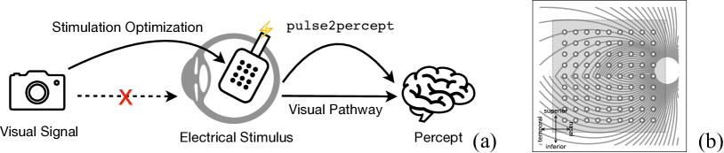
Figure 1: (a) A schematic overview of the stimulation optimization for retinal prostheses. (b) A retinal implant with a $9\times 9$ electrode grid on the axon map [5].

As one of the notable early papers of Invertible Neural Networks (INNs), Dinh et al. [9] propose to use INNs for density estimation tasks. Throughout a series of non-volume transformation processes, the normalizing flow [24] (total probability mass) is preserved, which ensures that the resulting distribution remains a valid probability distribution. Conceptually, INNs are naturally suitable to construct an autoencoder [16], as the forward and backward direction of the INN should always form a perfect encoder-decoder pair. Nguyen et al. [22] train an INN autoencoder with an artificial bottleneck, created by setting several elements to zero before the inverse pass. Sorrenson et al. [27] train autoencoders with likelihood on novel flow architectures that do not rely on coupling and are not dimension preserving. Furthermore, Ardizzone et al. first propose an INN variant to solve inverse problems [3] and an extension to INNs with explicit controls, namely Conditional Invertible Neural Networks (cINNs) [2].

In this work, we follow an INN [3] and a cINN approach [2] to learn a computational model for the visual pathway (Fig. 1a) and automatically obtain the inverse mapping from percept to stimulus thanks to the intrinsic feature of invertibility. Furthermore, INNs are generative and can be leveraged to become bijective to solve inverse problems [3]. In addition, by imposing conditioning to the INN, the generated inverse input (optimized stimulus, see Fig. 2) shall follow the desired constraint. We compare the reconstruction quality of the predicted percepts using cINNs to other approaches, including trivial downsampling, a linear model, feed-forward and invertible neural networks, and address the promising optimization for retinal prosthetic stimuli.

2 Methods

2.1 Stimulation Optimization

We begin by formulating the in silico optimization problem for retinal prosthetic stimuli. Let ${f}$ represent the function of the visual pathway (Fig. 1), which uses the electrical stimulus $\mathbf{x}_{s}$ from the implanted electrode array as input and produces the percept $\mathbf{y}_{p}$ as output. We assume that $f_{\phi}$ can simulate ${f}$, where $\phi$ denotes the parameters of the computational model, such as the Axon Map Model [5]. The desired encoding function $g_{\theta}:\tilde{\mathbf{x}}\mapsto\mathbf{x}_{s}$ from the visual signal (target) $\tilde{\mathbf{x}}$ to the stimulus ${\mathbf{x}_{s}}$ can be found with the following optimization problem:

$$\min_{\theta}\mathcal{L}_{\mathrm{MSE}}\left(\tilde{\mathbf{x}},f_{\phi}\left(g_{\theta}\left(\tilde{\mathbf{x}}\right)\right)\right),$$ (1)

where the Mean Squared Error (MSE) serves as the objective function $\mathcal{L}_{\mathrm{MSE}}$. We employ a neural network to construct $g_{\theta}$ with learnable parameters $\theta$.

2.2 Invertible Neural Network

Given a random variable $\mathbf{z}=h(\mathbf{x})$ with a known and tractable density, e.g., a spherical multivariate normal distribution $\mathbf{z}\sim\pi(\mathbf{z})=\mathcal{N}(\mathbf{z};\mathbf{0},\mathbf{I}))$, a data point $\mathbf{x}$ from an i.i.d. dataset $\mathcal{D}$ can be generated by $\mathbf{x}=h^{-1}(\mathbf{z})$ for an invertible function $h$. In this work, we use Invertible Neural Networks (INNs) to express $h$. Following the change of variables theorem, the probability density function of such a model, given a data point $\mathbf{x}$, can be written as:

$$p(\mathbf{x})=\pi(\mathbf{z}=h(\mathbf{x}))\left|\det\frac{\partial h(\mathbf{x})}{\partial\mathbf{x}^{T}}\right|,$$ (2)

where $\mathbf{J}_{h}(\mathbf{x})=\partial h(\mathbf{x})/\partial\mathbf{x}^{T}$ is the Jacobian matrix of $h$ at $\mathbf{x}$.

If a process $s:\mathbf{x}_{D}\in\mathbb{R}^{D}\mapsto\mathbf{y}_{d}\in\mathbb{R}^{d}$ is not bijective with $D>d$, we can introduce a latent random variable $\mathbf{z}_{K}\sim\pi(\mathbf{z}_{K})=\mathcal{N}(\mathbf{z}_{K};\mathbf{0},\mathbf{I}_{K}))$ with $K=D-d$, as proposed by Ardizzone et al. [3]. We then construct an invertible process $h:\mathbf{x}_{D}\mapsto[\mathbf{y}_{d},\mathbf{z}_{K}]$ with $h(\mathbf{x}_{D})=[h_{\mathbf{y}_{d}}(\mathbf{x}_{D}),h_{\mathbf{z}_{K}}(\mathbf{x}_{D})]$ and $h_{\mathbf{y}_{d}}(\mathbf{x}_{D})\approx s(\mathbf{x}_{D})$. Similar to [3], we apply a supervised Mean Squared Error (MSE) loss on $\mathbf{y}_{d}$ with $\mathcal{L}_{\mathrm{MSE}}=\mathbb{E}[(\mathbf{y}_{d}-h_{\mathbf{y}_{d}}(\mathbf{x}_{D}))^{2}]$ and an unsupervised Maximum Mean Discrepancy (MMD) loss [13] in terms of $\mathbf{x}_{D}$ and $\mathbf{z}_{K}$, respectively. The MMD loss enforces two distributions $P_{M}$ and $P_{M^{\prime}}$ to be identical and is formulated as:

$$\mathcal{L}_{\mathrm{MMD}}(p_{M},p_{M^{\prime}})=\left(\mathbb{E}_{i,j}[k(\mu_{i},\mu_{j})-2k(\mu_{i},\mu_{j}^{\prime})+k(\mu_{i}^{\prime},\mu_{j}^{\prime})]\right)^{\frac{1}{2}},$$ (3)

where $\mathbb{E}$ denotes the expected value and $\{\mu\},\{\mu^{\prime}\}$ are two sets of samples according to the distributions $\mu\sim p_{M}$ and $\mu^{\prime}\sim p_{M^{\prime}}$, respectively.

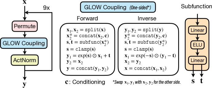
Figure 8: We follow [2] to design the INN and cINN architectures with GLOW coupling layers [15]. The conditional input $\mathbf{c}$ in both forward and inverse GLOW coupling blocks is the only difference between the INN and the cINN approach. The affine coupling layer [9, 15] is implemented with GLOWCouplingBlock in [1].

As suggested in [3, 30], we utilize the inverse multiquadratic kernel $k(\mu,\mu^{\prime})=\left(1+\left\|(\mu-\mu^{\prime})/\sigma\right\|_{2}^{2}\right)^{-1}$. The MMD loss on $\mathbf{x}_{D}$ forces it to match the prior with $\mathcal{L}_{\mathrm{MMD}}(p(\mathbf{x}_{D}),p(h^{-1}([\mathbf{y}_{d},\mathbf{z}_{K}])))$ and is optional. The MMD loss on $\mathbf{z}_{K}$ forces it to match the normal distribution with $\mathcal{L}_{\mathrm{MMD}}(p(h(\mathbf{x}_{D})),p(\mathbf{y}_{d})p(\mathbf{z}_{K}))$. Moreover, we follow [3] to pad $\mathbf{x}_{D}$ to match the dimensionality if necessary. Under the constraint of the invertible network architecture, both $h$ and $h^{-1}$ can be explicitly trained in both directions with a guaranteed invertible relation. Numerous invertible neural network architecture designs have been proposed to ensure that the inverse and the Jacobian determinant are easily computed, such as additive coupling layer [8], affine coupling layer [9], GLOW (including ActNorm and invertible $1\times 1$ convolution) [15]. The implementation details of the architecture in this work are presented in Section 3.3 and visualized in Fig. 8 in Appendix H.

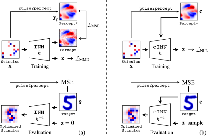
Figure 2: Training and evaluation pipelines for the stimulation optimization with (a) invertible neural networks and (b) conditional invertible neural networks.

2.3 Conditional Invertible Neural Network

We first discuss the maximum likelihood training for non-conditional INNs. With $\mathbf{x}$ and $\mathbf{z}$ sharing the identical dimensionality, the bijective normalizing flow $h$ can be trained by maximizing likelihood of $\mathbf{x}$, which is equivalent to minimizing the Negative Log-Likelihood (NLL) loss:

$$\mathcal{L}_{\mathrm{NLL}}=-\log(p(\mathbf{x})) =-\log(\mathcal{N}(h(\mathbf{x});\mathbf{0},\mathbf{I})))-\log\left|\det\mathbf{J}_{h}(\mathbf{x})\right|$$

$$\simeq\frac{1}{2}\|h(\mathbf{x})\|_{2}^{2}-\log\left|\det\mathbf{J}_{h}(\mathbf{x})\right|.$$ (4)

Within the local coupling blocks [9], conditioning features $\mathbf{c}$ can be integrated into both directions of the network by concatenating to the subfunctions with $\mathbf{z}=h(\mathbf{x};\mathbf{c})$ and $\mathbf{x}=h^{-1}(\mathbf{z};\mathbf{c})$, forming Conditional Invertible Neural Networks (cINNs) [2]. Accordingly, the NLL loss for cINN maximum likelihood training is formulated as $\mathcal{L}_{\mathrm{NLL}}\simeq\frac{1}{2}\|h(\mathbf{x};\mathbf{c})\|_{2}^{2}-\log\left|\det\mathbf{J}_{h}(\mathbf{x})\right|$. As shown in Fig. 2b, we train the cINN by minimizing the NLL loss in an unsupervised manner and use the predicted percept during the training and the MNIST target during the evaluation as the conditioning. The same invertible neural network architecture is used as in the INN experiments.

3 Experiments and Results

3.1 Axon Map Model

We create a virtual square retinal implant with a $9\times 9$ electrode grid (Fig. 1) and utilize the physiologically validated Axon Map Model [5] implemented in pulse2percept [4]. The percept intensity at location $(x,y)$ is calculated by:

$$I(x,y)=\exp\left(-\frac{(x-x_{\text{stim}})^{2}+(y-y_{\text{stim}})^{2}}{2\rho^{2}}-\frac{(x-x_{\text{soma}})^{2}+(y-y_{\text{soma}})^{2}}{2\lambda^{2}}\right),$$ (5)

with exponential decays in terms of the distances to the stimulus at $(x_{\text{stim}},y_{\text{stim}})$ and to the elongated soma at $(x_{\text{soma}},y_{\text{soma}})$, controlled by the constants $\rho$ and $\lambda$, respectively [4, 5]. In this paper, we select realistic and challenging $\rho=400\,\mu m$ and $\lambda=1550\,\mu m$ for all experiments (cf. [5]).

3.2 Datasets

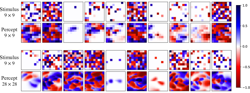
Figure 5: Examples of random samples from $9\times 9$ stimuli to both $9\times 9$ and $28\times 28$ percepts using Axon Map Model [5] implemented in pulse2percept [4].

In order to achieve generalizability, models are trained using 10,000,000 random stimulus-percept pairs and then evaluated with the MNIST test set [18]. The stimulus always has a resolution $9\times 9$ pixels (i.e., the number of the electrodes) and we experiment with both $9\times 9$ and $28\times 28$ pixels for percepts and the MNIST targets. Each stimulus-percept pair of the training set is generated by uniformly sampling in $[-1,+1]$ for each electrode and the prediction of pulse2percept with Axon Map Model. Additionally, for each stimulus, only a random percentage of electrodes are activated while the rest are set to zero. Examples of stimulus-percept pairs are showcased in Fig. 5 in Appendix F.

3.3 Implementation Details and Preliminary Remarks

We compare five different approaches to optimize retinal prosthetic stimuli. The visualization of the network architectures are depicted in Fig. 8 in Appendix H.

Downsampling. Trivial downsampling with a single learnable gain factor is applied to an input MNIST image as the visual signal.

Linear model. A single linear layer is used to learn the inverse transformation from percepts to stimuli. During the inference, the linear model outputs the optimized stimulus given an MNIST target image as the input.

Neural network. For the non-invertible neural network models, we use a residual architecture with blocks of convolutional layers, batch normalizations [14], and ELU activations [7].

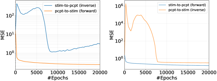
Figure 7: MSE loss values of the INN training [3] for percept-to-stimulus being the forward process (left) and for stimulus-to-percept being the forward process (right). We observe that the MSE loss values of inverse processes are always larger than the supervised forward processes, which implies that the invertibility using a supervised INN is not guaranteed. We report the results of the left setup in Table 1, as the optimized stimulus is desired.

Invertible neural network. We use the open-source library FrEIA [1] for the implementation of the invertible network. Each INN layer is formed by a random permutation layer, a GLOW coupling block [1, 15], and an ActNorm layer [15]. The subfunction inside the coupling block contains two ReLU-activated linear layers with a hidden dimension of 512. A stack of 9 INN layers is empirically found to be sufficient and no additional performance gains are observed beyond that. During the training, we try to define either stimulus-to-percept or percept-to-stimulus as the forward process. We compare the MSE loss of both sides and find that defining $h$ (Eq. 2) as the percept-to-stimulus mapping makes the inverse function $h^{-1}$ easier to train, as shown in Fig. 7 in Appendix G. We thus report the results based on this setup in Table 1.

Conditional invertible neural network. The cINN architecture follows the design of the INN, with the additional conditioning to the subfunction at each layer [2]. The percept or the MNIST target is concatenated as the conditioning during the training or the inference, respectively (Fig. 2b). The conditional input is first transformed with a learnable linear layer to a size of $9\times 9$ before being passed to the subfunction. As introduced in Section 2.3, the cINN is trained in an unsupervised manner only with the NLL loss (Eq. 2.3).

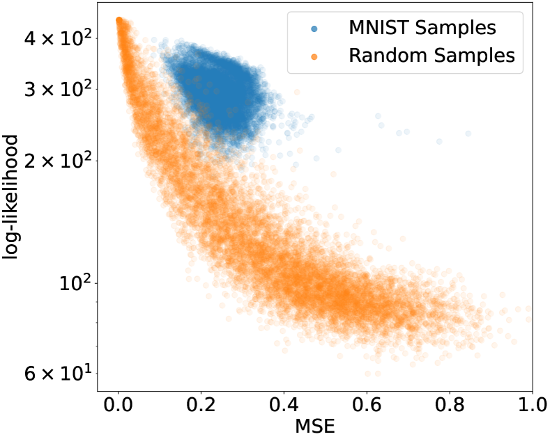
(a) Correlation between likelihood and MSE for MNIST and random samples.

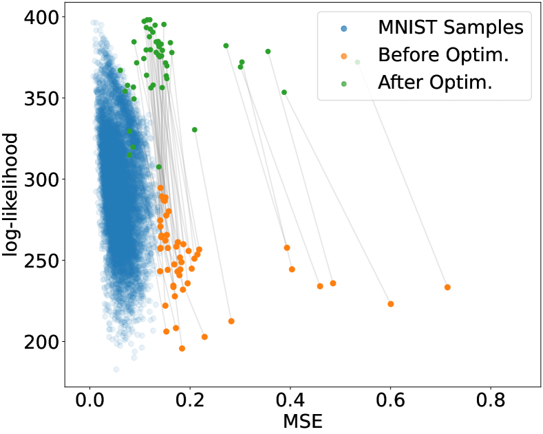
(b) Improved MSE with the optimized $\mathbf{z}$ for the 50 worst MNIST samples.

Figure 3: Investigation of log-likelihood and MSE loss in cINNs.

3.4 Likelihood and MSE

We illustrate whether the maximum likelihood training in the cINN approach leads to decrease the MSE loss [29]. The likelihood of the optimized stimulus depends on the likelihood of the latent $\mathbf{z}$ (Eq. 2.3). Fig. 3(a) shows the relationship between the log-likelihood of optimized stimulus (with $\mathbf{z}=\mathbf{0}$) and the MSE between the predicted percept and MNIST target (see Fig. 2b). For both random and MNIST samples, the correlation between the log-likelihood and the MSE can be observed. While setting $\mathbf{z}=\mathbf{0}$ should already give a good result, we further investigate if better $\mathbf{z}\neq\mathbf{0}$ can be found to yield higher likelihood and thus lower MSE. We select the worst 50 MNIST examples with the highest MSE and modify the latent $\mathbf{z}$ to maximize the total likelihood of optimized stimulus using gradient descent. Fig. 3(b) shows that the MSE is indeed decreased for most of the samples. Further optimization w.r.t. $\mathbf{z}$ can be addressed in future work.

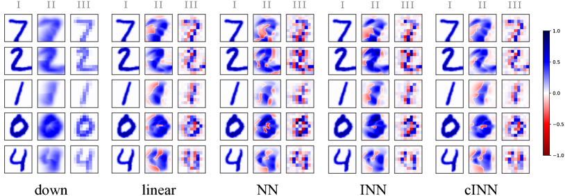
Figure 4: Visualization of the reconstruction quality with five approaches. (I) denotes the original MNIST targets. (II) denotes the predicted percepts of $28\times 28$ pixels based on (III) optimized stimuli of $9\times 9$ electrodes.

3.5 Reconstruction Quality

The visualization of the reconstruction quality with a percept resolution of $28\times 28$ pixels is illustrated in Fig. 4. We argue that negative stimulations (in red) can counteract the surrounding or elongated phosphenes, which is not applicable in downsampling. The predicted percepts (II) from the cINN show clearer turnings (e.g., the bottom left part in the image of 2) and cleaner corners of the visual field. The advantages can be confirmed by quantitative assessments. Four evaluation metrics are reported in Table 1, namely Mean Absolute Error (MAE), Structural Similarity Index Measure (SSIM) [32], Peak Signal-to-Noise Ratio (PSNR), and classification accuracy with a pre-trained classifier (ACC) [12, 34]. With an increased percept resolution, cINN outperforms other approaches in various metrics. The number of the parameters of each model is listed in Table 1. The supervised models (linear, non-invertible and invertible neural networks) are susceptible to a higher resolution due to the fully-connected layers in the architectures, while this dense layer is only used to concatenate the target or percept to the subfunctions in the cINN approach.

4 Discussion

4.1 Limitations

Our work relies on a pre-defined Axon Map Model with fixed $\rho$ and $\lambda$ for simulation. However, these parameters are largely patient- and implant-dependent [6] and not facile to determine in real-world scenarios (cf. [10, 11]). Additionally, we attempted to alter the dimensionality either on the input or output side and applied the MMD loss in INNs, which did not result in performance improvement. Finally, the pre-computed random samples, as illustrated in Fig. 3(a), are not sufficiently general, making the study of more complex datasets a challenge.

Table 1: Reconstruction quality evaluation from the predicted percepts to the original visual signals based on the optimized stimuli. Five approaches are compared with two resolutions (Res.) of the original MNIST input image of $9\times 9$ and $28\times 28$ pixels. Four evaluation metrics are reported, namely Mean Absolute Error (MAE), Structural Similarity Index Measure (SSIM), Peak Signal-to-Noise Ratio (PSNR), and classification accuracy with a pre-trained classifier (ACC). The number of the parameters of each model is listed. The top results are marked in red, while the second-best results are marked in blue.

Methods	Res.	MAE $\downarrow$	SSIM $\uparrow$	PSNR $\uparrow$	ACC $\uparrow$	#Param $\downarrow$
down		0.1682	0.7248	30.4149	0.4272	1
linear	9	0.1657	0.7246	30.6877	0.5608	6,561
NN	$\times$	0.1387	0.7799	31.9620	0.5572	946,512
INN	9	0.1785	0.7088	30.5656	0.4892	1,866,270
cINN		0.1373	0.7651	30.8940	0.5480	1,936,710
down		0.3432	0.3784	25.0973	0.2884	1
linear	28	0.3279	0.4770	25.1453	0.5884	63,504
NN	$\times$	0.3340	0.4901	25.2400	0.6192	4,270,900
INN	28	0.3231	0.4937	25.2729	0.5764	18,063,390
cINN		0.3136	0.4943	25.5161	0.5932	2,449,197

4.2 Outlook

We expect our future studies to progress in two directions. First, supervised training of INN [3] can be further explored using different invertible architecture designs and training strategies. Second, simulation experiments can be conducted on more complex datasets using other computational models to optimize stimuli.

5 Conclusion

We propose a stimulation optimization approach using conditional invertible neural networks for epiretinal implants and compare the reconstruction quality among downsampling, linear model, non-invertible and invertible neural networks. The cINN-based results outperform others w.r.t. various measures, especially with a higher resolution of visual inputs and percepts. Our findings highlight the potential application with this generative, invertible, and conditional neural network to enhance the quality of retinal prostheses.

5.0.1 Acknowledgements

This work was funded by the Deutsche Forschungsgemeinschaft (DFG, German Research Foundation) – grant 424556709/GRK2610.

Optimizing Retinal Prosthetic Stimuli with Conditional Invertible Neural Networks – Supplementary Material –

Appendix F Visualization

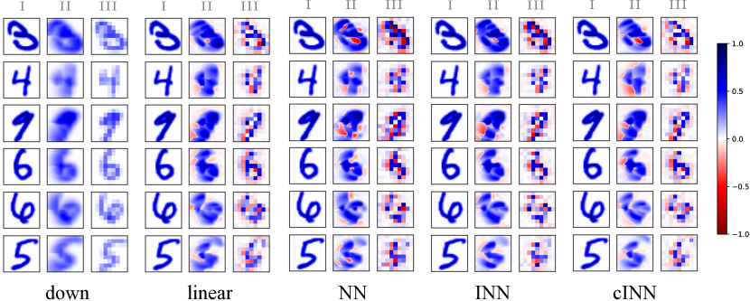
Figure 6: Visualization of the reconstruction quality with five approaches. (I) denotes the original MNIST targets. (II) denotes the predicted percepts of $28\times 28$ pixels based on (III) optimized stimuli of $9\times 9$ electrodes. Continued from Fig. 4.

Appendix G MSE Loss in INN Trainings

Appendix H Invertible Neural Network Architecture

References

- [1] Ardizzone, L., Bungert, T., Draxler, F., Köthe, U., Kruse, J., Schmier, R., Sorrenson, P.: Framework for Easily Invertible Architectures (FrEIA) (2018-2022), https://github.com/vislearn/FrEIA
- [2] Ardizzone, L., Kruse, J., Lüth, C., Bracher, N., Rother, C., Köthe, U.: Conditional invertible neural networks for diverse image-to-image translation. In: German Conference on Pattern Recognition. pp. 373–387 (2021)
- [3] Ardizzone, L., Kruse, J., Rother, C., Köthe, U.: Analyzing inverse problems with invertible neural networks. In: International Conference on Learning Representations (2018)
- [4] Beyeler, M., Boynton, G.M., Fine, I., Rokem, A.: pulse2percept: A python-based simulation framework for bionic vision. In: Proceedings of the 16th Python in Science Conference. pp. 81–88 (2017)
- [5] Beyeler, M., Nanduri, D., Weiland, J.D., Rokem, A., Boynton, G.M., Fine, I.: A model of ganglion axon pathways accounts for percepts elicited by retinal implants. Scientific Reports 9(1), 1–16 (2019)
- [6] Beyeler, M., Sanchez-Garcia, M.: Towards a smart bionic eye: Ai-powered artificial vision for the treatment of incurable blindness. Journal of Neural Engineering 19(6), 063001 (2022)
- [7] Clevert, D.A., Unterthiner, T., Hochreiter, S.: Fast and accurate deep network learning by exponential linear units (elus). In: International Conference on Learning Representations (2016)
- [8] Dinh, L., Krueger, D., Bengio, Y.: NICE: non-linear independent components estimation. In: International Conference on Learning Representations, Workshop Track Proceedings (2015)
- [9] Dinh, L., Sohl-Dickstein, J., Bengio, S.: Density estimation using real nvp. In: International Conference on Learning Representations (2016)
- [10] Fauvel, T., Chalk, M.: Human-in-the-loop optimization of visual prosthetic stimulation. Journal of Neural Engineering 19(3), 036038 (2022)
- [11] Granley, J., Fauvel, T., Chalk, M., Beyeler, M.: Human-in-the-loop optimization for deep stimulus encoding in visual prostheses. In: Advances in Neural Information Processing Systems 36. pp. 79376–79398 (2023)
- [12] Granley, J., Relic, L., Beyeler, M.: Hybrid neural autoencoders for stimulus encoding in visual and other sensory neuroprostheses. In: Advances in Neural Information Processing Systems 35. pp. 22671–22685 (2022)
- [13] Gretton, A., Borgwardt, K., Rasch, M., Schölkopf, B., Smola, A.: A kernel method for the two-sample-problem. In: Advances in Neural Information Processing Systems 19. pp. 513–520 (2006)
- [14] Ioffe, S., Szegedy, C.: Batch normalization: Accelerating deep network training by reducing internal covariate shift. In: International Conference on Machine Learning. pp. 448–456. PMLR (2015)
- [15] Kingma, D.P., Dhariwal, P.: Glow: Generative flow with invertible 1x1 convolutions. In: Advances in Neural Information Processing Systems 31. pp. 10236–10245 (2018)
- [16] Kingma, D.P., Welling, M.: Auto-encoding variational bayes. In: International Conference on Learning Representations (2014)
- [17] Küçükoğlu, B., Rueckauer, B., Ahmad, N., van Steveninck, J.d.R., Güçlü, U., van Gerven, M.: Optimization of neuroprosthetic vision via end-to-end deep reinforcement learning. International Journal of Neural Systems 32(11), 2250052 (2022)
- [18] LeCun, Y., Bottou, L., Bengio, Y., Haffner, P.: Gradient-based learning applied to document recognition. Proceedings of the IEEE 86(11), 2278–2324 (1998)
- [19] Lohmann, T.K., Haiss, F., Schaffrath, K., Schnitzler, A.C., Waschkowski, F., Barz, C., van Der Meer, A.M., Werner, C., Johnen, S., Laube, T., et al.: The very large electrode array for retinal stimulation (vlars)—a concept study. Journal of Neural Engineering 16(6), 066031 (2019)
- [20] Luo, Y.H.L., Da Cruz, L.: The argus® ii retinal prosthesis system. Progress in Retinal and Eye Research 50, 89–107 (2016)
- [21] Mokwa, W., Goertz, M., Koch, C., Krisch, I., Trieu, H.K., Walter, P.: Intraocular epiretinal prosthesis to restore vision in blind humans. In: International Conference of the IEEE Engineering in Medicine & Biology Society (EMBC). pp. 5790–5793. IEEE (2008)
- [22] Nguyen, T.G.L., Ardizzone, L., Köthe, U.: Training invertible neural networks as autoencoders. In: German Conference on Pattern Recognition. pp. 442–455 (2019)
- [23] Relic, L., Zhang, B., Tuan, Y.L., Beyeler, M.: Deep learning–based perceptual stimulus encoder for bionic vision. In: Proceedings of the Augmented Humans International Conference 2022. pp. 323–325 (2022)
- [24] Rezende, D., Mohamed, S.: Variational inference with normalizing flows. In: International Conference on Machine Learning. pp. 1530–1538. PMLR (2015)
- [25] Roessler, G., Laube, T., Brockmann, C., Kirschkamp, T., Mazinani, B., Goertz, M., Koch, C., Krisch, I., Sellhaus, B., Trieu, H.K., et al.: Implantation and explantation of a wireless epiretinal retina implant device: observations during the epiret3 prospective clinical trial. Investigative Ophthalmology & Visual Science 50(6), 3003–3008 (2009)
- [26] Romeni, S., Zoccolan, D., Micera, S.: A machine learning framework to optimize optic nerve electrical stimulation for vision restoration. Patterns 2(7) (2021)
- [27] Sorrenson, P., Draxler, F., Rousselot, A., Hummerich, S., Zimmermann, L., Köthe, U.: Lifting architectural constraints of injective flows. In: International Conference on Learning Representations (2024)
- [28] van Steveninck, J.d.R., Güçlü, U., van Wezel, R., van Gerven, M.: End-to-end optimization of prosthetic vision. Journal of Vision 22(2.20), 1–14 (2022)
- [29] Theis, L., Oord, A.v.d., Bethge, M.: A note on the evaluation of generative models. In: International Conference on Learning Representations (2016)
- [30] Tolstikhin, I., Bousquet, O., Gelly, S., Schoelkopf, B.: Wasserstein auto-encoders. In: International Conference on Learning Representations (2018)
- [31] Walter, P., Mokwa, W.: Epiretinal visual prostheses. Der Ophthalmologe 102, 933–940 (2005)
- [32] Wang, Z., Bovik, A.C., Sheikh, H.R., Simoncelli, E.P.: Image quality assessment: from error visibility to structural similarity. IEEE Transactions on Image Processing 13(4), 600–612 (2004)
- [33] Waschkowski, F., Hesse, S., Rieck, A.C., Lohmann, T., Brockmann, C., Laube, T., Bornfeld, N., Thumann, G., Walter, P., Mokwa, W., et al.: Development of very large electrode arrays for epiretinal stimulation (vlars). BioMedical Engineering Online 13(1), 1–15 (2014)
- [34] Wu, Y., Karetic, I., Stegmaier, J., Walter, P., Merhof, D.: A deep learning-based in silico framework for optimization on retinal prosthetic stimulation. In: International Conference of the IEEE Engineering in Medicine & Biology Society (EMBC). pp. 1–4. IEEE (2023)
- [35] Wu, Y., Koch, L., Walter, P., Merhof, D.: Convolutional neural network-based inverse encoder for optimization of retinal prosthetic stimulation. Biomedical Engineering / Biomedizinische Technik 68(s1), 235 (2023)