Controller Adaptation via Learning Solutions of
Contextual Bayesian Optimization

Abstract

In this letter, we propose a framework for adapting the controller’s parameters based on learning optimal solutions from contextual black-box optimization problems. We consider a class of control design problems for dynamical systems operating in different environments or conditions represented by contextual parameters. The overarching goal is to identify the controller parameters that maximize the controlled system’s performance, given different realizations of the contextual parameters. We formulate a contextual Bayesian optimization problem in which the solution is actively learned using Gaussian processes to approximate the controller adaptation strategy. We demonstrate the efficacy of the proposed framework with a simulation-to-real example. We learn the optimal weighting strategy of a model predictive control for connected and automated vehicles interacting with human-driven vehicles from simulations and then deploy it in a real-time experiment.

Controller adaptation, contextual Bayesian optimization.

1 Introduction

Controller tuning generally aims to find controller parameters that optimize specific performance metrics. In recent years, controller tuning has received increasing attention in different control applications. Some popular approaches that have been presented in the literature include reinforcement learning [1, 2], Bayesian optimization (BO) [3, 4, 5], self-learning control [6], and Kalman filtering [7, 8]. While classical controller tuning approaches often focus on optimizing the controller for invariant systems, in practice, the system must operate under changing conditions, environments, or tasks such as throttle valve systems with different goal positions [9], advanced powertrain systems operating under different driving styles [10], or connected and automated vehicles interacting with diverse styles of human-driven vehicles [11, 12] and diverse traffic conditions resulting in activating safety constraints [13]. A potential approach to address this problem is contextual BO [14] which is an extension of BO that considers additional variables beyond the optimization variables. Berkenkamp et al.[15] presented a safe contextual BO framework in which the safe control parameters for the unobserved contexts can be found given the surrogate model transferred from observed contexts. Frohlich et al.[16] considered a learned dynamic model as contexts in contextual BO to transfer knowledge across different environmental conditions in autonomous racing. Xu et al.[17] proposed primal-dual contextual BO to handle time-varying disturbances for thermal control systems of smart buildings.

In this letter, we propose a framework that approximates a controller adaptation strategy for dynamical systems by leveraging the optimal solutions of contextual BO. We formulate the controller adaptation problem as a contextual BO problem in which the varying system and controller parameters are treated as contexts and optimization variables, respectively. We employ Gaussian processes (GPs) to learn the latent mapping from the contexts to the solutions of the BO problem and utilize an adaptive sampling technique for the contexts. Therefore, our proposed framework fits well in applications where the contexts can be sampled, such as simulation-to-real applications or optimal experiment design problems. The strategy learned from data obtained in observed situations can be utilized in unobserved situations to facilitate real-time adaptation of the control parameters.

We demonstrate the effectiveness of the framework in a simulation-to-real example related to model predictive control (MPC) for connected and automated vehicles (CAVs) interacting with human-driven vehicles (HDVs). The weights of the MPC objective function must be adapted appropriately with respect to human driving behavior. In real-time deployment, the controller must quickly adapt to diverse and time-varying human driving behavior, which can become infeasible. In our framework, we provide a weight adaptation strategy for the MPC given different HDV driving behaviors from simulations so that the desired performance can be achieved. We perform real-time experiments, in which the learned strategy is then utilized alongside the real human driving behavior obtained from inverse reinforcement learning to adapt the MPC.

The remainder of the letter is organized as follows. In Section 2, we provide the problem statement for controller adaptation. We present the framework for learning the controller adaptation strategy in Section 3 and provide an analysis on optimality bounds in Section 4. We demonstrate the framework and show the results in Section 5. Finally, we draw some conclusions in Section 6.

2 Controller Adaptation Problem

We consider the problem of designing a controller for a dynamic system with contextual parameters, which can vary depending on the tasks or change over time due to environmental conditions. For instance, these contextual parameters could represent the setpoints at which the system operates, the weights in a cost function describing system behavior, or the time-varying coefficients of the system dynamics. Let $\boldsymbol{\theta}\in\boldsymbol{\Theta}$ be a vector representing the system contextual parameters with a set of values $\boldsymbol{\Theta}$. We consider the system controlled by a controller with parameters that can be tuned or adapted to optimize performance. For example, the controller parameters might encompass the gains of a PID controller, the coefficients of a state-feedback control law, or the weights within an MPC cost function. Let ${\boldsymbol{z}\in\mathcal{Z}}$ be the vector of controller parameters. In the controller tuning problem, if the system contextual parameters $\boldsymbol{\theta}$ are fixed, we seek for the optimal controller parameters $\boldsymbol{z}^{*}$ so that a certain performance metric is optimized, i.e.,

$$\underset{\boldsymbol{z}\in\mathcal{Z}}{\operatorname*{maximize}}\textbf{}\;J(\boldsymbol{z},\boldsymbol{\theta}),$$ (1)

where $J:\mathcal{Z}\times\Theta\rightarrow\mathbb{R}$ is a performance metric function. We are interested in the problem of finding an adaptation strategy $\boldsymbol{\gamma}$ for control parameters $\boldsymbol{z}$ given different realizations of $\boldsymbol{\theta}$ in (1). The objective of the proposed framework is to learn the latent function $\boldsymbol{\gamma}:\Theta\rightarrow\mathcal{Z}$ in (1), i.e.,

$$\boldsymbol{z}^{*}=\boldsymbol{\gamma}(\boldsymbol{\theta}).$$ (2)

This solution can be valuable in real-time control applications, where using controller tuning is rather infeasible, as it can be used to adapt $\boldsymbol{z}$ given the values of $\boldsymbol{\theta}$ in case some system parameters have changed. In our approach, we consider that the performance metric $J$ has the following properties:

• $J$ is a black box of $\boldsymbol{z}$ and $\boldsymbol{\theta}$, i.e., we do not have an analytical expression for $J$ in terms of $\boldsymbol{z}$ and $\boldsymbol{\theta}$.

• We can only observe the output of $J$ by evaluating the state and input trajectories of the system through simulations or experiments; however, we do not have access to the first- or second-order derivatives.

• Observations of $J$ can be noisy with independent and identically distributed (i.i.d.) Gaussian noise.

• Obtaining the observations of $J$ may be expensive and/or complex. For example, it may involve conducting experiments or require mass simulations with different initial conditions to obtain the average performance metric.

Given the above properties of the performance metric and if the system contextual parameters $\boldsymbol{\theta}$ are fixed, BO [18] is a commonly used method to tune the controller parameters. In contrast, for systems with varying parameters, one can utilize contextual BO [14], an extension of BO that considers additional variables known as contexts. Therefore, in the next section, we recast (1) as a contextual black-box optimization problem in which $\boldsymbol{z}$ and $\boldsymbol{\theta}$ are considered as the optimization variable and the context, respectively, and propose to approximate the solutions of contextual BO using GPs.

3 Learning Solutions of Contextual Black-box Optimization

In this section, we first provide background information on GPs and contextual BO, followed by a discussion on the method to approximate the solutions of contextual BO.

3.1 Gaussian Process

A GP defines a distribution over functions where any finite subset of function values follows a multivariate Gaussian distribution [19]. A GP model of a scalar function $f(\boldsymbol{x})$, denoted as $\mathcal{G}\mathcal{P}_{f}(\boldsymbol{x})$, is specified by a mean function $m(\boldsymbol{x})$ and a covariance function (kernel) $\kappa(\boldsymbol{x},\boldsymbol{x}^{\prime})$ which are parameterized by some hyperparameters. Given a training dataset $\mathcal{D}=(\boldsymbol{X},\boldsymbol{Y})$, where $\boldsymbol{X}=[\boldsymbol{x}_{1}^{\top},\dots,\boldsymbol{x}_{N}^{\top}]^{\top}$ and $\boldsymbol{Y}=[y_{1},\dots,y_{N}]^{\top}$ are concatenated vectors of $N\in\mathbb{N}$ observed inputs and corresponding outputs, those hyperparameters can be learned by maximizing the likelihood [19]. Without loss of generality, we consider a zero mean function in our exposition. At a new input $\boldsymbol{x}_{*}$, the GP prediction is a Gaussian distribution $\mathcal{N}(\mu_{*},\sigma_{*})$ that is computed by

$$\mu_{*} =\mu(\boldsymbol{x}_{*})=\mathbf{K}_{*}(\mathbf{K}+\sigma_{n}^{2}\mathbb{I})^{-1}\mathbf{Y},$$ (3a)

$$\sigma_{*}^{2} =\sigma^{2}(\boldsymbol{x}_{*})=\mathbf{K}_{\star\star}-\mathbf{K}_{*}(\mathbf{K}+\sigma_{n}^{2}\mathbb{I})^{-1}\mathbf{K}_{*}^{T},$$ (3b)

where $K_{*}=[\kappa(\boldsymbol{x}_{*},\boldsymbol{x}_{1}),\dots,\kappa(\boldsymbol{x}_{*},\boldsymbol{x}_{N})]$, $K_{\star\star}=\kappa(\boldsymbol{x}_{*},\boldsymbol{x}_{*})$, $K$ is the covariance matrix with elements $K_{ij}=\kappa(\boldsymbol{x}_{i},\boldsymbol{x}_{j})$, $\sigma_{n}^{2}$ is the noise variance, and $\mathbb{I}$ is the $N\times N$ identity matrix.

3.2 Contextual Bayesian Optimization

Contextual BO [14] is an extension of BO that aims to solve a class of black-box optimization problems with contexts that are not part of the optimization variables. Recall that in the controller adaptation problem, we aim at maximizing a black-box function $J(\boldsymbol{z},\,\boldsymbol{\theta})$ in (1). We define $\mathcal{G}\mathcal{P}_{o}(\boldsymbol{z},\boldsymbol{\theta})$ as the surrogate model that learns $J(\boldsymbol{z},\,\boldsymbol{\theta})$. The kernel of the surrogate model can be formed by considering a product kernel of the kernels over context and variable spaces as follows [14]

$$\kappa\big{(}(\boldsymbol{z},\boldsymbol{\theta}),(\boldsymbol{z}^{\prime},\boldsymbol{\theta}^{\prime})\big{)}=\kappa_{z}(\boldsymbol{z},\boldsymbol{z}^{\prime}).\kappa_{\theta}(\boldsymbol{\theta},\boldsymbol{\theta}^{\prime}),$$ (4)

which implies two context-variable pairs are similar if the contexts are similar and the variables are similar. Given a realization of the context $\boldsymbol{\theta}$, the contextual BO is identical to the original BO and the algorithm works as follows. First, it optimizes an acquisition function $\xi$ to find the next candidate of the solution,

$$\boldsymbol{z}^{(j)}=\underset{\boldsymbol{z}\in\mathcal{Z}}{\operatorname*{arg\,max}}\;\xi\big{(}\mu_{o}(\boldsymbol{z},\boldsymbol{\theta}),\sigma_{o}(\boldsymbol{z},\boldsymbol{\theta})\big{)},$$ (5)

where $\mu_{o}$ and $\sigma_{o}$ are the posterior mean and standard deviation of $\mathcal{G}\mathcal{P}_{o}$. For example, the upper confidence bound (UCB) acquisition function was used in contextual BO in [14] which is given by

$$\xi\big{(}\mu_{o}(\boldsymbol{z},\boldsymbol{\theta}),\sigma_{o}(\boldsymbol{z},\boldsymbol{\theta})\big{)}=\mu_{o}(\boldsymbol{z},\boldsymbol{\theta})+\beta^{1/2}\sigma_{o}(\boldsymbol{z},\boldsymbol{\theta}).$$ (6)

Next, the output of the performance metric at that sampling candidate is evaluated and added to the training dataset to retrain the surrogate model. This process is repeated until a maximum number of iterations is reached, and the best-evaluated candidate is returned. In this letter, we use GPs to learn the latent mapping from the context $\boldsymbol{\theta}$ to the solution $\boldsymbol{z}^{*}$ returned from contextual BO. To do that, we impose the following assumption.

Assumption 1

The latent mapping from $\boldsymbol{\theta}$ to $\boldsymbol{z}^{*}$ can be approximated by a GP with an appropriate kernel, i.e., $\boldsymbol{z}^{*}=\boldsymbol{\gamma}(\boldsymbol{\theta})\sim\mathcal{G}\mathcal{P}_{s}(\boldsymbol{\theta})$. We call $\mathcal{G}\mathcal{P}_{s}(\boldsymbol{\theta})$ as the solution model.

Although $\boldsymbol{z}$ is generally a vector, we approximate $\boldsymbol{z}^{*}$ by multiple single-output GPs for simplicity, in which each element of $\boldsymbol{z}^{*}$ is learned by a single-output GP. Let $n_{z}$ be the dimension of $\boldsymbol{z}$ and $\boldsymbol{z}^{*}=[z_{1}^{*},\dots,z_{n_{z}}^{*}]^{T}$, then ${z_{i}^{*}\sim\mathcal{G}\mathcal{P}_{s,i}(\boldsymbol{\theta})}$, ${\forall i=1,\dots,n_{z}}$.

3.3 Adaptive Sampling for the Solution Model

To efficiently and rapidly learn the solution model, we adopt the concept from Bayesian experimental design, aiming to find the set of most informative sampling points by maximizing the information gain. Since finding the maximizer of information gain is NP-hard, a commonly employed approach is to use a greedy adaptive sampling algorithm. For a single-output GP, at each iteration, the greedy algorithm selects the sampling location with the highest variance, and the GP model is recursively updated with the data obtained from the new sampling location [20]. Thus, the adaptive sampling optimization problem for the solution model at each iteration $k$ to find the next sampling location of $\boldsymbol{\theta}$ is formulated as follows

$$\boldsymbol{\theta}^{(k)}=\operatorname*{argmax}_{\boldsymbol{\theta}\in\Theta}\;\sum_{i=1}^{n_{z}}\sigma_{s,i}^{2}(\boldsymbol{\theta}).$$ (7)

The algorithm is presented in Algorithm 2 and is summarized as follows. At each iteration $j\in\mathbb{N}$, we first propose the next sampling location $\boldsymbol{\theta}^{(j)}$ by solving the adaptive sampling optimization problem given the current solution model $\mathcal{G}\mathcal{P}_{s}^{(j-1)}$. Then, we fix $\boldsymbol{\theta}^{(j)}$ and apply an inner-loop contextual BO (Algorithm 1) to find the next candidate of the solution $\boldsymbol{z}^{(j)}$. Once the solution is obtained, we update the training dataset and retrain $\mathcal{G}\mathcal{P}_{s}$. These steps are repeated until a maximum number $j_{\max}$ of iterations is reached.

Algorithm 1 Inner-loop Bayesian optimization

1:$k_{\mathrm{max}}\in\mathbb{N}\setminus\{0\}$

2:procedure BayesOpt($\boldsymbol{\theta}$, $\mathcal{G}\mathcal{P}_{o}$)

3:     $\mathcal{G}\mathcal{P}_{o}^{(0)}\leftarrow\mathcal{G}\mathcal{P}_{o}$

4:     for $k=1,\dots,k_{\mathrm{max}}$ do

5:         Find the next solution candidate $\boldsymbol{z}^{(k)}$ by optimizing acquisition function given $\mathcal{G}\mathcal{P}_{o}^{(k-1)}$.

6:         Obtain an observation of the performance metric $J^{(k)}=J\Big{(}\boldsymbol{z}^{(k)},\boldsymbol{\theta}\Big{)}$.

7:         Add $(\boldsymbol{z}^{(k)},\boldsymbol{\theta},J^{(k)})$ to $\mathcal{D}_{o}$ (see Remark 3.1) and re-train the surrogate GP model to obtain $\mathcal{G}\mathcal{P}_{o}^{(k)}$.      

8:     return $\boldsymbol{z}^{*}$, $\mathcal{G}\mathcal{P}_{o}^{(k_{\max})}$

Algorithm 2 Outer-loop adaptive sampling

1:$j_{\mathrm{max}}\in\mathbb{N}\setminus\{0\}$, $\mathcal{G}\mathcal{P}_{s}^{(0)}$, $\mathcal{G}\mathcal{P}_{o}^{(0)}$

2:for $j=1,\dots,j_{\max}$ do

3:     Find next sampling location $\boldsymbol{\theta}^{(j)}$ of the context by solving the adaptive sampling problem given $\mathcal{G}\mathcal{P}_{s}^{(j-1)}$.

4:     $\boldsymbol{z}^{(j)*},\mathcal{G}\mathcal{P}_{o}^{(j)}\leftarrow$ BayesOpt($\boldsymbol{\theta}^{(j)},\mathcal{G}\mathcal{P}_{o}^{(j-1)}$) (see Algorithm 1)

5:     Add $(\boldsymbol{\theta}^{(j)},\boldsymbol{z}^{(j)*})$ to $\mathcal{D}_{s}$ and re-train the solution GP model to obtain $\mathcal{G}\mathcal{P}_{s}^{(j)}$.

6:return $\mathcal{G}\mathcal{P}_{s}^{(j_{\max})}$

Remark 3.1.

In Algorithm 1, we reuse the GP surrogate model trained on data from previous contexts to enable knowledge transfer to a new context [15, 16], which makes the training data size of $\mathcal{G}\mathcal{P}_{o}$ larger over the iterations. Thus, if the training dataset exceeds the maximum size, a heuristic rule [21] can be used so that the old data is replaced by new data observation.

4 Analysis on Optimality Bound

Let $\epsilon_{n}=\left\lvert J(\boldsymbol{z}_{n}^{**},\boldsymbol{\theta}_{n})-J(\mu_{s}(\boldsymbol{\theta}_{n}),\boldsymbol{\theta}_{n})\right\rvert$ be the optimality error where $\boldsymbol{z}_{n}^{**}$ is the true maximizer of $J$ given the context $\boldsymbol{\theta}_{n}$. In this section, inspired by the prior work on contextual BO for bandit optimization [14], we derive a bound on $\epsilon_{n}$ that holds with probability at least $1-\delta$, where $\delta\in(0,1)$, under three technical assumptions presented in what follows.

Assumption 2

$J$ is a Lipschitz continuous function with a constant $L$.

Assumption 3

The sets $\mathcal{Z}$ and $\Theta$ are finite.

Assumption 4

The kernels for $\mathcal{G}\mathcal{P}_{o}$ and $\mathcal{G}\mathcal{P}_{s}$ are bounded over their domains, i.e., $\kappa_{o}(\cdot,\cdot)\leq\bar{\sigma}_{o}$ and $\kappa_{s,i}(\cdot,\cdot)\leq\bar{\sigma}_{s}$.

Assumption 3 can be practically satisfied if the domains for $\boldsymbol{z}$ and $\boldsymbol{\theta}$ are compact and a dense discretization is applied. Assumption 4 is commonly imposed to ensure bounded variances for the GP predictions [20]. In contrast, verifying Assumption 2 and determining a suitable Lipschitz constant might be challenging in practice, since $J$ can be a black-box function. Nonetheless, this assumption is necessary to quantify the optimality bound.

Lemma 4.2.

If $\beta\geq 2\log(2\left\lvert\mathcal{Z}\right\rvert\left\lvert\Theta\right\rvert/\delta)$, then

$$\left\lvert J(\boldsymbol{z}_{n}^{**},\boldsymbol{\theta}_{n})-J(\boldsymbol{z}^{*}_{n},\boldsymbol{\theta}_{n})\right\rvert\leq 2\sqrt{\beta\bar{\sigma}_{o}},$$ (8)

holds with probability greater than $1-\delta/2$.

Proof 4.3.

Using the Chernoff bound for Gaussian distribution and the union bound, we obtain

$$\left\lvert J(\boldsymbol{z},\boldsymbol{\theta})-\mu_{o}(\boldsymbol{z},\boldsymbol{\theta})\right\rvert\leq\sqrt{\beta}\sigma_{o}(\boldsymbol{z},\boldsymbol{\theta}),\,\forall\boldsymbol{z}\in\mathcal{Z},\boldsymbol{\theta}\in\Theta,$$ (9)

with probability greater than $1-\left\lvert\mathcal{Z}\right\rvert\left\lvert\Theta\right\rvert\exp(-\beta/2)$. Thus by choosing $\left\lvert\mathcal{Z}\right\rvert\left\lvert\Theta\right\rvert\exp(-\beta/2)\leq\delta/2$, we obtain

$$\beta\geq 2\log(2\left\lvert\mathcal{Z}\right\rvert\left\lvert\Theta\right\rvert/\delta),$$ (10)

so that (9) holds with probability greater than $1-\delta/2$.

Next, following Lemma 4.1 in [14], if (9) holds then

$$\begin{split}&\left\lvert J(\boldsymbol{z}_{n}^{**},\boldsymbol{\theta}_{n})-J(\boldsymbol{z}^{*}_{n},\boldsymbol{\theta}_{n})\right\rvert=J(\boldsymbol{z}_{n}^{**},\boldsymbol{\theta}_{n})-J(\boldsymbol{z}^{*}_{n},\boldsymbol{\theta}_{n})\\ &\quad\leq\sqrt{\beta}\sigma_{o}(\boldsymbol{z}^{*}_{n},\boldsymbol{\theta}_{n})+\mu_{o}(\boldsymbol{z}^{*}_{n},\boldsymbol{\theta}_{n})-J(\boldsymbol{z}^{*}_{n},\boldsymbol{\theta}_{n})\\ &\quad\leq 2\sqrt{\beta}\sigma_{o}(\boldsymbol{z}^{*}_{n},\boldsymbol{\theta}_{n}),\\ \end{split}$$ (11)

where the first inequality results from

$$\begin{split}J(\boldsymbol{z}_{n}^{**},\boldsymbol{\theta}_{n})&\leq\mu_{o}(\boldsymbol{z}^{**}_{n},\boldsymbol{\theta}_{n})+\sqrt{\beta}\sigma_{o}(\boldsymbol{z}^{**}_{n},\boldsymbol{\theta}_{n})\\ &\leq\mu_{o}(\boldsymbol{z}^{*}_{n},\boldsymbol{\theta}_{n})+\sqrt{\beta}\sigma_{o}(\boldsymbol{z}^{*}_{n},\boldsymbol{\theta}_{n}).\end{split}$$ (12)

From Assumption 4, we have

$$\sigma_{o}^{2}(\boldsymbol{z}^{*}_{n},\boldsymbol{\theta}_{n})\leq\kappa_{o}\Big{(}(\boldsymbol{z}^{*}_{n},\boldsymbol{\theta}_{n}),(\boldsymbol{z}^{*}_{n},\boldsymbol{\theta}_{n})\Big{)}\leq\bar{\sigma}_{o}.$$ (13)

Combining (11) and (13) leads to (8), the proof is thus complete.

Lemma 4.4.

Let ${c_{2}=\sqrt{2\log\big{(}2n_{z}|\Theta|/\delta\big{)}}}$. Then

$$\left\lvert J(\boldsymbol{z}^{*}_{n},\boldsymbol{\theta}_{n})-J(\mu_{s}(\boldsymbol{\theta}_{n}),\boldsymbol{\theta}_{n})\right\rvert\leq Lc_{2}n_{z}\sqrt{\bar{\sigma}_{s}},$$ (14)

holds with probability greater than $1-\delta/2$.

Proof 4.5.

From Assumption 2, since $J$ is a Lipschitz continuous function with a constant $L$, we have

$$\left\lvert J(\boldsymbol{z}^{*}_{n},\boldsymbol{\theta}_{n})-J(\mu_{s}(\boldsymbol{\theta}_{n}),\boldsymbol{\theta}_{n})\right\rvert\leq L\left\lVert\boldsymbol{z}^{*}_{n}-\mu_{s}(\boldsymbol{\theta}_{n})\right\rVert.$$ (15)

Next, we quantify the bound $\left\lVert\boldsymbol{z}^{*}_{n}-\mu_{s}(\boldsymbol{\theta}_{n})\right\rVert$. From the Cauchy–Schwarz inequality

$$\left\lVert\boldsymbol{z}^{*}_{n}-\mu_{s}(\boldsymbol{\theta}_{n})\right\rVert^{2}\leq n_{z}\sum_{i=1}^{n_{z}}\left\lvert\boldsymbol{z}^{*}_{n,i}-\mu_{s,i}(\boldsymbol{\theta}_{n})\right\rvert^{2}.$$ (16)

For single-output GP, from Chernoff bound and the union bound we have

$$|\boldsymbol{z}^{*}_{n,i}-\mu_{s,i}(\boldsymbol{\theta}_{n})|\leq c_{2}\sigma_{s,i}(\boldsymbol{\theta}_{n}),\,\forall\boldsymbol{\theta}_{n}\in\Theta,$$ (17)

with probability greater than $1-|\Theta|\exp(-c_{2}^{2}/2)$. Thus,

$$\sum_{i=1}^{n_{z}}\left\lvert\boldsymbol{z}^{*}_{n,i}-\mu_{s,i}(\boldsymbol{\theta}_{n})\right\rvert^{2}\leq c_{2}^{2}\sum_{i=1}^{n_{z}}\sigma_{s,i}^{2}(\boldsymbol{\theta}_{n}),\,\forall\boldsymbol{\theta}_{n}\in\Theta$$ (18)

holds with probability greater than $1-n_{z}|\Theta|\exp(-c_{2}^{2}/2)$. Therefore,

$$\left\lvert J(\boldsymbol{z}^{*}_{n},\boldsymbol{\theta}_{n})-J(\mu_{s}(\boldsymbol{\theta}_{n}),\boldsymbol{\theta}_{n})\right\rvert\leq Lc_{2}\sqrt{\sum_{i=1}^{n_{z}}\sigma_{s,i}^{2}(\boldsymbol{\theta}_{n})},\,$$ (19)

$\forall\boldsymbol{\theta}_{n}\in\Theta,$ holds with probability greater than $1-n_{z}|\Theta|\exp(-c_{2}^{2}/2)$. We set $n_{z}|\Theta|\exp(-c_{2}^{2}/2)=\delta/2$ which yields

$$c_{2}=\sqrt{2\log\big{(}2n_{z}|\Theta|/\delta\big{)}},$$ (20)

so that (19) holds with probability greater than $1-\delta/2$. From Assumption 4, we have

$$\sigma_{s,i}^{2}(\boldsymbol{\theta}_{n})\leq\kappa_{o,i}(\boldsymbol{\theta}_{n},\boldsymbol{\theta}_{n})\leq\bar{\sigma}_{s}.$$ (21)

Combining (19) and (21), we obtain (14).

Theorem 4.6.

If $\beta\geq 2\log(2\left\lvert\mathcal{Z}\right\rvert\left\lvert\Theta\right\rvert/\delta)$ then

$$\epsilon_{n}\leq 2\sqrt{\beta\bar{\sigma}_{o}}+Lc_{2}n_{z}\sqrt{\bar{\sigma}_{s}}$$ (22)

holds for all $\boldsymbol{\theta}_{n}\in\Theta$ with probability greater than $1-\delta$.

Proof 4.7.

From the triangle inequality, we have

$$\begin{multlined}\epsilon_{n}\leq\left\lvert J(\boldsymbol{z}^{**}_{n},\boldsymbol{\theta}_{n})-J(\boldsymbol{z}^{*}_{n},\boldsymbol{\theta}_{n})\right\rvert\\ +\left\lvert J(\boldsymbol{z}^{*}_{n},\boldsymbol{\theta}_{n})-J(\mu_{s}(\boldsymbol{\theta}_{n}),\boldsymbol{\theta}_{n})\right\rvert,\end{multlined}\epsilon_{n}\leq\left\lvert J(\boldsymbol{z}^{**}_{n},\boldsymbol{\theta}_{n})-J(\boldsymbol{z}^{*}_{n},\boldsymbol{\theta}_{n})\right\rvert\\ +\left\lvert J(\boldsymbol{z}^{*}_{n},\boldsymbol{\theta}_{n})-J(\mu_{s}(\boldsymbol{\theta}_{n}),\boldsymbol{\theta}_{n})\right\rvert,$$ (23)

where $\boldsymbol{z}^{*}_{n}$ is the solution from contextual BO given $\boldsymbol{\theta}_{n}$.

Lemmas 4.2 and 4.4 imply that

$$\left\lvert J(\boldsymbol{z}_{n}^{**},\boldsymbol{\theta}_{n})-J(\boldsymbol{z}^{*}_{n},\boldsymbol{\theta}_{n})\right\rvert>2\sqrt{\beta\bar{\sigma}_{o}},$$ (24)

holds with probability less than $\delta/2$, and

$$\left\lvert J(\boldsymbol{z}^{*}_{n},\boldsymbol{\theta}_{n})-J(\mu_{s}(\boldsymbol{\theta}_{n}),\boldsymbol{\theta}_{n})\right\rvert>Lc_{2}n_{z}\sqrt{\bar{\sigma}_{s}},$$ (25)

holds with probability less than $\delta/2$. Thus, using the union bound, we obtain

$$\begin{multlined}\left\lvert J(\boldsymbol{z}_{n}^{**},\boldsymbol{\theta}_{n})-J(\boldsymbol{z}^{*}_{n},\boldsymbol{\theta}_{n})\right\rvert>2\sqrt{\beta\bar{\sigma}_{o}}\\ \;\text{OR}\;\left\lvert J(\boldsymbol{z}^{*}_{n},\boldsymbol{\theta}_{n})-J(\mu_{s}(\boldsymbol{\theta}_{n}),\boldsymbol{\theta}_{n})\right\rvert>Lc_{2}n_{z}\sqrt{\bar{\sigma}_{s}},\end{multlined}\left\lvert J(\boldsymbol{z}_{n}^{**},\boldsymbol{\theta}_{n})-J(\boldsymbol{z}^{*}_{n},\boldsymbol{\theta}_{n})\right\rvert>2\sqrt{\beta\bar{\sigma}_{o}}\\ \;\text{OR}\;\left\lvert J(\boldsymbol{z}^{*}_{n},\boldsymbol{\theta}_{n})-J(\mu_{s}(\boldsymbol{\theta}_{n}),\boldsymbol{\theta}_{n})\right\rvert>Lc_{2}n_{z}\sqrt{\bar{\sigma}_{s}},$$ (26)

holds with probability less than $\delta$, which is equivalent to

$$\begin{multlined}\left\lvert J(\boldsymbol{z}_{n}^{**},\boldsymbol{\theta}_{n})-J(\boldsymbol{z}^{*}_{n},\boldsymbol{\theta}_{n})\right\rvert\leq 2\sqrt{\beta\bar{\sigma}_{o}}\\ \;\text{AND}\;\left\lvert J(\boldsymbol{z}^{*}_{n},\boldsymbol{\theta}_{n})-J(\mu_{s}(\boldsymbol{\theta}_{n}),\boldsymbol{\theta}_{n})\right\rvert\leq Lc_{2}n_{z}\sqrt{\bar{\sigma}_{s}},\end{multlined}\left\lvert J(\boldsymbol{z}_{n}^{**},\boldsymbol{\theta}_{n})-J(\boldsymbol{z}^{*}_{n},\boldsymbol{\theta}_{n})\right\rvert\leq 2\sqrt{\beta\bar{\sigma}_{o}}\\ \;\text{AND}\;\left\lvert J(\boldsymbol{z}^{*}_{n},\boldsymbol{\theta}_{n})-J(\mu_{s}(\boldsymbol{\theta}_{n}),\boldsymbol{\theta}_{n})\right\rvert\leq Lc_{2}n_{z}\sqrt{\bar{\sigma}_{s}},$$ (27)

holds with probability greater than $1-\delta$. Therefore, the inequality (22) holds with probability greater than $1-\delta$.

Remark 4.8.

Given (11) and (19), the optimality error depends on the upper bound of the predictive variances of both $\mathcal{G}\mathcal{P}_{o}$ and $\mathcal{G}\mathcal{P}_{s}$. That is the motivation for using the adaptive sampling approach and the UCB acquisition function so that the predictive uncertainty of GP models in the domain of interest is minimal.

5 Illustrative Example

In this section, we demonstrate the proposed framework with an example of learning the weight adaptation strategy of MPC for CAVs while interacting with an HDV. We consider an intersection scenario in a robotic testbed called the Information and Decision Science Lab’s Scaled Smart City (IDS3C) [22] shown in Fig. 1. We apply the proposed framework in a simulation-to-real manner, where the MPC weight adaptation strategy is learned from simulations and subsequently deployed to real-world experiments.

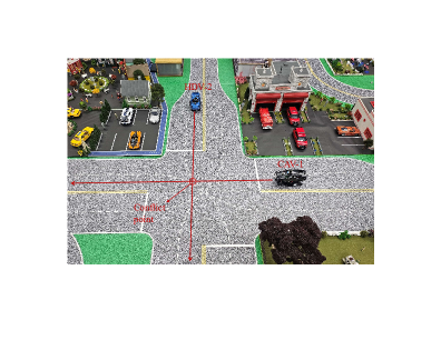
Figure 1: An intersection scenario with a CAV and an HDV.

5.1 Learning MPC Weight Adaptation Strategy for CAVs

Let CAV–$1$ and HDV–$2$ denote the vehicles involved in the intersection scenario. Next, we formulate an MPC problem for CAV–$1$ while interacting with HDV–$2$. The dynamics of each vehicle $i$ are given by the double-integrator dynamics

$$\begin{split}p_{i,k+1}&=p_{i,k}+\Delta Tv_{i,k}+\frac{1}{2}\Delta T^{2}a_{i,k},\\ v_{i,k+1}&=v_{i,k}+\Delta Ta_{i,k},\\ \end{split}$$ (28)

where $\Delta T\in\mathbb{R}^{+}$ is the sampling time, $p_{i,k}\in\mathbb{R}$ is the longitudinal position of the vehicle to the conflict point at time $k$, and $v_{i,k}\in\mathbb{R}$ and $a_{i,k}\in\mathbb{R}$ are the speed and acceleration of the vehicle $i$ at time step $k$, respectively. The vectors of states and control inputs of vehicle $i$ are defined by $\mathbf{x}_{i,k}=[p_{i,k},v_{i,k}]^{\top}$ and $u_{i,k}=a_{i,k}$, respectively. We consider the following state and control constraints

$$v_{\text{min}}\leq v_{1,k+1}\leq v_{\text{max}},\;u_{\text{min}}\leq a_{i,k}\leq u_{\text{max}},\;\forall k\in\mathcal{I}_{t},$$ (29)

where $u_{\text{min}}$, $u_{\text{max}}\in\mathbb{R}$ are the minimum deceleration and maximum acceleration, respectively, and $v_{\text{min}}$, $v_{\text{max}}\in\mathbb{R}$ are the minimum and maximum speed limits, respectively. Moreover, we impose the following safety constraint

$$r^{2}-(p_{1,k+1}^{2}+p_{2,k+1}^{2})\leq 0,\;\forall k\in\mathcal{I}_{t},$$ (30)

to guarantee that the predicted distances between CAV–$1$ and HDV–$2$ are greater than a safe distance, where $r\in\mathbb{R}^{+}$ is a safety threshold. The MPC objective is formed based on the idea of finding a Nash equilibrium of a potential game that models the interaction between the CAV and the HDV [11] as given by

$$\sum_{k\in\mathcal{I}_{t}}\Big{(}\sum_{i=1,2}l_{i}(\mathbf{x}_{i,k+1},u_{i,k})+l_{12}(\mathbf{x}_{1,k+1},\mathbf{x}_{2,k+1})\Big{)},$$ (31)

where $\mathcal{I}_{t}=\{t,\dots,t+H-1\}$ is the set of time steps in the control horizon of length $H\in\mathbb{N}\setminus\{0\}$ at time step $t$. The individual objective $l_{i}(\cdot),\,i=1,2$ in (31) includes minimizing the control input for smoother movement and energy saving and minimizing the deviation from the maximum speed to reduce the travel time, i.e.,

$$l_{i}(\mathbf{x}_{i,k+1},u_{i,k})=\begin{bmatrix}\omega_{i,1}\\ \omega_{i,2}\end{bmatrix}^{\top}\begin{bmatrix}a_{i,k}^{2}\\ (v_{i,k+1}-v_{\text{max}})^{2}\end{bmatrix},$$ (32)

for $i=1,2$, where $\omega_{i,1},\omega_{i,2}\in\mathbb{R}^{+}$ is the vector of positive weights and let denote $\boldsymbol{\omega}_{i}=[\omega_{i,1},\omega_{i,2}]^{\top}$. The shared objective function takes the form of a logarithmic penalty function of the distance between two vehicles as follows

$$l_{12}(\mathbf{x}_{1,k+1},\mathbf{x}_{2,k+1})=-\omega_{12}\log\big{(}p_{1,k+1}^{2}+p_{2,k+1}^{2}+\epsilon\big{)},$$ (33)

where $\omega_{12}\in\mathbb{R}^{+}$ is a positive weight and $\epsilon\in\mathbb{R}^{+}$ is a small positive number to guarantee that the argument of the logarithmic penalty function is always positive.

The MPC problem for CAV–$1$ in this example is thus formulated as follows

$$\begin{split}&\underset{\{u_{1,k},u_{2,k}\}_{k\in\mathcal{I}_{t}}}{\operatorname*{minimize}}\;\quad\eqref{eq:mpc-obj-func}\\ &\text{subject to:}\\ &\quad\text{\eqref{eq:integrator}},\text{\eqref{eq:bound}},\text{\eqref{eq:safe-dist}},\;\forall k\in\mathcal{I}_{t},\,i=1,2.\end{split}$$ (34)

In the objective function of the MPC problem (34), $\boldsymbol{\omega}_{2}$ and ${\omega}_{12}$ that best describes the human driving behavior can be learned online using inverse reinforcement learning [11]. Given the learned values of $\boldsymbol{\omega}_{2}$ and ${\omega}_{12}$, the CAV’s objective weights $\boldsymbol{\omega}_{1}$ can be adapted to achieve the desired performance. In this example, the context and variable of contextual BO are $\boldsymbol{\theta}:=\log\boldsymbol{\omega}_{2}$ and $\boldsymbol{z}:=\log\boldsymbol{\omega}_{1}$, respectively. The solution model learns the latent mapping from $\log\boldsymbol{\omega}_{2}$ to $\log\boldsymbol{\omega}_{1}^{*}$, i.e., $\log\boldsymbol{\omega}_{1}^{*}\sim\mathcal{G}\mathcal{P}_{s}(\log\boldsymbol{\omega}_{2})$. Note that we fix the shared objective weight $\omega_{12}$ as the solution of the MPC problem does not change if all the weights are scaled by a positive factor.

Given the vehicle trajectories obtained from simulation where we use MPC with a vector of the weights ${\boldsymbol{\omega}=[\boldsymbol{\omega}_{1}^{\top},\boldsymbol{\omega}_{2}^{\top},{\omega}_{12}]^{\top}}$, we define a time-energy efficiency with collision penalty metric which is formed as follows

$$\begin{multlined}\tilde{J}_{\boldsymbol{\omega}}(\mathbf{x}_{\text{MPC}},\mathbf{u}_{\text{MPC}})=\lambda^{\mathrm{time}}t_{1,f}+\lambda^{\mathrm{acce}}\!\!\int_{t_{0}}^{t_{1,f}}u_{1}^{2}(t)\;dt\\ +\lambda^{\mathrm{coll}}\mathrm{sigmoid}\big{(}g^{\mathrm{coll}}(\mathbf{x}_{\text{MPC}})\big{)},\end{multlined}\tilde{J}_{\boldsymbol{\omega}}(\mathbf{x}_{\text{MPC}},\mathbf{u}_{\text{MPC}})=\lambda^{\mathrm{time}}t_{1,f}+\lambda^{\mathrm{acce}}\!\!\int_{t_{0}}^{t_{1,f}}u_{1}^{2}(t)\;dt\\ +\lambda^{\mathrm{coll}}\mathrm{sigmoid}\big{(}g^{\mathrm{coll}}(\mathbf{x}_{\text{MPC}})\big{)},$$ (35)

where $\lambda^{\mathrm{time}}$, $\lambda^{\mathrm{acce}}$, and $\lambda^{\mathrm{coll}}\in\mathbb{R}^{+}$ are constants. In (35), $t_{1,f}$ is the time that CAV–$1$ exits the control zone, $\int_{t_{0}}^{t_{1,f}}u_{1}^{2}(t)\;dt$ is to minimize the acceleration of CAV–$1$ from $t_{0}=0$ to $t_{1,f}$ to get indirect energy benefits, while $\mathrm{sigmoid}\big{(}g^{\mathrm{coll}}(\mathbf{x}_{\text{MPC}})\big{)}$ is the sigmoid penalty function [12] to approximate the indicator function of the safety constraint $g^{\mathrm{coll}}(\mathbf{x}_{\text{MPC}})\leq 0$. The function $g^{\mathrm{coll}}(\mathbf{x}_{\text{MPC}})$ is defined as the maximum of the left-hand side in (30) for the entire trajectory. Note that $\lambda^{\mathrm{coll}}$ is sufficiently large compared to $\lambda^{\mathrm{time}}$ and $\lambda^{\mathrm{acce}}$ to prioritize safety. We consider the performance metric in contextual BO as the negative average of $\tilde{J}_{\boldsymbol{\omega}}(\mathbf{x}_{\text{MPC}},\mathbf{u}_{\text{MPC}})$ across multiple simulations with $n_{s}\in\mathbb{N}$ i.i.d. initial positions and speeds of the vehicles, i.e.,

$$J(\boldsymbol{z},\boldsymbol{\theta}):=-\frac{1}{n_{s}}\sum_{n=1}^{n_{s}}\tilde{J}_{\boldsymbol{\omega}}\Big{(}\mathbf{x}^{(n)}_{\text{MPC}},\mathbf{u}_{\text{MPC}}^{(n)}\Big{)}$$ (36)

where $\Big{(}\mathbf{x}^{(n)}_{\text{MPC}},\mathbf{u}_{\text{MPC}}^{(n)}\Big{)}$ denotes the state and input trajectories in the $n$-th simulation.

5.2 Results

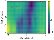
(a) Heat map for $\log_{10}(\omega_{1,1})$

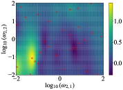
(b) Heat map for $\log_{10}(\omega_{1,2})$

Figure 2: Heat maps for the optimal weight adaptation strategy (in log scale). The red crosses represent the sampled values of $\log_{10}(\boldsymbol{\omega}_{2})$.

The learned weight adaptation strategy can be illustrated by heat maps in Fig 2 in which the sampled locations for the contexts are depicted by red crosses. We then validate the learned strategy for MPC weight adaptation through experiments. In our experimental setup, a robotic car is manually controlled by a human participant using a driving emulator to generate realistic human-driven vehicle behavior. Videos of the experiments can be found at https://sites.google.com/cornell.edu/lcss-exp. In Fig. 3, we show the position trajectories and speed profiles of the two vehicles in four specific simulations, each demonstrating different driving styles generated by the human participant. As can be seen from the figure, MPC with learned weight adaptation effectively tailors the behavior of connected and automated vehicles (CAVs) to accommodate varying human driving styles.

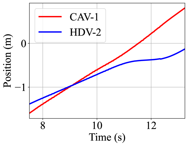
(a) Experiment $\#1$

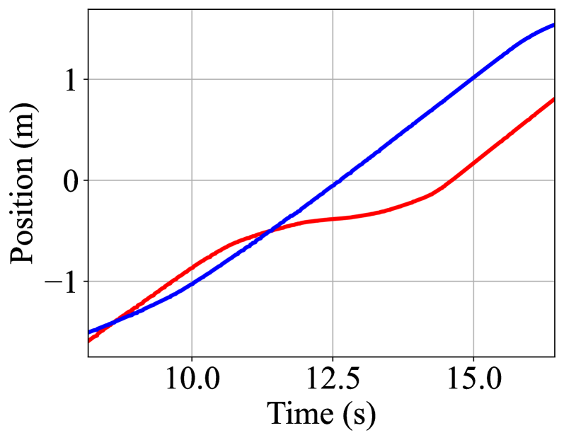
(b) Experiment $\#2$

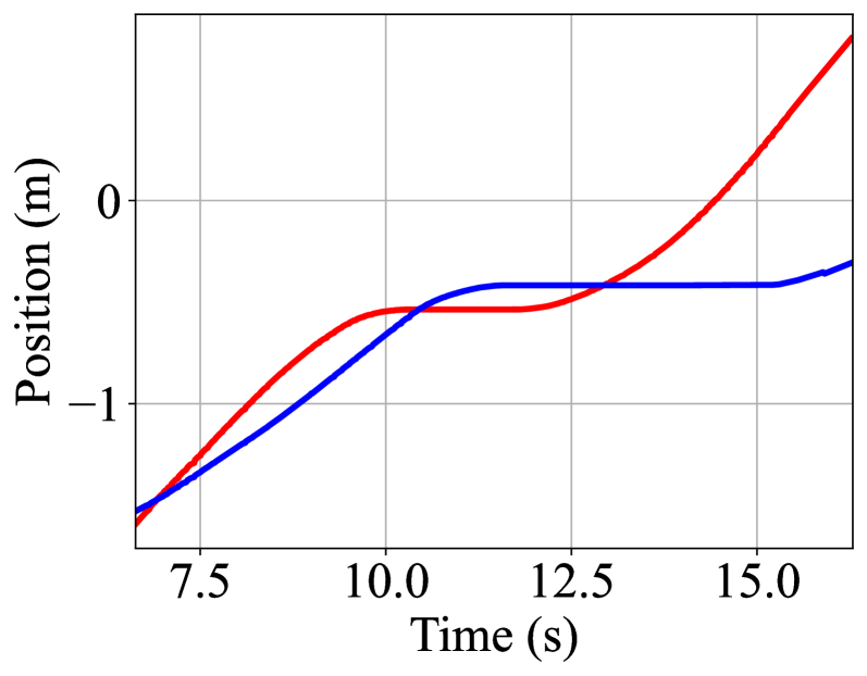
(c) Experiment $\#3$

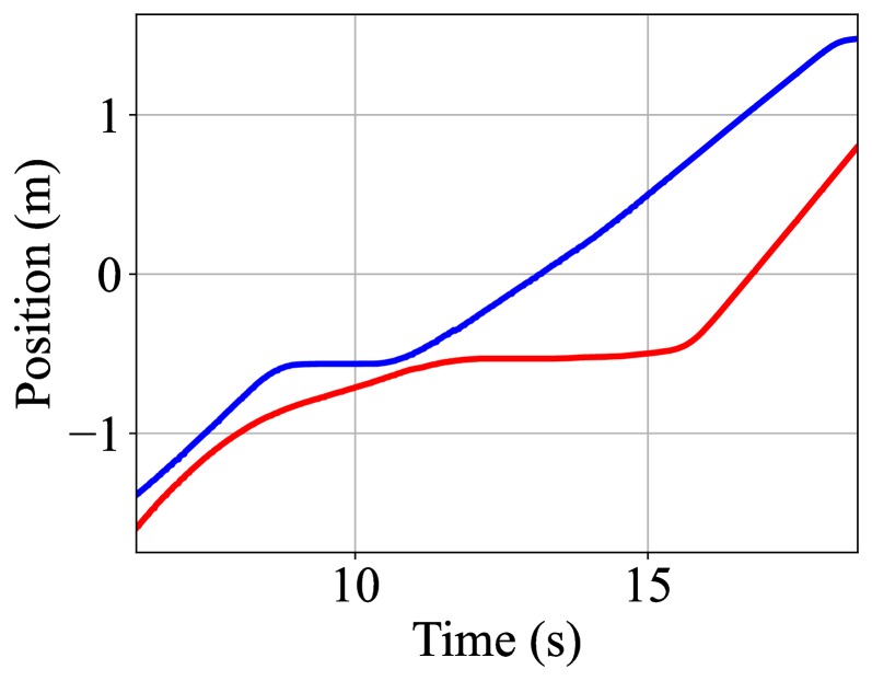
(d) Experiment $\#4$

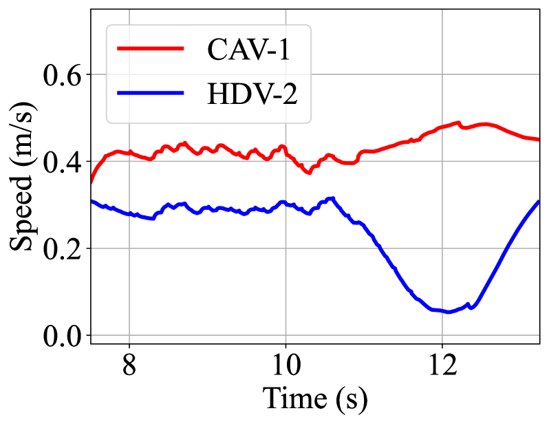
(e) Experiment $\#1$

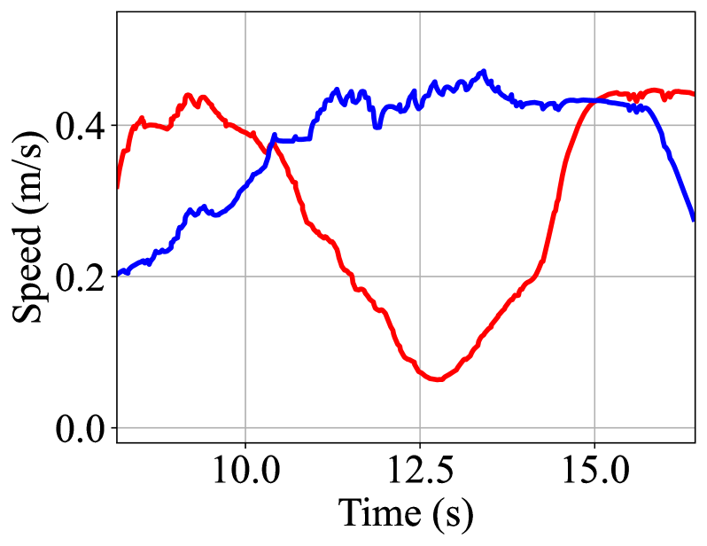
(f) Experiment $\#2$

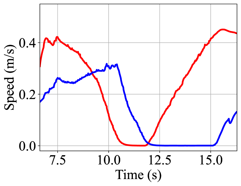
(g) Experiment $\#3$

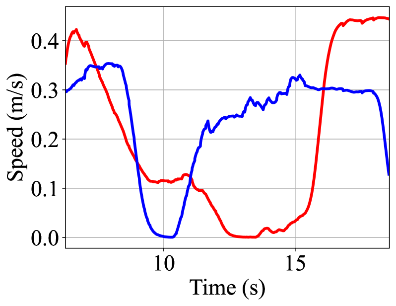
(h) Experiment $\#4$

Figure 3: Position trajectories (top figures) and speed profiles (bottom figures) of CAV–$1$ and HDV–$2$ in 4 experiments with different human driving styles.

6 Conclusions

In this letter, we proposed a framework to address the controller adaptation problem for dynamic systems with task-dependent or time-varying parameters via learning the solutions of contextual BO with GPs. We demonstrated the efficacy of the framework through a simulation-to-real application, where the weighting strategy of MPC for CAVs interacting with HDVs is learned from simulations and applied in real-time experiments. Future work should extend the framework to incorporate black-box constraints and relax the assumptions imposed for deriving the optimality bound in Section 4.

References

• [1] M. Mehndiratta, E. Camci, and E. Kayacan, “Automated tuning of nonlinear model predictive controller by reinforcement learning,” in 2018 IEEE/RSJ International Conference on Intelligent Robots and Systems (IROS).   IEEE, 2018, pp. 3016–3021.
• [2] S. Gros and M. Zanon, “Reinforcement learning based on mpc and the stochastic policy gradient method,” in 2021 American Control Conference (ACC).   IEEE, 2021, pp. 1947–1952.
• [3] M. Neumann-Brosig, A. Marco, D. Schwarzmann, and S. Trimpe, “Data-efficient autotuning with bayesian optimization: An industrial control study,” IEEE Transactions on Control Systems Technology, vol. 28, no. 3, pp. 730–740, 2019.
• [4] M. Schillinger, B. Hartmann, P. Skalecki, M. Meister, D. Nguyen-Tuong, and O. Nelles, “Safe active learning and safe bayesian optimization for tuning a pi-controller,” IFAC-PapersOnLine, vol. 50, no. 1, pp. 5967–5972, 2017, 20th IFAC World Congress.
• [5] J. A. Paulson and A. Mesbah, “Data-driven scenario optimization for automated controller tuning with probabilistic performance guarantees,” IEEE Control Systems Letters, vol. 5, no. 4, pp. 1477–1482, 2020.
• [6] A. A. Malikopoulos, P. Y. Papalambros, and D. N. Assanis, “Online identification and stochastic control for autonomous internal combustion engines,” Journal of Dynamic Systems, Measurement, and Control, vol. 132, no. 2, pp. 024 504–024 504, 2010.
• [7] M. Menner, K. Berntorp, and S. Di Cairano, “Automated controller calibration by kalman filtering,” IEEE Transactions on Control Systems Technology, 2023.
• [8] J. P. Allamaa, P. Patrinos, H. Van der Auweraer, and T. D. Son, “Sim2real for autonomous vehicle control using executable digital twin,” IFAC-PapersOnLine, vol. 55, no. 24, pp. 385–391, 2022, 10th IFAC Symposium on Advances in Automotive Control AAC 2022.
• [9] B. Bischoff, D. Nguyen-Tuong, T. Koller, H. Markert, and A. Knoll, “Learning throttle valve control using policy search,” in Machine Learning and Knowledge Discovery in Databases.   Springer Berlin Heidelberg, 2013, pp. 49–64.
• [10] A. A. Malikopoulos, P. Papalambros, and D. Assanis, “Optimal engine calibration for individual driving styles,” in SAE Congress, 2008.
• [11] V.-A. Le and A. A. Malikopoulos, “A cooperative optimal control framework for connected and automated vehicles in mixed traffic using social value orientation,” in 2022 61th IEEE Conference on Decision and Control (CDC), 2022, pp. 6272–6277.
• [12] ——, “Optimal weight adaptation of model predictive control for connected and automated vehicles in mixed traffic with Bayesian optimization,” in 2023 American Control Conference (ACC).   IEEE, 2023, pp. 1183–1188.
• [13] A. A. Malikopoulos and L. Zhao, “A closed-form analytical solution for optimal coordination of connected and automated vehicles,” in 2019 American Control Conference (ACC).   IEEE, 2019, pp. 3599–3604.
• [14] A. Krause and C. Ong, “Contextual gaussian process bandit optimization,” Advances in neural information processing systems, vol. 24, 2011.
• [15] F. Berkenkamp, A. Krause, and A. P. Schoellig, “Bayesian optimization with safety constraints: safe and automatic parameter tuning in robotics,” Machine Learning, vol. 112, no. 10, pp. 3713–3747, 2023.
• [16] L. P. Fröhlich, C. Küttel, E. Arcari, L. Hewing, M. N. Zeilinger, and A. Carron, “Contextual tuning of model predictive control for autonomous racing,” in 2022 IEEE/RSJ International Conference on Intelligent Robots and Systems (IROS).   IEEE, 2022, pp. 10 555–10 562.
• [17] W. Xu, B. Svetozarevic, L. Di Natale, P. Heer, and C. N. Jones, “Data-driven adaptive building thermal controller tuning with constraints: A primal–dual contextual bayesian optimization approach,” Applied Energy, vol. 358, p. 122493, 2024.
• [18] D. R. Jones, M. Schonlau, and W. J. Welch, “Efficient global optimization of expensive black-box functions,” Journal of Global optimization, vol. 13, no. 4, pp. 455–492, 1998.
• [19] C. K. Williams and C. E. Rasmussen, Gaussian processes for machine learning.   MIT press Cambridge, MA, 2006, vol. 2, no. 3.
• [20] N. Srinivas, A. Krause, S. M. Kakade, and M. W. Seeger, “Information-theoretic regret bounds for gaussian process optimization in the bandit setting,” IEEE transactions on information theory, vol. 58, no. 5, pp. 3250–3265, 2012.
• [21] J. Kabzan, L. Hewing, A. Liniger, and M. N. Zeilinger, “Learning-based model predictive control for autonomous racing,” IEEE Robotics and Automation Letters, vol. 4, no. 4, pp. 3363–3370, 2019.
• [22] B. Chalaki, L. E. Beaver, A. M. I. Mahbub, H. Bang, and A. A. Malikopoulos, “A research and educational robotic testbed for real-time control of emerging mobility systems: From theory to scaled experiments,” IEEE Control Systems Magazine, vol. 42, no. 6, pp. 20–34, 2022.