Group Privacy Amplification and
Unified Amplification by Subsampling for Rényi Differential Privacy

Abstract

Differential privacy (DP) has various desirable properties, such as robustness to post-processing, group privacy, and amplification by subsampling, which can be derived independently of each other. Our goal is to determine whether stronger privacy guarantees can be obtained by considering multiple of these properties jointly. To this end, we focus on the combination of group privacy and amplification by subsampling. To provide guarantees that are amenable to machine learning algorithms, we conduct our analysis in the framework of Rényi-DP, which has more favorable composition properties than $(\epsilon,\delta)$-DP. As part of this analysis, we develop a unified framework for deriving amplification by subsampling guarantees for Rényi-DP, which represents the first such framework for a privacy accounting method and is of independent interest. We find that it not only lets us improve upon and generalize existing amplification results for Rényi-DP, but also derive provably tight group privacy amplification guarantees stronger than existing principles. These results establish the joint study of different DP properties as a promising research direction.

1 Introduction

Differential privacy (Dwork et al., 2006b) (DP) is an appealing approach to privacy-preserving machine learning, as it provably guarantees that users will not be adversely affected by contributing to a dataset. Beyond this “bad outcomes” guarantee, differential privacy has various other desirable properties (Dwork et al., 2006b, 2014), which are however usually studied independently of each other. For instance, Kairouz et al. (2015) focus exclusively on preservation under composition, i.e., the graceful decay of privacy when repeatedly applying mechanisms to a dataset, while Balle et al. (2018) focus exclusively on amplification by subsampling, i.e., the strengthening of privacy guarantees when applying mechanisms to random subsets of a dataset. Even works that discuss multiple properties treat them independently. For example, Abadi et al. (2016)’s seminal work on the composition of subsampled Gaussian mechanisms features separate theorems for composition and amplification.

Our goal is to address the following research question: Is it possible to provide stronger privacy guarantees by jointly studying multiple properties of differential privacy?

In this paper, we focus on the joint study of amplification by subsampling and group privacy, i.e., the graceful decay of privacy when considering multiple user’s data.

Consider Fig. 1, where we process a dataset by first applying a subsampling scheme $S$, which samples a batch that includes elements with i.i.d. probability $r$, and then processing this batch via a random function (“base mechanism” $B$) that is $\epsilon$-DP w.r.t. insertion of a single element. With probability $(1-r)$, the inserted element is not included in the batch and $B$’s output distribution is not be affected. Thus, the overall subsampled mechanism $M=B\circ S$ is $\mathcal{O}(r\epsilon)$-DP (Kasiviswanathan et al., 2011). If we now wanted to guarantee privacy for the insertion of a group of elements $\{x_{1}^{\prime},x_{2}^{\prime}\}$, we could use the group privacy property (Dwork et al., 2014) to show that $M=B\circ S$ is $2\mathcal{O}(r\epsilon)$-DP.

However, the traditional group privacy result is a generic bound that has to be valid for arbitrary mechanisms, not just subsampled ones. The resultant guarantees may thus be too pessimistic. For instance, it does not capture that the probability $r^{2}$ of simultaneously including both group elements (see Fig. 1) is exceedingly small for $r\ll 1$. Our goal is to derive group privacy amplification guarantees, which tightly capture the group privacy of subsampled mechanisms.

While it may be possible to derive group privacy amplification within the traditional framework of $(\epsilon,\delta)$-DP (Dwork et al., 2006a), the results would be of limited use for iterative private algorithms like noisy stochastic gradient descent (Song et al., 2013; Abadi et al., 2016). This is because characterizing a mechanism by a single $(\epsilon,\delta)$ pair leads to weak guarantees under composition (Bun & Steinke, 2016). The current state of the art is to instead employ privacy accountants, e.g., (Abadi et al., 2016; Dong et al., 2022; Gopi et al., 2021), which use an alternative representation of privacy that can be efficiently converted into $(\epsilon,\delta)$ pairs and has more favorable composition properties. Out of these approaches, we choose Rényi-DP (Mironov, 2017).

As with other accountants (see Section 7), there is so far no principled framework for deriving amplification guarantees for Rényi-DP. Instead, prior works use bespoke proofs for (a) i.i.d. (“Poisson”) subsampling and insertion/removal of a single element (Mironov et al., 2019; Zhu & Wang, 2019), (b) subsampling without replacement and substitution of a single element (Wang et al., 2019), or (c) subsampling without replacement and modification of a single graph node’s features and edges (Daigavane et al., 2022).

To answer our research question, we thus develop a general framework for deriving amplification guarantees for Rényi-DP. This framework based on optimal transport provides a unified view on existing results and can be seen as a generalization of (Balle et al., 2018), which provides a unified view for $(\epsilon,\delta)$-DP. But, unlike them, we employ optimal transport between multiple conditional distributions, which lets us derive amplification guarantees without relying on specific properties of $(\epsilon,\delta)$-DP (see details in Section 7).

This unified amplification by subsampling framework is of independent interest: It let us (a) improve the best known Rényi-DP guarantee for subsampling without replacement applied to randomized response, (b) prove amplification under hybrid neighboring relations, and (c) provide guarantees for subsampling without replacement under insertion/removal, which, e.g., enables Rényi-DP accounting for noisy stochastic gradient descent with fixed-size batches.

Finally, we use the developed framework for our original goal: We derive tight group privacy amplification guarantees for i.i.d. (“Poisson”) subsampled Gaussian and randomized response mechanisms. We experimentally demonstrate that they can significantly improve upon a combination of existing group privacy and subsampling guarantees for Rényi-DP. Interestingly, we find that the generic group privacy property of Rényi-DP (Mironov, 2017) nevertheless offers a good upper bound on our tight guarantees when considering very private base mechanisms and small subsampling rates.

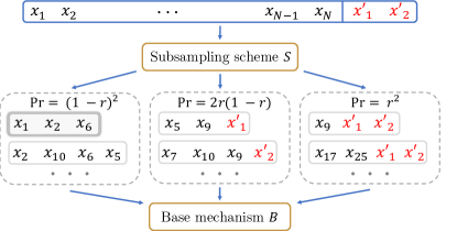
Figure 1: A dataset is processed by sampling a single variable-sized batch (e.g., the highlighted one), which includes each element with i.i.d. probability $r$, and then applying a differentially private “base mechanism”. For small $r$, it is unlikely to include a single ($\Pr=2r(1-r)$) or even both ($\Pr=r^{2}$) elements from an inserted group $\{x_{1}^{\prime},x_{2}^{\prime}\}$. This strengthens the privacy guarantees that can be provided to the group $\{x_{1}^{\prime},x_{2}^{\prime}\}$ by the overall subsampled mechanism.

Overall, our main contributions are that we

• provide the first general framework for deriving tight subsampling guarantees for a privacy accountant,

• derive novel, tight Rényi-DP guarantees under the traditional insertion/removal and substitution relations,

• and demonstrate the benefit of analyzing group privacy and amplification by subsampling jointly.

On a higher level, we can answer our original research question about the benefit of jointly studying different properties of differential privacy in the positive. This joint study thus presents a promising direction for future research.

2 Background and Preliminaries

We consider the same general setting as (Balle et al., 2018), but from a Rényi-DP and group privacy perspective. Specifically, we consider some dataset space ${\mathbb{X}}$. This space can be, for example, the powerset ${\mathbb{X}}=\mathcal{P}({\mathbb{A}})$ of some set ${\mathbb{A}}$. But the elements of ${\mathbb{X}}$ can also be graphs, sequences, or any other data collection. We further consider a measurable output space $({\mathbb{Z}},\mathcal{Z})$, such as the space of model gradients or class labels. Finally, we assume the existence of some measure $\lambda$ on the output space, such as the Lebesgue measure for continuous ${\mathbb{Z}}$ or the counting measure $\#$ for discrete ${\mathbb{Z}}$.

2.1 Rényi Differential Privacy

The idea of differential privacy is that one can map from ${\mathbb{X}}$ to $({\mathbb{Z}},\mathcal{Z})$ in a privacy-preserving manner via random functions, typically referred to as mechanisms.

Definition 2.1.

A random function $M$ from ${\mathbb{X}}$ to $({\mathbb{Z}},\mathcal{Z})$ is a function $M:\Omega\times{\mathbb{X}}\rightarrow{\mathbb{Z}}$, where $(\Omega,\mathcal{F},P)$ is some probability space and all $M_{x}:\omega\mapsto M(\omega,x)$ are measurable.

We assume for all mechanisms $M$ that the distribution of each $M_{x}$ is absolutely continuous w.r.t. output measure $\lambda$, i.e., $\forall x\in{\mathbb{X}}:P_{M_{x}}\ll\lambda$, and write $m_{x}$ for the corresponding Radon–Nikodym derivatives $dP_{M_{x}}\mathbin{/}d\lambda$. For example, when the output space $({\mathbb{Z}},\mathcal{Z})$ is continuous and $\lambda$ is the Lebesgue measure, then $m_{x}$ is the density of $P_{M_{x}}$.

Specifically, mechanisms are meant to preserve privacy w.r.t. small dataset modifications. What constitutes a small modification is described by a symmetric neighboring relation $\simeq_{\mathbb{X}}$ on ${\mathbb{X}}$. When ${\mathbb{X}}$ is composed of sets, two particulary important relations are insertion/removal and substitution.

Definition 2.2.

When ${\mathbb{X}}\subseteq\mathcal{P}({\mathbb{A}})$ for some set ${\mathbb{A}}$, the insertion/removal relation is $\simeq_{\pm,{\mathbb{X}}}=\{(x,x^{\prime})\in{\mathbb{X}}^{2}\mid x\subset x^{\prime}\land|x^{\prime}|=|x|+1\}\cup\{(x,x^{\prime})\in{\mathbb{X}}^{2}\mid x\supset x^{\prime}\land|x^{\prime}|=|x|-1\}$.

Definition 2.3.

When ${\mathbb{X}}\subseteq\mathcal{P}({\mathbb{A}})$ for some set ${\mathbb{A}}$, the substitution relation is $\simeq_{\Delta,{\mathbb{X}}}=\{(x,x^{\prime})\in{\mathbb{X}}^{2}\mid|x|=|x^{\prime}|\land|\Delta(x,x^{\prime})|=2\}$, with symmetric difference $\Delta$.

In the following, we always assume that the elements of ${\mathbb{X}}$ are sets when discussing $\simeq_{\pm,{\mathbb{X}}}$ or $\simeq_{\Delta,{\mathbb{X}}}$.

Privacy is preserved when the distributions of all $M_{x}$, $M_{x^{\prime}}$ with $x\simeq_{\mathbb{X}}x^{\prime}$ are similar to each other. In Rényi-DP, similarity between distributions is quantified via Rényi divergence:

Definition 2.4.

For $\alpha>1$, a random function $M$ from ${\mathbb{X}}$ to $({\mathbb{Z}},\mathcal{Z})$ is $(\alpha,\epsilon)$-RDP w.r.t. neighboring relation $\simeq_{\mathbb{X}}$ if $\forall x\simeq_{\mathbb{X}}x^{\prime}:\log(\Psi_{\alpha}(m_{x}||m_{x^{\prime}}))\mathbin{/}(\alpha-1)\leq\epsilon$, where

$$\Psi_{\alpha}(m_{x}||m_{x^{\prime}})=\int_{\mathbb{Z}}m_{x}^{\alpha}(z)m_{x^{\prime}}^{1-\alpha}(z)\ d\lambda(z).$$ (1)

In the following, we focus on integral $\Psi_{\alpha}$ instead of divergence $\log(\Psi_{\alpha}(m_{x}||m_{x^{\prime}}))\mathbin{/}(\alpha-1)$ to avoid clutter.

2.2 Subsampled Mechanisms

For our discussion of amplification, we additionally consider some measurable space of batches $({\mathbb{Y}},\mathcal{Y})$, which is composed of objects like subsets or subgraphs, and equipped with a neighboring relation $\simeq_{\mathbb{Y}}$. These batches are constructed from datasets in ${\mathbb{X}}$ via subsampling schemes.

Definition 2.5.

A subsampling scheme $S$ is a random function from dataset space ${\mathbb{X}}$ to batch space $({\mathbb{Y}},\mathcal{Y})$.

Given a dataset $x\in{\mathbb{X}}$, we write $P_{S_{x}}$ for the subsampling distribution over batches. When the datasets ${\mathbb{X}}$ are sets and the batches ${\mathbb{Y}}$ are their subsets, two particularly useful schemes are Poisson subsampling (recall Fig. 1) and subsampling without replacement. They are absolutely continuous w.r.t. counting measure $\#$ and we write $s_{x}$ for $dP_{S_{x}}\mathbin{/}d\#$.

Definition 2.6.

For ${\mathbb{X}}\subseteq\mathcal{P}({\mathbb{A}})$, ${\mathbb{Y}}=\{y\subseteq x\mid x\in{\mathbb{X}}\}$, $\mathcal{Y}=\mathcal{P}({\mathbb{Y}})$, and finite set ${\mathbb{A}}$, Poisson subsampling with rate $r\in[0,1]$ is defined by $s_{x}(y)=\mathbbm{1}[y\subseteq x]\cdot r^{|y|}(1-r)^{|x|-|y|}$.

Definition 2.7.

For ${\mathbb{X}}\subseteq\{x\in\mathcal{P}({\mathbb{A}})\mid|x|>q\}$, ${\mathbb{Y}}=\{y\subseteq x\mid x\in{\mathbb{X}},|y|=q\}$, $\mathcal{Y}=\mathcal{P}({\mathbb{Y}})$ and finite set ${\mathbb{A}}$, subsampling without replacement and with batch size $q$ is defined by $s_{x}(y)=\mathbbm{1}[y\subseteq x]\cdot\mathbbm{1}[|y|=q]\cdot\binom{|x|}{q}^{-1}$.

Unless otherwise specified, we assume ${\mathbb{X}}$ and $({\mathbb{Y}},\mathcal{Y})$ to be defined as in Definition 2.6 and Definition 2.7 when discussing the respective subsampling schemes.

The core idea of amplification by subsampling is to compose a subsampling scheme $S$ with a base mechanism $B$ to obtain a subsampled mechanism $M=B\circ S$.

Definition 2.8.

A base mechanism $B$ is a random function from batch space $({\mathbb{Y}},\mathcal{Y})$ to output space $({\mathbb{Z}},\mathcal{Z})$.

We assume the distributions of all $B_{y}\in{\mathbb{Z}}$ to be absolutely continuous w.r.t. output measure $\lambda$ and write $b_{y}$ for $dP_{B_{y}}\mathbin{/}d\lambda$. Hence, the distribution $P_{M_{x}}$ of subsampled mechanism $M=B\circ S$ applied to dataset $x$ is a mixture with

$$m_{x}(z)=\int_{\mathbb{Y}}b_{y}(z)\ dP_{S_{x}}(y).$$ (2)

There is one component per batch $y$ from batch space ${\mathbb{Y}}$, and the weights depend on subsampling distribution $P_{S_{x}}$.

2.3 Group Privacy and Induced Distance

Our goal is to derive strong guarantees for the simultaneous insertion or removal of $K\in{\mathbb{N}}$ elements. This is a special case of datasets with induced distance $K$.

Definition 2.9.

The distance $d_{\mathbb{X}}(x,x^{\prime})$ induced by relation $\simeq_{\mathbb{X}}$ is the length of the shortest sequence $x_{1},\dots,x_{K-1}$ such that $x\simeq_{\mathbb{X}}x_{1}$, $\forall k:x_{k}\simeq_{\mathbb{X}}x_{k+1}$, and $x_{K-1}\simeq x^{\prime}$.

Privacy guarantees for datasets with induced distance $K$ are provided by Proposition 2 in (Mironov, 2017):

Proposition 2.10.

If mechanism $M$ is $(\alpha,\epsilon)$-RDP w.r.t. $\simeq_{\mathbb{X}}$, then it is $(\alpha\mathbin{/}K,\epsilon\cdot 3^{\log_{2}(K)})$-RDP w.r.t. $\{(x,x^{\prime})\in{\mathbb{X}}^{2}\mid d_{\mathbb{X}}(x,x^{\prime})=K\}$ for any $K\in\{2^{C}\mid C\in{\mathbb{N}}_{0}\land 2^{C+1}\leq\alpha\}$.

For our experimental evaluation, we use a tighter guarantee based on Corollary 4 of (Mironov, 2017) (see Section B.1).

3 Unified Amplification by Subsampling

To derive tight group privacy amplification guarantees for Rényi-DP, we need a principled way of bounding the Rényi divergence between mixtures induced by subsampling schemes. Looking at the mixture integral Eq. 2, we identify two challenges: Firstly, there is a large number of mixture components, with one $b_{y}:{\mathbb{Z}}\rightarrow{\mathbb{R}}_{+}$ per batch $y$ from batch space $({\mathbb{Y}},\mathcal{Y})$. Secondly, we may not have an analytic formula for the mixture components, such as the density of noisy model gradients given a batch $y$.

As a starting point, let us consider the joint convexity of $\Psi_{\alpha}$ from Eq. 1 in the space of functions ${\mathbb{Z}}\rightarrow{\mathbb{R}}_{+}$, which immediately follows from joint convexity of $x,y\mapsto x^{\alpha}y^{1-\alpha}$ (Wang et al., 2019) and linearity of integration.

Lemma 3.1.

For arbitrary $\alpha>1$, $w\in[0,1]$, and functions $f_{1},f_{2},f_{3},f_{4}:{\mathbb{Z}}\rightarrow{\mathbb{R}}_{+}$, $\Psi_{\alpha}(wf_{1}+(1-w)f_{3}||wf_{2}+(1-w)f_{4})\leq w\Psi_{\alpha}(f_{1}||f_{2})+(1-w)\Psi_{\alpha}(f_{3}||f_{4})$.

In our case, the functions can be base mechanism densities $b_{y}$ with different $y\in{\mathbb{Y}}$, and the weights can depend on subsampling distributions. Thus, we could potentially use Lemma E.1 to decompose our divergence between mixtures. However, this would require mixtures with identical weights. This is generally not the case, since subsampling distributions $P_{S_{x}}$ and $P_{S_{x^{\prime}}}$ depend on datasets $x\neq x^{\prime}$.

To still leverage the joint convexity of $\Psi_{\alpha}(m_{x}||m_{x^{\prime}})$, we want to rewrite $m_{x}$ and $m_{x^{\prime}}$ as mixtures with identical weights. This is exactly what is offered by couplings between probability measures.

Definition 3.2.

A coupling between probability measures $P_{1},\dots,P_{N}$ on space $({\mathbb{Y}},\mathcal{Y})$ is a probability measure $\Gamma$ on product space $({\mathbb{Y}},\mathcal{Y})^{N}$, where the $n$th marginal is $P_{n}$, i.e., $\Gamma\circ\pi_{n}^{-1}=P_{n}$ with projection $\pi_{n}({\bm{y}})={y}_{n}$.

Intuitively, when considering a coupling between two distributions $P_{1}$, $P_{2}$, the value $\Gamma(T,R)$ specifies for all events $T,R\in\mathcal{Y}$ how much probability should be transported from $P_{1}(T)$ to $P_{2}(R)$ to transform $P_{1}$ into $P_{2}$.

Given a valid coupling $\Gamma$ between subsampling distributions $P_{S_{x}}$ and $P_{S_{x^{\prime}}}$, we can use projection $\pi_{1}$ and change of variables to rewrite $m_{x}$ as $\int_{{\mathbb{Y}}^{2}}b_{y_{\pi_{1}({\bm{y}})}}\ d\Gamma({\bm{y}})$. Similarly, we can rewrite $m_{x^{\prime}}$ as $\int_{{\mathbb{Y}}^{2}}b_{y_{\pi_{2}({\bm{y}})}}\ d\Gamma({\bm{y}})$. Now, both $m_{x}$ and $m_{x^{\prime}}$ are mixtures, with one component per pair of batches in ${\mathbb{Y}}^{2}$. Since they have identical weights induced by coupling $\Gamma$, we can finally apply Lemma 3.1 (full proof in Appendix C):

Theorem 3.3.

Consider a subsampled mechanism $M=B\circ S$, and an arbitrary coupling $\Gamma$ between subsampling distributions $P_{S_{x}}$ and $P_{S_{x^{\prime}}}$. Then, for all $\alpha>1$,

$$\Psi_{\alpha}(m_{x}||m_{x^{\prime}})\leq\int_{{\mathbb{Y}}^{2}}c_{\alpha}(y^{(1)},y^{(2)})\ d\Gamma((y^{(1)},y^{(2)}))$$ (3)

with cost function $c_{\alpha}(y^{(1)},y^{(2)})=\Psi_{\alpha}(b_{y^{(1)}}||b_{y^{(2)}})$.

We write $y^{(1)}$ instead of $y_{1}$ to simplify later notations. While every coupling $\Gamma$ yields a valid upper bound, the guarantees can be tightened by finding a coupling $\Gamma^{*}$ that minimizes the r.h.s. of Eq. 3. We thus have an optimal transport problem, where the cost of transporting probability from batch $y^{(1)}$ to batch $y^{(2)}$ depends on the divergence of base mechanism densities $b_{{y}^{(1)}}$ and $b_{{y}^{(1)}}$.

Theorem 3.3 yields valid Rényi-DP guarantees for arbitrary base mechanisms and subsampling schemes. But, as we demonstrate in Section A.2, Theorem 3.3 is loose for subsampling without replacement, even when using an optimal coupling $\Gamma^{*}$. This can be intuitively explained as follows: Theorem 3.3 is obtained by recursively splitting $m_{x}$ and $m_{x^{\prime}}$ into pairs of mixtures and upper-bounding their corresponding divergences using Lemma 3.1, until one obtains divergences between individual components. These component divergences may not be sufficiently informative to accurately capture the overall mixture divergence.

As a solution to this problem, we propose to limit the recursion depth to which Lemma 3.1 is applied by defining an optimal transport problem between multiple subsampling distributions conditioned on different events (proof in Appendix C). For this, recall that $\mathcal{Y}$ is the $\sigma$-algebra of batch space $({\mathbb{Y}},\mathcal{Y})$, and that $P(T\mid R)=P(T\cap R)\mathbin{/}P(R)$.

Theorem 3.4.

Consider a subsampled mechanism $M=B\circ S$. Further consider two disjoint partitionings $\bigcup_{i=1}^{I}A_{i}={\mathbb{Y}}$ and $\bigcup_{j=1}^{J}E_{j}={\mathbb{Y}}$ such that all $A_{i},E_{j}$ are in $\mathcal{Y}$ and have non-zero measure under $S_{x}$ and $S_{x^{\prime}}$, respectively. Let $\Gamma$ be an arbitrary coupling between $P_{S_{x}}(\cdot\mid A_{1}),\dots,P_{S_{x}}(\cdot\mid A_{I}),P_{S_{x^{\prime}}}(\cdot\mid E_{1}),\dots,P_{S_{x^{\prime}}}(\cdot\mid E_{J})$. Then, for all $\alpha>1$,

$$\Psi_{\alpha}(m_{x}||m_{x^{\prime}})\leq\int_{{\mathbb{Y}}^{I+J}}c_{\alpha}({\bm{y}}^{(1)},{\bm{y}}^{(2)})\ d\Gamma(({\bm{y}}^{(1)},{\bm{y}}^{(2)})),$$

with $c:{\mathbb{Y}}^{I}\times{\mathbb{Y}}^{J}\rightarrow{\mathbb{R}}_{+}$ and $c_{\alpha}({\bm{y}}^{(1)},{\bm{y}}^{(2)})$ defined as

$$\Psi_{\alpha}\left(\sum_{i=1}^{I}b_{{y}^{(1)}_{i}}\cdot P_{S_{x}}(A_{i})||\sum_{j=1}^{J}b_{{y}_{j}^{(2)}}\cdot P_{S_{x^{\prime}}}(E_{j})\right).$$ (4)

Note that we now have a simultaneous coupling between $I+J$ distributions, one per event. Unlike before, Lemma 3.1 is only applied until one is left with pairs of small mixtures that have $I$ and $J$ components, respectively. The special case of using a single event, i.e., $A_{1}={\mathbb{Y}},E_{1}={\mathbb{Y}}$, corresponds to Theorem 3.3, i.e., recursing to maximum depth. The special case of using one event per batch (for finite, discrete ${\mathbb{Y}}$) is equivalent to not applying Lemma 3.1 at all.

To summarize, we have reduced the broad problem of bounding the Rényi divergence between mixtures to the canonical problem of optimal transport between multiple conditional distributions. However, there are two open problems: Evaluating the cost function and designing an optimal coupling.

Cost Function Bound. As discussed earlier, we may not have an analytic expression for every base mechanism distribution $B_{y}$, which would prevents us from evaluating cost function $c$ defined in Eq. 4. We thus propose to upper-bound $c$ via a straight-forward approach that is inherent to differential privacy: Considering worst-case combinations of base mechanism inputs (proof in Appendix C).

Proposition 3.5.

Consider arbitrary ${\bm{y}}^{(1)}\in{\mathbb{Y}}^{I},{\bm{y}}^{(2)}\in{\mathbb{Y}}^{J}$, and cost function $c$ defined in Eq. 4. Let $d_{\mathbb{Y}}$ be the distance induced by $\simeq_{\mathbb{Y}}$. Then, $c_{\alpha}({\bm{y}}^{(1)},{\bm{y}}^{(2)})\leq\hat{c}_{\alpha}({\bm{y}}^{(1)},{\bm{y}}^{(2)})$, with

$$\hat{c}_{\alpha}({\bm{y}}^{(1)},{\bm{y}}^{(2)})=\max_{\hat{{\bm{y}}}^{(1)},\hat{{\bm{y}}}^{(2)}}c_{\alpha}(\hat{{\bm{y}}}^{(1)},\hat{{\bm{y}}}^{(2)})$$ (5)

subject to $\forall k,l,t,u:d_{\mathbb{Y}}(\hat{{y}}^{(k)}_{t},\hat{{y}}^{(l)}_{u})\leq d_{\mathbb{Y}}({y}^{(k)}_{t},{y}^{(l)}_{u})$ and $\hat{{\bm{y}}}^{(1)}\in{\mathbb{Y}}^{I},\hat{{\bm{y}}}^{(2)}\in{\mathbb{Y}}^{J}$.

Note that the worst-case tuple $(\hat{{\bm{y}}}^{(1)},\hat{{\bm{y}}}^{(2)})\in{\mathbb{Y}}^{I+J}$ depends on $({\bm{y}}^{(1)},{\bm{y}}^{(2)})\in{\mathbb{Y}}^{I+J}$ through the pairwise distances of its elements. As we demonstrate in Sections 3.1 and 4, the upper bound $\hat{c}$ can often be evaluated using high-level information about $B$, such as its sensitivity, i.e., Lipschitzness.

Sufficient Optimality Condition. While every valid coupling $\Gamma$ yields a valid upper bound in Theorem 3.4, this bound can be tightened by designing an optimal coupling $\Gamma^{*}$. To inform this design, we generalize the notion of distance-compatible couplings proposed in (Balle et al., 2018) to an arbitrary number of distributions. Essentially, a $d_{\mathbb{Y}}$-compatible coupling only assigns probability to tuples of batches ${\bm{y}}$ when all pairs ${y}_{i},{y}_{j}$ have the smallest possible distance to ${y}_{1}$ and to each other while still being in the support of their respective marginal distributions. In Appendix D, we prove that $d_{\mathbb{Y}}$-compatibility is sufficient for optimality, and show that the optimal value has a canonical form whenever a $d_{\mathbb{Y}}$-compatible couplings exists. We found that such couplings can be constructed to derive all discussed amplification by subsampling guarantees.

3.1 Existing Amplification by Subsampling Guarantees

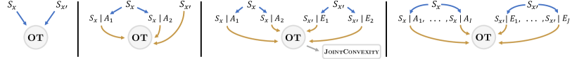
(a)

(b)

(c)

(d)

Figure 2: Existing guarantees (a) (Daigavane et al., 2022), (b) (Mironov et al., 2019; Zhu & Wang, 2019), and (c) (Wang et al., 2019) can be derived from (d) our proposed framework. Guarantee (c) results from upper-bounding the optimal transport value via joint convexity. In (b-c), events $A_{i}$ and $E_{j}$ indicate the presence of inserted or substituted elements.

Now that we have a tractable upper bound on our cost function, and have a heuristic for designing optimal couplings, we can demonstrate the utility of Theorem 3.4 by showing that it can recover the amplification guarantees in (Wang et al., 2019; Zhu & Wang, 2019; Mironov et al., 2019; Daigavane et al., 2022). As shown in (see Fig. 2), this only requires conditioning on few, simple events. Here, we focus on subsampling without replacement and substitution (Wang et al., 2019). We derive the other guarantees in Appendix E.

Theorem 3.6.

Let $M=B\circ S$ be a subsampled mechanism, where $S$ is subsampling without replacement with batch size $q$. Let $\simeq_{\mathbb{Y}}$ be the substitution relation $\simeq_{\Delta,{\mathbb{Y}}}$. Then, for $\alpha>1$ and all $x\simeq_{\Delta,{\mathbb{X}}}x^{\prime}$ of size $N$, $\Psi_{\alpha}(m_{x}||m_{x^{\prime}})$ is l.e.q.

$$\max_{y_{1},y_{2},y_{3},y_{4}}\Psi_{\alpha}((1-w)\cdot b_{y_{1}}+w\cdot b_{y_{2}}||(1-w)\cdot b_{y_{3}}+w\cdot b_{y_{4}})$$

subject to $y_{1}=y_{3}$, $d_{\Delta,{\mathbb{Y}}}(y_{1},y_{2})\leq 1$, $d_{\Delta,{\mathbb{Y}}}(y_{1},y_{4})\leq 1$, $d_{\Delta,{\mathbb{Y}}}(y_{2},y_{4})\leq 1$, and with $w=q\mathbin{/}N$.

Proof sketch.

Since $x\simeq_{\Delta,{\mathbb{X}}}x^{\prime}$, there must be some $a\in x$, $a^{\prime}\in x^{\prime}$ such that $x^{\prime}=x\setminus\{a\}\cup\{a^{\prime}\}$. We define $A_{1}$ and $E_{1}$ to be the event that neither $a$ nor $a^{\prime}$ is sampled, i.e., $A_{1}=E_{1}=\{y\in{\mathbb{Y}}\mid y\cap\{a,a^{\prime}\}=\varnothing\}$, and $A_{2}$ and $E_{2}$ be their complements $\overline{A_{1}}$ and $\overline{E_{1}}$. Constructing a $d_{\mathbb{Y}}$-compatible coupling for the resultant conditional subsampling distribution yields the result. ∎

This bound is different from that of Wang et al. (2019) (cf. Proposition E.2). We can recover their result by bounding Theorem 3.6 once more via joint convexity (see Section E.1). However, we can obtain tighter guarantees by evaluating Theorem 3.6 exactly for specific mechanisms, such as randomized response:

Theorem 3.7.

Let $B$ be the randomized response mechanism $|f-(1-V)|$ with $f:{\mathbb{Y}}\rightarrow\{0,1\}$, $V\sim\mathrm{Bernoulli}(\theta)$, and true response probability $\theta\in[0,1]$. Let $S$ be subsampling without replacement with batch size $q$. Then, for $\alpha>1$ and all $x\simeq_{\Delta,{\mathbb{X}}}x^{\prime}$ of size $N$, $\Psi_{\alpha}(m_{x}||m_{x^{\prime}})$ is l.e.q.

$$\max_{\tau_{1},\tau_{2},\tau_{4}}\sum_{z=0}^{1}\frac{((1-w)|z-\tau_{1}|+w|z-\tau_{2}|)^{\alpha}}{((1-w)|z-\tau_{1}|+w|z-\tau_{4}|)^{\alpha-1}}$$

subject to $\tau_{1},\tau_{2},\tau_{4}\in\{\theta,1-\theta\}$ and with $w=q\mathbin{/}N$.

Tightness. Theorem 3.7 is tight, i.e., it is not possible to derive stronger RDP guarantees without additional information about ${\mathbb{X}}$ and $f$ (see Section F.1). As we demonstrate in Section 6, Theorem 3.7 offers significantly stronger guarantee than the best known bound from (Wang et al., 2019).

3.2 Novel Amplification by Subsampling Guarantees

Beyond recovering and improving upon known results, our framework also lets us derive entirely new guarantees for Rényi-DP w.r.t. the traditional $\simeq_{\pm}$ and $\simeq_{\Delta}$ relations. In Section F.2, we demonstrate that one can prove amplification w.r.t. dataset relation $\simeq_{\Delta,{\mathbb{X}}}$ even when the base mechanisms is only known to be differentially private w.r.t.  batch relation $\simeq_{\pm,{\mathbb{Y}}}$. Such “hybrid relations” (Balle et al., 2018) may be particularly useful when ${\mathbb{X}}$ and ${\mathbb{Y}}$ are entirely different spaces. In Section F.3, we consider subsampling without replacement and $\simeq_{\pm}$, which enables Rényi-DP accounting for noisy stochastic gradient descent with fixed batch sizes.

4 Group Privacy Amplification

Now that we have a general framework for amplification by subsampling in Rényi-DP, we can apply it to our original goal of deriving (tight) group privacy amplification guarantees. In the following, we focus on the Poisson subsampling scheme (recall Fig. 1). We want to provide guarantees for the insertion or removal of a group of size $K$, i.e., neighboring relation $\simeq_{\pm K,{\mathbb{X}}}=\{(x,x^{\prime})\in{\mathbb{X}}^{2}\mid x\subset x^{\prime}\land|x^{\prime}|=|x|+K\}\cup\{(x,x^{\prime})\in{\mathbb{X}}^{2}\mid x\supset x^{\prime}\land|x^{\prime}|=|x|-K\}.$

In Section E.2, we demonstrate that Zhu & Wang (2019)’s tight guarantees for $K=1$ can be obtained by conditioning on the presence of the single inserted / removed element and constructing a $d_{\mathbb{Y}}$-compatible coupling. A natural generalization for $K>1$ is to condition on the number of group elements that appear in a batch. Constructing a $d_{\mathbb{Y}}$-compatible coupling between the resultant $K+2$ conditional distributions (see proof in Section G.1) yields:

Theorem 4.1.

Let $M=B\circ S$ be a subsampled mechanism, where $S$ is Poisson subsampling with rate $r$. Let $\simeq_{\mathbb{Y}}$ be the insertion/removal relation $\simeq_{\pm,{\mathbb{Y}}}$. Then, for $\alpha>1$ and all $x\simeq_{\pm K,{\mathbb{X}}}x^{\prime}$, $\Psi_{\alpha}(m_{x}||m_{x^{\prime}})$ is l.e.q. the maximum of

$$\max\left(\Psi_{\alpha}(\sum_{i=1}^{K+1}w_{i}b_{y_{i}}||b_{y_{K+2}}),\Psi_{\alpha}(b_{y_{K+2}}||\sum_{j=1}^{K+1}w_{j}b_{y_{j}})\right)$$

subject to ${\bm{y}}\in{\mathbb{Y}}^{K+2}$, $y_{1}=y_{K+2}$, $\forall t,u<K+2:d_{\mathbb{Y}}(y_{t},y_{u})\leq|t-u|$, and with $w_{i}=\mathrm{Binomial}(i-1\mid K,r)$.

Next, we can evaluate the term in Theorem 4.1 for specific base mechanisms, such as the Gaussian mechanism:

Theorem 4.2.

Let $M=B\circ S$ be a subsampled mechanism, where $S$ is Poisson subsampling with rate $r$, and $B$ is the Gaussian mechanism $f+V$ with $f:{\mathbb{Y}}\rightarrow{\mathbb{R}}^{D}$ and $V\sim\mathcal{N}({\bm{\mu}},\sigma^{2}{\bm{I}}_{D})$, with mean ${\bm{\mu}}\in{\mathbb{R}}^{D}$ and diagonal covariance matrix $\sigma^{2}{\bm{I}}_{D}\in{\mathbb{R}}_{+}^{D\times D}$. Define the $\ell_{2}$-sensitivity $L_{2}=\max_{y\simeq_{\pm,{\mathbb{Y}}}y^{\prime}}||f(y)-f(y^{\prime})||_{2}$. Then, for $\alpha>1$ and all $x\simeq_{\pm K,{\mathbb{X}}}x^{\prime}$, $\Psi_{\alpha}(m_{x}||m_{x^{\prime}})$ is l.e.q.

$$\max\left(\Psi_{\alpha}(\sum_{i=1}^{K+1}w_{i}d_{i}||d_{1}),\Psi_{\alpha}(d_{1}||\sum_{j=1}^{K+1}w_{j}d_{j})\right)$$

with $w_{i}=\mathrm{Binomial}(i-1\mid K,r)$ and univariate normal densities $d_{i}=\mathcal{N}(\cdot\mid(i-1),\sigma^{2}\mathbin{/}L_{2}^{2}{\bm{I}}_{1})$.

In Sections G.3 and H, we rigorously prove that Gaussians with collinear and equidistant means maximize the two $\Psi_{\alpha}$ terms in Theorem 4.1. This allows for a reduction to univariate Gaussian distributions via marginalization. Both terms can be evaluated via univariate numerical integration, similar to (Abadi et al., 2016). The first term can also be evaluated via multinomial expansion. In Section G.2 we derive a similar guarantee for randomized response.

Tightness. Our group privacy guarantees for subsampled Gaussian and randomized response mechanisms are tight (proofs in Sections G.3 and G.2): One cannot derive stronger Rényi-DP guarantees without additional information about dataset space ${\mathbb{X}}$ or the underlying function $f$.

5 Limitations

While our proposed framework unifies and generalizes prior work, there is room for further generalization: Future work may want to (a) make more general use of the law of total expectation to lift our restriction to finite sets of events in Theorem 3.4, and (b) prove convexity for a more general definition of Rényi divergence than Eq. 1, so that we do not have to assume absolutely continuity w.r.t. output measure $\lambda$. Furthermore, even though we found conditioning on the presence of number of modified elements to be sufficient for all considered scenarios, it would be desirable to develop an automated procedure for selecting events in Theorem 3.4. Maximal couplings fulfill this purpose for single-element relations in (Balle et al., 2018), but only yield pairs of conditional distributions. Finally, while tight Rényi-DP guarantees can exactly characterize a mechanism’s privacy leakage (Sommer et al., 2019), the known conversion formulae to $(\epsilon,\delta)$-DP are lossy (Zhu et al., 2022). Future work should thus generalize our framework to other accountants.

6 Experimental Evaluation

Figure 3: Randomized response with varying true response probability $\theta$ under subsampling without replacement with batch-to-dataset ratio $q\mathbin{/}N=0.001$. Theorem 3.7 significantly improves upon the baseline for a wide range of $\alpha$.

The following experiments serve two purposes: Firstly, we want to demonstrate the effectiveness of our unified amplification by subsampling framework, in which we derive guarantees for subsampled Rényi-DP mechanisms via optimal transport between multiple conditional subsampling distributions. Secondly, we want to verify that the tight group privacy amplification guarantees derived in Section 4 are stronger than a combination of known group privacy and amplification bounds for Rényi-DP.

Whenever we evaluate prior work (i.e., (Wang et al., 2019) or (Zhu & Wang, 2019)) in the context of group privacy, we imply that this method is combined with the group privacy bound from Section B.1. Further details on the experimental setup are provided in Appendix B.

Subsampling Without Replacement and Randomized Response. One of the novel results we derived in Appendix F is a tight bound for subsampling without replacement applied to randomized response mechanisms under the substitution relation $\simeq_{\Delta}$. Fig. 3 compares this result to the best known bound derived by (Wang et al., 2019) for varying true response probabilities $\theta\in\{0.6,0.75,0.9\}$ and ratio $q\mathbin{/}N=0.001$, where $q$ is the batch size and $N$ the dataset size. As shown in Fig. 3, Theorem 3.7 consistently improves upon the baseline for a wide range of $\alpha\leq 10^{4}$. In Section A.1 we verify that this result is consistent across various $q\mathbin{/}N$ ratios, thus demonstrating the usefulness of our optimal transport based framework.

(a) $r=0.2$

(b) $r=0.1$

(c) $r=0.001$

Figure 4: Randomized response ($\theta=0.75$) under Poisson subsampling with varying subsampling rates $r$ and group sizes. The tight guarantees can be significantly stronger, but the baseline is a good upper bound for small subsampling rate.

Benefit of Conditioning. A natural question is whether it is necessary to consider conditional distributions in Theorem 3.4, or if the simpler optimal transport problem from Theorem 3.3, which we have used to recover the amplification guarantees of (Daigavane et al., 2022), is sufficient. To answer this question, we compare Proposition E.5 to (Wang et al., 2019) for subsampling without replacement, Gaussian mechanisms and $\simeq_{\Delta}$ Section A.2. We find that, in the group privacy setting, there are ranges of parameters such that Proposition E.5 improves upon the baseline. But it is not sufficient for consistently outperforming it. Interestingly, it captures the impossibility of including more than $1$ group element in a batch of size $1$, unlike the baseline.

Randomized Response Group Privacy. Next, we turn to our objective of evaluating our group privacy amplification guarantees, beginning with randomized response ($\theta=0.75$), subsampling rates $r\in\{0.2,0.1,0.001\}$, and group sizes in $\{2,4,8\}$ (see Theorem G.1). As shown in Fig. 4, our tight guarantee can outperform the baseline for a wide range of $\alpha\leq 10^{4}$, with the gap being particularly big for large groups. Interestingly, we find that the baseline converges to the tight guarantee as $r$ decreases, which we also observe for various other $\theta\in\{0.6,0.7,0.8,0.9\}$ in Section A.3. Importantly, this is not a deficiency of Theorem G.1. The guarantee is tight and cannot be improved. The baseline is just a good upper bound for small subsampling rates.

Gaussian Mechanism Group Privacy. Next, we consider the Gaussian mechanism ($\sigma=1$) in the same setting. Here, a different interesting pattern emerges: As observed in (Wang et al., 2019; Zhu & Wang, 2019), subsampled Gaussian mechanisms undergo a phase transition from a high-privacy regime to a low-privacy regime at some $\alpha^{*}$ that increases with $\sigma$ and decreases with $r$. As can be inferred from Proposition 2.10, this phase transition bound decreases to $\approx\alpha^{*}\mathbin{/}K$ when using the traditional group privacy property for groups of size $K$. In comparison, our tight analysis lets us delay this phase transition, extending the high-privacy regime to larger $\alpha$. However, when considering highly private base mechanisms (e.g. $\sigma=5$), this extension only makes up a small fraction of the high-privacy range (see Section A.4)

Conversion to $(\epsilon,\delta)$-DP. As we demonstrate in Section A.5, similar patterns emerge when converting from Rényi-DP to $(\epsilon,\delta)$-DP: Our tight bounds can result in a significantly smaller accumulated privacy cost over multiple compositions. But the traditional group privacy property is a good upper bound when amplifying mechanisms that are already very private via small subsampling rates.

(a) $r=0.2$

(b) $r=0.1$

(c) $r=0.001$

Figure 5: Gaussian mechanism ($\sigma=1.0$) under Poisson subsampling with varying subsampling rates $r$ and group sizes. The tight analysis delays the phase transition from a high- to a low-privacy regime.

7 Related Work

Amplification by Subsampling for Rényi-DP. Mironov (2017)’s original work on Rényi-DP, which developed existing moments-based accounting methods (Abadi et al. (2016); Dwork & Rothblum (2016); Bun & Steinke (2016)) into a general notion of moments-based privacy, did not discuss amplification. However, later work derived tight amplification guarantees for Poisson subsampling and insertion / removal (Mironov et al., 2019; Zhu & Wang, 2019), as well as subsampling without replacement and substitution (Wang et al., 2019). Our work shows that each of these results can be derived from the general principle of optimal transport between conditional subsampling distributions.

Amplification by Subsampling for Graph Machine Learning. Group privacy is related to the problem of privacy-preserving training of arbitrary graph neural networks for node-level tasks (Daigavane et al., 2022), where modification of a single node’s features or edges can affect all per-sample gradients within a neighborhood. As we prove in Section E.3, the RDP amplification guarantees in (Daigavane et al., 2022) can be derived via optimal transport without conditioning. But as demonstrated in Section A.2, this approach is not sufficient for consistently outperforming guarantees derived via conditioning. However, it interestingly could provide much stronger guarantees for batch size $1$, by leveraging information about the internals of a subsampled mechanism.

Amplification by Subsampling for $(\epsilon,\delta)$-DP. Using subsampling to strenghten $(\epsilon,\delta)$-DP guarantees has a long history (Kasiviswanathan et al., 2011; Li et al., 2012) particularly in privacy-preserving machine learning (Bassily et al., 2014; Wang et al., 2015; Abadi et al., 2016). Balle et al. (2018) ultimately proposed a general framework for analyzing subsampled $(\epsilon,\delta)$-DP mechanisms via optimal transport. However, they do not consider Rènyi-DP or any other accounting method. And, unlike in Theorem 3.4, they do not define couplings between multiple conditional distributions. They instead use a construction (“advanced joint convexity”) that is specifically tailored to $(\epsilon,\delta)$-DP. Finally, they do not provide amplification guarantees for groups.

Amplification by Subsampling for Other Accountants. Recent works on privacy accounting generally include a discussion of Poisson subsampling and insertion / removal or subsampling without replacement and substitution (Dong et al., 2022; Bu et al., 2020; Koskela et al., 2021; Koskela & Honkela, 2021; Gopi et al., 2021; Ghazi et al., 2022; Alghamdi et al., 2023). Zhu et al. (2022) further consider subsampling without replacement and insertion / removal, and Koskela et al. (2020) analyzes subsampling with replacement. However, they do not provide a generic framework for deriving such results and do not consider group privacy.

Unified Amplification for f-DP. In very recent work, Wang et al. (2023) prove joint concavity of the trade-off functions underlying the f-DP (Dong et al., 2022) accounting method. This enables them to provide amplification guarantees for mixture mechanisms induced by random initialization and shuffling in a unified manner. However, they do not consider amplification by subsampling, and explicitly state that they need to address this problem in future work.

8 Conclusions

The main purpose of this work is to verify that there is a benefit to analyzing multiple properties of differential privacy jointly, such as group privacy and amplification by subsampling. To this end, we developed the first general framework for deriving amplification by subsampling guarantees for a privacy accountant, namely Rényi-DP. Besides our main goal, this optimal transport based approach let us derive tight and novel guarantees, e.g., to tightly analyze subsampling without replacement applied to randomized response and under the insertion / removal relation, as well as to convert privacy guarantees of a base mechanism from one neighboring relation to another. Our experimental evaluation lets us answer our original research question in the positive, since the derived group privacy amplification bounds are not only tight, but can also provide significantly stronger guarantees for practical mechanisms. Thus, two promising directions open up for future work: Firstly, further generalization of our approach, for instance via combination with recently proven concavity properties of f-DP (Wang et al., 2023). Secondly, the joint study of different privacy properties, such as group privacy and amplification by shuffling, or amplification by subsampling and composition.

Broader Impact

By combining group privacy and amplification by subsampling, this research aims to provide stronger privacy guarantees. This can foster the development of more secure and trustworthy AI systems across privacy-sensitive domains.

Appendix A Additional Experiments

A.1 Subsampling Without Replacement and Randomized Response

In Fig. 6, we repeat our experiment from Fig. 3 for a wider range of ratios between dataset size $N$ and batch size $q$. Our novel, tight guarantee for randomized response mechanisms from Theorem 3.7 improves upon the previous best known bound across both high and low true response probabilities $\theta$, as well as small and large ratios $q\mathbin{/}N$. This demonstrates the benefit of analyzing subsampling without replacement via Theorem 3.6, instead of upper-bounding it once more via joint convexity, as is done in (Wang et al., 2019).

A.2 Direct Transport

Next, we evaluate Proposition E.5, which can be derived via Theorem 3.3, i.e. optimal transport without conditioning, for a wide range of dataset sizes, batch sizes, and group sizes (see Fig. 7). Note that, unlike with the guarantees of (Wang et al., 2019), this bound depends on both the dataset size and the batch size, not just their ratio. We make the following observations: For large $\alpha$ Proposition E.5 converges to the baseline. Furthermore, this approach never outperforms the baseline for group size $1$. Neither does it outperform the baseline for ratios $q\mathbin{/}L\in\{0.01,0.001\}$. But, for $q\mathbin{/}L=0.1$, there is a sweet spot of alphas between $10^{1}$ and $10^{2}$ in which it offers stronger guarantees, which further reinforces our claim that there is a benefit to treating group privacy and amplification jointly. Furthermore, we observe that in the case of $q=1$, it outperforms the baseline for large alpha, since it can capture that one cannot possibly include more than one substituted element in a singleton batch.

A.3 Randomized Response Group Privacy

In Fig. 8, we compare our provably tight group privacy guarantee for Poisson subsampled randomized response to the guarantee in (Zhu & Wang, 2019) for a wider range of true response probabilities from $\{0.6,0.7,0.75,0.8,0.9\}$. As we already observed in the main experiment, the tight guarantee offers drastically stronger guarantees for moderate subsampling rates, but the baseline converges to it for small subsampling rates. We further notice that this convergence appears to happen faster when the true response probability is smaller, i.e. the base mechanism is more private. Nevertheless, these results confirm our hypothesis that there is a benefit to studying amplification by subsampling and group privacy jointly.

A.4 Gaussian Mechanism Group Privacy

Next, we compare our provably tight group privacy guarantee for Poisson subsampled Gaussian mechanisms to the guarantee in (Zhu & Wang, 2019) for a wider range of standard deviations $\sigma$ in $\{0.2,0.5,1.0,2.0,5.0\}$. Again, our observations are consistent with the main experiment: When considering the entire range of $\alpha\in[2,10000]$, as shown in Fig. 9, it is hard to notice a difference. However, our tight analysis delays the phase transition from high to low privacy (see Fig. 9). As we shall see in the next experiment, this can have a significant impact on the resultant $({\epsilon},\delta)$ guarantees.

A.5 Conversion to $({\epsilon},\delta)$-DP

Finally, we convert our guarantees to $({\epsilon},\delta)$-pairs using the method from (Balle et al., 2020). We begin with the Gaussian mechanism (see Fig. 12 and subsampling rate $r=0.001$. Our bound offers stronger group privacy guarantees for $\sigma=1.0$, but both results are almost identical We suspect that this is because the phase transition, which our result improves, gets shifted to very high $\alpha$ regions that are not useful for conversion to $({\epsilon},\delta)$-DP. Our observations for randomized response mechanisms (see Fig. 12 are also consistent with earlier observations: For moderate subsampling rates $r=0.1$, our guarantees are stronger, particularly for group size $8$ and large numbers of iterations. But, when decreasing the subsampling rate to $0.001$, both methods are almost identical. Nevertheless, group privacy amplification can demonstrably improve upon a direct combination of independently derived group privacy and amplification guarantees.

(a)          $q\mathbin{/}N=0.01$

(b)          $q\mathbin{/}N=0.1$

(c)          $q\mathbin{/}N=0.2$

(d)          $q\mathbin{/}N=0.5$

Figure 6: Randomized response under subsampling without replacement, with varying true response probability $\theta$ and batch-to-dataset ratio $q\mathbin{/}N$. Theorem 3.7 significantly improves upon the baseline for a wide range of $\alpha$.

(a)          $N=10^{5},q=10^{2}$

(b)          $N=10^{5},q=10^{3}$

(c)          $N=10^{5},q=10^{4}$

(d)          $N=10^{4},q=10^{1}$

(e)          $N=10^{4},q=10^{2}$

(f)          $N=10^{4},q=10^{3}$

(g)          $N=10^{3},q=10^{0}$

(h)          $N=10^{3},q=10^{1}$

(i)          $N=10^{3},q=10^{2}$

Figure 7: Proposition E.5 derived from Theorem 3.3 applied to Gaussian mechanism ($\sigma=5.0$) under sampling without replacement for varying dataset size $N$, batch size $q$, and group size. Except for large batch-to-dataset size ratios and for batch size $1$, it does not improve upon the baseline.

(a)          $r=0.2,\theta=0.9$

(b)          $r=0.1,\theta=0.9$

(c)          $r=0.001,\theta=0.9$

(d)          $r=0.2,\theta=0.8$

(e)          $r=0.1,\theta=0.8$

(f)          $r=0.001,\theta=0.8$

(g)          $r=0.2,\theta=0.75$

(h)          $r=0.1,\theta=0.75$

(i)          $r=0.001,\theta=0.75$

(j)          $r=0.2,\theta=0.7$

(k)          $r=0.1,\theta=0.7$

(l)          $r=0.001,\theta=0.7$

(m)          $r=0.2,\theta=0.6$

(n)          $r=0.1,\theta=0.6$

(o)          $r=0.001,\theta=0.6$

Figure 8: Randomized Response under Poisson subsampling for varying true response probability $\theta$, subsampling rate $r$, and group size. Our method yields stronger privacy guarantees for moderate subsampling rates $r$, but the baseline is a good upper bound for very small $r$.

(a)          $r=0.2,\sigma=0.2$

(b)          $r=0.1,\sigma=0.2$

(c)          $r=0.001,\sigma=0.2$

(d)          $r=0.2,\sigma=0.5$

(e)          $r=0.1,\sigma=0.5$

(f)          $r=0.001,\sigma=0.5$

(g)          $r=0.2,\sigma=1.0$

(h)          $r=0.01,\sigma=1.0$

(i)          $r=0.001,\sigma=1.0$

(j)          $r=0.2,\sigma=2.0$

(k)          $r=0.1,\sigma=2.0$

(l)          $r=0.001,\sigma=2.0$

(m)          $r=0.2,\sigma=5.0$

(n)          $r=0.1,\sigma=5.0$

(o)          $r=0.001,\sigma=5.0$

Figure 9: Gaussian mechanism under Poisson subsampling for varying subsampling rate $r$, standard deviation $\sigma$, and group size. The derived result is identical to the baseline, except for the phase transition from high to low privacy, which is hardly visible.

(a)          $r=0.2,\sigma=0.2$

(b)          $r=0.1,\sigma=0.2$

(c)          $r=0.001,\sigma=0.2$

(d)          $r=0.2,\sigma=0.5$

(e)          $r=0.1,\sigma=0.5$

(f)          $r=0.001,\sigma=0.5$

(g)          $r=0.2,\sigma=1.0$

(h)          $r=0.1,\sigma=1.0$

(i)          $r=0.001,\sigma=1.0$

(j)          $r=0.2,\sigma=2.0$

(k)          $r=0.1,\sigma=2.0$

(l)          $r=0.001,\sigma=2.0$

(m)          $r=0.2,\sigma=5.0$

(n)          $r=0.1,\sigma=5.0$

(o)          $r=0.001,\sigma=5.0$

Figure 10: Zooming in for small RDP orders $\alpha$: Gaussian mechanism under Poisson subsampling for varying subsampling rate $r$, standard deviation $\sigma$, and group size. The tight guarantee delays the phase transition from low to high privacy.

(a) $\sigma=1.0$

(b) $\sigma=5.0$

Figure 11: Conversion to $(\epsilon,\delta$) for the Gaussian mechanism under Poisson subsampling with fixed subsampling rate $r=0.001$.

(a) $r=0.1$

(b) $r=0.001$

Figure 12: Conversion to $(\epsilon,\delta$) for the Randomized Response mechanism $(\theta=0.6)$ under Poisson subsampling with varying subsampling rate $r$

Appendix B Experimental Setup

Baselines. When evaluating the bound of (Wang et al., 2019), we use the tightest of their guarantees, including all extensions from their Lemma 17, Lemma 19, and Theorem 27. When evaluating the bound of (Zhu & Wang, 2019), we use the tight version, which eliminates a factor of $2$. When evaluating Proposition E.5, we do not use the group privacy property, but the bound for $K$-fold substitution proposed for graphs in (Daigavane et al., 2022).

Range of RDP orders. For visualization, we evaluate all guarantees for $121$ equidistant points in $\log$-space between $2$ and $10^{4}$, rounded to the next smaller integer. For conversion to $({\epsilon},\delta)$-DP and visualization of the Gaussian mechanisms group privacy guarantees, we additionally consider $121$ equidistant, continuous points in $\log$-space between $0$ and $10$, as well as integers $\{1,2,3,4,\dots,10^{4}\}$. Note that, for the shown examples with Gaussian mechanisms, the optimal value of $\alpha$ was always in the interior of the considered range of orders.

Numerical integration. For Gaussian mechanisms, we use numerical integration, similar to (Abadi et al., 2016), in the following cases: (a) evaluating the reverse divergence in Theorem 4.2, (b) evaluating the forward divergence in Theorem 4.2 for group size 8, as well as group size $4$ for $\alpha>100$. (c) evaluating any bound for continuous orders We perform this integration via $\tanh$-$\sinh$-quadrature with $50$ digits of decimal precision.

Conversion to ($\epsilon,\delta$)-DP. For conversion to $(\epsilon,\delta)$-DP, we use the method proposed in Theorem $21$ of (Balle et al., 2020), which improves upon the conversion formula from (Mironov, 2017).

B.1 Group Privacy Baseline

Proposition 2.10 provides valid guarantees w.r.t. induced distances $K$ that are powers of $2$. However, it is only an upper bound on the following result from Corollary 4 of (Mironov, 2017): Let $D_{\alpha}$ be $\log(\Psi_{\alpha})\mathbin{/}(\alpha-1)$. Then

$$D_{\alpha}(p||q)\leq\frac{\alpha-\frac{1}{2}}{\alpha-1}D_{2\alpha}(p||r)+\frac{\alpha}{\alpha-1}D_{2\alpha-1}(r||q).$$

We recursively apply this bound $\log_{2}(K)$ times when evaluating the group privacy of our baselines for groups of size $K$.

Appendix C Unified Amplification by Subsampling

C.1 Proof of Theorem 3.3

See 3.3

Proof.

Recall that $m_{x}$ and $m_{x^{\prime}}$ are mixtures with $m_{x}(z)=\int b_{y}(z)\ dP_{S_{x}}(y)$ and $m_{x^{\prime}}(z)=\int b_{y}(z)\ dP_{S_{x^{\prime}}}(y)$. Since $\Gamma$ is a coupling between $P_{S_{x}}$ and $P_{S_{x^{\prime}}}$, we can use the projection $\pi_{n}({\bm{y}})={y}_{n}$ and change of variables to rewrite these mixtures as

$$m_{x}(z)=\int_{\mathbb{Y}}b_{y}(z)\ d\left(\Gamma\circ\pi_{1}^{-1}\right)(y)=\int_{{\mathbb{Y}}^{2}}b_{\pi_{1}({\bm{y}})}(z)\ d\Gamma({\bm{y}})=\int_{{\mathbb{Y}}^{2}}b_{{y}_{1}}(z)\ d\Gamma({\bm{y}}),$$

$$m_{x^{\prime}}(z)=\int_{\mathbb{Y}}b_{y}(z)\ d\left(\Gamma\circ\pi_{2}^{-1}\right)(y)=\int_{{\mathbb{Y}}^{2}}b_{\pi_{2}({\bm{y}})}(z)\ d\Gamma({\bm{y}})=\int_{{\mathbb{Y}}^{2}}b_{{y}_{2}}(z)\ d\Gamma({\bm{y}}).$$

Since $m_{x}(z)$ and $m_{x^{\prime}}(z)$ are now expectations w.r.t. the same measure, we can use the joint convexity of $\Psi_{\alpha}$ (Lemma 3.1) to show $\Psi_{\alpha}(m_{x},m_{x^{\prime}})\leq\int_{{\mathbb{Y}}^{2}}\Phi_{\alpha}(b_{y_{1}}||b_{y_{2}})\ d\Gamma({\bm{y}}).$ ∎

C.2 Proof of Theorem 3.4

See 3.4

Proof.

Using the law of total expectation, linearity of integration, and change of variables with projection $\pi_{n}({\bm{y}})={y}_{n}$ shows that

$$m_{x}(z) =\sum_{i=1}^{I}\left(\int_{\mathbb{Y}}b_{y}(z)\ dP_{S_{x}}(y\mid A_{i})\right)P_{S_{x}}(A_{i})$$

$$=\int_{\mathbb{Y}}\left(\sum_{i=1}^{I}b_{y}(z)\cdot P_{S_{x}}(A_{i})\right)\ dP_{S_{x}}(y\mid A_{i})$$

$$=\int_{{\mathbb{Y}}}\left(\sum_{i=1}^{I}b_{y}(z)\cdot P_{S_{x}}(A_{i})\right)\ d(\Gamma\circ\pi_{i}^{-1})(y)$$

$$=\int_{{\mathbb{Y}}^{I+J}}\left(\sum_{i=1}^{I}b_{y_{i}}(z)\cdot P_{S_{x}}(A_{i})\right)\ d\Gamma({\bm{y}})$$

and

$$m_{x}(z)=\int_{{\mathbb{Y}}^{I+J}}\left(\sum_{j=1}^{J}b_{y_{(j+I)}}(z)\cdot P_{S_{x}}(E_{j})\right)\ d\Gamma({\bm{y}}).$$

Since $m_{x}(z)$ and $m_{x^{\prime}}(z)$ are now expectations w.r.t. the same measure, we can use the joint convexity of $\Psi_{\alpha}$ (Lemma 3.1) to show

$$\Psi_{\alpha}(m_{x}||m_{x^{\prime}})\leq\int_{{\mathbb{Y}}^{I+J}}\Psi_{\alpha}\left(\sum_{i=1}^{I}b_{y_{i}}(z)\cdot P_{S_{x}}(A_{i})||\sum_{j=1}^{J}b_{y_{(j+I)}}(z)\cdot P_{S_{x}}(E_{j})\right)\ d\Gamma({\bm{y}}).$$

A change of indexing via ${\bm{y}}^{(1)}_{i}={\bm{y}}_{i}$ and ${\bm{y}}^{(2)}_{j}={\bm{y}}_{(j+I)}$ concludes our proof. ∎

C.3 Proof of Proposition 3.5

See 3.5

Proof.

The original tuples of batches ${\bm{y}}^{(1)}\in{\mathbb{Y}}^{I}$ and ${\bm{y}}^{(2)}\in{\mathbb{Y}}^{J}$ constitute a feasible solution to the optimization problem, since they fulfill the constraints with equality, i.e., $\forall k,l,t,u:d_{\mathbb{Y}}({y}^{(k)}_{t},{y}^{(l)}_{u})=d_{\mathbb{Y}}({y}^{(k)}_{t},{y}^{(l)}_{u})$. The value of any feasible solution to an optimization problem is l.e.q. its optimal value. ∎

Appendix D Distance-Compatible Couplings of Multiple Distributions

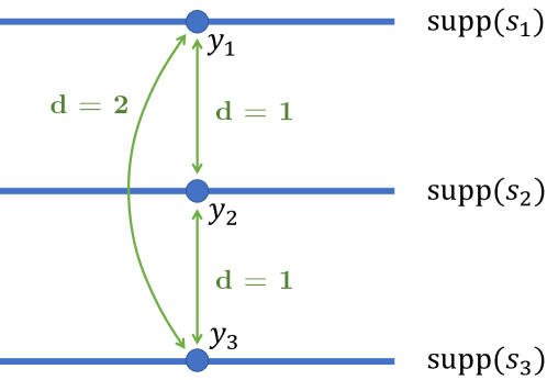
(a) Distance-compatible coupling

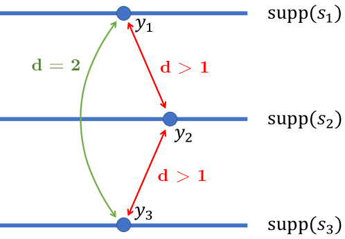
(b) Distance-incompatible coupling

Figure 13: Example of a distance-compatible and a distance-incompatible coupling

In the following, we generalize the notion of distance-compatible couplings proposed in (Balle et al., 2018) from two distributions to an arbitrary number of distributions. This provides a sufficient optimality condition for Theorem 3.4.

As discussed in Section 3, a $d_{\mathbb{Y}}$-compatible coupling between (conditional) subsampling distributions only assigns probability to tuples of batches ${\bm{y}}$ when all pairs ${y}_{i},{y}_{j}$ have the smallest possible distance to ${y}_{1}$ and to each other, while still being in the support of their respective distributions.

To avoid having to make additional assumptions about the topology of batch space $({\mathbb{Y}},\mathcal{Y})$, we will assume that all subsampling schemes have densities and reason about the support of these densities.

Definition D.1.

The set-theoretic support of a function $s:{\mathbb{Y}}\rightarrow{\mathbb{R}}_{+}$ is $\mathrm{supp}(s)=\{y\in{\mathbb{Y}}\mid s(y)>0\}$.

Based on this notion of support, we can define a notion of distance between a batch $y\in{\mathbb{Y}}$ and the support of a density:

Definition D.2.

Consider a distance $d_{\mathbb{Y}}$ induced by a neighboring relation $\simeq_{\mathbb{Y}}$. The distance between an element $y\in{\mathbb{Y}}$ and the support of a function $s:{\mathbb{Y}}\rightarrow{\mathbb{R}}_{+}$ is defined as $d_{\mathbb{Y}}(y,\mathrm{supp}(p))=\min_{y^{\prime}\in\mathrm{supp}(p)}d_{\mathbb{Y}}(y,y^{\prime})$.

Furthermore, we can define a notion of distance between the support of two different densities:

Definition D.3.

Consider a distance $d_{\mathbb{Y}}$ induced by a neighboring relation $\simeq_{\mathbb{Y}}$. The distance between the support of functions $s_{1},s_{2}:{\mathbb{Y}}\rightarrow{\mathbb{R}}_{+}$ is defined as

$$d_{\mathbb{Y}}(\mathrm{supp}(p),\mathrm{supp}(p^{\prime}))=\min_{y_{1},y_{2}}d_{\mathbb{Y}}(y_{1},y_{2})\quad\text{s.t.}\quad\forall i\in\{1,2\}:y_{i}\in\mathrm{supp}(s_{i}).$$

Based on these definitions, we can now formally define distance-compatible couplings between multiple distributions.

Definition D.4.

Consider a coupling $\Gamma$ between probability measures $P_{1},\dots,P_{N}$ on measurable space $({\mathbb{Y}},\mathcal{Y})$ with symmetric neighboring relation $\simeq_{\mathbb{Y}}$ and induced distance $d_{\mathbb{Y}}$. Assume that $\forall n:P_{1}\ll\nu_{n}$ for some measures $\nu_{1},\dots,\nu_{N}$ and define $s_{n}=dP_{n}\mathbin{/}\nu_{n}$. Further assume that $\Gamma\ll\prod_{n=1}^{N}\nu_{n}$ with product measure $\prod_{n=1}^{N}\nu_{n}$, and define $\gamma=d\Gamma\mathbin{/}\prod\nu_{n}$. Then, $\Gamma$ is a $d_{\mathbb{Y}}$-compatible coupling if

$$\left({\bm{y}}\in\mathrm{supp}(\Gamma)\implies\forall u>1:d_{\mathbb{Y}}({y}_{1},{y}_{u})=d_{\mathbb{Y}}({y}_{1},\mathrm{supp}(s_{u})\right))$$

$$\land \left({\bm{y}}\in\mathrm{supp}(\Gamma)\implies\forall u>t>1:d_{\mathbb{Y}}({y}_{u},{y}_{t})=d_{\mathbb{Y}}(\mathrm{supp}(s_{t}),\mathrm{supp}(s_{u}))\right).$$

That is, $\Gamma$ only assigns probability to a tuple of batches ${\bm{y}}$ if all ${y}_{t}$ and ${y}_{u}$ are as close as possible to ${y}_{1}$ and as close as possible to each other, while still being in the support of their corresponding densities. Note that our choice of focusing on ${y}_{1}$ is arbitrary, and $d_{\mathbb{Y}}$-compatibility could also be defined for any other reference index $n\in\{1,\dots,N\}$.

We shall now prove that $d_{\mathbb{Y}}$-compatibility is a sufficient optimality condition for our optimal transport problem. For this proof, we will use the following lemma, which immediately follows from Definitions D.2 and D.3:

Lemma D.5.

Consider a distance $d_{\mathbb{Y}}$ induced by a relation $\simeq_{\mathbb{Y}}$ and two functions $s_{1},s_{2}:{\mathbb{Y}}\rightarrow{\mathbb{R}}_{+}$. Then, for all $y_{1}\in\mathrm{supp}(s_{1}),y_{2}\in\mathrm{supp}(s_{2})$,

$$d_{\mathbb{Y}}(y_{1},y_{2})\geq d_{\mathbb{Y}}(y_{1},\mathrm{supp}(s_{2}))\geq d_{\mathbb{Y}}(\mathrm{supp}(s_{1}),\mathrm{supp}(s_{2})).$$

Theorem D.6.

Consider a subsampled mechanism $M=B\circ S$. Further consider two finite partitions $A_{1},\dots,A_{I}\in\mathcal{Y}$ and $E_{1},\dots,E_{J}\in\mathcal{Y}$ of ${\mathbb{Y}}$ such that all $A_{i}$ and $E_{j}$ have non-zero measure under $S_{x}$ and $S_{x^{\prime}}$, respectively. Let $d_{\mathbb{Y}}$ be the distance induced by a symmetric neighboring relation $\simeq_{\mathbb{Y}}$. Let $\Gamma^{*}$ be a $d_{\mathbb{Y}}$-compatible coupling between $P_{S_{x}}(\cdot\mid A_{1}),\dots,P_{S_{x}}(\cdot\mid A_{I}),P_{S_{x^{\prime}}}(\cdot\mid E_{1}),\dots,P_{S_{x^{\prime}}}(\cdot\mid E_{J})$, which have Radon–Nikodym derivatives $s_{1},\dots,s_{I+J}$. Then, for all $\alpha>1$,

$$\Gamma^{*}\in\operatorname*{arg\,min}_{\Gamma\in{\mathbb{G}}}\leq\int_{{\mathbb{Y}}^{I+J}}\hat{c}_{\alpha}({\bm{y}}^{(1)},{\bm{y}}^{(2)})\ d\Gamma(({\bm{y}}^{(1)},{\bm{y}}^{(2)})).$$ (6)

where ${\mathbb{G}}$ is the set of valid couplings between the $I+J$ measures, and $\hat{c}_{\alpha}:{\mathbb{Y}}^{I}\times{\mathbb{Y}}^{J}\rightarrow{\mathbb{R}}_{+}$ is the cost function upper bound defined in Proposition 3.5.

Proof.

Consider an arbitrary, not necessarily $d_{\mathbb{Y}}$-compatible coupling $\Gamma$. By definition of $\hat{c}$ and symmetry of $\simeq$, we have

$$\int_{{\mathbb{Y}}^{I+J}}\hat{c}_{\alpha}({\bm{y}}^{(1)},{\bm{y}}^{(2)})\ d\Gamma(({\bm{y}}^{(1)},{\bm{y}}^{(2)}))=\int_{{\mathbb{Y}}^{I+J}}\left(\max_{\hat{y}\in{\mathbb{Y}}^{I+J}}c_{\alpha}(\hat{{\bm{y}}}_{:I},\hat{{\bm{y}}}_{I:})\text{ s.t. }\forall t<u:d_{\mathbb{Y}}(\hat{{y}}_{t},\hat{{y}}_{u})\leq d_{\mathbb{Y}}({y}_{t},{y}_{u})\right)\ d\Gamma({\bm{y}}),$$

with original cost function $c_{\alpha}:{\mathbb{Y}}^{I}\times{\mathbb{Y}}^{J}\rightarrow{\mathbb{R}}_{+}$ defined in Theorem 3.4.

We can now use Lemma D.5 to tighten the constraints of the optimization problem inside the integrand and thus lower-bound its optimal value for all ${\bm{y}}\in\mathrm{supp}(\Gamma)$:

$$\max_{\hat{y}\in{\mathbb{Y}}^{I+J}}c_{\alpha}(\hat{{\bm{y}}}_{:I},\hat{{\bm{y}}}_{I:})\text{ s.t. }\forall t<u:d_{\mathbb{Y}}(\hat{{y}}_{t},\hat{{y}}_{u})\leq d_{\mathbb{Y}}({y}_{t},{y}_{u})$$

$$\begin{split}\geq&\max_{\hat{y}\in{\mathbb{Y}}^{I+J}}c_{\alpha}(\hat{{\bm{y}}}_{:I},\hat{{\bm{y}}}_{I:})\\ &\text{ s.t. }\forall u>1:d_{\mathbb{Y}}(\hat{{y}}_{1},\hat{{y}}_{u})\leq d_{\mathbb{Y}}({y}_{1},\mathrm{supp}(s_{u})),\\ &\quad\enskip\ \forall u>t>1:d_{\mathbb{Y}}(\hat{{y}}_{t},\hat{{y}}_{u})\leq d_{\mathbb{Y}}(\mathrm{supp}(s_{t}),\mathrm{supp}(s_{u})).\end{split}$$

We notice that the lower bound only depends on ${y}_{1}$ and shall thus refer to it as $\kappa_{\alpha}(y_{1})$. Further note that any ${\bm{y}}\notin\mathrm{supp}(\Gamma)$ does not contribute to the integral. Since $\Gamma$ is a valid coupling, we can marginalize out all variables except ${y}_{1}$ via projection $\pi_{1}({\bm{y}})={y}_{1}$ to show

$$\int_{{\mathbb{Y}}^{I+J}}\hat{c}_{\alpha}({\bm{y}}^{(1)},{\bm{y}}^{(2)})\ d\Gamma(({\bm{y}}^{(1)},{\bm{y}}^{(2)}))\geq\int_{{\mathbb{Y}}^{I+J}}\kappa_{\alpha}(\pi_{1}({\bm{y}}))\ d\Gamma({\bm{y}})=\int_{{\mathbb{Y}}}\kappa_{\alpha}({y}_{1})\ d(\Gamma\circ\pi_{1}^{-1})({y}_{1})=\int_{{\mathbb{Y}}}\kappa_{\alpha}({y}_{1})\ dP_{S_{x}}({y}_{1}\mid A_{1}).$$

By construction of $\kappa_{\alpha}$, this holds with equality whenever $\Gamma^{*}$ is a $d_{\mathbb{Y}}$-compatible coupling. ∎

Finally, the exact derivations we used for Theorem D.6 can also be used to show that the optimal value of our transport problem has a simple, canonical form whenever a $d_{\mathbb{Y}}$-compatible coupling exists:

Corollary D.7.

Consider a subsampled mechanism $M=B\circ S$. Further consider two finite partitions $A_{1},\dots,A_{I}\in\mathcal{Y}$ and $E_{1},\dots,E_{J}\in\mathcal{Y}$ of ${\mathbb{Y}}$ such that all $A_{i}$ and $E_{j}$ have non-zero measure under $S_{x}$ and $S_{x^{\prime}}$, respectively. Let $d_{\mathbb{Y}}$ be the distance induced by a symmetric neighboring relation $\simeq_{\mathbb{Y}}$. Assume that a $d_{\mathbb{Y}}$-compatible coupling between $P_{S_{x}}(\cdot\mid A_{1}),\dots,P_{S_{x}}(\cdot\mid A_{I}),P_{S_{x^{\prime}}}(\cdot\mid E_{1}),\dots,P_{S_{x^{\prime}}}(\cdot\mid E_{J})$ with Radon–Nikodym derivatives $s_{1},\dots,s_{I+J}$ exists. Then, for all $\alpha>1$,

$$\min_{\Gamma\in{\mathbb{G}}}\int_{{\mathbb{Y}}^{I+J}}\hat{c}_{\alpha}({\bm{y}}^{(1)},{\bm{y}}^{(2)})\ d\Gamma(({\bm{y}}^{(1)},{\bm{y}}^{(2)}))=\int_{{\mathbb{Y}}}\kappa_{\alpha}({y}_{1})\ dP_{S_{x}}({y}_{1}\mid A_{1}),$$ (7)

where ${\mathbb{G}}$ is the space of valid couplings between the $I+J$ measures,

$$\begin{split}\kappa_{\alpha}({y}_{1})=\max_{\hat{y}\in{\mathbb{Y}}^{I+J}}c_{\alpha}(\hat{{\bm{y}}}_{:I},\hat{{\bm{y}}}_{I:})\quad\text{ s.t. }\quad&\forall u>1:d_{\mathbb{Y}}(\hat{{y}}_{1},\hat{{y}}_{u})\leq d_{\mathbb{Y}}({y}_{1},\mathrm{supp}(s_{u})),\\ &\forall u>t>1:d_{\mathbb{Y}}(\hat{{y}}_{t},\hat{{y}}_{u})\leq d_{\mathbb{Y}}(\mathrm{supp}(s_{t}),\mathrm{supp}(s_{u})),\end{split}$$

and $c_{\alpha}:{\mathbb{Y}}^{I}\times{\mathbb{Y}}^{J}\rightarrow{\mathbb{R}}_{+}$ is the original cost function defined in Theorem 3.4.

Thus, we can focus on constructing distance-compatible couplings when trying to derive existing or novel amplification by subsampling guarantees for Rényi-DP. Note that these result also generalize to asymmetric neighboring relations $\simeq_{\mathbb{Y}}$. We just wanted to avoid further complicating the indexing. Future work may want to generalize these results to a more general, topological notion of support that does not rely on the existence of subsampling densities.

Appendix E Existing Amplification by Subsampling Guarantees

In the following, we demonstrate that existing amplification by subsampling guarantees for Rényi-DP can be derived by instantiating our proposed framework (see Fig. 2). The couplings that are constructed in the first three sections are particularly simple. We still discuss them formally and in-depth, to ease the reader into the slightly more complicated couplings that we will need to construct in subsequent sections.

The reader may further notice that parts of the proofs in Sections E.1 and E.2 are very similar to those in (Wang et al., 2019; Zhu & Wang, 2019), safe for the discussion of couplings and $d_{\mathbb{Y}}$-compatibility. That is precisely the point: There is an optimal transport problem that implicitly underlies results from prior work, which we have identified and can now generalize to more challenging scenarios like group privacy amplification.

Notation. All considered subsampling schemes $S$ have discrete, finite support and are absolutely continuous w.r.t. counting measure $\#$. We thus define $s_{x}=dS_{x}\mathbin{/}d\#$ and $s_{x^{\prime}}=dS_{x^{\prime}}\mathbin{/}d\#$, which are essentially probability mass functions, but for random objects instead of discrete scalars. We further define $s_{x}(\cdot\mid A_{i})=dS_{x}(\cdot\mid A_{i})\mathbin{/}d\#$ and $s_{x^{\prime}}(\cdot\mid E_{j})=dS_{x^{\prime}}(\cdot\mid E_{j})\mathbin{/}d\#$ for events $A_{i}\in\mathcal{Y}$ and $E_{j}\in\mathcal{Y}$ from the $\sigma$-algebra $\mathcal{Y}$ of batch space $({\mathbb{Y}},\mathcal{Y})$. Since all considered events have non-zero measure, we have $s_{x}(y\mid A_{i})=\mathbbm{1}\left[y\in A_{i}\right]\cdot\frac{s_{x}(y)}{P_{S_{x}}(A_{i})}$ and $s_{x^{\prime}}(y\mid E_{j})=\mathbbm{1}\left[y\in E_{j}\right]\cdot\frac{s_{x^{\prime}}(y)}{P_{S_{x^{\prime}}}(E_{i})}$. Finally, note that we define couplings $\Gamma$ by specifying their Radon–Nikodym derivatives $\gamma=d\Gamma\mathbin{/}\#^{I+J}$.

E.1 Subsampling Without Replacement and Substitution

For subsampling without replacement and substitution relation $\simeq_{\Delta}$ we first show our general result Theorem 3.6. We then demonstrate that it can be upper-bounded via joint convexity of $\Psi_{\alpha}$ to recover the guarantee from (Wang et al., 2019). See 3.6

Proof.

Consider arbitrary $x\simeq_{\Delta,{\mathbb{X}}}x^{\prime}$. By definition of $\simeq_{\Delta}$, there must be some $a\in x$, $a^{\prime}\in x^{\prime}$ such that $x^{\prime}=x\setminus\{a\}\cup\{a^{\prime}\}$. We thus define both $A_{1}$ and $E_{1}$ from Theorem 3.4 to be the event that neither $a$ nor $a^{\prime}$ is sampled, i.e., $A_{1}=E_{1}=\{y\in{\mathbb{Y}}\mid y\cap\{a,a^{\prime}\}=\varnothing\}$. We further define $A_{2}$ and $E_{2}$ to be the event that $a$ or $a^{\prime}$ is sampled, i.e., $A_{2}=\overline{A_{1}}$ and $E_{2}=\overline{E_{1}}$.

By definition of subsampling without replacement, we have

$$P_{S_{x}}(A_{1})=P_{S_{x^{\prime}}}(E_{1})=\mathrm{HyperGeom}(0\mid N,1,q)=1-\frac{q}{N},$$

$$P_{S_{x}}(A_{2})=P_{S_{x^{\prime}}}(E_{2})=\mathrm{HyperGeom}(1\mid N,1,q)=\frac{q}{N},$$

which corresponds to the weights $(1-w)$ and $w$, respectively. We further have

$$s_{x}(y\mid A_{1})=\begin{cases}\binom{|x-1|}{q}&\text{if }y\subseteq x\land a\notin y\\ 0&\text{otherwise}\end{cases},\qquad s_{x}(y\mid A_{2})=\begin{cases}\binom{|x-1|}{q}&\text{if }y\subseteq x\land a\in y\\ 0&\text{otherwise}\end{cases},$$

and

$$s_{x^{\prime}}(y\mid E_{1})=\begin{cases}\binom{|x-1|}{q}&\text{if }y\subseteq x^{\prime}\land a^{\prime}\notin y\\ 0&\text{otherwise}\end{cases},\qquad s_{x}(y\mid E_{2})=\begin{cases}\binom{|x-1|}{q}&\text{if }y\subseteq x^{\prime}\land a^{\prime}\in y\\ 0&\text{otherwise}\end{cases}.$$

We now define a coupling via $\gamma:{\mathbb{Y}}^{4}\rightarrow{\mathbb{R}}_{+}$:

$$\gamma({\bm{y}})=\begin{cases}s_{x}(y_{1}\mid A_{1})\cdot\frac{1}{q}&\text{if }\left(y_{3}=y_{1}\right)\land\left(\exists\tilde{a}\in y_{1}:y_{2}=y_{1}\setminus\{\tilde{a}\}\cup\{a\}\land y_{4}=y_{1}\setminus\{\tilde{a}\}\cup\{a^{\prime}\}\right)\\ 0&\text{otherwise.}\end{cases}$$

Simply put, $\gamma$ defines the following generative process: We first define $y_{1}$ and $y_{3}$ by sampling a batch that does not contain $a$ uniformly at random from x. We then pick a random element $\tilde{a}$ of $y_{1}$ and replace it with $a$ and $a^{\prime}$ to create $y_{2}$ and $y_{4}$, respectively.

We now show that this constitutes a valid coupling. Consider $y_{1}$. If and only if $s_{x}(y_{1}\mid A_{1})>0$, there are exactly $q$ combinations of $y_{2},y_{3},y_{4}$ for which $\gamma({\bm{y}})$ is non-zero. Thus,

$$\sum_{y_{2},y_{3},y_{4}\in{\mathbb{Y}}^{3}}\gamma({\bm{y}})=q\cdot s_{x}(y_{1}\mid A_{1})\cdot\frac{1}{q}=\binom{|x-1|}{q}.$$

The other three cases are analogous. There are always $q$ combinations of the remaining variables such that $\gamma({\bm{y}})$ is non-zero.

Finally, we show $\gamma$ is a $d_{\mathbb{Y}}$-compatible coupling (see Appendix D). Whenever $\gamma({\bm{y}})>0$, then

$$d_{\mathbb{Y}}(y_{1},y_{2})=d_{\mathbb{Y}}\left(y_{1},\mathrm{supp}(s_{x}(\cdot\mid A_{2}))\right)=1,$$

$$d_{\mathbb{Y}}(y_{1},y_{3})=d_{\mathbb{Y}}\left(y_{1},\mathrm{supp}(s_{x^{\prime}}(\cdot\mid E_{1}))\right)=0,$$

$$d_{\mathbb{Y}}(y_{1},y_{4})=d_{\mathbb{Y}}\left(y_{1},\mathrm{supp}(s_{x^{\prime}}(\cdot\mid E_{2}))\right)=1.$$

Similarly, the pairwise distances between all $y_{t},y_{u}$ with $u>t>1$ are identical to the distance of their respective supports: The batches have a distance of $1$ because one can transform one into another using a single substitution. The supports have a distance of $1$ because one can transition from one to another using a single substitution.

The result then immediately follows from Corollary D.7. ∎

Next, we can derive the upper bound from (Wang et al., 2019). For this, we will use the following Lemma, which is proven in Appendix B of (Abadi et al., 2016):

Lemma E.1.

Consider two probability measures $P,Q$ on output measure space $({\mathbb{Z}},\mathcal{Z},\lambda)$. Define $p=dP\mathbin{/}d\lambda$ and $q=dQ\mathbin{/}d\lambda$. Then

$$\Psi_{\alpha}(p||q)=1+\sum_{l=2}^{\alpha}\binom{\alpha}{l}\int(p(z)-q(z))^{l}q(z)^{1-l}d\lambda(z).$$

The following proof essentially follows that of (Wang et al., 2019), but skips their Appendix B.2, since we have already successfully decomposed mixtures $m_{x}$ and $m_{x^{\prime}}$ into small terms that only involve base mechanism densities.

Proposition E.2 ((Wang et al., 2019)).

Let $M=B\circ S$ be a subsampled mechanism, where $S$ is subsampling without replacement with batch size $q$. Let $\simeq_{\mathbb{Y}}$ be the substitution relation $\simeq_{\Delta,{\mathbb{Y}}}$. Then, for $\alpha>1$ and all $x\simeq_{\Delta,{\mathbb{X}}}x^{\prime}$ of size $N$, $\Psi_{\alpha}(m_{x}||m_{x^{\prime}})$ is l.e.q.

$$1+2\sum_{l=2}^{\alpha}\binom{\alpha}{l}w^{l}\max_{y\simeq_{\Delta,{\mathbb{Y}}}y^{\prime}}\Psi_{l}(b_{y}||b_{y^{\prime}}),$$

with $w=q\mathbin{/}N$.

Proof.

Using the constraint $y_{1}=y_{3}$ in Theorem 3.6, we can rewrite its objective as

$$\max_{y_{1},y_{2},y_{4}}\Psi_{\alpha}((1-w)\cdot b_{y_{1}}+w\cdot b_{y_{2}}||(1-w)\cdot b_{y_{1}}+w\cdot b_{y_{4}}).$$

Using Lemma E.1, we can upper-bound its optimal value via

$$\max_{y_{1},y_{2},y_{4}}\Psi_{\alpha}((1-w)\cdot b_{y_{1}}+w\cdot b_{y_{2}}||(1-w)\cdot b_{y_{1}}+w\cdot b_{y_{4}})$$

$$= \max_{y_{1},y_{2},y_{4}}1+\sum_{l=2}^{\alpha}\binom{\alpha}{l}\int\frac{(w\cdot b_{y_{2}}-w\cdot b_{y_{4}})^{l}}{\left((1-w)\cdot b_{y_{1}}+w\cdot b_{y_{4}}\right)^{l-1}}d\lambda(z)$$

$$\leq \max_{y_{1},y_{2},y_{4}}1+\sum_{l=2}^{\alpha}\binom{\alpha}{l}w^{l}\int\frac{|b_{y_{2}}-b_{y_{4}}|^{l}}{\left((1-w)\cdot b_{y_{1}}+w\cdot b_{y_{4}}\right)^{l-1}}d\lambda(z)$$

$$\leq \sum_{l=0}^{\alpha}\binom{\alpha}{l}w^{l}\max_{y_{1},y_{2},y_{4}}\int\frac{|b_{y_{2}}-b_{y_{4}}|^{l}}{\left((1-w)\cdot b_{y_{1}}+w\cdot b_{y_{4}}\right)^{l-1}}d\lambda(z),$$

where each of the $\alpha+1$ optimization problems is independently constrained by $d_{\mathbb{Y}}(y_{1},y_{2})\leq 1$, $d_{\mathbb{Y}}(y_{1},y_{4})\leq 1$, and $d_{\mathbb{Y}}(y_{2},y_{4})\leq 1$.

Next, we bound the optimal value of each of the $\alpha+1$ optimization problems. Using the joint convexity of $x,y\mapsto x^{l}\cdot y^{1-l}$, which implies convexity in the second component, shows that

$$\max_{y_{1},y_{2},y_{4}}\int\frac{|b_{y_{2}}-b_{y_{4}}|^{l}}{\left((1-w)\cdot b_{y_{1}}+w\cdot b_{y_{4}}\right)^{l-1}}d\lambda(z)$$

$$\leq \max_{y_{1},y_{2},y_{4}}(1-w)\cdot\int\frac{|b_{y_{2}}-b_{y_{4}}|^{l}}{b_{y_{1}}^{l-1}}d\lambda(z)+w\cdot\int\frac{|b_{y_{2}}-b_{y_{4}}|^{l}}{b_{y_{4}}^{l-1}}d\lambda(z)$$

$$\leq (1-w)\cdot\left(\max_{y_{1},y_{2},y_{4}}\int\frac{|b_{y_{2}}-b_{y_{4}}|^{l}}{b_{y_{1}}^{l-1}}d\lambda(z)\right)+w\cdot\left(\max_{y_{1},y_{2},y_{4}}\int\frac{|b_{y_{2}}-b_{y_{4}}|^{l}}{b_{y_{4}}^{l-1}}d\lambda(z)\right)$$

$$\leq (1-w)\cdot\left(\max_{y_{1},y_{2},y_{4}}\int\frac{|b_{y_{2}}-b_{y_{4}}|^{l}}{b_{y_{1}}^{l-1}}d\lambda(z)\right)+w\cdot\left(\max_{y_{1},y_{2},y_{4}}\int\frac{|b_{y_{2}}-b_{y_{4}}|^{l}}{b_{y_{1}}^{l-1}}d\lambda(z)\right)$$

$$= \max_{y_{1},y_{2},y_{4}}\int\frac{|b_{y_{2}}-b_{y_{4}}|^{l}}{b_{y_{1}}^{l-1}}d\lambda(z),$$

where all optimization problems are independent, with each one being independently constrained by $d_{\mathbb{Y}}(y_{1},y_{2})\leq 1$, $d_{\mathbb{Y}}(y_{1},y_{4})\leq 1$, and $d_{\mathbb{Y}}(y_{2},y_{4})\leq 1$. Note that, for the last inequality, we replaced a $y_{4}$ in the second maximization with a $y_{1}$, which essentially adds a degree of freedom and thus leads to an upper bound.

In (Wang et al., 2019), the optimal value of the final problem is referred to as the ternary-$|\chi|^{l}$-divergence of $b_{{}_{2}}$, $b_{y_{4}}$, and $b_{y_{1}}$. As shown in their Lemma 19, it can be upper bounded via $2\cdot\max_{y\simeq_{\Delta,{\mathbb{Y}}}y^{\prime}}\psi_{l}(b_{y}||b_{y^{\prime}})$, which concludes our proof. ∎

Additional terms. Note that (Wang et al., 2019) derive three additional bounds (see their Lemma 17, Lemma 19, and Theorem 27) on the the ternary-$|\chi|^{l}$-divergence. This introduces additional terms, but does not change the fact that their result is lower-bounded by Theorem 3.6. We use their full theorem as a baseline in our experiments.

E.2 Poisson Subsampling and Insertion/Removal

Next, we show that the Poisson subsampling guarantees in (Zhu & Wang, 2019; Mironov, 2017) follow from another optimal transport problem. For our proof, we will use the following Lemma:

Lemma E.3.

Consider $K+1\in{\mathbb{N}}$ distributions $P,Q_{1},\dots,Q_{K}$ on output measure space $({\mathbb{Z}},\mathcal{Z},\lambda)$, and define $p=dP\mathbin{/}d\lambda$, $q_{k}=dQ_{k}\mathbin{/}d\lambda$. Further consider some $w_{1},\dots,w_{K}\in[0,1]$ with $\sum_{k=1}^{K}w_{k}=1$. Then,

$$\Psi_{\alpha}\left(p||\sum_{k=1}^{K}w_{k}\cdot q_{k}\right)\leq\sum_{k=1}^{K}w_{k}\cdot\Psi_{\alpha}\left(q_{k}+p-\sum_{l=1}^{K}w_{l}\cdot q_{l}||q_{k}\right).$$

Proof.

Based on the definition of $\Psi_{\alpha}$, we have

$$\Psi_{\alpha}\left(p||\sum_{k=1}^{K}w_{k}\cdot q_{k}\right)$$

$$=\int\frac{p(z)^{\alpha}}{\left(\sum_{k=1}^{K}w_{k}\cdot q_{k}(z)\right)^{\alpha-1}}\ d\lambda(z)$$

$$=\int\frac{\left(\left(\sum_{k=1}^{K}w_{k}\cdot q_{k}(z)\right)+p(z)-\left(\sum_{l=1}^{K}w_{l}\cdot q_{l}(z)\right)\right)^{\alpha}}{\left(\sum_{k=1}^{K}w_{k}\cdot q_{k}(z)\right)^{\alpha-1}}\ d\lambda(z)$$

$$=\int\frac{\left(\sum_{k=1}^{K}w_{k}\cdot\left(q_{k}(z)+p(z)-\sum_{l=1}^{K}w_{l}\cdot q_{l}(z)\right)\right)^{\alpha}}{\left(\sum_{k=1}^{K}w_{k}\cdot q_{k}(z)\right)^{\alpha-1}}\ d\lambda(z)$$

The result then follows from joint convexity of $\Psi_{\alpha}$. ∎

Note that the proof of this lemma is very similar to the proof strategy we used in deriving Proposition E.2 using Lemma E.1: We add $0=c-c$ with some $c$ to the numerator (which leads to the binomial expansion in Lemma E.1) and then apply joint convexity to obtain an upper bound.

Proposition E.4 ((Zhu & Wang, 2019)).

Let $M=B\circ S$ be a subsampled mechanism, where $S$ is Poisson subsampling with rate $r$. Let $\simeq_{\mathbb{Y}}$ be the insertion/removal relation $\simeq_{\pm,{\mathbb{Y}}}$. Then, for $\alpha>1$ and all $x\simeq_{\pm,{\mathbb{X}}}x^{\prime}$, $\Psi_{\alpha}(m_{x}||m_{x^{\prime}})$ is l.e.q.

$$2\cdot\sum_{l=0}^{\alpha}\binom{\alpha}{l}r^{l}(1-r)^{\alpha-l}\max_{y\simeq_{\pm,{\mathbb{Y}}}y^{\prime}}\Psi_{l}(b_{y}||b_{y^{\prime}}).$$

Proof.

Since we are concerned with insertion/removal, we need to consider two cases:

Case 1: Removal. In this case, there is some $a\in x$ such that $x^{\prime}=x\setminus\{a\}$. We let $A_{1}$ be the event that $a$ is not sampled, i.e. $A_{1}=\{y\in{\mathbb{Y}}\mid a\notin y\}$, and let $A_{2}=\overline{A_{1}}$. We let $E_{1}={\mathbb{Y}}$, i.e., do not condition on any particular event.

By definition of Poisson subsampling, we have $P_{S_{x}}(A_{1})=1-r$, $P_{S_{x}}(A_{2})=r$, and $P_{S_{x^{\prime}}}(E_{1})=1$. We further have

$$s_{x}(y\mid A_{1})=\begin{cases}r^{|y|}(1-r)^{|x|-|y|-1}&\text{if }y\subseteq x\land a\notin y\\ 0&\text{otherwise}\end{cases},\qquad s_{x}(y\mid A_{2})=\begin{cases}r^{|y|-1}(1-r)^{|x|-|y|}&\text{if }y\subseteq x\land a\in y\\ 0&\text{otherwise}\end{cases},$$

and

$$s_{x^{\prime}}(y\mid E_{1})=\begin{cases}r^{|y|}(1-r)^{|x^{\prime}|-|y|}&\text{if }y\subseteq x^{\prime}\\ 0&\text{otherwise}\end{cases}=\begin{cases}r^{|y|}(1-r)^{|x|-|y|-1}&\text{if }y\subseteq x\land a\notin y\\ 0&\text{otherwise}\end{cases}.$$

Note that $s_{x}(y\mid A_{1})=s_{x^{\prime}}(y\mid E_{1})$.

We now define a coupling via $\gamma:{\mathbb{Y}}^{3}\rightarrow{\mathbb{R}}_{+}$:

$$\gamma({\bm{y}})=\begin{cases}s_{x}(y_{1}\mid A_{1})&\text{if }y_{1}=y_{3}\land y_{2}=y_{1}\cup\{a\}\\ 0&\text{otherwise.}\end{cases}$$

Simply put, $\gamma$ defines the following generative process: We first define $y_{1}$ and $y_{3}$ by sampling a batch that does not contain $a$ via Poisson subsampling from $x\setminus\{a\}$. We then deterministically insert $a$ to generate $y_{2}$.

We can verify the validity of this coupling as follows: For every $y_{1}$ with $s_{x}(y_{1}\mid A_{1})>0$, there is exactly one combination $y_{2},y_{3}$ for which $\gamma({\bm{y}})>0$: $y_{3}=y_{1}$ and $y_{2}=y_{1}\cup\{a\}$. We thus have $\sum_{y_{2},y_{3}\in{\mathbb{Y}}^{2}}\gamma(y_{1},y_{2},y_{3})=s_{x}(y_{1}\mid A_{1}).$ The proof for $y_{3}$ is analogous. For every $y_{2}$, we have exactly one combination of $y_{1},y_{3}$ for which $\gamma({\bm{y}})>0$: $y_{1}=y_{3}=y_{2}\setminus\{a\}$. We thus have

$$\sum_{y_{1},y_{3}\in{\mathbb{Y}}^{2}}\gamma(y_{1},y_{2},y_{3})=s_{x}(y_{2}\setminus\{a\}\mid A_{1})=r^{|y_{2}|-1}(1-r)^{|x|-(|y|-1)-1}=r^{|y_{2}|-1}(1-r)^{|x|-|y|}=s_{x}(y_{2}\mid A_{2}).$$

Finally, it can be easily shown that $\gamma$ is a $d_{\mathbb{Y}}$-compatible coupling (see Appendix D). Whenever $\gamma({\bm{y}})>0$, then

$$d_{\mathbb{Y}}(y_{1},y_{2})=d_{\mathbb{Y}}\left(y_{1},\mathrm{supp}(s_{x}(\cdot\mid A_{2}))\right)=1,$$

$$d_{\mathbb{Y}}(y_{1},y_{3})=d_{\mathbb{Y}}\left(y_{1},\mathrm{supp}(s_{x^{\prime}}(\cdot\mid E_{1}))\right)=0.$$

Similarly, the pairwise distance between $y_{2}$ and $y_{3}$ is always $1$. This is identical to the distance of their supports, because one can always transition between them via a single insertion/removal.

It thus follows from Corollary D.7 that

$$\psi_{\alpha}(m_{x}||m_{x^{\prime}}) \leq\max_{y_{1},y_{2},y_{3}}\Psi_{\alpha}((1-r)\cdot b_{y_{1}}+r\cdot b_{y_{2}}||b_{y_{3}})\quad\text{s.t.}\quad d_{\pm,{\mathbb{Y}}}(y_{1},y_{2})\leq 1,y_{1}=y_{3},d_{\pm,{\mathbb{Y}}}(y_{2},y_{3})\leq 1$$

$$=\max_{y\simeq_{\pm,{\mathbb{Y}}}y^{\prime}}\Psi_{\alpha}((1-r)\cdot b_{y}+r\cdot b_{y^{\prime}}||b_{y}).$$

For the equality, we have used that $y_{1}=y_{3}$ and that $d_{\pm,{\mathbb{Y}}}(y_{1},y_{2})\leq 1$ is equivalent to $y_{1}\simeq_{\pm,{\mathbb{Y}}}y_{2}$. Finally, one can use the definition of $\psi_{\alpha}$ and binomial expansion to show

$$\psi_{\alpha}(m_{x}||m_{x^{\prime}}) \leq\max_{y\simeq_{\pm,{\mathbb{Y}}}y^{\prime}}\int_{\mathbb{Z}}\frac{\left((1-r)b_{y}(z)+rb_{y^{\prime}}(z)\right)^{\alpha}}{b_{y}(z)^{\alpha-1}}\ d\lambda(z)$$

$$=\max_{y\simeq_{\pm,{\mathbb{Y}}}y^{\prime}}\int_{\mathbb{Z}}\left(\frac{(1-r)b_{y}(z)+rb_{y^{\prime}}(z)}{b_{y}(z)}\right)^{\alpha}b_{y}(z)\ d\lambda(z)$$

$$=\max_{y\simeq_{\pm,{\mathbb{Y}}}y^{\prime}}\int_{\mathbb{Z}}\left((1-r)+r\frac{b_{y^{\prime}}(z)}{b_{y}(z)}\right)^{\alpha}b_{y}(z)\ d\lambda(z)$$

$$=\max_{y\simeq_{\pm,{\mathbb{Y}}}y^{\prime}}\sum_{l=0}^{\alpha}\binom{\alpha}{l}r^{l}(1-r)^{\alpha-l}\Psi_{l}(b_{y}||b_{y^{\prime}})$$

$$\leq\sum_{l=0}^{\alpha}\binom{\alpha}{l}r^{l}(1-r)^{\alpha-l}\max_{y\simeq_{\pm,{\mathbb{Y}}}y^{\prime}}\Psi_{l}(b_{y}||b_{y^{\prime}}).$$

Note that this is smaller than the term in Proposition E.4 by a factor of $2$.

Case 2: Insertion In this case, there is some $a\in x^{\prime}$ such that $x=x^{\prime}\setminus\{a\}$. Very similar to before, we let $A_{1}={\mathbb{Y}}$, i.e., we do not condition on any particular event. We further let $E_{1}$ be the event that $a$ is not sampled, i.e. $E_{1}=\{y\in{\mathbb{Y}}\mid a\notin y\}$, and let $E_{2}=\overline{E_{1}}$. We notice that we have exactly the same conditional distributions as in the first case. We can thus define exactly the same coupling (up to changes in indexing) to show that

$$\psi_{\alpha}(m_{x}||m_{x^{\prime}})\leq\max_{y\simeq_{\pm,{\mathbb{Y}}}y^{\prime}}\Psi_{\alpha}(b_{y}||(1-r)b_{y}+rb_{y^{\prime}}).$$

Next, applying Lemma E.3 and using the definition of $\psi_{\alpha}$ shows that

$$\psi_{\alpha}(m_{x}||m_{x^{\prime}})$$

$$\leq \max_{y\simeq_{\pm,{\mathbb{Y}}}y^{\prime}}\Psi_{\alpha}(b_{y}||(1-r)b_{y}+rb_{y^{\prime}})$$

$$\leq \max_{y\simeq_{\pm,{\mathbb{Y}}}y^{\prime}}(1-r)\Psi_{\alpha}(b_{y}+b_{y}-((1-r)b_{y}+rb_{y^{\prime}})||b_{y})+r\Psi_{\alpha}(b_{y^{\prime}}+b_{y}-((1-r)b_{y}+rb_{y^{\prime}})||b_{y^{\prime}})$$

$$= \max_{y\simeq_{\pm,{\mathbb{Y}}}y^{\prime}}(1-r)\Psi_{\alpha}((1+r)b_{y}-rb_{y^{\prime}}||b_{y})+r\Psi_{\alpha}((1-r)b_{y^{\prime}}+rb_{y}||b_{y^{\prime}})$$

$$= \max_{y\simeq_{\pm,{\mathbb{Y}}}y^{\prime}}(1-r)\int_{\mathbb{Z}}\left(\frac{(1+r)b_{y}(z)-rb_{y^{\prime}}(z)}{b_{y}(z)}\right)^{\alpha}b_{y}(z)\ d\lambda(z)+r\int_{\mathbb{Z}}\left(\frac{(1-r)b_{y^{\prime}}(z)+rb_{y}(z)}{b_{y^{\prime}}(z)}\right)^{\alpha}b_{y^{\prime}}(z)\ d\lambda(z)$$

This corresponds exactly to Eq. 6 of the “novel alternative decomposition” in Appendix A.1 of (Zhu & Wang, 2019). One can then through the remaining steps in their Appendix A to show that this term is at most two times larger than the one we derived in the deletion case. ∎

As already mentioned at the beginning of this section, the proof is very similar to that in (Zhu & Wang, 2019), except for the discussion of couplings and $d_{\mathbb{Y}}$-compatibility. We emphasize that the crucial aspect, which is not discussed in any prior work on Rényi-DP amplification, is that there is an implicit, underlying optimal transport problem between conditional subsampling distributions. Now that we have identified this connection, we can apply this more general optimal transport principle to a much broader range of amplification by subsampling scenarios for Rényi-DP.

Further tightening. The factor $2$ in Proposition E.4 can be eliminated for distributions with particular symmetries (see Theorem 5 in (Mironov et al., 2019)) or bounded Pearson-Vajda $\chi^{l}$-pseudo-divergence (see Theorem 8 in (Zhu & Wang, 2019)). We thus do not include the factor $2$ when using this amplification guarantee as a baseline in our experiments.

E.3 Subsampling Without Replacement for Node Modification

Daigavane et al. (2022) consider a setting that differes from the usual insertional/removal into datasets: Node-level privacy for graphs. There, the dataset space is the set of all directed, attributed graphs ${\mathbb{X}}=\bigcup_{N,D\in{\mathbb{N}}}{\mathbb{R}}^{N\times D}\times\{0,1\}^{N\times N}$, which are composed of a continuous feature matrix and a discrete adjacency matrix. Two graphs $x,x^{\prime}$ are related by dataset relation $d_{\mathbb{Y}}$ if $x^{\prime}$ can be constructed by inserting a node (including new edges) into $x$, or removing a node (including its edges) from $x$.

To analyze this problem setting, they perform a preprocessing step (see their Algorithm 2) to represent each graph by a set of subgraphs, with each subgraph corresponding to a node in the graph. Via this construction, they return to the traditional setting where ${\mathbb{X}}\subseteq\mathcal{P}({\mathbb{A}})$ for some set ${\mathbb{A}}$, and the modification of a node’s features and edges corresponds to the substitution of $K$ elements, i.e.

$$\simeq_{K\Delta,{\mathbb{X}}}=\{(x,x^{\prime})\in{\mathbb{X}}\mid\exists g\in x\setminus x^{\prime},g^{\prime}\in x^{\prime}\setminus x:x^{\prime}=x\setminus g\cup g^{\prime}\land|g|=|g^{\prime}|=K\},$$ (8)

where $K$ depends on the maximum considered graph degree.

Irrespective of the graph neural network specific details, this discussion demonstrates that group privacy and differentially private learning for graphs are strongly related, as discussed in Section 7.

We shall now demonstrate that their result for subsampling without replacement can be derived from Theorem 3.3, i.e. optimal transport without conditioning.

Proposition E.5 ((Daigavane et al., 2022)).

Let $M=B\circ S$ be a subsampled mechanism, where $S$ is subsampling without replacement with batch size $q$. Let $\simeq_{\mathbb{Y}}$ be the substitution relation $\simeq_{\Delta,{\mathbb{Y}}}$. Let $\simeq_{K\Delta,{\mathbb{X}}}$ be the K-fold substitution relation defined in Eq. 8. Then, for $\alpha>1$ and all $x\simeq_{K\Delta,{\mathbb{X}}}x^{\prime}$ of size $N$, $\Psi_{\alpha}(m_{x}||m_{x^{\prime}})$ is l.e.q.

$$\sum_{k=0}^{K}w_{k}\cdot\max_{y\simeq_{k\Delta,{\mathbb{Y}}}y^{\prime}}\Psi_{k}(b_{y}||b_{y^{\prime}}).$$

with $w_{k}=\mathrm{HyperGeom}(k\mid N,K,q)$.

Proof.

Consider arbitrary $x\simeq_{\Delta,{\mathbb{X}}}x^{\prime}$. By definition of $\simeq_{\Delta}$, there must be some $g\in x\setminus x^{\prime}$, $g^{\prime}\in x^{\prime}\setminus x$ such that $x^{\prime}=x\setminus g\cup g^{\prime}$ and $|g|=|g^{\prime}|=K$.

We condition on the events $A_{1}={\mathbb{Y}}$ and $E_{1}={\mathbb{Y}}$, meaning

$$s_{x}(y\mid A_{1})=\begin{cases}\binom{N}{q}^{-1}&\text{if }y\subseteq x\\ 0&\text{otherwise}\end{cases}\quad\text{and}\quad s_{x^{\prime}}(y\mid E_{1})=\begin{cases}\binom{N}{q}^{-1}&\text{if }y\subseteq x^{\prime}\\ 0&\text{otherwise}\end{cases}.$$

We now define a coupling via $\gamma:{\mathbb{Y}}^{2}\rightarrow{\mathbb{R}}_{+}$:

$$\gamma({\bm{y}})=\begin{cases}s_{x}(y_{1}\mid A_{1})\cdot\binom{K}{|y_{1}\cap g|}^{-1}&\text{if }\exists\tilde{g}\subseteq g:y_{2}=y_{1}\setminus g\cup\tilde{g}\land|y_{2}\cap\tilde{g}|=|y_{1}\cap g|.\\ 0&\text{otherwise.}\end{cases}$$

Simply put, $\gamma$ defines the following generative process: We first define $y_{1}$ by sampling a batch of size $q$ from $x$ without replacement. We then remove all elements that are in $g$ and insert an equal number of elements, which are chosen uniformly at random from $g^{\prime}$.

We now show that this constitutes a valid coupling. Consider any $y_{1}$ with $s_{x}(y_{1}\mid A_{1})>0$ and $|y_{1}\cap g|=k$. There are exactly $\binom{K}{k}$ different $y_{2}$ for which $\gamma({\bm{y}})$ is non-zero, and each one has the same probability. Thus,

$$\sum_{y_{2}\in{\mathbb{Y}}}\gamma({\bm{y}})=\binom{K}{k}\cdot s_{x}(y_{1}\mid A_{1})\cdot\binom{K}{k}^{-1}=s_{x}(y_{1}\mid A_{1}).\binom{|x-1|}{q}.$$

The other case is analogous. Evidently, this is a $d_{\mathbb{Y}}$ compatible coupling, because (a) whenever $y_{1}$ contains $k$ elements from $g$, it has a distance of $k$ from $\mathrm{s_{x^{\prime}}(y\mid E_{1})}$ and (b) whenever $y_{1}$ contains $k$ elements from $g$, we generate $y_{2}$ by substituting exactly $k$ elements.

It thus follows from Corollary D.7 that

$$\Psi_{\alpha}(m_{x}||m_{x^{\prime}})\leq\sum_{y}s_{x}(y_{1}\mid A_{1})\kappa_{\alpha}(y_{1})$$

with

$$\kappa_{\alpha}(y_{1})=\max_{y,y^{\prime}}\psi_{\alpha}(b_{y}||b_{y^{\prime}})\quad\text{s.t.}\quad d_{\mathbb{Y}}(y,y^{\prime})\leq|y_{1}\cap g|.$$

The result then follows from the definition of induced distance, the definition of the K-fold substitution relation $\simeq_{K\Delta,{\mathbb{X}}}$ and the fact that $|y_{1}\cap g|$ is a random variable with distribution $\mathrm{HyperGeom}(N,K,q)$. ∎

Note that (Daigavane et al., 2022) instantiate this result with Gaussian mechanisms with sensitivity $C$, for which $\max_{y\simeq_{k\Delta,{\mathbb{Y}}}y^{\prime}}\Psi_{\alpha}(b_{y}||b_{y^{\prime}})=\exp(\alpha\cdot(\alpha-1)\cdot\frac{k^{2}C^{2}}{\sigma^{2}})$.

In Section A.2, we experimentally demonstrate that this result can improve upon the baseline of combining (Wang et al., 2019) with the traditional group privacy property, but is not sufficiently tight to consistently outperform it across a wide range of parameters. This emphasizes the benefit of considering optimal transport between proper conditional distributions when deriving amplificiation guarantees.

Appendix F Novel Guarantees for Traditional Relations

In the following, we derive the results we discussed at the end of Section 3:

• Our tight guarantees for subsampling without replacement applied to randomized response mechanisms under the substitution relation,

• the fact that amplification guarantees can also be derived when relations $\simeq_{\mathbb{X}}$ and $\simeq_{\mathbb{Y}}$ are different from each other (“hybrid relations”)

• our novel guarantees for subsampling without replacement under the insertion/removal relation.

F.1 Subsampling Without Replacement for Randomized Response under Substitution

For the following discussion, recall Theorem 3.6, which we proved in the previous section. See 3.6 We shall now demonstrate that the following result follows from Theorem 3.6, and later prove its tightness. See 3.7

Proof.

Let $b_{y}(z):{\mathbb{Y}}\rightarrow[0,1]$ be the probability mass function of randomized response base mechanism $B$. By definition of the Bernoulli distribution, we have

$$b_{y}(z) =\begin{cases}\theta&\text{if }f(y)=z\\ (1-\theta)&\text{if }f(y)\neq z\end{cases}$$

$$=|z-(f(y)-\theta)|.$$

Now, consider arbitrary $y_{1},y_{2},y_{3},y_{4}$ that fulfill the constraints in Theorem 3.6. By definition of $\Psi_{\alpha}$ and $b_{y}(z)$, we have

$$\Psi_{\alpha}((1-w)\cdot b_{y_{1}}+w\cdot b_{y_{2}}||(1-w)\cdot b_{y_{3}}+w\cdot b_{y_{4}})$$

$$= \sum_{z=0}^{1}\frac{((1-w)|z-(f(y_{1})-\theta)|+w|z-(f(y_{2})-\theta)|)^{\alpha}}{((1-w)|z-(f(y_{3})-\theta)|+w|z-(f(y_{4})-\theta)|)^{\alpha-1}}$$

$$= \sum_{z=0}^{1}\frac{((1-w)|z-(f(y_{1})-\theta)|+w|z-(f(y_{2})-\theta)|)^{\alpha}}{((1-w)|z-(f(y_{1})-\theta)|+w|z-(f(y_{4})-\theta)|)^{\alpha-1}},$$

where the second equality holds because we know from the constraints that $y_{1}=y_{3}$ and thus $f(y_{1})=f(y_{3})$. We can now upper bound this term by maximizing over all possible combinations of $f(y_{1}),f(y_{2}),f(y_{4})\in\{0,1\}$. ∎

Next, we prove the tightness of this result, meaning it is not possible to derive stronger guarantees without additional information about dataset space ${\mathbb{X}}$ and the function $f$ underlying the randomized response mechanism.

Theorem F.1.

Let $S$ be subsampling without replacement with arbitrary batch size $q\in{\mathbb{N}}$ and $\theta\in[0,1]$ be some true response probability. There exists a dataset space ${\mathbb{X}}$ and a batch space $({\mathbb{Y}},\mathcal{Y})$ fulfilling the constraints in Definition 2.7, as well a pair of datasets $x\simeq_{\Delta,{\mathbb{X}}}$ of size $N$, and a function $f:{\mathbb{Y}}\rightarrow{0,1}$, such that the corresponding subsampled randomized response mechanism $M=B\circ S$ fulfills

$$\Psi_{\alpha}(m_{x},m_{x^{\prime}})=\max_{\tau_{1},\tau_{2},\tau_{4}}\sum_{z=0}^{1}\frac{((1-w)|z-\tau_{1}|+w|z-\tau_{2}|)^{\alpha}}{((1-w)|z-\tau_{1}|+w|z-\tau_{4}|)^{\alpha-1}}.$$ (9)

with $w=q\mathbin{/}N$.

Proof.

Let ${\mathbb{X}}=\{x\subseteq{\mathbb{N}}\mid|x|>q\}$. Consider an arbitrary $x\in{\mathbb{X}}$ and select arbitrary elements $a\in x$, $a^{\prime}\in{\mathbb{N}}\setminus x$. Define $x^{\prime}=x\setminus\{a\}\cup\{a^{\prime}\}$.

We now construct an indicator function for $a$ and $a^{\prime}$ that leads to the largest possible divergence.

Let $\tau_{1}^{*},\tau_{2}^{*},\tau_{4}^{*}$ be maximizers of Eq. 9. Let $k_{i}$ be the corresponding prediction, i.e.

$$k_{i}=\begin{cases}1&\text{if }\tau_{i}^{*}=(1-\theta)\\ 0&\text{if }\tau_{i}^{*}=\theta.\end{cases}$$

Now define function $f$ as follows:

$$f(y)=\begin{cases}k_{2}&\text{if }a\in y\\ k_{4}&\text{if }a^{\prime}\in y\\ k_{1}&\text{if }|y\cap\{a,a^{\prime}\}|=0\\ \end{cases}$$

By construction, $P_{M_{x}}$ and $P_{M_{x^{\prime}}}$ are mixture distributions with two components, corresponding to the first and third case, and the second and third case, respectively. Note that the first two cases have probability $q/N$ under subsampling distributions $P_{S_{x}}$ and $P_{S_{x^{\prime}}}$, respectively. We thus have (using the same argument about the definition of Bernoulli distributions as in our previous proof of  Theorem 3.7)

$$m_{x}(z) =(1-w)|z-\tau_{1}^{*}|+w|z-\tau_{2}^{*}|$$

$$m_{x^{\prime}}(z) =(1-w)|z-\tau_{1}^{*}|+w|z-\tau_{4}^{*}|.$$

The result then follows from the definition of $\Psi_{\alpha}$ and the fact that $\tau_{1}^{*},\tau_{2}^{*},\tau_{4}^{*}$ are maximizers. ∎

F.2 Hybrid Neighboring Relations

Next, we demonstrate that our framework can also be applied in scenarios where dataset relation $\simeq_{\mathbb{X}}$ and batch relation $\simeq_{\mathbb{Y}}$ are not identical, which have thus far not been discussed in the context of Rényi-DP. Analyzing such scenarios may be particularly useful when the dataset space ${\mathbb{X}}$ and the batch space $({\mathbb{Y}},\mathcal{Y})$ are different from each other, e.g., when mapping from large text corpora to short sequences of token embeddings. Note that hybrid relations may also be useful for noisy stochastic gradient descent with fixed batch sizes (see end of Section F.3).

However, for the sake of exposition, we choose a particularly straightforward example: Subsampling without replacement, with substitution relation $\simeq_{\Delta,{\mathbb{X}}}$ for datasets and insertion/removal relation $\simeq_{\pm,{\mathbb{Y}}}$ for batches. The proof is largely identical to that of Theorem 3.6, but uses the fact that a substitution can be represented by an insertion, followed by a removal.

Theorem F.2.

Let $M=B\circ S$ be a subsampled mechanism, where $S$ is subsampling without replacement with batch size $q$. Let $\simeq_{\mathbb{Y}}$ be the insertion/removal relation $\simeq_{\pm,{\mathbb{Y}}}$ and $\simeq_{sX}$ be the substition relation $\simeq_{\Delta,{\mathbb{X}}}$. Then, for $\alpha>1$ and all $x\simeq_{\Delta,{\mathbb{X}}}x^{\prime}$ of size $N$, $\Psi_{\alpha}(m_{x}||m_{x^{\prime}})$ is l.e.q.

$$\max_{y_{1},y_{2},y_{3},y_{4}}\Psi_{\alpha}((1-w)\cdot b_{y_{1}}+w\cdot b_{y_{2}}||(1-w)\cdot b_{y_{3}}+w\cdot b_{y_{4}})$$

subject to $y_{1}=y_{3}$, $d_{\pm,{\mathbb{Y}}}(y_{1},y_{2})\leq 2$, $d_{\pm,{\mathbb{Y}}}(y_{1},y_{4})\leq 2$, $d_{\pm,{\mathbb{Y}}}(y_{2},y_{4})\leq 2$, and with $w=q\mathbin{/}N$.

Proof.

Consider arbitrary $x\simeq_{\Delta,{\mathbb{X}}}x^{\prime}$. By definition of $\simeq_{\Delta}$, there must be some $a\in x$, $a^{\prime}\in x^{\prime}$ such that $x^{\prime}=x\setminus\{a\}\cup\{a^{\prime}\}$. We thus define both $A_{1}$ and $E_{1}$ from Theorem 3.4 to be the event that neither $a$ nor $a^{\prime}$ is sampled, i.e., $A_{1}=E_{1}=\{y\in{\mathbb{Y}}\mid y\cap\{a,a^{\prime}\}=\varnothing\}$. We further define $A_{2}$ and $E_{2}$ to be the event that $a$ or $a^{\prime}$ is sampled, i.e., $A_{2}=\overline{A_{1}}$ and $E_{2}=\overline{E_{1}}$.

By definition of subsampling without replacement, we have

$$P_{S_{x}}(A_{1})=P_{S_{x^{\prime}}}(E_{1})=\mathrm{HyperGeom}(0\mid N,1,q)=1-\frac{q}{N},$$

$$P_{S_{x}}(A_{2})=P_{S_{x^{\prime}}}(E_{2})=\mathrm{HyperGeom}(1\mid N,1,q)=\frac{q}{N},$$

which corresponds to the weights $(1-w)$ and $w$, respectively.

We now define a coupling via $\gamma:{\mathbb{Y}}^{4}\rightarrow{\mathbb{R}}_{+}$:

$$\gamma({\bm{y}})=\begin{cases}s_{x}(y_{1}\mid A_{1})\cdot\frac{1}{q}&\text{if }\left(y_{3}=y_{1}\right)\land\left(\exists\tilde{a}\in y_{1}:y_{2}=y_{1}\setminus\{\tilde{a}\}\cup\{a\}\land y_{4}=y_{1}\setminus\{\tilde{a}\}\cup\{a^{\prime}\}\right)\\ 0&\text{otherwise.}\end{cases}$$

As explained before, $\gamma$ defines the following generative process: We first define $y_{1}$ and $y_{3}$ by sampling a batch that does not contain $a$ uniformly at random from x. We then pick a random element $\tilde{a}$ of $y_{1}$ and substitute it with $a$ and $a^{\prime}$ to create $y_{2}$ and $y_{4}$, respectively. Note that each of these substitution corresponds to exactly one insertion and one removal.

The validity of this coupling has already been demonstrated in our proof of Theorem 3.6, since validity of a coupling does not depend on batch neighboring relation $\simeq_{\mathbb{Y}}$.

We can thus focus on showing that $\gamma$ is a $d_{\mathbb{Y}}$-compatible coupling (see Appendix D). Whenever $\gamma({\bm{y}})>0$, then

$$d_{\mathbb{Y}}(y_{1},y_{2})=d_{\mathbb{Y}}\left(y_{1},\mathrm{supp}(s_{x}(\cdot\mid A_{2}))\right)=2,$$

$$d_{\mathbb{Y}}(y_{1},y_{3})=d_{\mathbb{Y}}\left(y_{1},\mathrm{supp}(s_{x^{\prime}}(\cdot\mid E_{1}))\right)=0,$$

$$d_{\mathbb{Y}}(y_{1},y_{4})=d_{\mathbb{Y}}\left(y_{1},\mathrm{supp}(s_{x^{\prime}}(\cdot\mid E_{2}))\right)=2.$$

Similarly, the pairwise distances between all $y_{t},y_{u}$ with $u>t>1$ are identical to the distance of their respective supports: The batches have a distance of $2$ because one can transform one into another using a single substitution, i.e. an insertion and a removal. The supports have a distance of $2$ because one can transition from one to another using a single substitution, i.e. an insertion and a removal.

The result then immediately follows from Corollary D.7. ∎

If we wanted to express this result in terms of the Rényi-DP parameters of the base mechanism, we could go through the same derivations as in our proof of Proposition E.2 to show that

$$\Psi_{\alpha}(m_{x}||m_{x^{\prime}})\leq 1+2\sum_{l=2}^{\alpha}\binom{\alpha}{l}w^{l}\left(\max_{y,y^{\prime}}\Psi_{l}(b_{y}||b_{y^{\prime}})\quad\text{s.t.}\quad d_{\pm,{\mathbb{Y}}}(y,y^{\prime})\leq 2\right),$$

with $w=q\mathbin{/}N$. The inner term can, for instance, be evaluated using the traditional group privacy property from Proposition 2.10.

F.3 Subsampling Without Replacement under Insertion/Removal

Finally, we demonstrate that our framework is not limited to analyzing the usually considered combination of subsampling without replacement and substitution or Poisson subsampling and insertion/removal.

Here, we consider the combination of subsampling without replacement and insertion/removal. We show that we can derive a guarantee that is qualitatively similar to that of (Zhu & Wang, 2019), while preserving a fixed batch size. Such a result could be useful when implementing noisy stochastic gradient descent in deep learning frameworks with static computation graphs, where the variable batch sizes resulting from Poisson subsampling may be problematic. However, note that this guarantee only guarantees privacy for spaces of datasets whose elements are larger than some $Q\in{\mathbb{N}}$ with $Q>q$, where q is the batch size.

For the following proof, we condition on the same events as in our proof of Proposition E.4, but need to construct a different $d_{\mathbb{Y}}$-compatible coupling, since we have a different subsampling distribution.

Theorem F.3.

Assume a dataset space and batch space defined by ${\mathbb{X}}\subseteq\{x\in\mathcal{P}({\mathbb{A}})\mid|x|>Q\}$, ${\mathbb{Y}}=\{y\subseteq x\mid x\in{\mathbb{X}},|y|=q\}$, $\mathcal{Y}=\mathcal{P}({\mathbb{Y}})$ and finite set ${\mathbb{A}}$, with $Q,q\in{\mathbb{N}}$ and $Q>q$. Let $M=B\circ S$ be a subsampled mechanism, where $S$ is Poisson subsampling with rate $r$. Let $\simeq_{\mathbb{Y}}$ be the insertion/removal relation $\simeq_{\pm,{\mathbb{Y}}}$. Then, for $\alpha>1$ and all $x\simeq_{\pm,{\mathbb{X}}}x^{\prime}$,

$$\Psi_{\alpha}(m_{x}||m_{x^{\prime}})\leq\max_{N\in{\mathbb{N}}}\left(2\cdot\sum_{l=0}^{\alpha}\binom{\alpha}{l}w^{l}(1-w)^{\alpha-l}\left(\max_{y,y^{\prime}}\Psi_{l}(b_{y}||b_{y^{\prime}})\enskip\text{s.t.}\enskip d_{{\mathbb{Y}}}(y,y^{\prime})\leq 2\right)\right)\quad\text{s.t.}\quad N>Q,$$

with $w=q\mathbin{/}N$.

Proof.

Like in our proof of Proposition E.4, we need to distinguish between insertion and removal.

Case 1: Removal. In this case, there is some $a\in x$ such that $x^{\prime}=x\setminus\{a\}$. We define $N=|x^{\prime}|$, which fulfills $N>Q$ by definition of dataset space ${\mathbb{X}}$.

We let $A_{1}$ be the event that $a$ is not sampled, i.e. $A_{1}=\{y\in{\mathbb{Y}}\mid a\notin y\}$, and let $A_{2}=\overline{A_{1}}$. We let $E_{1}={\mathbb{Y}}$, i.e., do not condition on any particular event.

By definition of subsampling without replacement, we have $P_{S_{x}}(A_{1})=1-q\mathbin{N}$, $P_{S_{x}}(A_{2})=q\mathbin{/}N$, and $P_{S_{x^{\prime}}}(E_{1})=1$. We further have

$$s_{x}(y\mid A_{1})=\begin{cases}\binom{N}{q}^{-1}&\text{if }y\subseteq x\land a\notin y\\ 0&\text{otherwise}\end{cases},\qquad s_{x}(y\mid A_{2})=\begin{cases}\binom{N}{q-1}^{-1}&\text{if }y\subseteq x\land a\in y\\ 0&\text{otherwise}\end{cases},$$

and

$$s_{x^{\prime}}(y\mid E_{1})=\begin{cases}\binom{N}{q}^{-1}&\text{if }y\subseteq x^{\prime}\\ 0&\text{otherwise}\end{cases}.$$

Note that $s_{x}(y\mid A_{1})=s_{x^{\prime}}(y\mid E_{1})$ and that all three conditional distribution are subsampling without replacement from sets of size $N$, not of size $N+1$ or $N-1$. Further note that, for event $A_{1}$, we only need to sample $q-1$ elements, since one element is always fixed to be $a$.

We now define a coupling via $\gamma:{\mathbb{Y}}^{3}\rightarrow{\mathbb{R}}_{+}$:

$$\gamma({\bm{y}})=\begin{cases}s_{x}(y_{1}\mid A_{1})\frac{1}{q}&\text{if }y_{1}=y_{3}\land y_{2}=y_{1}\cup\{a\}\\ 0&\text{otherwise.}\end{cases}$$

Simply put, $\gamma$ defines the following generative process: We first define $y_{1}$ and $y_{3}$ by sampling a batch that does not contain $a$ via subsampling without replacement from $x\setminus\{a\}$. We then deterministically replace $a$ to generate $y_{2}$.

We can verify the validity of this coupling as follows: For every $y_{1}$ with $s_{x}(y_{1}\mid A_{1})>0$, there are exactly $q$ combination $y_{2},y_{3}$ for which $\gamma({\bm{y}})>0$: $y_{3}=y_{1}$ and $y_{2}=y_{1}\cup\{a\}$. We thus have $\sum_{y_{2},y_{3}\in{\mathbb{Y}}^{2}}\gamma(y_{1},y_{2},y_{3})=s_{x}(y_{1}\mid A_{1}).$ The proof for $y_{3}$ is analogous. For every $y_{2}$, we have exactly $N-(q-1)$ $y_{1},y_{3}$ for which $\gamma({\bm{y}})>0$: $y_{1}=y_{3}=y_{2}\setminus\{a\}$. This is because element $a$ must have replaced one of the $N-(q-1)$ elements of $x^{\prime}$ that are not in $y_{3}$.

We thus have

$$\sum_{y_{1},y_{3}\in{\mathbb{Y}}^{2}}\gamma(y_{1},y_{2},y_{3})= (N-(q-1))\cdot\binom{N}{q}^{-1}\cdot\frac{1}{q}=\left(\frac{q}{N-q+1}\binom{N}{q}\right)^{-1}=\binom{N}{q-1}^{-1}.$$

Finally, it can be easily shown that $\gamma$ is a $d_{\mathbb{Y}}$-compatible coupling (see Appendix D). Whenever $\gamma({\bm{y}})>0$, then

$$d_{\mathbb{Y}}(y_{1},y_{2})=d_{\mathbb{Y}}\left(y_{1},\mathrm{supp}(s_{x}(\cdot\mid A_{2}))\right)=2,$$

$$d_{\mathbb{Y}}(y_{1},y_{3})=d_{\mathbb{Y}}\left(y_{1},\mathrm{supp}(s_{x^{\prime}}(\cdot\mid E_{1}))\right)=0.$$

Similarly, the pairwise distance between $y_{2}$ and $y_{3}$ is always $2$. This is identical to the distance of their supports, because one can always transition between them via a substitution, i.e., an insertion and a removal.

It thus follows from Corollary D.7 that

$$\psi_{\alpha}(m_{x}||m_{x^{\prime}}) \leq\max_{y_{1},y_{2},y_{3}}\Psi_{\alpha}((1-q\mathbin{/}n)\cdot b_{y_{1}}+q\mathbin{/}n\cdot b_{y_{2}}||b_{y_{3}})\quad\text{s.t.}\quad d_{\pm,{\mathbb{Y}}}(y_{1},y_{2})\leq 1,y_{1}=y_{3},d_{\pm,{\mathbb{Y}}}(y_{2},y_{3})\leq 2$$

For the equality, we have used that $y_{1}=y_{3}$ and that $d_{\pm,{\mathbb{Y}}}(y_{1},y_{2})\leq 1$ is equivalent to $y_{1}\simeq_{\pm,{\mathbb{Y}}}y_{2}$. As in our proof of Proposition E.4 one can use the definition of $\psi_{\alpha}$ and binomial expansion to finally show that

$$\psi_{\alpha}(m_{x}||m_{x^{\prime}})\leq\sum_{l=0}^{\alpha}\binom{\alpha}{l}w^{l}(1-w)^{\alpha-l}\max_{y,y^{\prime}}\Psi_{l}(b_{y}||b_{y^{\prime}})\quad\text{s.t.}\quad d_{{\mathbb{Y}}}{y,y^{\prime}}\leq 2.$$

with $w=q\mathbin{/}N$. Note that this is smaller than the term in Proposition E.4 by a factor of $2$.

Case 2: Insertion In this case, there is some $a\in x^{\prime}$ such that $x=x^{\prime}\setminus\{a\}$. We can thus define the same events and the same coupling in a symmetric manner to show

$$\psi_{\alpha}(m_{x}||m_{x^{\prime}})$$

$$\leq \max_{y,y^{\prime}}(1-w)\int_{\mathbb{Z}}\left(\frac{(1+w)b_{y}(z)-wb_{y^{\prime}}(z)}{b_{y}(z)}\right)^{\alpha}b_{y}(z)\ d\lambda(z)+w\int_{\mathbb{Z}}\left(\frac{(1-w)b_{y^{\prime}}(z)+wb_{y}(z)}{b_{y^{\prime}}(z)}\right)^{\alpha}b_{y^{\prime}}(z)\ d\lambda(z),$$

subject to $d_{\mathbb{Y}}(y,y^{\prime})\leq 2$. with $w=q\mathbin{/}N$. Again, this corresponds exactly to Eq. 6 of the “novel alternative decomposition” in Appendix A.1 of (Zhu & Wang, 2019). One can then through the remaining steps in their Appendix A to show that this term is at most two times larger than the one we derived in the deletion case.

Finally, since this bound depends on $N$, and we want the guarantee to hold for all $x\simeq_{\pm,{\mathbb{X}}}x^{\prime}$, we need to determine the $N$ that maximizes the bound. ∎

Hybrid Relations. Note that we could have also gone through the above derivations with batch substitution relation $\simeq_{\Delta,{\mathbb{Y}}}$. Then, each substitution would correspond to an actual substitution, instead of a pair of insertion and deletion, and we would obtain

$$\Psi_{\alpha}(m_{x}||m_{x^{\prime}})\leq\max_{N\in{\mathbb{N}}}\left(2\cdot\sum_{l=0}^{\alpha}\binom{\alpha}{l}w^{l}(1-w)^{\alpha-l}\max_{y\simeq_{\Delta,{\mathbb{Y}}}y^{\prime}}\Psi_{l}(b_{y}||b_{y^{\prime}})\right)\quad\text{s.t.}\quad N>Q,$$

with $w=q\mathbin{/}N$.

Appendix G Group Privacy Amplification

In the following, we first prove our generic group privacy amplification guarantee for Poisson subsampling and insertion/removal, and then derive our mechanism-specific guarantees for randomized response and Gaussian mechanisms.

For the following discussion, recall that we consider the neighboring relation

$$\simeq_{K\pm,{\mathbb{X}}}=\{(x,x^{\prime})\in{\mathbb{X}}^{2}\mid x\subset x^{\prime}\land|x^{\prime}|=|x|+K\}\cup\{(x,x^{\prime})\in{\mathbb{X}}^{2}\mid x\supset x^{\prime}\land|x^{\prime}|=|x|-K\}.$$

G.1 Proof of Theorem 4.1

See 4.1

Proof.

As with insertion / removal of a single element, we need to consider two cases.

Case 1: Removal. In this case, there is some $g\subseteq x$ with $|g|=K$ such that $x^{\prime}=x\setminus g$. To simplify indexing, we define zero-based indexed events $A_{0},\dots,A_{K}$, where $A_{i}$ is the event that $i$ elements from $g$ are included, i.e. $|y\cap g|=i$. We let $E_{0}={\mathbb{Y}}$, i.e., do not condition on any particular event.

By definition of Poisson subsampling, we have $P_{S_{x}}(A_{i})=\mathrm{Binom}(i\mid K,r)$, and $P_{S_{x^{\prime}}}(E_{1})=1$. We further have

$$s_{x}(y\mid A_{i}) =\begin{cases}r^{|y|}(1-r)^{|x|-|y|}\cdot\mathrm{Binom}(i\mid K,r)^{-1}&\text{if }y\subseteq x\land|g\cap y|=i\\ 0&\text{otherwise}\end{cases}$$

$$=\begin{cases}r^{|y|-i}(1-r)^{|x|-|y|-(K-i)}\cdot\binom{K}{i}^{-1}&\text{if }y\subseteq x\land|g\cap y|=i\\ 0&\text{otherwise}\end{cases}$$

and

$$s_{x^{\prime}}(y\mid E_{0})=s_{x}(y\mid A_{0}).$$

Note note that one can sample from $s_{x}(y\mid A_{i})$ by first including elements of $x^{\prime}$ with i.i.d. probability $r$, and then including $i$ elements of $g$ uniformly at random.

We now define a coupling via $\gamma:{\mathbb{Y}}^{K+2}\rightarrow{\mathbb{R}}_{+}$:

$$\gamma({\bm{y}})=\begin{cases}s_{x}(y_{0}\mid A_{0})\cdot(K!)^{-1}&\text{if }y_{0}=y_{K+1}\land\forall i\in\{1,\dots,K\}:\exists a_{i}\in g:a_{i}\notin y_{i-1}\land y=y_{i-1}\cup a_{i}\\ 0&\text{otherwise.}\end{cases}$$

Simply put, $\gamma$ defines the following generative process: We first define $y_{0}$ and $y_{K+1}$ by sampling a batch that does not contain $a$ via Poisson subsampling from $x\setminus\{a\}$. We then insert one of the $K$ group elements uniformly at random to construct $y_{1}$. Then, we insert of the remaining $K-1$ elements to construct $y_{2}$, and so on. Note that this is equivalent to choosing an order for inserting the elements of $g$ uniformly at random.

We can verify the validity of this coupling as follows:

For every $y_{0}$ with $s_{x}(y_{0}\mid A_{0})>0$, there are exactly $K!$ combinations of $y_{1},\dots,y_{K+1}$ for which $\gamma({\bm{y}})>0$. We thus have $\sum_{y_{2},y_{3}\in{\mathbb{Y}}^{2}}\gamma(y_{1},y_{2},y_{3})=s_{x}(y_{1}\mid A_{1}).$ The proof for $y_{K+1}$ is analogous.

Next, consider an arbitrary $y_{i}$ with $0<i<K+1$. There are exactly $i!\cdot(K-i)!$ combinations of ${\bm{y}}_{-i}$ for which $\gamma({\bm{y}})>0$, because there are $i!$ ways of permuting the elements leading up to $y_{i}$ and $(K-1)!$ ways of permuting the elements leading up to $y_{K}$. We thus have

$$\sum_{{\bm{y}}_{-i}\in{\mathbb{Y}}^{K}+1}\gamma({\bm{y}})= s_{x}(y_{1}\mid A_{1})$$

$$= (K-i)!\cdot i!\cdot s_{x}(y_{0}\mid A_{0})\cdot(K!)^{-1}$$

$$= s_{x}(y_{0}\mid A_{0})\cdot\binom{K}{i}^{-1}$$

$$= r^{|y_{0}|}(1-r)^{|x|-|y_{0}|-K}\cdot\binom{K}{i}^{-1}$$

$$= r^{|y_{i}|-i}(1-r)^{|x|-|y_{i}|-(K-i)}\cdot\binom{K}{i}^{-1}.$$

For the last equality, we have used that $y_{i}$ contains $i$ more elements than $y_{0}$.

Finally, it can be easily shown that $\gamma$ is a $d_{\mathbb{Y}}$-compatible coupling (see Appendix D). Whenever $\gamma({\bm{y}})>0$, then

$$\forall 1\leq i\leq K:d_{\mathbb{Y}}(y_{0},y_{i})=d_{\mathbb{Y}}\left(y_{0},\mathrm{supp}(s_{x}(\cdot\mid A_{i}))\right)=i,$$

$$d_{\mathbb{Y}}(y_{0},y_{K+1})=d_{\mathbb{Y}}\left(y_{0},\mathrm{supp}(s_{x^{\prime}}(\cdot\mid E_{0}))\right)=0,$$

because we construct the $y_{i}$ from $y_{0}$ by inserting exactly $i$ elements, and any other element from event $A_{i}$ also differs from $y_{i}$ by at least $i$ elements. Similarly, we have for the pairwise distances between the $y_{t},y_{u}$ with $u>t>0$:

$$\forall 0<t<u<\leq K+1\leq i\leq K:d_{\mathbb{Y}}(y_{t},y_{u})=d_{\mathbb{Y}}\left(\mathrm{supp}(s_{x}(\cdot\mid A_{t}),\mathrm{supp}(s_{x}(\cdot\mid A_{u}))\right)=|t-u|.$$

It thus follows from Corollary D.7, $P_{S_{x}}(A_{i})=\mathrm{Binom}(i\mid K,r)$, and reverting back to one-based indexing that

$$\Psi_{\alpha}(m_{x}||m_{x^{\prime}}) \leq\max_{y_{1},y_{2},y_{3}}\Psi_{\alpha}((1-r)\cdot b_{y_{1}}+r\cdot b_{y_{2}}||b_{y_{3}})$$

subject to ${\bm{y}}\in{\mathbb{Y}}^{K+2}$, $y_{1}=y_{K+2}$, $\forall t,u<K+2:d_{\mathbb{Y}}(y_{t},y_{u})\leq|t-u|$, and with $w_{i}=\mathrm{Binomial}(i-1\mid K,r)$.

This is exactly the first term in Theorem 4.1.

Case 2: Insertion In this case, there is some $g\subseteq x^{\prime}$ with $|g|=K$ such that $x=x^{\prime}\setminus g$. We can thus make a symmetric construction by defining events $E_{0},\dots,E_{K}$ to indicate the number of sampled elements from $g$ and $A_{0}={\mathbb{Y}}$. We can then define the same coupling in a symmetric manner to obtain the second term in Theorem 4.1. ∎

G.2 Instantiation for Randomized Response Mechanisms

Next, we solve the optimization problem in Theorem 4.1 for randomized response mechanisms, and then prove the tightness of the resulting guarantees.

G.2.1 Amplification Guarantee

Theorem G.1.

Let $B$ be the randomized response mechanism $|f-(1-V)|$ with $f:{\mathbb{Y}}\rightarrow\{0,1\}$, $V\sim\mathrm{Bernoulli}(\theta)$, and true response probability $\theta\in[0,1]$. Let $M=B\circ S$ be the corresponding subsampled mechanism, where $S$ is Poisson subsampling with rate $r$. Finally, let $\simeq_{\mathbb{Y}}$ be the insertion/removal relation $\simeq_{\pm,{\mathbb{Y}}}$. Then, for $\alpha>1$ and all $x\simeq_{K\pm,{\mathbb{X}}}x^{\prime}$, $\Psi_{\alpha}(m_{x}||m_{x^{\prime}})$ is l.e.q.

$$\max_{\tau_{1},\dots,\tau_{K+1}}\max\left(\sum_{z=0}^{1}\frac{(\sum_{i=1}^{K+1}w_{i}\cdot|z-\tau_{i}|)^{\alpha}}{|z-\tau_{1}|^{\alpha-1}},\sum_{z=0}^{1}\frac{|z-\tau_{1}|^{\alpha-1}}{\left(\sum_{i=1}^{K+1}w_{i}\cdot|z-\tau_{i}|\right)^{\alpha-1}}\right)$$

subject to $\forall i:\tau_{i}\in\{\theta,1-\theta\}$ and with $w_{i}=\mathrm{Binomial}(i-1\mid K,r)$.

Proof.

The proof is very similar to that of our tight guarantee for subsampling without replacement of randomized response mechanisms in Section F.1.

In the following, we derive the first term, which corresponds to the deletion case. The second term can be derived analogously.

Let $b_{y}(z):{\mathbb{Y}}\rightarrow[0,1]$ be the probability mass function of randomized response base mechanism $B$. By definition of the Bernoulli distribution, we have

$$b_{y}(z) =\begin{cases}\theta&\text{if }f(y)=z\\ (1-\theta)&\text{if }f(y)\neq z\end{cases}$$

$$=|z-(f(y)-\theta)|.$$

Now, consider arbitrary ${\bm{y}}_{i}$ that fulfill the constraints in Theorem 4.1. Recall that $w_{i}=\mathrm{Binom}(i-1\mid K,r)$. By definition of $\Psi_{\alpha}$ and $b_{y}(z)$, we have

$$\Psi_{\alpha}(\sum_{i=1}^{K+1}w_{i}\cdot b_{y_{i}}||b_{y_{K+2}})$$

$$= \sum_{z=0}^{1}\frac{(w_{i}\cdot|z-(f(y_{i})-\theta)|)^{\alpha}}{(b_{y_{K+2}})^{\alpha-1}}$$

$$= \sum_{z=0}^{1}\frac{(w_{i}\cdot|z-(f(y_{i})-\theta)|)^{\alpha}}{(|z-(f(y_{1})-\theta)|)^{\alpha-1}},$$

where the second equality holds because we know from the constraints that $y_{1}=y_{K+2}$ and thus $f(y_{1})=f(y_{K+2})$. We can now upper bound this term by maximizing over all possible combinations of $f(y_{1}),\dots f(y_{K+1})\in\{0,1\}$. ∎

G.2.2 Tightness

Next, we can use a similar proof to that of Theorem F.1 to show tightness

Theorem G.2.

Let $S$ be Poisson subsampling with rate $r\in[0,1]$ and $\theta\in[0,1]$ be some true response probability. There exists a dataset space ${\mathbb{X}}$ and a batch space $({\mathbb{Y}},\mathcal{Y})$ fulfilling the constraints in Definition 2.6, as well a pair of datasets $x\simeq_{K\pm,{\mathbb{X}}}$ of size $N$, and a function $f:{\mathbb{Y}}\rightarrow{0,1}$, such that the corresponding subsampled randomized response mechanism $M=B\circ S$ fulfills

$$\max_{\tau_{1},\dots,\tau_{K+1}}\max\left(\sum_{z=0}^{1}\frac{(\sum_{i=1}^{K+1}w_{i}\cdot|z-\tau_{i}|)^{\alpha}}{|z-\tau_{1}|^{\alpha-1}},\sum_{z=0}^{1}\frac{|z-\tau_{1}|^{\alpha-1}}{\left(\sum_{i=1}^{K+1}w_{i}\cdot|z-\tau_{i}|\right)^{\alpha-1}}\right)$$ (10)

subject to $\forall i:\tau_{i}\in\{\theta,1-\theta\}$ and with $w_{i}=\mathrm{Binomial}(i-1\mid K,r)$.

Proof.

Assume w.l.o.g. that the first of the two terms is larger than the second one for some $\tau_{1}^{*},\dots,\tau_{K+1}^{*}$ that are maximizers of Eq. 10.

Let ${\mathbb{X}}=\mathcal{P}({\mathbb{N}})$. Consider an arbitrary $x\in{\mathbb{X}}$ and select an arbitrary group $g\subseteq x$, with $|g|=K$. Define $x^{\prime}=x\setminus g$.

We now construct an indicator function for $g$ that leads to the largest possible divergence.

Let $\tau_{1}^{*},\dots,\tau_{K+1}^{*}$ be maximizers of Eq. 10. Let $k_{i}$ be the corresponding prediction, i.e.

$$k_{i}=\begin{cases}1&\text{if }\tau_{i}^{*}=(1-\theta)\\ 0&\text{if }\tau_{i}^{*}=\theta.\end{cases}$$

Now define function $f$ as follows:

$$f(y)=\begin{cases}k_{i}&\text{if }|g\cap y|=i\end{cases}$$

By construction, $P_{M_{x}}$ is a mixture distributions with $K+1$ components, each corresponding to a size of a subset of $g$ that is included in batch $y$. These cases each have probability $\mathrm{Binom}(i\mid K,r)$ under subsampling distributions $P_{S_{x}}$. On the other hand, $P_{m_{x^{\prime}}}$ is a single Bernoulli distribution that is identical to the first component of $P_{M_{x}}$. We thus have (using the same argument about the definition of Bernoulli distributions as in our previous proof of  Theorem G.1)

$$m_{x}(z) =\sum_{i=1}^{K+1}w_{i}|z-\tau_{i}^{*}|$$

$$m_{x^{\prime}}(z) =|z-\tau_{1}^{*}|.$$

The result then follows from the definition of $\Psi_{\alpha}$ and the fact that $\tau_{1}^{*},\dots,\tau_{K+1}^{*}$ are maximizers. ∎

G.3 Instantiation for Gaussian Mechanisms

Finally, we solve the optimization problem in Theorem 4.1 for Gaussian mechanisms, prove tightness of the resulting guarantees, and discuss how to evaluate one of the involved terms via multinomial expansion.

G.3.1 Proof of Theorem 4.2

Since the proof of the main theorem requires a rather involved intermediate step, we only provide a proof sketch here and discuss the more technical details in Appendix H.

See 4.2

Proof sketch.

Recall from Theorem 4.1 that we need to solve the optimization problem

$$\max_{{\bm{y}}\in{\mathbb{Y}}^{K+1}}\left(\Psi_{\alpha}(\sum_{i=1}^{K+1}w_{i}b_{y_{i}}||b_{y_{K+2}}),\Psi_{\alpha}(b_{y_{K+2}}||\sum_{j=1}^{K+1}w_{j}b_{y_{j}})\right)$$

subject to ${\bm{y}}\in{\mathbb{Y}}^{K+2}$, $y_{1}=y_{K+2}$, $\forall t,u<K+2:d_{\mathbb{Y}}(y_{t},y_{u})\leq|t-u|$, and with $w_{i}=\mathrm{Binomial}(i-1\mid K,r)$.

Let ${\bm{\mu}}_{i}=f(y_{i})$. Since we do not have any additional information about $f$ beyond its $\ell_{2}$-sensitivity, we have to make the worst-case assumption that the ${\bm{\mu}}_{i}$ are arbitrary vectors constrained by $\forall t,u<K+2:||{\bm{\mu}}_{t}-{\bm{\mu}}_{u}||_{2}\leq|t-u|$. Thus, the optimization problem is equivalent to.

$$\max_{{\bm{\mu}}\in{\mathbb{R}}^{K+1\times D}}\left(\Psi_{\alpha}(\sum_{i=1}^{K+1}w_{i}\mathcal{N}(\cdot\mid{\bm{\mu}}_{i},\sigma^{2}{\bm{I}}_{D})||\mathcal{N}(\cdot\mid{\bm{\mu}}_{1},\sigma^{2}{\bm{I}}_{D})),\Psi_{\alpha}(\mathcal{N}(\cdot\mid{\bm{\mu}}_{1},\sigma^{2}{\bm{I}}_{D})||\sum_{j=1}^{K+1}w_{j}\mathcal{N}(\cdot\mid{\bm{\mu}}_{j},\sigma^{2}{\bm{I}}_{D}))\right)$$

subject to $\forall t,u<K+2:||{\bm{\mu}}_{t}-{\bm{\mu}}_{u}||_{2}\leq|t-u|$ and with $w_{i}=\mathrm{Binomial}(i-1\mid K,r)$.

In Appendix H, we we rigorously prove that the maximum is attained by collinear, equidistant vectors that have pairwise distance of exactly $||{\bm{\mu}}_{t}-{\bm{\mu}}_{u}||_{2}=|t-u|$ (cf. Section H.3 for the right-hand argument, and Section H.5 for the left-hand argument of the $\max$ function). Thus, we can perform a coordinate transformation such that ${\bm{\mu}}_{1}={\bm{0}}$ and ${\bm{\mu}}_{i}=(i-1)e_{1}$ with first-component indicator vector ${\bm{e}}_{1}\in{\mathbb{R}}^{D}$. Since the likelihood ratio in $\Psi_{\alpha}$ is Gaussian with zero mean in all but the first dimension, we can marginalize all other dimensions out to obtain our one-dimensional result (cf. Section H.6). ∎

G.4 Tightness

Next, we prove tightness of this result, i.e. it is not possible to derive a stronger guarantee without additional information about ${\mathbb{X}}$ and $f$.

Theorem G.3.

Let $S$ be Poisson subsampling with rate $r\in[0,1]$ and $\theta\in[0,1]$ be some true response probability. There exists a dataset space ${\mathbb{X}}$ and a batch space $({\mathbb{Y}},\mathcal{Y})$ fulfilling the constraints in Definition 2.6, as well a pair of datasets $x\simeq_{K\pm,{\mathbb{X}}}$ of size $N$, and a function $f:{\mathbb{Y}}\rightarrow{\mathbb{R}}^{D}$ with $\ell_{2}$-sensitivity $L_{2}$, such that the corresponding subsampled Gaussian mechanism $M=B\circ S$ fulfills

$$\max\left(\Psi_{\alpha}(\sum_{i=1}^{K+1}w_{i}d_{i}||d_{1}),\Psi_{\alpha}(d_{1}||\sum_{j=1}^{K+1}w_{j}d_{j})\right)$$

with $w_{i}=\mathrm{Binomial}(i-1\mid K,r)$ and univariate normal densities $d_{i}=\mathcal{N}(\cdot\mid(i-1),\sigma^{2}\mathbin{/}L_{2}^{2}{\bm{I}}_{1})$.

Proof.

Let ${\mathbb{X}}=\mathcal{P}({\mathbb{N}})$. Consider an arbitrary $x\in{\mathbb{X}}$ and select an arbitrary group $g\subseteq x$, with $|g|=K$. Define $x^{\prime}=x\setminus g$.

We now construct a counting function for $f$ that leads to the largest possible divergence. We define function $f$ as follows:

$$f(y)=|g\cap y|\cdot{\bm{e}}_{1}L_{2},$$

with first-component indicator vector ${\bm{e}}_{1}\in{\mathbb{R}}^{D}$.

By construction, $P_{M_{x}}$ is a mixture distributions with $K+1$ components, each corresponding to a size of a subset of $g$ that is included in batch $y$. These cases each have probability $\mathrm{Binom}(i\mid K,r)$ under subsampling distributions $P_{S_{x}}$. Each component has distribution $\mathcal{N}(\cdot\mid(i-1),{\bm{e}}_{1}L_{2},\sigma^{2}{\bm{I}}_{D})$.

On the other hand, $P_{m_{x^{\prime}}}$ is a single Gaussian distribution that is identical to the first component of $P_{M_{x}}$.

As in our previous proof, we can now notice that the likelihood ratio in $\Psi_{\alpha}$ is constant in all but the first dimension. We can thus marginalize out the remaining dimensions to obtain our result. ∎

G.5 Evaluation via Multinomial Expansion.

Since we only need to consider univariate divergences, we can evaluate the guarantee in Theorem 4.2 via univariate numerical integration. But, alternatively, the first term in the guarantee can also be evaluated via multinomial expansion:

We have

$$\left(\sum_{k=0}^{K}w_{k}\cdot\mathcal{N}(z\mid\mu_{k},\sigma^{2}{\bm{I}})\right)^{\alpha} =\sum_{l_{0}+\cdots+l_{K}=\alpha}\binom{\alpha}{l_{0},\dots,l_{K}}\left(\prod_{k=0}^{K}w_{k}^{l_{k}}\right)\left(\prod_{k=0}^{K}\mathcal{N}(z\mid\mu_{k},\sigma^{2}{\bm{I}})^{l_{k}}\right)$$

$$=\sum_{l_{0}+\cdots+l_{K}=\alpha}\binom{\alpha}{l_{0},\dots,l_{K}}\left(\prod_{k=0}^{K}w_{k}^{l_{k}}\right)\left(\prod_{k=0}^{K}\mathcal{N}(z\mid\mu_{k},\sigma^{2}{\bm{I}})^{l_{k}\mathbin{/}\alpha}\right)^{\alpha}$$

Using quadratic expansion, we have

$$\prod_{k=0}^{K}\mathcal{N}(z\mid\mu_{k},\sigma^{2}{\bm{I}})^{l_{k}\mathbin{/}\alpha}=\mathcal{N}\left(z\mid\sum_{k}\frac{l_{k}}{\alpha}\mu_{k},\sigma^{2}{\bm{I}}\right)\cdot\exp\left(-\frac{1}{2\sigma^{2}}\sum_{k}\frac{l_{k}}{\alpha}||\mu_{k}||_{2}^{2}\right)\cdot\exp\left(\frac{1}{2\sigma^{2}}\sum_{k}||(\frac{l_{k}}{\alpha}\mu_{k})||_{2}^{2}\right)$$

Since only the first factor depends on $z$, our problem reduces to computing the divergence

$$\Psi_{\alpha}\left(\mathcal{N}\left(z\mid\sum_{k}\frac{l_{k}}{\alpha}\mu_{k},\sigma^{2}{\bm{I}}\right)||\mathcal{N}\left(z\mid\sum_{k}\frac{l_{k}}{\alpha}{\bm{0}},\sigma^{2}{\bm{I}}\right)\right)$$

for different $l_{k}$. This can be done in closed form, as shown in  (Mironov, 2017).

Appendix H Additional proofs for Gaussian mechanisms

H.1 Overview and Notation

Let $M\vcentcolon=\{\mu_{0},\,\dots,\,\mu_{K}\}\subset{\mathbb{R}}^{D}$ and $N\vcentcolon=\{\nu_{0},\,\dots,\,\nu_{\mathcal{K}}\}\subset{\mathbb{R}}^{D}$ denote the means of two multivariate Gaussian mixtures, $\sum_{k=0}^{K}w_{k}\mathcal{N}(\mu_{k},\sigma^{2}{\bm{I}})$ and $\sum_{\kappa=0}^{\mathcal{K}}\omega_{\kappa}\mathcal{N}(\nu_{\kappa},\sigma^{2}{\bm{I}})$, with mixture weights $\{w_{0},\dots,w_{K}\}\subset{\mathbb{R}}^{+}$, $\sum_{k=0}^{K}w_{k}=1$, $\{\omega_{0},\dots,\omega_{\mathcal{K}}\}\subset{\mathbb{R}}^{+}$, $\sum_{k=0}^{\mathcal{K}}\omega_{\kappa}=1$, and standard deviation $\sigma\in{\mathbb{R}}^{+}$. In the next four subsections, we consecutively solve four continuous optimization problems of increasing generality for the exp-space divergence $\Psi_{\alpha}$ between the two mixtures, taken as a function of the mixture means and with varying constraints on the means. Throughout the next sections, we denote the optimization objective by

$$\Psi_{\alpha}\colon\,\prod_{k=0}^{K}{\mathbb{R}}^{D}\times\prod_{\kappa=0}^{\mathcal{K}}{\mathbb{R}}^{D}\longrightarrow{\mathbb{R}},\quad(M,N)\longmapsto\Psi_{\alpha}\left(N||M\right)\vcentcolon=\Psi_{\alpha}\left(\sum_{\kappa=0}^{\mathcal{K}}\omega_{\kappa}\mathcal{N}(\nu_{\kappa},\sigma^{2}{\bm{I}})||\sum_{k=0}^{K}w_{k}\mathcal{N}(\mu_{k},\sigma^{2}{\bm{I}})\right).$$

In each of the optimization problems, we vary only the means $M$ and $N$, whereas the mixture sizes $K$ and $\mathcal{K}$, weights $w_{k}$ and $\omega_{\kappa}$ and standard deviation $\sigma$ are kept fixed. We accordingly suppress the dependence on these variables in our notation $\Psi_{\alpha}\left(N||M\right)$ to avoid clutter.

The first two problems concern only the case $\mathcal{K}=1$, $\nu_{0}=\mu_{0}=0$, and here we shall abbreviate $\Psi_{\alpha}\left(\{0\}||M\right)=\vcentcolon\Psi_{\alpha}\left(M\right)$. In Section H.2 we show that the maximizing set of means is collinear on a half-line through zero if each mean is constrained to a sphere of fixed radius. This provides the basis for Section H.3, where we relax these constraints to the pairwise distance inequalities relevant to the main body of this work, and show that the optimal means in this setting are collinear with equidistant radii. Sections H.4 and H.5 generalize this reasoning to the case where $\nu_{0}=\mu_{0}=0$ but both $K$ and $\mathcal{K}$ are arbitrary. This particularly includes the case where $K=1$ and $\mathcal{K}$ is arbitrary, corresponding to left-hand argument of the $\max$ function in Section G.3.1. Finally, we show via marginalization in Section H.6 that, for collinear means, $\Psi_{\alpha}$ reduces to an integral over a univariate Gaussian mixture.

H.2 Collinearity Proof ($\mathcal{K}=1$)

Theorem H.1.

Given Gaussian mixtures with means $N=\{0\}$, $M=\{\mu_{0},\,\dots,\,\mu_{K}\}\subset{\mathbb{R}}^{D}$ and the constraint of fixed radii,

$$\left\lVert\mu_{k}\right\rVert_{2}=r_{k},\quad r_{0}=0,\quad r_{k}\in{\mathbb{R}}^{+}_{0}\quad\forall k\in\{1,\,\dots\,K\},$$

the divergence $\Psi_{\alpha}$ assumes its maximum for all $M$ which are collinear along a half-line through zero, i.e.

$$\mu_{k}=r_{k}\cdot\hat{\bm{e}}\quad\forall k\in\{0,\,\dots,\,K\},\quad\text{with}\;\hat{e}\in{\mathbb{R}}^{D},\,\left\lVert\hat{\bm{e}}\right\rVert_{2}=1.$$

Proof.

Our proof strategy has two main steps.

• We show that any set of means $\{\mu_{0},\,\dots,\,\mu_{K}\}$ which can be separated by a hyperplane through zero does not maximize the divergence. We achieve this by constructing a modified set in which all $\mu_{k}$ are moved to only one side of the hyperplane via mirror reflection, and by showing that the divergence is strictly larger for this new set.

• We conclude the proof by showing that any set $\{\mu_{0},\,\dots,\,\mu_{K}\}$ which is not collinear along a half-line through zero can be separated by a hyperplane through zero.

Lemma H.2.

Let $M\vcentcolon=\{\mu_{0},\,\dots,\,\mu_{K}\}\subset{\mathbb{R}}^{D}$ denote a trial set of means. Given a hyperplane through zero with normal vector $\hat{\bm{n}}\in{\mathbb{R}}^{D},\left\lVert\hat{\bm{n}}\right\rVert_{2}=1$, define the lower half-space ${\mathbb{R}}^{-}_{\hat{\bm{n}}}=\{{\bm{x}}\in{\mathbb{R}}^{D}\mid\left({\bm{x}}^{T}\hat{\bm{n}}\right)<0\}$, upper half-space ${\mathbb{R}}^{+}_{\hat{\bm{n}}}=\{{\bm{x}}\in{\mathbb{R}}^{D}\mid\left({\bm{x}}^{T}\hat{\bm{n}}\right)>0\}$, and the corresponding sets $M_{\hat{\bm{n}}}^{-}=M\cap{\mathbb{R}}^{-}_{\hat{\bm{n}}}$, $M_{\hat{\bm{n}}}^{+}=M\cap{\mathbb{R}}^{+}_{\hat{\bm{n}}}$. Assume that a hyperplane exists such that both of the sets $M_{\hat{\bm{n}}}^{-}$, $M_{\hat{\bm{n}}}^{+}$ are non-empty.
Define $\tilde{M}_{\hat{\bm{n}}}\vcentcolon=M_{\hat{\bm{n}}}^{\prime}\cup\left(M\setminus M_{\hat{\bm{n}}}^{-}\right)\subset{\mathbb{R}}^{+}_{\hat{\bm{n}}}$ via $M_{\hat{\bm{n}}}^{\prime}\vcentcolon=\{\mu_{k}-2\left(\mu_{k}^{T}\hat{\bm{n}}\right)\hat{\bm{n}}\mid\mu_{k}\in M_{\hat{\bm{n}}}^{-}\}\subset{\mathbb{R}}^{+}_{\hat{\bm{n}}}$, which mirror-reflects means from the lower into the upper half-space.
We have $\Psi_{\alpha}(\tilde{M}_{\hat{\bm{n}}})>\Psi_{\alpha}(M)$, and hence $M$ cannot be a maximizer of $\Psi_{\alpha}$.

Proof.

We first write out the definition of $\Psi_{\alpha}(M)$,

$$\Psi_{\alpha}(M) =\int_{{\mathbb{R}}^{D}}\left(\frac{\mathcal{N}({\bm{x}}\mid\mu_{0},\sigma^{2}{\bm{I}})}{\sum_{k=0}^{K}w_{k}\mathcal{N}({\bm{x}}\mid\mu_{k},\sigma^{2}{\bm{I}})}\right)^{(\alpha-1)}\mathcal{N}({\bm{x}}\mid\mu_{0},\sigma^{2}{\bm{I}})\ d{\bm{x}}$$

$$=\int_{{\mathbb{R}}^{D}}\left(\sum_{k=0}^{K}w_{k}\exp\left(-\frac{\mu_{k}^{T}\mu_{k}}{2\sigma^{2}}\right)\exp\left(\frac{{\bm{x}}^{T}\mu_{k}}{\sigma^{2}}\right)\right)^{(1-\alpha)}\frac{1}{(\sqrt{2\pi}\sigma)^{D}}\exp\left(-\frac{{\bm{x}}^{T}{\bm{x}}}{2\sigma^{2}}\right)\ d{\bm{x}}=\vcentcolon\int_{{\mathbb{R}}^{D}}I_{M}({\bm{x}})d{\bm{x}}.$$

The statement of Theorem H.1 follows from the next lemma, which informally states that at any point ${\bm{x}}$ in the upper half-space, the mirror-reflection of means contained in $M_{\hat{\bm{n}}}^{-}$ causes an decrease of the integrand $I$ at ${\bm{x}}$, but also a strictly greater increase at the mirror image point ${\bm{x}}^{\prime}$ in the lower half-space.

Lemma H.3.

Given a hyperplane (with normal vector $\hat{\bm{n}}\in{\mathbb{R}}^{D},\left\lVert\hat{\bm{n}}\right\rVert_{2}=1$) that separates the set of means $M$ as posited in Lemma H.2, as well as any point ${\bm{x}}\in{\mathbb{R}}^{+}_{\hat{\bm{n}}}$ along with its mirror image ${\bm{x}}^{\prime}={\bm{x}}-2\left({\bm{x}}^{T}\hat{\bm{n}}\right)\hat{\bm{n}}\in{\mathbb{R}}^{-}_{\hat{\bm{n}}}$, we have

$$\left[I_{\tilde{M}_{\hat{\bm{n}}}}({\bm{x}}^{\prime})-I_{M}({\bm{x}}^{\prime})\right]+\left[I_{\tilde{M}_{\hat{\bm{n}}}}({\bm{x}})-I_{M}({\bm{x}})\right]>0.$$

Proof.

We first introduce some shorthand notation. Define

$$f \colon\,{\mathbb{R}}^{+}\longrightarrow{\mathbb{R}}^{+},\;y\longmapsto y^{1-\alpha},$$

$$y_{>} \vcentcolon=\sum_{\mu_{k}\in M\setminus M_{\hat{\bm{n}}}^{-}}w_{k}\exp\left(-\frac{\mu_{k}^{T}\mu_{k}}{2\sigma^{2}}\right)\exp\left(\frac{{\bm{x}}^{T}\mu_{k}}{\sigma^{2}}\right),\quad y_{<}\vcentcolon=\sum_{\mu_{k}\in M\setminus M_{\hat{\bm{n}}}^{-}}w_{k}\exp\left(-\frac{\mu_{k}^{T}\mu_{k}}{2\sigma^{2}}\right)\exp\left(\frac{{\bm{x}}^{\prime T}\mu_{k}}{\sigma^{2}}\right),$$

$$\delta y_{<} \vcentcolon=\sum_{\mu_{k}\in M_{\hat{\bm{n}}}^{-}}w_{k}\exp\left(-\frac{\mu_{k}^{T}\mu_{k}}{2\sigma^{2}}\right)\exp\left(\frac{{\bm{x}}^{T}\mu_{k}}{\sigma^{2}}\right)\equiv\sum_{\mu_{k}^{\prime}\in M_{\hat{\bm{n}}}^{\prime}}w_{k}\exp\left(-\frac{\mu_{k}^{\prime T}\mu_{k}^{\prime}}{2\sigma^{2}}\right)\exp\left(\frac{{\bm{x}}^{\prime T}\mu_{k}^{\prime}}{\sigma^{2}}\right),$$

$$\delta y_{>} \vcentcolon=\sum_{\mu_{k}\in M_{\hat{\bm{n}}}^{-}}w_{k}\exp\left(-\frac{\mu_{k}^{T}\mu_{k}}{2\sigma^{2}}\right)\exp\left(\frac{{\bm{x}}^{\prime T}\mu_{k}}{\sigma^{2}}\right)\equiv\sum_{\mu_{k}^{\prime}\in M_{\hat{\bm{n}}}^{\prime}}w_{k}\exp\left(-\frac{\mu_{k}^{\prime T}\mu_{k}^{\prime}}{2\sigma^{2}}\right)\exp\left(\frac{{\bm{x}}^{T}\mu_{k}^{\prime}}{\sigma^{2}}\right),$$

$$\mathcal{N}_{\bm{x}} \vcentcolon=\mathcal{N}({\bm{x}}\mid\mu_{0},\sigma^{2}{\bm{I}})\equiv\mathcal{N}({\bm{x}}^{\prime}\mid\mu_{0},\sigma^{2}{\bm{I}})=\vcentcolon\mathcal{N}_{{\bm{x}}^{\prime}}.$$

We can now write the above expression as

$$\left[I_{\tilde{M}_{\hat{\bm{n}}}}({\bm{x}}^{\prime})-I_{M}({\bm{x}}^{\prime})\right]+\left[I_{\tilde{M}_{\hat{\bm{n}}}}({\bm{x}})-I_{M}({\bm{x}})\right]=\left[\left[f(y_{>}+\delta y_{>})-f(y_{>}+\delta y_{<})\right]-\left[f(y_{<}+\delta y_{>})-f(y_{<}+\delta y_{<})\right]\right]\cdot\mathcal{N}_{\bm{x}}$$

Given two vectors ${\bm{a}},{\bm{b}}\in{\mathbb{R}}^{D}$, we have ${\bm{a}}^{T}{\bm{b}}>0$ if ${\bm{a}},{\bm{b}}\in{\mathbb{R}}^{+}_{\hat{\bm{n}}}$ or ${\bm{a}},{\bm{b}}\in{\mathbb{R}}^{-}_{\hat{\bm{n}}}$, and ${\bm{a}}^{T}{\bm{b}}<0$ if ${\bm{a}}\in{\mathbb{R}}^{+}_{\hat{\bm{n}}},\,{\bm{b}}\in{\mathbb{R}}^{-}_{\hat{\bm{n}}}$ or ${\bm{a}}\in{\mathbb{R}}^{-}_{\hat{\bm{n}}},\,{\bm{b}}\in{\mathbb{R}}^{+}_{\hat{\bm{n}}}$. Based on this, we can directly verify that $\delta y_{>}>\delta y_{<}$ and $y_{>}>y_{<}$. Both inequalities are strict since both $M_{\hat{\bm{n}}}^{-}$ and $M_{\hat{\bm{n}}}^{+}\subset M\setminus M_{\hat{\bm{n}}}^{-}$ are non-empty by assumption.
We conclude the proof of Lemma H.3 by observing that $\mathcal{N}_{\bm{x}}>0$ and

$$\left[\left[f(y_{>}+\delta y_{>})-f(y_{>}+\delta y_{<})\right]-\left[f(y_{<}+\delta y_{>})-f(y_{<}+\delta y_{<})\right]\right]=\int_{y_{<}+\delta y_{<}}^{y_{<}+\delta y_{>}}\left[f^{\prime}(y+y_{>}-y_{<})-f^{\prime}(y)\right]\,dy>0$$

since $f^{\prime}\colon\,{\mathbb{R}}^{+}\rightarrow{\mathbb{R}}^{-},\;y\mapsto(1-\alpha)\,y^{-\alpha}$ with $\alpha>1$ is strictly increasing. ∎

We now proceed to prove Lemma H.2. The difference of divergences can be rewritten as

$$\Psi_{\alpha}(\tilde{M}_{\hat{\bm{n}}})-\Psi_{\alpha}\left(M\right)$$

$$= \int_{{\mathbb{R}}^{D}}\left[I_{\tilde{M}_{\hat{\bm{n}}}}({\bm{x}})-I_{M}({\bm{x}})\right]d{\bm{x}}=\int_{{\mathbb{R}}^{-}_{\hat{\bm{n}}}}\left[I_{\tilde{M}_{\hat{\bm{n}}}}({\bm{x}})-I_{M}({\bm{x}})\right]+\int_{{\mathbb{R}}^{+}_{\hat{\bm{n}}}}\left[I_{\tilde{M}_{\hat{\bm{n}}}}({\bm{x}})-I_{M}({\bm{x}})\right]d{\bm{x}}$$

$$= \int_{{\mathbb{R}}^{+}_{\hat{\bm{n}}}}\left[I_{\tilde{M}_{\hat{\bm{n}}}}({\bm{x}}^{\prime})-I_{M}({\bm{x}}^{\prime})\right]+\left[I_{\tilde{M}_{\hat{\bm{n}}}}({\bm{x}})-I_{M}({\bm{x}})\right]d{\bm{x}}>0.$$

Apart from Lemma H.3, we used the fact that the hyperplane reflection transform $(\,\cdot\,)^{\prime}\colon\,{\mathbb{R}}^{-}_{\hat{\bm{n}}}\rightarrow{\mathbb{R}}^{+}_{\hat{\bm{n}}},\,{\bm{x}}\mapsto{\bm{x}}^{\prime}={\bm{x}}-2\left({\bm{x}}^{T}\hat{\bm{n}}\right)\hat{\bm{n}}$ has a unit absolute Jacobian determinant, and that the hyperplane, a null set, does not contribute to the integral. ∎

It is now straightforward to prove Theorem H.1.
Suppose a set of means $M=\{\mu_{0},\,\dots,\,\mu_{K}\}\subset{\mathbb{R}}^{D}$ which are not collinear on a half-line through zero. This means there exist $\mu_{i},\,\mu_{j}\in M$, $\mu_{i}=r_{i}\cdot\hat{\bm{e}}_{i}$, $\mu_{j}=r_{j}\cdot\hat{\bm{e}}_{j}$, $r_{i},\,r_{j}\in{\mathbb{R}}^{+}$, $\hat{\bm{e}}_{i},\,\hat{\bm{e}}_{j}\in{\mathbb{R}}^{D}$, $\left\lVert\hat{\bm{e}}_{i}\right\rVert_{2}=\left\lVert\hat{\bm{e}}_{j}\right\rVert_{2}=1$, for which $\hat{\bm{e}}_{i}\neq\hat{\bm{e}}_{j}$. Consider the hyperplane with normal vector $\hat{\bm{n}}=\frac{\hat{\bm{e}}_{i}-\hat{\bm{e}}_{j}}{\lVert\hat{\bm{e}}_{i}-\hat{\bm{e}}_{j}\rVert}$. We have $\mu_{i}^{T}\hat{\bm{n}}=r_{i}\frac{1-\hat{\bm{e}}_{i}^{T}\hat{\bm{e}}_{j}}{\lVert\hat{\bm{e}}_{i}-\hat{\bm{e}}_{j}\rVert}$ and $\mu_{j}^{T}\hat{\bm{n}}=r_{j}\frac{\hat{\bm{e}}_{i}^{T}\hat{\bm{e}}_{j}-1}{\lVert\hat{\bm{e}}_{i}-\hat{\bm{e}}_{j}\rVert}=-\frac{r_{j}}{r_{i}}\mu_{i}^{T}\hat{\bm{n}}$. By the Cauchy-Schwarz inequality, $\left\lvert\hat{\bm{e}}_{i}^{T}\hat{\bm{e}}_{j}\right\rvert\leq 1$, and equality (i.e., linear dependence) is only possible for the case $\hat{\bm{e}}_{i}^{T}\hat{\bm{e}}_{j}=-1$ as the vectors are distinct. Since $r_{i},r_{j}>0$, $M_{\hat{\bm{n}}}^{+}$ and $M_{\hat{\bm{n}}}^{-}$ are non-empty and the divergence cannot be maximal for such $M$.
The only possible maximizers left are therefore trial sets $M$ for which all means are collinear on a half-line through zero. The divergence must be equal on all such sets by its invariance under $\text{SO}(D)$ rotations. As the feasible region is compact ($M\in r_{0}\cdot{\mathbb{S}}^{D}\times\dots\times r_{K}\cdot{\mathbb{S}}^{D}$) and the divergence is continuous in $\mu_{0},\dots,\mu_{K}$, it assumes its maximum for all $M=\{r_{0}\cdot\hat{\bm{e}},\dots,r_{K}\cdot\hat{\bm{e}}\}$ with $\hat{\bm{e}}\in{\mathbb{R}}^{D},\,\left\lVert\hat{\bm{e}}\right\rVert_{2}=1,\,r_{k}\in{\mathbb{R}}_{0}^{+}\,\forall k\in\{0,\dots,K\}$. ∎

H.3 Equidistant Radii Proof ($\mathcal{K}=1$)

In the previous section, we have shown collinearity of the means but have constrained their radii to exact values. Based on this result, we now relax these constraints to the form that is relevant to the main body of this work.

Theorem H.4.

Given mixtures with means $N=\{0\}$, $M=\{\mu_{0},\,\dots,\,\mu_{K}\}\subset{\mathbb{R}}^{D}$ and constraints of the form

$$\mu_{0}=0\qquad\left\lVert\mu_{i}-\mu_{j}\right\rVert_{2}\leq\left\lvert i-j\right\rvert\quad\forall\,0\leq i,\,j\leq K,$$

the divergence $\Psi_{\alpha}$ assumes its maximum for all $\{\mu_{0},\,\dots,\,\mu_{K}\}\subset{\mathbb{R}}^{D}$ of the form

$$\mu_{k}=k\cdot\hat{\bm{e}}\quad\forall k\in\{0,\,\dots,\,K\},\quad\text{with}\;\hat{e}\in{\mathbb{R}}^{D},\,\left\lVert\hat{\bm{e}}\right\rVert_{2}=1.$$

In other words, the divergence is maximized by the equidistant, collinear configurations which leave zero outward slack on any of the pairwise distance constraints. The additional equality constraint $\mu_{0}=0$ incurs no generality loss as compared to Section G.3.1, since we can always shift one mean into the origin by translation invariance of $\Psi_{\alpha}$.

Proof.

• Based on our previous results, we prove that for any feasible, non-collinear set of means $M^{\text{nc}}$ with given radii, there exists a collinear set $M$ with equal radii that is also feasible but has strictly larger divergence. Therefore, we can constrain our search for the maximizing radii to the single dimension of a half-line through zero.

• Next, we show that the partial derivatives of the divergence (restricted to the half-line) with respect to the radii of all means are positive if any of the radii is non-zero.

• Finally, we show via this property and line integration that the largest feasible radii maximize the divergence.

Lemma H.5.

Let $M^{\text{nc}}\subset{\mathbb{R}}^{D}$ be a set of means which is feasible under the constraints of Theorem H.4, $M^{\text{nc}}=\{\mu_{1}^{\text{nc}},\dots,\mu_{K}^{\text{nc}}\}=\{r_{0}\cdot\hat{\bm{e}}_{0},\dots,r_{K}\cdot\hat{\bm{e}}_{K}\}$, with $\hat{e}_{k}\in{\mathbb{R}}^{D},\,\left\lVert\hat{\bm{e}}_{k}\right\rVert_{2}=1$, $r_{k}\in{\mathbb{R}}^{+}_{0}$, $\left\lVert\mu_{i}^{\text{nc}}-\mu_{j}^{\text{nc}}\right\rVert_{2}\leq\left\lvert i-j\right\rvert$ $\forall i,j,k\in\{0,\,\dots,\,K\}$ and which is not collinear on a half-line through zero, i.e., $\exists\,i,j\in\{0,\,\dots,\,K\}\colon\,\hat{e}_{i}\neq\hat{e}_{j}$. Then, a collinear set $M\subset{\mathbb{R}}^{D}$ with the same radii, $M=\{\mu_{0},\dots,\mu_{K}\}=\{r_{0}\cdot\hat{\bm{e}},\dots,r_{K}\cdot\hat{\bm{e}}\}$ with $\hat{\bm{e}}\in{\mathbb{R}}^{D},\,\left\lVert\hat{\bm{e}}\right\rVert_{2}=1$, has strictly greater divergence $\Psi_{\alpha}(M)>\Psi_{\alpha}(M^{\text{nc}})$. Therefore, $M^{\text{nc}}$ cannot be a maximizing set.

Proof.

By Cauchy-Schwarz,

$$\left\lVert\mu_{i}-\mu_{j}\right\rVert_{2}=\sqrt{r_{i}^{2}+r_{j}^{2}-2{\bm{e}}^{T}{\bm{e}}}\leq\sqrt{r_{i}^{2}+r_{j}^{2}-2{\bm{e}}_{i}^{T}{\bm{e}}_{j}}=\left\lVert\mu_{i}^{\text{nc}}-\mu_{j}^{\text{nc}}\right\rVert_{2}\leq\left\lvert i-j\right\rvert,$$

and hence, feasibility of $M^{\text{nc}}$ implies feasibility of $M$. The divergence is strictly larger for $M$ by Theorem H.1. ∎

We can thus constrain the problem to collinear sets on a half-line along (any, by rotational invariance) direction $\hat{\bm{e}}$:

Lemma H.6.

Let $\hat{\bm{e}}\in{\mathbb{R}}^{D},\,\left\lVert\hat{\bm{e}}\right\rVert_{2}=1$ and assume that there is a unique global maximizer $r_{0}^{*}=0,\,r_{1}^{*}\in{\mathbb{R}}_{0}^{+},\dots,r_{K}^{*}\in{\mathbb{R}}_{0}^{+}$ of

$$\Psi_{\alpha}\bigg{\rvert}_{{\mathbb{R}}_{0}^{+}\hat{\bm{e}}}\colon\,\prod_{k=0}^{K}{\mathbb{R}}_{0}^{+}\longrightarrow{\mathbb{R}},\quad\left(r_{0},\dots,r_{K}\right)\longmapsto\Psi_{\alpha}\left(\mathcal{N}(0,\sigma^{2}{\bm{I}})||\sum_{k=0}^{K}w_{k}\mathcal{N}(r_{k}\hat{\bm{e}},\sigma^{2}{\bm{I}})\right)$$

under the constraints $r_{0}=0$, $\left\lvert r_{i}-r_{j}\right\rvert\leq\left\lvert i-j\right\rvert\,\forall i,j\in\{0,\dots,K\}$. Then, $M^{*}=\{0,r_{1}^{*}\hat{\bm{e}},\dots,r_{K}^{*}\hat{\bm{e}}\}$ is a global maximizer of $\Psi_{\alpha}$ under the constraints of Theorem H.4. It is unique up to the choice of $\hat{\bm{e}}$.

Proof.

By Lemma H.5, only sets which are collinear on a half-line through zero can be global maximizers of the divergence in ${\mathbb{R}}^{D}$. The divergence of any such set $M=\{\mu_{0},\dots,\mu_{K}\}=\{r_{0}\cdot\hat{\bm{f}},\dots,r_{K}\cdot\hat{\bm{f}}\}$, with $\hat{\bm{f}}\in{\mathbb{R}}^{D},\,\left\lVert\hat{\bm{f}}\right\rVert_{2}=1$, evaluates to $\Psi_{\alpha}\bigg{\rvert}_{{\mathbb{R}}_{0}^{+}\hat{\bm{f}}}(r_{0},\dots,r_{K})=\Psi_{\alpha}\bigg{\rvert}_{{\mathbb{R}}_{0}^{+}\hat{\bm{e}}}(r_{0},\dots,r_{K})$ by rotational invariance of the divergence. Furthermore, collinearity of $M$ implies

$$\mu_{0}=0,\,\left\lVert\mu_{i}-\mu_{j}\right\rVert_{2}\leq\left\lvert i-j\right\rvert\;\forall i,j\in\{0,\,\dots,\,K\}\iff r_{0}=0,\,\left\lvert r_{i}-r_{j}\right\rvert\leq\left\lvert i-j\right\rvert\;\forall i,j\in\{0,\dots,K\}.$$

Thus, $M$ is a global maximizer of the constrained problem in ${\mathbb{R}}^{D}$ if and only if $r_{k}=r_{k}^{*}\,\forall k\in\{0,\dots,K\}$. ∎

In the remaining subsection, we prove that

Theorem H.7.

$(0,1,\dots,K)$ is the unique global maximizer of $\Psi_{\alpha}\bigg{\rvert}_{{\mathbb{R}}_{0}^{+}\hat{\bm{e}}}$ under the constraints $r_{0}=0$, $\left\lvert r_{i}-r_{j}\right\rvert\leq\left\lvert i-j\right\rvert\,\forall i,j\in\{0,\dots,K\}$.

This implies Theorem H.4 via Lemma H.6.

Proof.

Lemma H.8.

The derivatives $\frac{\partial}{\partial r_{i}}\Psi_{\alpha}\bigg{\rvert}_{{\mathbb{R}}_{0}^{+}\hat{\bm{e}}}(r_{0},\dots,r_{K})$ are strictly positive $\forall i\in\{0,\dots,K\}$ if $\exists j\in\{0,\dots,K\}\colon\,r_{j}>0$.

Proof.

In the shorthand notation $y({\bm{x}},r_{0},\dots,r_{K})\vcentcolon=\sum_{k=0}^{K}w_{k}\exp(-\frac{r_{k}^{2}}{2\sigma^{2}})\exp(\frac{r_{k}}{\sigma^{2}}{\bm{x}}^{T}\hat{\bm{e}})$, we find that

$$\frac{\partial}{\partial r_{i}}\Psi_{\alpha}\bigg{\rvert}_{{\mathbb{R}}_{0}^{+}\hat{\bm{e}}}(r_{0},\dots,r_{K})=\int_{{\mathbb{R}}^{D}}\frac{\partial}{\partial r_{i}}\left(y({\bm{x}},r_{0},\dots,r_{K})^{(1-\alpha)}\right)\frac{1}{(\sqrt{2\pi}\sigma)^{D}}\exp\left(-\frac{{\bm{x}}^{T}{\bm{x}}}{2\sigma^{2}}\right)d{\bm{x}}$$

$$= \int_{{\mathbb{R}}^{D}}w_{i}\,(1-\alpha)\,y({\bm{x}},r_{0},\dots,r_{K})^{-\alpha}\frac{({\bm{x}}-r_{i}\hat{\bm{e}})^{T}\hat{\bm{e}}}{\sigma^{2}}\frac{1}{(\sqrt{2\pi}\sigma)^{D}}\exp\left(-\frac{\left({\bm{x}}-r_{i}\hat{\bm{e}}\right)^{T}\left({\bm{x}}-r_{i}\hat{\bm{e}}\right)}{2\sigma^{2}}\right)d{\bm{x}}$$

$$= \int_{{\mathbb{R}}^{D}}w_{i}\,(1-\alpha)\,y(\tilde{\bm{x}}+r_{i}\hat{\bm{e}},r_{0},\dots,r_{K})^{-\alpha}\frac{\tilde{\bm{x}}^{T}\hat{\bm{e}}}{\sigma^{2}}\frac{1}{(\sqrt{2\pi}\sigma)^{D}}\exp\left(-\frac{\tilde{\bm{x}}^{T}\tilde{\bm{x}}}{2\sigma^{2}}\right)d\tilde{\bm{x}}\vcentcolon=\int_{{\mathbb{R}}^{D}}\tilde{I}_{i}(\tilde{\bm{x}})d\tilde{\bm{x}}.$$

In the first step, we can pull the partial derivative inside the integral as both the integrand and its partial derivatives are continuous in ${\bm{x}}$ and the $r_{k}$. In the final step, we substitute $\tilde{\bm{x}}\vcentcolon={\bm{x}}-r_{i}\hat{\bm{e}}$, shifting the mean $\mu_{i}=r_{i}\hat{\bm{e}}$ into the origin. We proceed in analogy to our previous proof of Lemma H.2 via Lemma H.3: define $\tilde{\bm{x}}^{\prime}\vcentcolon=\tilde{\bm{x}}-2(\tilde{\bm{x}}^{T}\hat{\bm{e}})\hat{\bm{e}}$ and observe that for all $\tilde{\bm{x}}\in{\mathbb{R}}_{\hat{\bm{e}}}^{+}$, $\tilde{I}_{i}(\tilde{\bm{x}})+\tilde{I}_{i}(\tilde{\bm{x}}^{\prime})>0$. This holds since $\left(\tilde{\bm{x}}^{\prime T}+r_{i}\hat{\bm{e}}\right)^{T}\hat{\bm{e}}=-\tilde{\bm{x}}^{T}\hat{\bm{e}}+r_{i}<\tilde{\bm{x}}^{T}\hat{\bm{e}}+r_{i}=\left(\tilde{\bm{x}}^{T}+r_{i}\hat{\bm{e}}\right)^{T}\hat{\bm{e}}$, which implies $y(\tilde{\bm{x}}^{\prime}+r_{i}\hat{\bm{e}},r_{0},\dots,r_{K})<y(\tilde{\bm{x}}+r_{i}\hat{\bm{e}},r_{0},\dots,r_{K})$ if one of the $r_{j}$ is strictly positive, and hence (note that $\alpha>1$),

$$w_{i}(1-\alpha)\Biggl{[} y(\tilde{\bm{x}}^{\prime}+r_{i}\hat{\bm{e}},r_{0},\dots,r_{K})^{-\alpha}\frac{\tilde{\bm{x}}^{\prime T}\hat{\bm{e}}}{\sigma^{2}}\frac{1}{(\sqrt{2\pi}\sigma)^{D}}\exp\left(-\frac{\tilde{\bm{x}}^{\prime T}\tilde{\bm{x}}^{\prime}}{2\sigma^{2}}\right)$$

$$+ y(\tilde{\bm{x}}+r_{i}\hat{\bm{e}},r_{0},\dots,r_{K})^{-\alpha}\frac{\tilde{\bm{x}}^{T}\hat{\bm{e}}}{\sigma^{2}}\frac{1}{(\sqrt{2\pi}\sigma)^{D}}\exp\left(-\frac{\tilde{\bm{x}}^{T}\tilde{\bm{x}}}{2\sigma^{2}}\right)\,\,\,\Biggr{]}$$

$$=w_{i}\,(1-\alpha) \frac{\tilde{\bm{x}}^{T}\hat{\bm{e}}}{\sigma^{2}}\frac{1}{(\sqrt{2\pi}\sigma)^{D}}\exp\left(-\frac{\tilde{\bm{x}}^{T}\tilde{\bm{x}}}{2\sigma^{2}}\right)\left[y(\tilde{\bm{x}}+r_{i}\hat{\bm{e}},r_{0},\dots,r_{K})^{-\alpha}-y(\tilde{\bm{x}}^{\prime}+r_{i}\hat{\bm{e}},r_{0},\dots,r_{K})^{-\alpha}\right]>0.$$

The statement now follows in full analogy to the proof of Lemma H.2 via Lemma H.3. ∎

To finish the proof of Theorem H.7, we consider the line integral of the gradient

$$\bm{\nabla}\Psi_{\alpha}\bigg{\rvert}_{{\mathbb{R}}_{0}^{+}\hat{\bm{e}}}\colon\,\prod_{k=0}^{K}{\mathbb{R}}_{0}^{+}\longrightarrow{\mathbb{R}}^{K},\quad(r_{0},\dots,r_{K})\longmapsto\left(\frac{\partial}{\partial r_{0}}\Psi_{\alpha}\bigg{\rvert}_{{\mathbb{R}}_{0}^{+}\hat{\bm{e}}},\dots,\frac{\partial}{\partial r_{K}}\Psi_{\alpha}\bigg{\rvert}_{{\mathbb{R}}_{0}^{+}\hat{\bm{e}}}\right)$$

between any feasible $(r_{0},\dots,r_{K})$ and the point $(0,\dots,K)$ along the connecting path

$$\gamma_{r_{0},\dots,r_{K}}\colon\,[0,1]\longrightarrow\prod_{k=0}^{K}{\mathbb{R}}_{0}^{+},\quad t\longmapsto(r_{0},\dots,r_{K})+t{\bm{v}}\vcentcolon=(r_{0},\dots,r_{K})+t\left[(0,\dots,K)-(r_{0},\dots,r_{K})\right].$$

First, observe that $r_{k}\leq k\,\forall k\in\{0,\dots,K\}$ anywhere in the feasible region, since $r_{k}=\sum_{j=0}^{k-1}\left(r_{j+1}-r_{j}\right)\leq\sum_{j=0}^{k-1}\left\lvert r_{j+1}-r_{j}\right\rvert\leq\sum_{j=0}^{k-1}1=k$. This means that ${\bm{v}}$ is componentwise-nonnegative and vanishes only if $(r_{0},\dots,r_{K})=(0,\dots,K)$. By Lemma H.8, the gradient is $\bm{\nabla}\Psi_{\alpha}\bigg{\rvert}_{{\mathbb{R}}_{0}^{+}\hat{\bm{e}}}$ componentwise-positive anywhere along $\gamma_{r_{0},\dots,r_{K}}$ if $(r_{0},\dots,r_{K})\neq 0$. Otherwise, this holds true on $\left\{t\in[0,1]\mid\frac{\partial}{\partial r_{i}}\Psi_{\alpha}\big{\rvert}_{{\mathbb{R}}_{0}^{+}\hat{\bm{e}}}\left(\gamma_{0,\dots,0}(t)\right)>0\,\forall i\in\{0,\dots,K\}\right\}=[0,1]\setminus\{0\}$, i.e., anywhere but on a null set. We may thus conclude in both cases that

$$\Psi_{\alpha}\bigg{\rvert}_{{\mathbb{R}}_{0}^{+}\hat{\bm{e}}}(0,\dots,K)-\Psi_{\alpha}\bigg{\rvert}_{{\mathbb{R}}_{0}^{+}\hat{\bm{e}}}(r_{0},\dots,r_{K})=\int_{\gamma_{(r_{0},\dots,r_{K})}}\bm{\nabla}\Psi_{\alpha}({\bm{r}})\,d{\bm{r}}=\int_{0}^{1}\bm{\nabla}\Psi_{\alpha}(\gamma(t))^{T}{\bm{v}}(t)dt\geq 0,$$

with equality if and only if $(r_{0},\dots,r_{K})=(0,\dots,K)$. ∎

This directly proves Theorem H.4 via Lemma H.6. ∎

H.4 Collinearity Proof (General $\mathcal{K}$)

We now posit the generalization of Theorem H.1 to the divergence between two generic Gaussian mixtures.

Theorem H.9.

Given Gaussian mixtures with means $N=\{\nu_{0},\dots,\nu_{\mathcal{K}}\}\subset{\mathbb{R}}^{D}$, $M=\{\mu_{0},\,\dots,\,\mu_{K}\}\subset{\mathbb{R}}^{D}$ and the constraint of fixed radii,

$$\left\lVert\mu_{k}\right\rVert_{2}=r_{k},\,\left\lVert\nu_{\kappa}\right\rVert_{2}=\rho_{\kappa},\quad r_{0}=\rho_{0}=0,\quad r_{k},\rho_{\kappa}\in{\mathbb{R}}^{+}_{0}\quad\forall k\in\{1,\,\dots\,K\}\,\forall\kappa\in\{1,\,\dots\,\mathcal{K}\},$$

the divergence $\Psi_{\alpha}$ assumes its maximum for all $N,M$ which are collinear on diametral half-lines through zero, i.e.

$$\mu_{k}=r_{k}\cdot\hat{\bm{e}},\quad\nu_{\kappa}=-\rho_{\kappa}\cdot\hat{\bm{e}}\quad\forall k\in\{0,\,\dots,\,K\}\,\forall\kappa\in\{0,\,\dots,\,\mathcal{K}\}\quad\text{with}\;\hat{e}\in{\mathbb{R}}^{D},\,\left\lVert\hat{\bm{e}}\right\rVert_{2}=1.$$

Proof.

Our proof strategy is fully analogous to the proof of Theorem H.1.

Lemma H.10.

Let $M\vcentcolon=\{\mu_{0},\,\dots,\,\mu_{K}\}\subset{\mathbb{R}}^{D}$ and $N\vcentcolon=\{\nu_{0},\,\dots,\,\nu_{\mathcal{K}}\}\subset{\mathbb{R}}^{D}$ denote the means of two Gaussian mixtures. Given a hyperplane through zero with normal vector $\hat{\bm{n}}\in{\mathbb{R}}^{D},\left\lVert\hat{\bm{n}}\right\rVert_{2}=1$, define the lower half-space ${\mathbb{R}}^{-}_{\hat{\bm{n}}}=\{{\bm{x}}\in{\mathbb{R}}^{D}\mid\left({\bm{x}}^{T}\hat{\bm{n}}\right)<0\}$, upper half-space ${\mathbb{R}}^{+}_{\hat{\bm{n}}}=\{{\bm{x}}\in{\mathbb{R}}^{D}\mid\left({\bm{x}}^{T}\hat{\bm{n}}\right)>0\}$, and the corresponding sets $M_{\hat{\bm{n}}}^{-}=M\cap{\mathbb{R}}^{-}_{\hat{\bm{n}}}$, $M_{\hat{\bm{n}}}^{+}=M\cap{\mathbb{R}}^{+}_{\hat{\bm{n}}}$, $N_{\hat{\bm{n}}}^{-}=N\cap{\mathbb{R}}^{-}_{\hat{\bm{n}}}$, $N_{\hat{\bm{n}}}^{+}=N\cap{\mathbb{R}}^{+}_{\hat{\bm{n}}}$. Assume that a hyperplane exists such that at least one of the following conditions is satisfied:

• Both of the sets $M_{\hat{\bm{n}}}^{-}$, $M_{\hat{\bm{n}}}^{+}$ are non-empty,

• Both of the sets $N_{\hat{\bm{n}}}^{-}$, $N_{\hat{\bm{n}}}^{+}$ are non-empty.

• Both of the sets $M_{\hat{\bm{n}}}^{-}$, $N_{\hat{\bm{n}}}^{-}$ are empty and both of the sets $M_{\hat{\bm{n}}}^{+}$, $N_{\hat{\bm{n}}}^{+}$ are non-empty.

Define $\tilde{M}_{\hat{\bm{n}}}\vcentcolon=M_{\hat{\bm{n}}}^{\prime}\cup\left(M\setminus M_{\hat{\bm{n}}}^{-}\right)\subset{\mathbb{R}}^{+}_{\hat{\bm{n}}}$ and $\tilde{N}_{\hat{\bm{n}}}\vcentcolon=N_{\hat{\bm{n}}}^{\prime}\cup\left(N\setminus N_{\hat{\bm{n}}}^{+}\right)\subset{\mathbb{R}}^{-}_{\hat{\bm{n}}}$ via $M_{\hat{\bm{n}}}^{\prime}\vcentcolon=\{\mu_{k}-2\left(\mu_{k}^{T}\hat{\bm{n}}\right)\hat{\bm{n}}\mid\mu_{k}\in M_{\hat{\bm{n}}}^{-}\}\subset{\mathbb{R}}^{+}_{\hat{\bm{n}}}$ and $N_{\hat{\bm{n}}}^{\prime}\vcentcolon=\{\nu_{\kappa}+2\left(\nu_{\kappa}^{T}\hat{\bm{n}}\right)\hat{\bm{n}}\mid\nu_{\kappa}\in N_{\hat{\bm{n}}}^{+}\}\subset{\mathbb{R}}^{-}_{\hat{\bm{n}}}$, which mirror-reflects means in $M$ from the lower into the upper half-space, and means in $N$ from the upper into the lower half-space.
We have $\Psi_{\alpha}\left(\tilde{N}_{\hat{\bm{n}}}||\tilde{M}_{\hat{\bm{n}}}\right)>\Psi_{\alpha}\left(N||M\right)$, and hence $N$, $M$ cannot be a maximizer of $\Psi_{\alpha}$.

Note the first two conditions on $\hat{\bm{n}}$ are directly analogous to Lemma H.2, whereas the third case is specific to this Lemma H.10 and will show up in our final step of proving Theorem H.9.

Proof.

We recall our definition of $\Psi_{\alpha}\left(N||M\right)$,

$$\Psi_{\alpha}\left(N||M\right)=\bigintsss_{{\mathbb{R}}^{D}}\left[\sum_{\kappa=0}^{\mathcal{K}}\omega_{k}\mathcal{N}({\bm{x}}\mid\nu_{\kappa},\sigma^{2}{\bm{I}})\right]^{\alpha}\left[\sum_{k=0}^{K}w_{k}\mathcal{N}({\bm{x}}\mid\mu_{k},\sigma^{2}{\bm{I}})\right]^{(1-\alpha)}d{\bm{x}}=\vcentcolon\int_{{\mathbb{R}}^{D}}I_{M,N}({\bm{x}})d{\bm{x}},$$

and continue with the analogue of Lemma H.3 for the integrand $I_{M,N}({\bm{x}})$:

Lemma H.11.

Given a hyperplane (with normal vector $\hat{\bm{n}}\in{\mathbb{R}}^{D},\left\lVert\hat{\bm{n}}\right\rVert_{2}=1$) that separates the sets of means $M$ and $N$ as posited in Lemma H.10, as well as any point ${\bm{x}}\in{\mathbb{R}}^{+}_{\hat{\bm{n}}}$ along with its mirror image ${\bm{x}}^{\prime}={\bm{x}}-2\left({\bm{x}}^{T}\hat{\bm{n}}\right)\hat{\bm{n}}\in{\mathbb{R}}^{-}_{\hat{\bm{n}}}$, we have

$$\left[I_{\tilde{M}_{\hat{\bm{n}}},\tilde{N}_{\hat{\bm{n}}}}({\bm{x}}^{\prime})-I_{M,N}({\bm{x}}^{\prime})\right]+\left[I_{\tilde{M}_{\hat{\bm{n}}},\tilde{N}_{\hat{\bm{n}}}}({\bm{x}})-I_{M,N}({\bm{x}})\right]>0.$$

Proof.

We introduce the following shorthand notation:

$$f \colon\,{\mathbb{R}}^{+}\longrightarrow{\mathbb{R}}^{+},\;y\longmapsto y^{1-\alpha},\quad g\colon\,{\mathbb{R}}^{+}\longrightarrow{\mathbb{R}}^{+},\;y\longmapsto y^{\alpha}$$

$$y_{\geq} \vcentcolon=\sum_{\mu_{k}\in M\setminus M_{\hat{\bm{n}}}^{-}}w_{k}\exp\left(-\frac{\mu_{k}^{T}\mu_{k}}{2\sigma^{2}}\right)\exp\left(\frac{{\bm{x}}^{T}\mu_{k}}{\sigma^{2}}\right),\quad y_{\leq}\vcentcolon=\sum_{\mu_{k}\in M\setminus M_{\hat{\bm{n}}}^{-}}w_{k}\exp\left(-\frac{\mu_{k}^{T}\mu_{k}}{2\sigma^{2}}\right)\exp\left(\frac{{\bm{x}}^{\prime T}\mu_{k}}{\sigma^{2}}\right),$$

$$z_{\leq} \vcentcolon=\sum_{\nu_{\kappa}\in N\setminus N_{\hat{\bm{n}}}^{+}}\omega_{\kappa}\exp\left(-\frac{\nu_{\kappa}^{T}\nu_{\kappa}}{2\sigma^{2}}\right)\exp\left(\frac{{\bm{x}}^{T}\nu_{\kappa}}{\sigma^{2}}\right),\quad z_{\geq}\vcentcolon=\sum_{\nu_{\kappa}\in N\setminus N_{\hat{\bm{n}}}^{+}}\omega_{\kappa}\exp\left(-\frac{\nu_{\kappa}^{T}\nu_{\kappa}}{2\sigma^{2}}\right)\exp\left(\frac{{\bm{x}}^{\prime T}\nu_{\kappa}}{\sigma^{2}}\right),$$

$$\delta y_{\leq} \vcentcolon=\sum_{\mu_{k}\in M_{\hat{\bm{n}}}^{-}}w_{k}\exp\left(-\frac{\mu_{k}^{T}\mu_{k}}{2\sigma^{2}}\right)\exp\left(\frac{{\bm{x}}^{T}\mu_{k}}{\sigma^{2}}\right)\equiv\sum_{\mu_{k}^{\prime}\in M_{\hat{\bm{n}}}^{\prime}}w_{k}\exp\left(-\frac{\mu_{k}^{\prime T}\mu_{k}^{\prime}}{2\sigma^{2}}\right)\exp\left(\frac{{\bm{x}}^{\prime T}\mu_{k}^{\prime}}{\sigma^{2}}\right),$$

$$\delta y_{\geq} \vcentcolon=\sum_{\mu_{k}\in M_{\hat{\bm{n}}}^{-}}w_{k}\exp\left(-\frac{\mu_{k}^{T}\mu_{k}^{T}}{2\sigma^{2}}\right)\exp\left(\frac{{\bm{x}}^{\prime T}\mu_{k}}{\sigma^{2}}\right)\equiv\sum_{\mu_{k}^{\prime}\in M_{\hat{\bm{n}}}^{\prime}}w_{k}\exp\left(-\frac{\mu_{k}^{\prime T}\mu_{k}^{\prime}}{2\sigma^{2}}\right)\exp\left(\frac{{\bm{x}}^{T}\mu_{k}^{\prime}}{\sigma^{2}}\right),$$

$$\delta z_{\geq} \vcentcolon=\sum_{\nu_{\kappa}\in N_{\hat{\bm{n}}}^{+}}w_{k}\exp\left(-\frac{\nu_{\kappa}^{T}\nu_{\kappa}}{2\sigma^{2}}\right)\exp\left(\frac{{\bm{x}}^{T}\nu_{\kappa}}{\sigma^{2}}\right)\equiv\sum_{\nu_{\kappa}^{\prime}\in N_{\hat{\bm{n}}}^{\prime}}w_{k}\exp\left(-\frac{\nu_{\kappa}^{\prime T}\nu_{\kappa}^{\prime}}{2\sigma^{2}}\right)\exp\left(\frac{{\bm{x}}^{\prime T}\nu_{\kappa}^{\prime}}{\sigma^{2}}\right),$$

$$\delta z_{\leq} \vcentcolon=\sum_{\nu_{\kappa}\in N_{\hat{\bm{n}}}^{+}}w_{k}\exp\left(-\frac{\nu_{\kappa}^{T}\nu_{\kappa}^{T}}{2\sigma^{2}}\right)\exp\left(\frac{{\bm{x}}^{\prime T}\nu_{\kappa}}{\sigma^{2}}\right)\equiv\sum_{\nu_{\kappa}^{\prime}\in N_{\hat{\bm{n}}}^{\prime}}w_{k}\exp\left(-\frac{\nu_{\kappa}^{\prime T}\nu_{\kappa}^{\prime}}{2\sigma^{2}}\right)\exp\left(\frac{{\bm{x}}^{T}\nu_{\kappa}^{\prime}}{\sigma^{2}}\right).$$

By analogous reasoning as in the proof of Lemma H.3, we can directly verify that

$$\delta y_{\geq}\geq\delta y_{\leq},\qquad\qquad y_{\geq}\geq y_{\leq},$$ (11)

$$\delta z_{\geq}\geq\delta z_{\leq},\qquad\qquad z_{\geq}\geq z_{\leq}.$$ (12)

Expressing the integrands in this shorthand notation (and inserting zero twice in the second step), we observe that

$$\mathcal{N}({\bm{x}}\mid 0,\sigma^{2}{\bm{I}})^{-1}\left[\left[I_{\tilde{M}_{\hat{\bm{n}}},\tilde{N}_{\hat{\bm{n}}}}({\bm{x}}^{\prime})-I_{M,N}({\bm{x}}^{\prime})\right]+\left[I_{\tilde{M}_{\hat{\bm{n}}},\tilde{N}_{\hat{\bm{n}}}}({\bm{x}})-I_{M,N}({\bm{x}})\right]\right]$$

$$=\quad \left[g(z_{\geq}+\delta z_{\geq})f(y_{\leq}+\delta y_{\leq})-g(z_{\geq}+\delta z_{\leq})f(y_{\leq}+\delta y_{\geq})\right]$$

$$- \left[g(z_{\leq}+\delta z_{\geq})f(y_{\geq}+\delta y_{\leq})-g(z_{\leq}+\delta z_{\leq})f(y_{\geq}+\delta y_{\geq})\right]$$

$$=\quad \left[g(z_{\geq}+\delta z_{\geq})-g(z_{\geq}+\delta z_{\leq})\right]f(y_{\leq}+\delta y_{\leq})+g(z_{\geq}+\delta z_{\leq})\left[f(y_{\leq}+\delta y_{\leq})-f(y_{\leq}+\delta y_{\geq})\right]$$

$$+g(z_{\leq}+\delta z_{\leq})\left[f(y_{\geq}+\delta y_{\geq})-f(y_{\geq}+\delta y_{\leq})\right]+\left[g(z_{\leq}+\delta z_{\leq})-g(z_{\leq}+\delta z_{\geq})\right]f(y_{\geq}+\delta y_{\leq})$$

$$\geq\quad \left[\left[g(z_{\geq}+\delta z_{\geq})-g(z_{\geq}+\delta z_{\leq})\right]-\left[g(z_{\leq}+\delta z_{\geq})-g(z_{\leq}+\delta z_{\leq})\right]\right]f(y_{\leq}+\delta y_{\leq})$$

$$+g(z_{\leq}+\delta z_{\leq})\left[\left[f(y_{\geq}+\delta y_{\geq})-f(y_{\geq}+\delta y_{\leq})\right]-\left[f(y_{\leq}+\delta y_{\geq})-f(y_{\leq}+\delta y_{\leq})\right]\right],$$

where, in the final step, we use the fact that $f$ is strictly decreasing and positive, and $g$ is strictly increasing and positive. We first consider the case where one of the first two conditions on the hyperplane normal to $\hat{\bm{n}}$ is satisfied. It then holds by assumption that in least one of the pairs $(M_{\hat{\bm{n}}}^{-},M_{\hat{\bm{n}}}^{+}\subset M\setminus M_{\hat{\bm{n}}}^{-})$, $(N_{\hat{\bm{n}}}^{+},N_{\hat{\bm{n}}}^{-}\subset N\setminus N_{\hat{\bm{n}}}^{+})$, both sets are nonempty. Therefore, at least one of the Eqs. 11 and 12 is a strict inequality. Note further that $f^{\prime}\colon\,{\mathbb{R}}^{+}\rightarrow{\mathbb{R}}^{-},\;y\mapsto(1-\alpha)\,y^{-\alpha}$, $g^{\prime}\colon\,{\mathbb{R}}^{+}\rightarrow{\mathbb{R}}^{+},\;z\mapsto\alpha\,z^{\alpha-1}$ are strictly increasing. Therefore, we can conclude in this case that

$$\mathcal{N}({\bm{x}}\mid 0,\sigma^{2}{\bm{I}})^{-1}\left[\left[I_{\tilde{M}_{\hat{\bm{n}}},\tilde{N}_{\hat{\bm{n}}}}({\bm{x}}^{\prime})-I_{M,N}({\bm{x}}^{\prime})\right]+\left[I_{\tilde{M}_{\hat{\bm{n}}},\tilde{N}_{\hat{\bm{n}}}}({\bm{x}})-I_{M,N}({\bm{x}})\right]\right]$$

$$=\quad f(y_{\leq}+\delta y_{\leq})\int_{z_{\leq}+\delta z_{\leq}}^{z_{\leq}+\delta z_{\geq}}\left[g^{\prime}(z+z_{\geq}-z_{\leq})-g^{\prime}(z)\right]\,dz+g(z_{\leq}+\delta z_{\leq})\int_{y_{\leq}+\delta y_{\leq}}^{y_{\leq}+\delta y_{\geq}}\left[f^{\prime}(y+y_{\geq}-y_{\leq})-f^{\prime}(y)\right]\,dy>0$$

since at least one of the two integrals is non-vanishing.
To conclude the proof, we now consider the remaining case in which the third possible condition on $\hat{\bm{n}}$ is satisfied. In this case, we observe that

$$\delta y_{\leq}=\delta y_{\geq}=0,\quad\delta z_{\geq}>\delta z_{\leq},\quad y_{\geq}>y_{\leq},$$

$$z_{\leq} =\sum_{\nu_{\kappa}\in N:\,\nu_{\kappa}^{T}\hat{\bm{n}}=0}\omega_{\kappa}\exp\left(-\frac{\nu_{\kappa}^{T}\nu_{\kappa}}{2\sigma^{2}}\right)\exp\left(\frac{{\bm{x}}^{T}\nu_{\kappa}}{\sigma^{2}}\right)$$

$$\equiv\sum_{\nu_{\kappa}\in N:\,\nu_{\kappa}^{T}\hat{\bm{n}}=0}\omega_{\kappa}\exp\left(-\frac{\nu_{\kappa}^{T}\nu_{\kappa}}{2\sigma^{2}}\right)\exp\left(\frac{{\bm{x}}^{\prime T}\nu_{\kappa}}{\sigma^{2}}\right)=z_{\geq}=\vcentcolon z.$$

We therefore have

$$\mathcal{N}({\bm{x}}\mid 0,\sigma^{2}{\bm{I}})^{-1}\left[\left[I_{\tilde{M}_{\hat{\bm{n}}},\tilde{N}_{\hat{\bm{n}}}}({\bm{x}}^{\prime})-I_{M,N}({\bm{x}}^{\prime})\right]+\left[I_{\tilde{M}_{\hat{\bm{n}}},\tilde{N}_{\hat{\bm{n}}}}({\bm{x}})-I_{M,N}({\bm{x}})\right]\right]$$

$$= \left[g(z+\delta z_{\geq})-g(z+\delta z_{\leq})\right]\left[f(y_{\leq})-f(y_{\geq})\right]>0$$

since $f$ is strictly decreasing and $g$ is strictly increasing. $\mathcal{N}({\bm{x}}\mid 0,\sigma^{2}{\bm{I}})^{-1}>0$ shows the statement. ∎

The remaining proof of Lemma H.10 via Lemma H.11 proceeds identically to the proof of Lemma H.2 via Lemma H.3. ∎

With Lemma H.10 in place, we can now prove Theorem H.9 similarly to the proof of Theorem H.1 via Lemma H.2. By applying fully analogous reasoning to the sets $M$ and $N$ individually (using cases 1 and 2 of Lemma H.10), we see directly that the maximizing sets $M$, $N$ must each be collinear on a half-line through zero, i.e., be of the form $M=\{r_{0}\hat{\bm{e}}_{M},\dots,r_{K}\hat{\bm{e}}_{M}\}$, $N=\{\rho_{0}\hat{\bm{e}}_{N},\dots,\rho_{\mathcal{K}}\hat{\bm{e}}_{N}\}$, $\hat{\bm{e}}_{M},\hat{\bm{e}}_{N}\in{\mathbb{R}}^{D}$, $\left\lVert\hat{\bm{e}}_{M}\right\rVert_{2}=\left\lVert\hat{\bm{e}}_{N}\right\rVert_{2}=1$. It remains to show that $\hat{\bm{e}}_{M}=-\hat{\bm{e}}_{N}$ for the maximizing sets. If we assume this is not the case, the hyperplane with normal vector $\hat{\bm{n}}=\frac{\hat{\bm{e}}_{M}+\hat{\bm{e}}_{N}}{\left\lVert\hat{\bm{e}}_{M}+\hat{\bm{e}}_{N}\right\rVert_{2}}$ is well-defined. We then have $\mu_{k}^{T}\hat{\bm{n}}=r_{k}\left\lVert\hat{\bm{e}}_{M}+\hat{\bm{e}}_{N}\right\rVert_{2}^{-1}(1+\hat{\bm{e}}_{M}^{T}\hat{\bm{e}}_{N})\geq 0\,\forall k\in\{0,\dots,K\}$ and $\nu_{\kappa}^{T}\hat{\bm{n}}=\rho_{\kappa}\left\lVert\hat{\bm{e}}_{M}+\hat{\bm{e}}_{N}\right\rVert_{2}^{-1}(1+\hat{\bm{e}}_{M}^{T}\hat{\bm{e}}_{N})\geq 0\,\forall\kappa\in\{0,\dots,\mathcal{K}\}$ by Cauchy-Schwarz, and thus both $M_{\hat{\bm{n}}}^{-}$ and $N_{\hat{\bm{n}}}^{-}$ are empty. If $\rho_{\kappa}=0\,\forall\kappa\in\{0,\dots,\mathcal{K}\}$ or $r_{k}=0\,\forall k\in\{0,\dots,K\}$, we can simply redefine one of the vectors $\hat{\bm{e}}_{M}$, $\hat{\bm{e}}_{N}$ such that $\hat{\bm{e}}_{M}=-\hat{\bm{e}}_{N}$ holds. Otherwise, $\exists i\in\{0,\dots,K\}$ and $\exists\iota\in\{0,\dots,\mathcal{K}\}$ such that $r_{i}>0$ and $\rho_{\iota}>0$. We then have $\mu_{k}^{T}\hat{\bm{n}}>0$ and $\nu_{\iota}^{T}\hat{\bm{n}}>0$ since the case $\hat{\bm{e}}_{M}^{T}\hat{\bm{e}}_{N}=-1$ is excluded by assumption. Thus, both $M_{\hat{\bm{n}}}^{+}$ and $N_{\hat{\bm{n}}}^{+}$ are non-empty. We can therefore apply Lemma H.10 once again to conclude that the only possible maximizers of $\Psi_{\alpha}$ are sets $M,N$ which are collinear on diametral half-lines through zero. The divergence must be equal on all such sets by its invariance under $\text{SO}(D)$ rotations. As the feasible region $r_{0}\cdot{\mathbb{S}}^{D}\times\dots\times r_{K}\cdot{\mathbb{S}}^{D}\times\rho_{0}\cdot{\mathbb{S}}^{D}\times\dots\times\rho_{\mathcal{K}}\cdot{\mathbb{S}}^{D}$ is compact and the divergence is continuous in $\mu_{0},\dots,\mu_{K},\nu_{0},\dots,\nu_{\mathcal{K}}$, it assumes its maximum on these sets. ∎

H.5 Equidistant Radii Proof (General $\mathcal{K}$)

We now prove the analogue of Theorem H.4 for generic Gaussian mixtures.

Theorem H.12.

Given mixtures with means $N=\{\nu_{0},\,\dots,\,\nu_{\mathcal{K}}\}\subset{\mathbb{R}}^{D}$, $M=\{\mu_{0},\,\dots,\,\mu_{K}\}\subset{\mathbb{R}}^{D}$ and constraints of the form

$$\mu_{0}=\nu_{0}=0\qquad\left\lVert\mu_{i}-\mu_{j}\right\rVert_{2}\leq\left\lvert i-j\right\rvert\quad\forall\,0\leq i,\,j\leq K,\qquad\left\lVert\nu_{\iota}-\nu_{\tau}\right\rVert_{2}\leq\left\lvert i-j\right\rvert\quad\forall\,0\leq\iota,\,\tau\leq\mathcal{K},$$

the divergence $\Psi_{\alpha}$ assumes its maximum for all $M,N$ of the form

$$\mu_{k}=k\cdot\hat{\bm{e}}\quad\forall k\in\{0,\,\dots,\,K\},\qquad\nu_{\kappa}=-\kappa\cdot\hat{\bm{e}}\quad\forall\kappa\in\{0,\,\dots,\,\mathcal{K}\},\qquad\text{with}\;\hat{e}\in{\mathbb{R}}^{D},\,\left\lVert\hat{\bm{e}}\right\rVert_{2}=1.$$

Proof.

Lemma H.13.

Let $M^{\text{nc}}\subset{\mathbb{R}}^{D}=\{\mu^{\text{nc}}_{0},\dots,\mu^{\text{nc}}_{K}\}$, $N^{\text{nc}}=\{\nu^{\text{nc}}_{0},\dots,\nu^{\text{nc}}_{\mathcal{K}}\}\subset{\mathbb{R}}^{D}$ denote sets of means which are feasible under the constraints of Theorem H.12, and not collinear on diametric half-lines through zero as in Theorem H.9. Then, a pair sets $M=\{\mu_{0},\dots,\mu_{K}\}\subset{\mathbb{R}}^{D}$ and $N=\{\nu_{0},\dots,\nu_{\mathcal{K}}\}\subset{\mathbb{R}}^{D}$ exists with the same radii $\left\lVert\mu^{\text{nc}}_{k}\right\rVert_{2}=\left\lVert\mu_{k}\right\rVert_{2}=r_{k}\,\forall k\in\{0,\dots,K\}$ and $\left\lVert\nu^{\text{nc}}_{\kappa}\right\rVert_{2}=\left\lVert\nu_{\kappa}\right\rVert_{2}=\rho_{\kappa}\,\forall\kappa\in\{0,\dots,\mathcal{K}\}$, which is collinear on diametric half-lines through zero and has strictly greater divergence $\Psi_{\alpha}(N||M)>\Psi_{\alpha}(N^{\text{nc}}||M^{\text{nc}})$. Therefore, $M^{\text{nc}}$, $N^{\text{nc}}$ cannot be maximizing sets.

Proof.

The proof is fully analogous to Lemma H.5. ∎

Lemma H.14.

Let $\hat{\bm{e}}\in{\mathbb{R}}^{D},\,\left\lVert\hat{\bm{e}}\right\rVert_{2}=1$ and assume that there is a unique global maximizer $r_{0}^{*}=0,\,r_{1}^{*}\in{\mathbb{R}}_{0}^{+},\dots,r_{K}^{*}\in{\mathbb{R}}_{0}^{+},\,\rho_{0}^{*}=0,\,\rho_{1}^{*}\in{\mathbb{R}}_{0}^{+},\dots,\rho_{\mathcal{K}}\in{\mathbb{R}}_{0}^{+}$ of

$$\Psi_{\alpha}\bigg{\rvert}_{{\mathbb{R}}\hat{\bm{e}}}\colon\,\prod_{k=0}^{K}{\mathbb{R}}_{0}^{+}\times\prod_{\kappa=0}^{\mathcal{K}}{\mathbb{R}}_{0}^{+}\longrightarrow{\mathbb{R}},\quad\left(r_{0},\dots,r_{K},\rho_{0},\dots,\rho_{\mathcal{K}}\right)\longmapsto\Psi_{\alpha}\left(\sum_{\kappa=0}^{\mathcal{K}}\omega_{\kappa}\mathcal{N}(-\rho_{\kappa}\hat{\bm{e}},\sigma^{2}{\bm{I}})||\sum_{k=0}^{K}w_{k}\mathcal{N}(r_{k}\hat{\bm{e}},\sigma^{2}{\bm{I}})\right)$$

under the constraints $r_{0}=\rho_{0}=0$, $\left\lvert r_{i}-r_{j}\right\rvert\leq\left\lvert i-j\right\rvert\,\forall i,j\in\{0,\dots,K\}$, $\left\lvert\rho_{\iota}-\rho_{\tau}\right\rvert\leq\left\lvert\iota-\tau\right\rvert\,\forall\iota,\tau\in\{0,\dots,\mathcal{K}\}$. Then, $M^{*}=\{0,r_{1}^{*}\hat{\bm{e}},\dots,r_{K}^{*}\hat{\bm{e}}\}$, $N^{*}=\{0,-\rho_{1}^{*}\hat{\bm{e}},\dots,-\rho_{\mathcal{K}}^{*}\hat{\bm{e}}\}$ is a global maximizer of $\Psi_{\alpha}$ under the constraints of Theorem H.4. It is unique up to the choice of $\hat{\bm{e}}$.

Proof.

The proof is fully analogous to Lemma H.6. ∎

Theorem H.15.

$(0,1,\dots,K,0,\dots,\mathcal{K})$ is the unique global maximizer of $\Psi_{\alpha}\bigg{\rvert}_{{\mathbb{R}}\hat{\bm{e}}}$ under the constraints $r_{0}=\rho_{0}=0$, $\left\lvert r_{i}-r_{j}\right\rvert\leq\left\lvert i-j\right\rvert\,\forall i,j\in\{0,\dots,K\}$, $\left\lvert\rho_{\iota}-\rho_{\tau}\right\rvert\leq\left\lvert\iota-\tau\right\rvert\,\forall\iota,\tau\in\{0,\dots,\mathcal{K}\}$.

Note that this implies Theorem H.12 via Lemma H.14.

Proof.

We prove Theorem H.15 by the same strategy as used for Theorem H.7:

Lemma H.16.

The partial derivatives $\frac{\partial}{\partial r_{i}}\Psi_{\alpha}\bigg{\rvert}_{{\mathbb{R}}\hat{\bm{e}}}(r_{0},\dots,r_{K},\rho_{0},\dots,\rho_{\mathcal{K}})$ and $\frac{\partial}{\partial\rho_{\iota}}\Psi_{\alpha}\bigg{\rvert}_{{\mathbb{R}}\hat{\bm{e}}}(r_{0},\dots,r_{K},\rho_{0},\dots,\rho_{\mathcal{K}})$ are strictly positive $\forall i\in\{0,\dots,K\}\,\forall\iota\in\{0,\dots,\mathcal{K}\}$ if $\exists j\in\{0,\dots,K\}\colon\,r_{j}>0$ or $\exists\tau\in\{0,\dots,\mathcal{K}\}\colon\,\rho_{\tau}>0$.

Proof.

We adopt the shorthand notation

$$y({\bm{x}},r_{0},\dots,r_{K})\vcentcolon=\sum_{k=0}^{K}w_{k}\exp\left(-\frac{r_{k}^{2}}{2\sigma^{2}}\right)\exp\left(\frac{r_{k}}{\sigma^{2}}{\bm{x}}^{T}\hat{\bm{e}}\right),$$

$$z({\bm{x}},\rho_{0},\dots,\rho_{\mathcal{K}})\vcentcolon=\sum_{\kappa=0}^{\mathcal{K}}\omega_{\kappa}\exp\left(-\frac{\rho_{\kappa}^{2}}{2\sigma^{2}}\right)\exp\left(-\frac{\rho_{\kappa}}{\sigma^{2}}{\bm{x}}^{T}\hat{\bm{e}}\right),$$

$$\tilde{y}({\bm{x}},r_{0},\dots,r_{K})=\exp\left(-\frac{{\bm{x}}^{T}{\bm{x}}}{2\sigma^{2}}\right)y({\bm{x}},r_{0},\dots,r_{K}),$$

$$\tilde{z}({\bm{x}},\rho_{0},\dots,\rho_{\mathcal{K}})=\exp\left(-\frac{{\bm{x}}^{T}{\bm{x}}}{2\sigma^{2}}\right)z({\bm{x}},\rho_{0},\dots,\rho_{\mathcal{K}}),$$

and compute

$$\frac{\partial}{\partial r_{i}}\Psi_{\alpha}\bigg{\rvert}_{{\mathbb{R}}\hat{\bm{e}}}(r_{0},\dots,r_{K},\rho_{0},\dots,\rho_{\mathcal{K}})$$

$$=\, \frac{1}{(\sqrt{2\pi}\sigma)^{D}}\int_{{\mathbb{R}}^{D}}\tilde{z}({\bm{x}},\rho_{0},\dots,\rho_{\mathcal{K}})^{\alpha}\frac{\partial}{\partial r_{i}}\left(\tilde{y}({\bm{x}},r_{0},\dots,r_{K})^{(1-\alpha)}\right)d{\bm{x}}$$

$$=\, \frac{1}{(\sqrt{2\pi}\sigma)^{D}}\int_{{\mathbb{R}}^{D}}w_{i}\,(1-\alpha)\,z({\bm{x}},\rho_{0},\dots,\rho_{\mathcal{K}})^{\alpha}y({\bm{x}},r_{0},\dots,r_{K})^{-\alpha}\frac{({\bm{x}}-r_{i}\hat{\bm{e}})^{T}\hat{\bm{e}}}{\sigma^{2}}\exp\left(-\frac{\left({\bm{x}}-r_{i}\hat{\bm{e}}\right)^{T}\left({\bm{x}}-r_{i}\hat{\bm{e}}\right)}{2\sigma^{2}}\right)d{\bm{x}}$$

$$=\, \frac{1}{(\sqrt{2\pi}\sigma)^{D}}\int_{{\mathbb{R}}^{D}}w_{i}\,(1-\alpha)\,z(\tilde{\bm{x}}+r_{i}\hat{\bm{e}},\rho_{0},\dots,\rho_{\mathcal{K}})^{\alpha}y(\tilde{\bm{x}}+r_{i}\hat{\bm{e}},r_{0},\dots,r_{K})^{-\alpha}\frac{\tilde{\bm{x}}^{T}\hat{\bm{e}}}{\sigma^{2}}\exp\left(-\frac{\tilde{\bm{x}}^{T}\tilde{\bm{x}}}{2\sigma^{2}}\right)d\tilde{\bm{x}}$$

$$\vcentcolon=\, \frac{1}{(\sqrt{2\pi}\sigma)^{D}}\int_{{\mathbb{R}}^{D}}\tilde{I}_{i}(\tilde{\bm{x}})d\tilde{\bm{x}}.$$

In the first step, we can pull the partial derivative inside the integral as both the integrand and its partial derivatives are continuous in ${\bm{x}}$ and the $r_{k}$. In the final step, we substitute $\tilde{\bm{x}}\vcentcolon={\bm{x}}-r_{i}\hat{\bm{e}}$, shifting the mean $\mu_{i}=r_{i}\hat{\bm{e}}$ into the origin.
Analogously, we find

$$\frac{\partial}{\partial\rho_{\iota}}\Psi_{\alpha}\bigg{\rvert}_{{\mathbb{R}}\hat{\bm{e}}}(r_{0},\dots,r_{K},\rho_{0},\dots,\rho_{\mathcal{K}})$$

$$=\, \frac{1}{(\sqrt{2\pi}\sigma)^{D}}\int_{{\mathbb{R}}^{D}}\frac{\partial}{\partial\rho_{\iota}}\left(\tilde{z}({\bm{x}},\rho_{0},\dots,\rho_{\mathcal{K}})^{\alpha}\right)\tilde{y}({\bm{x}},r_{0},\dots,r_{K})^{(1-\alpha)}d{\bm{x}}$$

$$=\, \frac{1}{(\sqrt{2\pi}\sigma)^{D}}\int_{{\mathbb{R}}^{D}}-\omega_{\iota}\alpha\,z({\bm{x}},\rho_{0},\dots,\rho_{\mathcal{K}})^{(\alpha-1)}y({\bm{x}},r_{0},\dots,r_{K})^{(1-\alpha)}\frac{({\bm{x}}+\rho_{\iota}\hat{\bm{e}})^{T}\hat{\bm{e}}}{\sigma^{2}}\exp\left(-\frac{\left({\bm{x}}+\rho_{\iota}\hat{\bm{e}}\right)^{T}\left({\bm{x}}+\rho_{\iota}\hat{\bm{e}}\right)}{2\sigma^{2}}\right)d{\bm{x}}$$

$$=\, \frac{1}{(\sqrt{2\pi}\sigma)^{D}}\int_{{\mathbb{R}}^{D}}-\omega_{\iota}\,\alpha\,z(\tilde{\bm{x}}-\rho_{\iota}\hat{\bm{e}},\rho_{0},\dots,\rho_{\mathcal{K}})^{(\alpha-1)}y(\tilde{\bm{x}}-\rho_{\iota}\hat{\bm{e}},r_{0},\dots,r_{K})^{(1-\alpha)}\frac{\tilde{\bm{x}}^{T}\hat{\bm{e}}}{\sigma^{2}}\exp\left(-\frac{\tilde{\bm{x}}^{T}\tilde{\bm{x}}}{2\sigma^{2}}\right)d\tilde{\bm{x}}$$

$$\vcentcolon=\, \frac{1}{(\sqrt{2\pi}\sigma)^{D}}\int_{{\mathbb{R}}^{D}}\tilde{I}_{\iota}(\tilde{\bm{x}})d\tilde{\bm{x}}.$$

We proceed in analogy to Lemma H.8. To this aim, define $\tilde{\bm{x}}^{\prime}\vcentcolon=\tilde{\bm{x}}-2(\tilde{\bm{x}}^{T}\hat{\bm{e}})\hat{\bm{e}}$ and observe that $\forall\tilde{\bm{x}}\in{\mathbb{R}}^{+}_{\hat{\bm{e}}}$, $\left(\tilde{\bm{x}}^{\prime T}+r_{i}\hat{\bm{e}}\right)^{T}\hat{\bm{e}}=-\tilde{\bm{x}}^{T}\hat{\bm{e}}+r_{i}<\tilde{\bm{x}}^{T}\hat{\bm{e}}+r_{i}=\left(\tilde{\bm{x}}^{T}+r_{i}\hat{\bm{e}}\right)^{T}\hat{\bm{e}}$. This implies $y(\tilde{\bm{x}}^{\prime}+r_{i}\hat{\bm{e}},r_{0},\dots,r_{K})\leq y(\tilde{\bm{x}}+r_{i}\hat{\bm{e}},r_{0},\dots,r_{K})$ and $z(\tilde{\bm{x}}^{\prime}+r_{i}\hat{\bm{e}},\rho_{0},\dots,\rho_{\mathcal{K}})\geq z(\tilde{\bm{x}}+r_{i}\hat{\bm{e}},\rho_{0},\dots,\rho_{\mathcal{K}})$ $\forall\tilde{\bm{x}}\in{\mathbb{R}}_{\hat{\bm{e}}}^{+}$, with at least one of the two inequalities being strict since there exists a radius $r_{j}$ or $\rho_{\tau}$ that is strictly positive by assumption. This implies $\tilde{I}_{i}(\tilde{\bm{x}})+\tilde{I}_{i}(\tilde{\bm{x}}^{\prime})>0$ $\forall\tilde{\bm{x}}\in{\mathbb{R}}_{\hat{\bm{e}}}^{+}\,\forall i\in\{0,\dots,K\}$, since

$$w_{i}(1-\alpha)\Biggl{[} z(\tilde{\bm{x}}^{\prime}+r_{i}\hat{\bm{e}},\rho_{0},\dots,\rho_{\mathcal{K}})^{\alpha}y(\tilde{\bm{x}}^{\prime}+r_{i}\hat{\bm{e}},r_{0},\dots,r_{K})^{-\alpha}\frac{\tilde{\bm{x}}^{\prime T}\hat{\bm{e}}}{\sigma^{2}}\frac{1}{(\sqrt{2\pi}\sigma)^{D}}\exp\left(-\frac{\tilde{\bm{x}}^{\prime T}\tilde{\bm{x}}^{\prime}}{2\sigma^{2}}\right)$$

$$+\, z(\tilde{\bm{x}}+r_{i}\hat{\bm{e}},\rho_{0},\dots,\rho_{\mathcal{K}})^{\alpha}y(\tilde{\bm{x}}+r_{i}\hat{\bm{e}},r_{0},\dots,r_{K})^{-\alpha}\frac{\tilde{\bm{x}}^{T}\hat{\bm{e}}}{\sigma^{2}}\frac{1}{(\sqrt{2\pi}\sigma)^{D}}\exp\left(-\frac{\tilde{\bm{x}}^{T}\tilde{\bm{x}}}{2\sigma^{2}}\right)\Biggr{]}$$

$$=\,\, w_{i}\,(1-\alpha)\frac{\tilde{\bm{x}}^{T}\hat{\bm{e}}}{\sigma^{2}}\frac{1}{(\sqrt{2\pi}\sigma)^{D}}\exp\left(-\frac{\tilde{\bm{x}}^{T}\tilde{\bm{x}}}{2\sigma^{2}}\right)$$

$$\cdot\,\Bigl{[} z(\tilde{\bm{x}}+r_{i}\hat{\bm{e}},\rho_{0},\dots,\rho_{\mathcal{K}})^{\alpha}y(\tilde{\bm{x}}+r_{i}\hat{\bm{e}},r_{0},\dots,r_{K})^{-\alpha}$$

$$- z(\tilde{\bm{x}}^{\prime}+r_{i}\hat{\bm{e}},\rho_{0},\dots,\rho_{\mathcal{K}})^{\alpha}y(\tilde{\bm{x}}^{\prime}+r_{i}\hat{\bm{e}},r_{0},\dots,r_{K})^{-\alpha}\Bigr{]}>0.$$

By analogous reasoning, $\tilde{I}_{\iota}(\tilde{\bm{x}})+\tilde{I}_{\iota}(\tilde{\bm{x}}^{\prime})>0$ $\forall\tilde{\bm{x}}\in{\mathbb{R}}_{\hat{\bm{e}}}^{+}\,\forall\iota\in\{0,\dots,\mathcal{K}\}$. We can then prove Lemma H.16 by the same reasoning as in the proof of Lemma H.2 via Lemma H.3. ∎

With Lemma H.16 in place, we conclude the proof of Theorem H.15 in analogy to Theorem H.7. ∎

Theorem H.15 implies Theorem H.12 via Lemma H.14. ∎

H.6 Reduction of the divergence to a univariate integral

In the previous subsections, we showed that $\Psi_{\alpha}(N||M)$ is maximized by collinear and equidistant sets of means. This allows to evaluate $\Psi_{\alpha}(N||M)$ through a one-dimensional integral via marginalization. Recall Lemma H.13: See H.14 The special cases $K=1$ and $\mathcal{K}=1$ correspond to the left- and right-hand arguments of the $\max$ function in Section G.3.1, respectively. Note furthermore that in both cases, constraining the first element of either $N$ or $M$ into the origin incurs no generality loss due to the translation invariance of $\Psi_{\alpha}$.

Being able to constrain the problem to a single dimension, we now show

Lemma H.17.

In the collinear case, we may evaluate $\Psi_{\alpha}$ as the one-dimensional divergence $\Psi_{\alpha}^{\text{1D}}$ between two mixtures $\sum_{k=0}^{K}w_{k}\mathcal{N}(r_{k},\sigma^{2}),\,\sum_{\kappa=0}^{\mathcal{K}}\omega_{\kappa}\mathcal{N}(-\rho_{\kappa},\sigma^{2})$ of univariate Gaussians centered around the means $r_{k}$ and $-\rho_{\kappa}$,

$$\Psi_{\alpha}\left(\sum_{\kappa=0}^{\mathcal{K}}\omega_{\kappa}\mathcal{N}(-\rho_{\kappa}\hat{\bm{e}},\sigma^{2}{\bm{I}})||\sum_{k=0}^{K}w_{k}\mathcal{N}(r_{k}\hat{\bm{e}},\sigma^{2}{\bm{I}})\right)=\Psi_{\alpha}^{\text{1D}}\left(\sum_{\kappa=0}^{\mathcal{K}}\omega_{\kappa}\mathcal{N}(-\rho_{\kappa},\sigma^{2})||\sum_{k=0}^{K}w_{k}\mathcal{N}(r_{k},\sigma^{2})\right).$$

Proof.

Without loss of generality, we may assume $\hat{\bm{e}}$ to be the indicator vector of the first component due to rotation invariance of $\Psi_{\alpha}$. Using bracketed superscripts $(0)$ to indicate the first vector component, and $(1:)$ to indicate the rest, we can use Fubini’s theorem to write

$$\,\Psi_{\alpha}\left(\sum_{\kappa=0}^{\mathcal{K}}\omega_{\kappa}\mathcal{N}(-\rho_{\kappa}\hat{\bm{e}},\sigma^{2}{\bm{I}})||\sum_{k=0}^{K}w_{k}\mathcal{N}(r_{k}\hat{\bm{e}},\sigma^{2}{\bm{I}})\right)$$

$$=\,\bigintsss_{{\mathbb{R}}^{D}}\left[\sum_{\kappa=0}^{\mathcal{K}}\omega_{k}\mathcal{N}({\bm{x}}\mid-\rho_{\kappa}\hat{\bm{e}},\sigma^{2}{\bm{I}})\right]^{\alpha}\left[\sum_{k=0}^{K}w_{k}\mathcal{N}({\bm{x}}\mid r_{k}\hat{\bm{e}},\sigma^{2}{\bm{I}})\right]^{(1-\alpha)}dx^{(0)}d{\bm{x}}^{(1:)}$$

$$=\,\bigintsss_{{\mathbb{R}}^{D-1}}\mathcal{N}({\bm{x}}^{(1:)}\mid 0,\sigma^{2}{\bm{I}})\,d{\bm{x}}^{(1:)}\bigintsss_{{\mathbb{R}}}\left[\sum_{\kappa=0}^{\mathcal{K}}\omega_{k}\mathcal{N}(x^{(0)}\mid-\rho_{\kappa},\sigma^{2})\right]^{\alpha}\left[\sum_{k=0}^{K}w_{k}\mathcal{N}(x^{(0)}\mid r_{k},\sigma^{2})\right]^{(1-\alpha)}dx^{(0)}$$

$$=\,1\cdot\Psi_{\alpha}^{\text{1D}}\left(\sum_{\kappa=0}^{\mathcal{K}}\omega_{\kappa}\mathcal{N}(-\rho_{\kappa},\sigma^{2})||\sum_{k=0}^{K}w_{k}\mathcal{N}(r_{k},\sigma^{2})\right).$$

∎

By combining this way of evaluating $\Psi_{\alpha}$ with Theorems H.4 and H.12 for the optimal radii $\rho_{\kappa}$, $r_{i}$ (and by considering the special cases $K=1$ and $\mathcal{K}=1$, respectively), we obtain the expression from Theorem 4.2.

References

- Abadi et al. (2016) Abadi, M., Chu, A., Goodfellow, I., McMahan, H. B., Mironov, I., Talwar, K., and Zhang, L. Deep learning with differential privacy. In Proceedings of the 2016 ACM SIGSAC conference on computer and communications security, pp. 308–318, 2016.
- Alghamdi et al. (2023) Alghamdi, W., Gómez, J. F., Asoodeh, S., Calmon, F. P., Kosut, O., and Sankar, L. The saddle-point method in differential privacy. In Krause, A., Brunskill, E., Cho, K., Engelhardt, B., Sabato, S., and Scarlett, J. (eds.), International Conference on Machine Learning, ICML 2023, 23-29 July 2023, Honolulu, Hawaii, USA, volume 202 of Proceedings of Machine Learning Research, pp. 508–528. PMLR, 2023.
- Balle et al. (2018) Balle, B., Barthe, G., and Gaboardi, M. Privacy amplification by subsampling: Tight analyses via couplings and divergences. Advances in neural information processing systems, 31, 2018.
- Balle et al. (2020) Balle, B., Barthe, G., Gaboardi, M., Hsu, J., and Sato, T. Hypothesis testing interpretations and renyi differential privacy. In Proceedings of the Twenty Third International Conference on Artificial Intelligence and Statistics, volume 108 of Proceedings of Machine Learning Research, pp. 2496–2506. PMLR, 26–28 Aug 2020.
- Bassily et al. (2014) Bassily, R., Smith, A., and Thakurta, A. Private empirical risk minimization: Efficient algorithms and tight error bounds. In 2014 IEEE 55th annual symposium on foundations of computer science, pp. 464–473. IEEE, 2014.
- Bu et al. (2020) Bu, Z., Dong, J., Long, Q., and Su, W. J. Deep learning with gaussian differential privacy. Harvard data science review, 2020(23):10–1162, 2020.
- Bun & Steinke (2016) Bun, M. and Steinke, T. Concentrated differential privacy: Simplifications, extensions, and lower bounds. In Theory of Cryptography Conference, pp. 635–658. Springer, 2016.
- Daigavane et al. (2022) Daigavane, A., Madan, G., Sinha, A., Thakurta, A. G., Aggarwal, G., and Jain, P. Node-level differentially private graph neural networks. In ICLR 2022 Workshop on PAIR^2Struct: Privacy, Accountability, Interpretability, Robustness, Reasoning on Structured Data, 2022.
- Dong et al. (2022) Dong, J., Roth, A., and Su, W. J. Gaussian differential privacy. Journal of the Royal Statistical Society Series B: Statistical Methodology, 84(1):3–37, 2022.
- Dwork & Rothblum (2016) Dwork, C. and Rothblum, G. N. Concentrated differential privacy. arXiv preprint arXiv:1603.01887, 2016.
- Dwork et al. (2006a) Dwork, C., Kenthapadi, K., McSherry, F., Mironov, I., and Naor, M. Our data, ourselves: Privacy via distributed noise generation. In Advances in Cryptology - EUROCRYPT 2006, pp. 486–503, 2006a.
- Dwork et al. (2006b) Dwork, C., McSherry, F., Nissim, K., and Smith, A. Calibrating noise to sensitivity in private data analysis. In Theory of Cryptography: Third Theory of Cryptography Conference, TCC 2006, New York, NY, USA, March 4-7, 2006. Proceedings 3, pp. 265–284. Springer, 2006b.
- Dwork et al. (2014) Dwork, C., Roth, A., et al. The algorithmic foundations of differential privacy. Foundations and Trends® in Theoretical Computer Science, 9(3–4):211–407, 2014.
- Ghazi et al. (2022) Ghazi, B., Kamath, P., Kumar, R., and Manurangsi, P. Faster privacy accounting via evolving discretization. In International Conference on Machine Learning, pp. 7470–7483. PMLR, 2022.
- Gopi et al. (2021) Gopi, S., Lee, Y. T., and Wutschitz, L. Numerical composition of differential privacy. Advances in Neural Information Processing Systems, 34:11631–11642, 2021.
- Kairouz et al. (2015) Kairouz, P., Oh, S., and Viswanath, P. The composition theorem for differential privacy. In International conference on machine learning, pp. 1376–1385. PMLR, 2015.
- Kasiviswanathan et al. (2011) Kasiviswanathan, S. P., Lee, H. K., Nissim, K., Raskhodnikova, S., and Smith, A. What can we learn privately? SIAM Journal on Computing, 40(3):793–826, 2011.
- Koskela & Honkela (2021) Koskela, A. and Honkela, A. Computing differential privacy guarantees for heterogeneous compositions using fft. arXiv preprint arXiv:2102.12412, 2021.
- Koskela et al. (2020) Koskela, A., Jälkö, J., and Honkela, A. Computing tight differential privacy guarantees using fft. In International Conference on Artificial Intelligence and Statistics, pp. 2560–2569. PMLR, 2020.
- Koskela et al. (2021) Koskela, A., Jälkö, J., Prediger, L., and Honkela, A. Tight differential privacy for discrete-valued mechanisms and for the subsampled gaussian mechanism using fft. In International Conference on Artificial Intelligence and Statistics, pp. 3358–3366. PMLR, 2021.
- Li et al. (2012) Li, N., Qardaji, W., and Su, D. On sampling, anonymization, and differential privacy or, k-anonymization meets differential privacy. In Proceedings of the 7th ACM Symposium on Information, Computer and Communications Security, pp. 32–33, 2012.
- Mironov (2017) Mironov, I. Rényi differential privacy. In 2017 IEEE 30th computer security foundations symposium (CSF), pp. 263–275. IEEE, 2017.
- Mironov et al. (2019) Mironov, I., Talwar, K., and Zhang, L. R’enyi differential privacy of the sampled gaussian mechanism. arXiv preprint arXiv:1908.10530, 2019.
- Sommer et al. (2019) Sommer, D. M., Meiser, S., and Mohammadi, E. Privacy loss classes: The central limit theorem in differential privacy. Proceedings on Privacy Enhancing Technologies, 2019(2):245–269, 2019.
- Song et al. (2013) Song, S., Chaudhuri, K., and Sarwate, A. D. Stochastic gradient descent with differentially private updates. In 2013 IEEE global conference on signal and information processing, pp. 245–248. IEEE, 2013.
- Wang et al. (2023) Wang, C., Su, B., Ye, J., Shokri, R., and Su, W. J. Unified enhancement of privacy bounds for mixture mechanisms via $f$-differential privacy. In Thirty-seventh Conference on Neural Information Processing Systems, 2023.
- Wang et al. (2015) Wang, Y.-X., Fienberg, S., and Smola, A. Privacy for free: Posterior sampling and stochastic gradient monte carlo. In International Conference on Machine Learning, pp. 2493–2502. PMLR, 2015.
- Wang et al. (2019) Wang, Y.-X., Balle, B., and Kasiviswanathan, S. P. Subsampled rényi differential privacy and analytical moments accountant. In The 22nd International Conference on Artificial Intelligence and Statistics, pp. 1226–1235. PMLR, 2019.
- Zhu & Wang (2019) Zhu, Y. and Wang, Y.-X. Poisson subsampled rényi differential privacy. In International Conference on Machine Learning, pp. 7634–7642. PMLR, 2019.
- Zhu et al. (2022) Zhu, Y., Dong, J., and Wang, Y.-X. Optimal accounting of differential privacy via characteristic function. In International Conference on Artificial Intelligence and Statistics, pp. 4782–4817. PMLR, 2022.