Atmospheric Waves Driving Variability and Cloud Modulation on a Planetary-Mass Object

Abstract

Planetary-mass objects and brown dwarfs at the transition from relatively red L dwarfs to bluer mid-T dwarfs ($\rm{T}_{eff}\sim 1300$ K) show enhanced spectrophotometric variability. An open question is whether this variability is caused by atmospheric planetary-scale (Kelvin or Rossby) waves or by large spots associated with the precipitation of silicate and metal clouds. We applied both waves and spotted models to fit near-infrared (NIR), multi-band ($Y$/$J$/$H$/$K$) photometry of SIMP J013656.5+093347 (hereafter SIMP0136), collected at the Canada-France-Hawaii Telescope using the Wide-field InfraRed Camera. SIMP0136 is a planetary-mass object (12.7$\pm 1.0\ \rm{M_{J}}$) at the L/T transition (T2$\pm 0.5$) known to exhibit light curve evolution over multiple rotational periods. We measure the maximum peak-to-peak variability of $6.17\pm 0.46\%$, $6.45\pm 0.33\%$, $6.51\pm 0.42\%$, and $4.33\pm 0.38\%$ in the $Y$, $J$, $H$, and $K$ bands respectively, and find evidence that wave models are preferred for all four NIR bands. Furthermore, we determine the spot size necessary to reproduce the observed variations is larger than the Rossby deformation radius and Rhines scale, which is unphysical. Through the correlation between light curves produced by the waves and associated color variability, we find evidence of planetary-scale, wave-induced cloud modulation and breakup, similar to Jupiter’s atmosphere and supported by general circulation models. We also detect a $93.8^{\circ}\pm 7.4^{\circ}$ ($12.7\sigma$) phase shift between the $H-K$ and $J-H$ color time series, providing evidence for complex vertical cloud structure in SIMP0136’s atmosphere.

1 Introduction

Brown dwarfs and planetary-mass objects, either isolated or orbiting a host star at wide separations, have complex atmospheric dynamics and chemistry. Due to their similar temperatures, masses, and chemical compositions (Burrows et al., 2001), they serve as analogs to lower mass or more closely orbiting gas giant exoplanets.

Spectrophotometric variability suggests active atmospheric dynamics in substellar objects. Silicate clouds have been found to form in early L dwarfs and thicken throughout the mid-L spectral class (Suárez & Metchev, 2022). Brown dwarfs at effective temperatures ($\rm{T_{eff}}$) of ${\sim}1300$ K  (Kirkpatrick, 2005, and references therein) transition from the mineral cloud-rich, late-L dwarfs (Tsuji et al., 1996; Burrows et al., 2006) to the relatively cloud-free, mid-T dwarfs (Burrows & Sharp, 1999; Tsuji & Nakajima, 2003; Knapp et al., 2004; Cushing & Roellig, 2006). These L/T transition dwarfs exhibit elevated variability (Radigan et al., 2014; Radigan, 2014; Eriksson et al., 2019; Liu et al., 2024). Younger brown dwarfs with lower surface gravity and planetary-mass objects also show higher variability rates than field brown dwarfs (Vos et al., 2022; Liu et al., 2024). Enhanced L/T transition variability has been historically associated with the precipitation and breakup of mineral cloud decks formed during the L class as the brown dwarf cools towards T class temperatures  (e.g., Ackerman & Marley, 2001; Burgasser et al., 2002; Reiners & Basri, 2008).

Two primary atmospheric dynamical structures are fueling the enhanced variability according to general circulation models (GCMs): planetary-scale waves (e.g., Kelvin and Rossby waves) and vortices  (e.g., storms and eddies; Showman & Kaspi, 2013; Zhang & Showman, 2014; Showman et al., 2019; Tan & Showman, 2021a, b; Tan, 2022). Polarimetric observations (Millar-Blanchaer et al., 2020) of the nearby L/T transition, brown dwarf binary system, Luhman 16AB (Luhman, 2013) suggest their atmospheres may be dominated by planetary banding. Long-term spectrophotometric observations of L/T transition objects have found varying levels of preference for wave models (Apai et al., 2017, 2021; Zhou et al., 2022; Fuda et al., 2024), presumably contained within these banded structures. Specifically, Zhou et al. (2022) fit VHS J125601.92–125723.9 b  (hereafter VHS 1256 b, L7, Gauza et al., 2015), a young planetary-mass object, with both wave and spotted models and found a small preference for a 3-wave model over a combination wave/spot model. However, there is also strong evidence for large, spotted (storm-like) features in L/T transition dwarf atmospheres such as Luhman 16 B, as inferred from Doppler imaging by Crossfield et al. (2014).

SIMP J013656.5+093347  (hereafter SIMP0136, Artigau et al., 2006) is a young  (200$\pm 50$ Myr, Gagné et al., 2017), L/T transition (T2$\pm 0.5$), planetary-mass object  (12.7$\pm 1.0\ \rm{M_{J}}$, Gagné et al., 2017) demonstrating high variability ($\gtrsim 5\%$, Artigau et al., 2009; Radigan et al., 2014; Croll et al., 2016; Eriksson et al., 2019). Because SIMP0136 is a rapid rotator with a measured period of $2.414\pm 0.078\,\rm{h}$ (Yang et al., 2016) and $\upsilon\sin i=52.8\,^{+1.0}_{-1.1}\,\rm{km\ s^{-1}}$ (Vos et al., 2017), surface inhomogeneities (e.g., clouds and storms, Reiners & Basri, 2008) may explain its history of significant light curve evolution  (see e.g., Artigau et al., 2009; Apai et al., 2013, 2017; Croll et al., 2016). Spectroscopic retrievals (Vos et al., 2023) and spectrophotometry (McCarthy et al., 2024) have inferred such inhomogeneities in SIMP0136’s atmosphere in the form of multiple patchy layers of forsterite and iron clouds. The dynamical structure and formation mechanisms for these clouds remain an active area of study.

In this paper, we analyze multi-band ($Y$/$J$/$H$/$K$) photometry collected for SIMP0136 on two consecutive nights to learn about the source of spectrophotometric variability and atmospheric dynamics. We fit the photometry with both waves and spotted models, assess the performance of each model, and perform a model selection based on goodness-of-fit tests. This leads to insight into SIMP0136’s horizontal and vertical atmospheric structure.

The paper is structured as follows. In §2, we explain our observational strategy and data reduction methods. We next detail the wave (§3.1) and storm/spotted (§3.2) models we use to fit the observed light curves and also explain the metrics we employ to assess model performance (§3.3). We begin §4 with preliminary Lomb-Scargle periodogram (§4.1) analysis. We then compare our model fits for the photometry of two consecutive nights (§4.2.1 and §4.2.2). We discuss the implications for our research in terms of a preferred driver of variability (§5.1), planetary-scale waves’ physical nature (§5.2), correlation between waves and cloud modulation (§5.3), and SIMP0136’s vertical structure (§5.4). We summarize our findings and suggest future works in §6.

2 Observations and Data Reduction

Near-infrared (NIR) photometric observations were conducted at the Canada-France-Hawaii Telescope (CFHT) on the summit of Maunakea, Hawaii using the Wide-field InfraRed Camera (WIRCam; Puget et al. 2004). On 14 October 2012 (UT), exclusively $J$-band observations were collected, resulting in high-cadence (0.0715 h) data. The following night, 15 October 2012 (UT), the filter was alternated between $Y$, $J$, $H$, and $K$ bands, resulting in multi-color but lower cadence (0.385 h) light curves.

We used the frames reduced by CFHT’s default pipeline (iiwi version 2.1.100; Thanjavur et al. 2011) and extracted the photometry from flat-fielded and sky-subtracted frames (“p” files in the cadc science archive) using a fixed 2.8$\arcsec$ aperture radius. The 50^th and 90^th-percentile seeing values were 1.18$\arcsec$ and 1.43$\arcsec$.

The photometric timeseries were obtained using 12 sub-exposures with a per-sub-exposure effective exposure time of 8 s. The photometry was measured in individual sub-exposures and averaged to the values used for scientific analysis. As the sequence of sub-exposures is short (${\sim}4$ min including inter-exposure overheads), we can assume that SIMP0136 and reference stars are stable in flux within the sub-exposure sequence. We therefore use the dispersion of the 12 sub-exposure photometric measurements to determine the photometric uncertainty of their mean value.

The top two panels of Figures 1 and 2 display the raw (but normalized against each star’s mean) light curves for SIMP0136 and 5 comparison stars for the 14 October 2012 and 15 October 2012 observations respectively. To correct for systematic effects, SIMP0136 and the comparison stars were divided by the mean normalized light curves of the comparison stars. The corrected light curves can be seen in the bottom two panels of Figures 1 and 2.

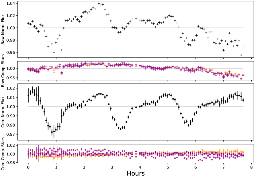
Figure 1: High Cadence, $J$-band photometry of SIMP0136 collected at the CFHT on 14 October 2012. (Top) Raw normalized light curves of SIMP0136. (Second Row) Raw normalized light curves of comparison stars. (Third Row) Corrected light curves for SIMP0136. (Bottom) Corrected light curves for comparison stars. Decreased photometric accuracy can be seen at the beginning and end of the observation period due to increased airmass.

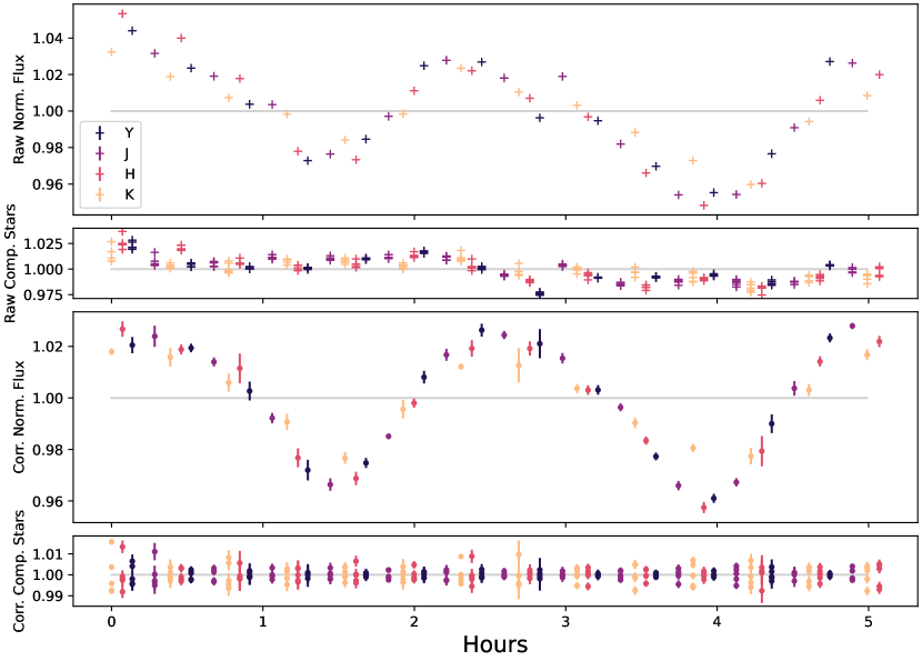
Figure 2: Low Cadence, $Y$/$J$/$H$/$K$ photometry of SIMP0136 collected at the CFHT on 15 October 2012. (Top) Raw normalized light curves of SIMP0136. (Second Row) Raw normalized light curves of comparison stars. (Third Row) Corrected light curves for SIMP0136. (Bottom) Corrected light curves for comparison stars.

3 Methods

To model both planetary-scale atmospheric waves and storms/spots, we modify Imber (Plummer, 2023, 2024), an open source Python code. Imber, the data used in this work, and a tutorial for duplicating our results and figures are openly available via GitHub and Zenodo. Imber was developed and refined in Plummer & Wang (2022, 2023). A more extensive and complete description of the package and its underlying methodology can be found in those articles.

Imber was created to analytically infer surface inhomogeneities (e.g., magnetic spots, storms, and vortices) on stars, brown dwarfs, and directly imaged exoplanets using a Doppler imaging-based technique for spectroscopic data and light curve inversion for photometry. It allows both data types to be included for an integrated multi-modal solution. Imber also includes a numerical simulation module with a full 3D grid to produce forward models of spectra, spectral line profiles, and light curves. Plummer & Wang (2022) demonstrated the numerical and analytical models produce outputs (e.g., line profiles, light curves) with residuals between the two on the order of $0.001$%.

This section details the models we employ as well as the metrics by which we evaluate those models. In §3.1, we describe the wave model we use to fit the photometry. §3.2 provides a brief description of the spotted model we implement via light curve inversion. To infer both wave and spot parameters, we employ Bayesian inference, specifically dynamic nested sampling (Skilling, 2004, 2006; Higson et al., 2019) via Dynesty (Speagle, 2020) within our framework. The inferred models are evaluated based on fit controlled for the number of free parameters (see §3.3).

3.1 Wave Model

For our wave model, we adopt the same approach as Zhou et al. (2022) based on Apai et al. (2017, 2021) and include a bias ($C_{0}$), linear term ($C_{1}$), and the sum of multiple ($N$) sinusoidal functions:

$$F(t)=C_{0}+C_{1}t+\sum_{i}^{N}A_{i}\sin(2\pi t/P_{i}+\theta_{i}).$$ (1)

The linear term ($C_{1}$) accounts for a variation on time scales greater than our observation window. $A_{i}$, $P_{i}$, and $\theta_{i}$ are the $i^{\rm th}$ order amplitude, period, and phase. The free parameters are $C_{0}$, $C_{1}$, $A_{i}$, $P_{i}$, and $\theta_{i}$. Each additional wave adds three additional free parameters; therefore, the expression for the number of free parameters is thus: $m=3N+2$.

Uniform priors are assumed for each free parameter in the wave model. Based on SIMP0136’s photometric variation of ${\sim}5\%$ in each NIR band, the individual wave components amplitudes ($A_{i}$) have a range of $2.5\pm 2.5\%$. For the period, we adjust the range of periods based on the results of the Lomb-Scargle Periodogram in §4.1. Phase varies $180^{\circ}\pm 180^{\circ}$. The bias is allowed to vary by $\pm 0.25$ and the slope by $\pm 0.1\,\rm{h^{-1}}$.

3.2 Storm/Spot Model

Imber was initially designed to both simulate spotted features’ effects on observations and to infer spot parameters given a set of observational data. Here, we will briefly summarize the spotted model, but the authors refer readers to Plummer & Wang (2022, 2023) for a more rigorous explanation.

To enable computationally inexpensive Bayesian inference, the 2D stellar/substellar surface is represented by a 1D flux array. Baseline flux is modeled with a broadening kernel (Gray, 2008) with linear limb darkening coefficients selected based on values derived by fitting Luhman 16B’s spectral line profile (due to similar spectral type and $\rm{T_{eff}}$) in Plummer & Wang (2022). Spots are modeled as Gaussian deviations to the baseline kernel to which bright spots add flux and dark spots subtract flux. The added/subtracted flux is scaled by the spot’s temperature contrast and apparent size. Size is determined based on the spot radius and also latitudinal and longitudinal foreshortening due to the viewing angle (Lambert’s Cosine Law). Object inclination is accounted for with rotation matrices  (Euler-Rodrigues formula, Shuster, 1993). The summed 1D flux at each time step is used to create the modeled light curve.

For this work, Imber was modified to allow both radius and temperature contrast to evolve in value from one rotation to the next. The code currently works by setting the rotation by which the evolution is complete, it then varies the spot parameter (radius or contrast) linearly at each time step over one full rotation, thereby, accounting for dynamic atmospheric activity.

The number of spots drives the number of free parameters for these models. Each spot has a latitude, longitude, radius, and temperature contrast. Similar to the wave models, we also include a bias to account for an unknown mean baseline flux. If spot evolution is incorporated into the model, each evolution increases the number of spot parameters. The model leads to the following expression for the number of free parameters: $m=1+N(4+2E)$, where $N$ is the number of spots and $E$ is the number of spot evolutions.

Similar to the wave model, we assume uniform priors for the spotted model free parameters. Latitude and longitude priors encompass the entire sphere ($\pm 90^{\circ}$ and $\pm 180^{\circ}$ respectively). Radius is sampled from $30\pm 30^{\circ}$. Contrast varies uniformly from +1 (completely dark spot) to -1 (twice the background brightness).

3.3 Model Performance Metrics

To compare the relative merits of each model, we will use goodness-of-fit tests ($\chi^{2}$ and reduced-$\chi^{2}$) and the Bayesian Information Criterion (BIC) to provide metrics. Reduced-$\chi^{2}$ is computed as

$$\chi^{2}_{\nu}=\frac{\chi^{2}}{\nu}=\frac{\chi^{2}}{n-m}=\frac{1}{n-m}\sum_{i=1}^{n}\frac{(O_{i}-M_{i})^{2}}{\sigma^{2}}$$ (2)

where $n$ is the number of data points (observations), $m$ is the number of free parameters, $O_{i}$ and $M_{i}$ are the $i^{\rm th}$ data points for the observation and model respectively, and $\sigma$ is the photometric uncertainty.

We use the following expression to calculate BIC (Kass & Raftery, 1995):

$$\text{BIC}=\chi^{2}+m\ln(n)$$ (3)

For $\chi^{2}$, $\chi^{2}_{\nu}$, and BIC, a smaller value denotes a better fit. BIC and $\chi^{2}_{\nu}$ account for both fit and the number of free parameters, thereby, weighting against more complex models.

4 Results

In this section, we focus on fitting the CFHT data with our wave and spotted models described in §3. Prior to performing these fits, we first perform Lomb-Scargle periodogram analysis (§4.1) on the data to gain a fundamental understanding of the periodic signals. We then use the aforementioned models to fit the 14 October 2012 and 15 October 2012 light curves in §4.2.1 and §4.2.2 respectively.

4.1 Lomb-Scargle Periodogram Analysis

To ascertain the dominant periodic signals within each light curve, we employ the Lomb-Scargle (L-S) Periodogram (Lomb, 1976; Scargle, 1982). As with similar analyses of brown dwarf variability  (e.g., Zhou et al., 2022), we use the LombScargle Python class within astropy (Astropy Collaboration et al., 2013, 2018, 2022) and plot the results in period-space (see Figure 3).

The L-S periodogram returns peak signals at approximately SIMP0136’s rotational period (2.414 h). It should be noted that other studies retrieved similar periods  (e.g., Artigau et al., 2009). The 14 October 2012, high cadence $J$-band photometry demonstrates a prominent peak at $2.412\,\rm{h}$ (corresponding to $k=1$) and at $1.248\,\rm{h}$ ($k=2$). Similarly, the 15 October 2012, low cadence data returns peaks at $2.434\,\rm{h}$, $2.434\,\rm{h}$, $2.457\,\rm{h}$, and $2.504\,\rm{h}$ for the $J$, $H$, and $K$ bands respectively. Longer wavelengths exhibit longer $k=1$ periods. Interestingly, on 15 October 2012, the $Y$ and $J$ bands’ $k=1$ waves have the same periods with small differences in periods for higher wavenumbers.

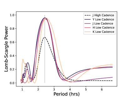
Figure 3: Lomb-Scargle Periodogram. Each NIR band demonstrates a prominent peak at the previously measured rotational period ($\sim 2.4$ h). High cadence, $J$-band data also shows a significant secondary peak at $\sim 1.2$ h, likely indicating a second harmonic. Vertical (gray) line denotes SIMP0136’s previously inferred rotational period, $2.414\pm 0.078$ h (Yang et al., 2016).

4.2 Model Fitting

We fit the SIMP0136 photometry from each observational period and NIR band with both wave (see §3.1) and spotted models (see §3.2) to determine the primary driver of the planetary-mass object’s spectrophotometric variability. Table 1 summarizes the computed $\chi^{2}_{\nu}$, $\chi^{2}$, and BIC values for each model. The preferred model (ranked by $\chi^{2}_{\nu}$) is shown at the top of each category; each alternate model has an associated $\Delta\chi^{2}$ and $\Delta$BIC, denoting its performance with respect to the best fitting model.

4.2.1 High-Cadence Data

We fit the 14 October 2012, high-cadence $J$-band data with both wave and spotted models. For the wave models, we test $N$ = 1 through 3 with improvement seen up to and including 3 waves. We find the 3-wave model is strongly preferred. 4-wave models fail to converge, presumably due to too many free parameters ($m=14$). We test 1 and 2 spot models, both with and without spot evolution. We attempt 3-Spot models but the models do not converge on a solution.

Table 1: Model Comparison: $\chi^{2}$, BIC, observations ($n$), and free parameters ($m$)

Observation Date	NIR Band	Model	$\chi^{2}_{\nu}$	$\chi^{2}$	$\Delta\chi^{2}$	BIC	$\Delta$BIC	$m$
14 October 2012	$J$	3-wave	1.5	149	0	201	0	11
	($n=109$)	2-wave	2.4	247	+97.9	284	+ 83.8	8
		2-spot (evolving)	3.2	302	+154	363	+163	13
		2-spot	3.9	389	+240	431	+230	9
15 October 2012	$Y$	2-wave	1.5	7.7	0	29	0	8
	($n=13$)	1-spot (evolving)	4.4	26.1	+18.4	44.1	+15.9	7
		1-spot	5.7	45.3	+37.6	58.1	+29.9	5
		1-wave	7.3	58.3	+50.6	71.1	+42.9	5
	$J$	2-wave	2.1	10.5	0	31.0	0	8
	($n=13$)	1-spot (evolving)	7.0	41.9	+31.4	59.9	+28.8	7
		1-wave	10.4	82.8	+72.3	95.6	+64.6	5
		1-spot	12.2	97.6	+87.1	110	+79.4	5
	$H$	2-wave	1.8	10.5	0	31.6	0	8
	($n=14$)	1-wave	6.8	61.5	+51.0	74.7	+43.1	5
		1-spot	8.6	77.2	+66.7	90.4	+58.8	5
		1-spot (evolving)	9.1	64.0	+53.5	82.5	+50.9	7
	$K$	2-wave	1.0	5.75	0	26.9	0	8
	($n=14$)	1-wave	2.6	23.5	+17.8	36.7	+9.8	5
		1-spot (evolving)	5.6	39.4	+33.7	57.9	+31.0	7
		1-spot	26.0	234	+228	247	+221	5
	$Y+J+H+K$	2-wave	11.1	509	0	541	0	8
	(n = 54)	2-spot	12.8	576	+67	612	+71.0	9
		1-spot (evolving)	13.7	642	+133	670	+129	7
		1-spot	13.8	675	+166	695	+154	5

Figure 4 shows the preferred 3-wave model with wavenumbers: $k=1$, $2$, and $3$. Wave amplitude decreases with increasing wavenumber. The $k=1$ period ($P_{1}=2.41\pm 0.01$ h) matches the previously measured rotational period  ($2.414\pm 0.078$ h, Yang et al., 2016). The $k=2$ and $k=3$ waves’ periods ($P_{2}=1.21\pm 0.01$ h and $P_{3}=0.80\pm 0.01$ h) are approximately half and one-third SIMP0136’s rotational period. Based on the Nyquist sampling criterion alone, the 14 October 2012, $J$-band mean cadence (0.0715 h) can theoretically detect signals with wavenumbers $\lesssim 16$, so higher order wave components may be missed due to insufficient signal-to-noise (S/N) ratio. Wave components parameters are summarized in Table 2.

We find that SIMP0136 has a $J$-band peak-to-peak variability of $3.85\pm 0.14\%$ for 14 October 2012. Here we compute the % variability based on the minimum and maximum values of the 3-wave model during the observational period. The uncertainty value is computed using the mean of the model standard deviation. The photometric variability measured for 14 October 2012 is lower than that seen the following night, suggesting a dynamic atmosphere over a relatively short time-span.

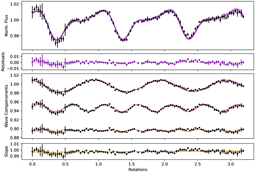
Figure 4: High cadence, 14 October 2012, $J$-band observations and 3-wave model. Shaded regions are $1\sigma$ uncertainty. Rotations are based on a period of 2.414 h (Yang et al., 2016). (Top) The inferred 3-wave model fitted to observations. (Second Row) Residuals. (Third Row) 3-wave components with wave numbers ($k$) $\approx$ 1, 2, and 3 and periods of 2.41  h, 1.21 h, and 0.80 h respectively. To demonstrate each component wave’s fit, the remaining waves and long-term linear terms are subtracted from the data. (Bottom) Linear term with wave components subtracted from the data.

Table 2: Inferred Wave Component Parameters: Amplitude ($A_{i}$), Period ($P_{i}$), and Phase Shifts ($\theta_{i}$))

Observation Date	NIR Band	Wavenumber ($k$)	$A_{i}$ (%)	$P_{i}$ (h)	$\theta_{i}$ (deg)
14 October 2012	$J$	1	$1.29\pm 0.02$	$2.41\pm 0.01$	$112.43\,^{+2.32}_{-2.33}$
		2	$0.81\pm 0.02$	$1.21\pm 0.01$	$17.65\,^{+3.69}_{-3.84}$
		3	$0.21\pm 0.02$	$0.80\pm 0.01$	$239.81\,^{+16.71}_{-16.83}$
15 October 2012	$Y$	1	$2.85\pm 0.11$	$2.42\pm 0.03$	$58.00\,^{+4.85}_{-5.12}$
		2	$0.75\pm 0.11$	$1.27\pm 0.02$	$205.83\,^{+15.54}_{-15.05}$
	$J$	1	$2.94\,^{+0.08}_{-0.07}$	$2.43\pm 0.02$	$57.95\,^{+3.14}_{-3.23}$
		2	$0.67\pm 0.08$	$1.26\pm 0.02$	$190.91\,^{+13.78}_{-12.19}$
	$H$	1	$2.86\pm 0.09$	$2.44\pm 0.03$	$56.93\,^{+4.82}_{-4.94}$
		2	$0.68\,^{+0.11}_{-0.10}$	$1.27\pm 0.02$	$182.53\,^{+15.86}_{-16.58}$
	$K$	1	$1.88\pm 0.09$	$2.43\pm 0.04$	$52.29\,^{+7.19}_{-7.06}$
		2	$0.35\pm 0.10$	$1.27\pm 0.04$	$151.59\,^{+34.29}_{-32.74}$
	$Y+J+H+K$	1	$2.62\pm 0.04$	$2.41\pm 0.01$	$51.95\,^{+2.11}_{-2.10}$
		2	$0.57\pm 0.04$	$1.26\pm 0.01$	$175.41\,^{+8.44}_{-9.30}$

The retrieved 3-wave model contains two features that could allow for multi-rotational light curve evolution: offset phases between components and a long-term linear term (slope). The offset phases allow the superposition of each wave to create a dynamic observed light curve. The Bayesian inference also retrieves a $+0.03\pm 0.01\,\%\cdot\rm{h^{-1}}$ linear slope term, demonstrating a gradual increase in flux and hints at dynamics on timescales longer than the period of observation.

Here we briefly highlight a few features from less preferred models. The 2-wave model (second most preferred) retrieves the same period/wavenumber as the 3-wave model’s highest amplitude waves: $k=1\ \rm{and}\ 2$, adding further support to the 3-wave model. The 2-spot model in which spots were allowed to evolve in size and contrast over each rotation returned both a dark spot (radius ${\sim}20^{\circ}$) and bright spot (radius ${\sim}10^{\circ}$) and was the third most preferred model. The spots were located at opposite polar latitudes (${\sim}\pm 60^{\circ}$) and varied in both size and contrast over each rotation. The spotted model results will be discussed in further detail in §5.1.

4.2.2 Low Cadence Data

The 15 October 2012 observations provide lower cadence data with significantly fewer data points: 13, 13, 14, and 14 for the $Y$, $J$, $H$, and $K$ bands respectively. The mean cadence between observations of 0.385 h corresponds to maximum detectable wavenumbers $\lesssim 3$ based on the Nyquist sampling criterion. Likely due to this result, for each NIR band, we are only able to constrain $k=1\ \rm{and}\ 2$ wave models. 3-wave models do not converge, likely due to the low cadence and small number of observations in each band.

Similar to the high cadence, 15 October 2012 data, multi-wave models outperform spotted models for each individual band and when all four NIR bands are fit simultaneously (see Table 1). The preferred 2-wave models for each NIR band are remarkably similar with each band retrieving $k=1,2$ models with periods at the rotational rate and half the rotational rate (see Table 2 and Figure 5). The phase offsets also appear similar with each component’s $k=1$ wave having a phase between $52^{\circ}-58^{\circ}$ and $k=2$ phases ranging between $152^{\circ}-206^{\circ}$ but with overlapping 1$\sigma$ uncertainties. Matching expectations, the simultaneous, composite $Y+J+H+K$ fit retrieves a 2-wave model which is approximately the average of the individual NIR band solutions.

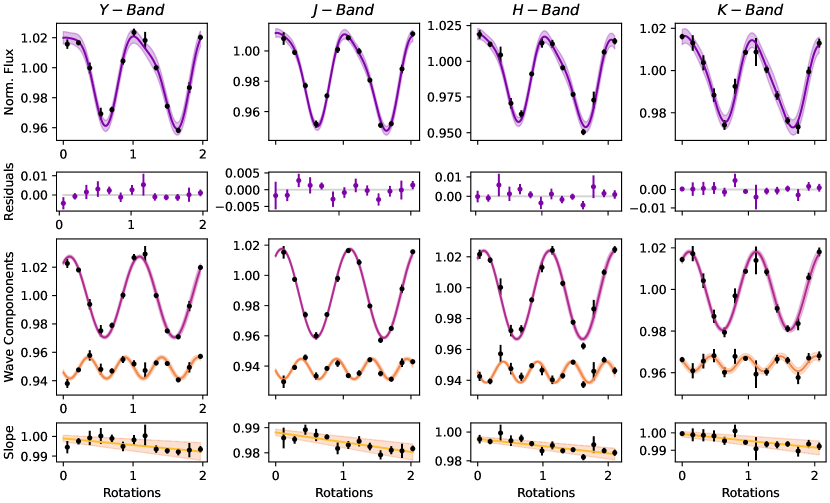
Figure 5: Low cadence, 15 October 2012, $Y$/$J$/$H$/$K$-band observations and 2-wave models. Shaded regions are $1\sigma$ uncertainty. Rotations are based on a period of 2.414 h (Yang et al., 2016). (Top Row) Inferred 2-wave model fitted to observations. (Second Row) Residuals. (Third Row, First Column) $Y$-band, components with wave numbers ($k$) $\approx$ 1 and 2 and periods of 2.42  h and 1.27 h respectively. (Third Row, Second Column) $J$-band, components with wave numbers ($k$) $\approx$ 1 and 2 and periods of 2.43  h and 1.26 h respectively. (Third Row, Third Column) $H$-band, components with wave numbers ($k$) $\approx$ 1 and 2 and periods of 2.44  h and 1.27 h respectively. (Third Row, Fourth Column) $K$-band, components with wave numbers ($k$) $\approx$ 1 and 2 and periods of 2.43  h and 1.27 h respectively. (Bottom Row) Linear term data and fit. Each wave component and linear term is decomposed as described in Figure 4.

Using the 2-wave models, we compute peak-to-peak variability of $6.17\pm 0.46\%$, $6.45\pm 0.33\%$, $6.51\pm 0.42\%$, and $4.33\pm 0.38\%$ for the $Y$, $J$, $H$, and $K$ bands respectively. Both % variability and uncertainty are computed as described in §4.2.1. The high variability ($>5\%$) found here is broadly consistent with previous observations of SIMP0136 (Artigau et al., 2009; Apai et al., 2013; Metchev et al., 2013; Radigan et al., 2014; Wilson et al., 2014; Croll et al., 2016; Apai et al., 2017; McCarthy et al., 2024).

As can be seen in the bottom panel of Figure 5, each NIR band retrieval includes a negative linear slope with values of $-0.14\pm 0.06\,\%\cdot\rm{h^{-1}}$, $-0.16\pm 0.04\,\%\cdot\rm{h^{-1}}$, $-0.21\pm 0.05\,\%\cdot\rm{h^{-1}}$ and $-0.16\pm 0.05\,\%\cdot\rm{h^{-1}}$ for the $Y$, $J$, $H$, and $K$ bands respectively. This is a steeper slope with the opposite sign as that seen in the 14 October 2012 data the night prior. The variation may lend evidence to unmodeled waves or other dynamics with timescales greater than the period of observation.

Spotted models have greater difficulty modelling the low cadence data. Evolving 2-spot models require approximately an equal number of free parameters as there are data points (and are therefore not considered) while non-evolving, 2-spot models have difficulty converging (with the exception of the composite $Y+J+H+K$ fit which has the benefit of a higher number of observations). Both evolving and non-evolving 1-spot models retrieve polar spots (${\sim}70^{\circ}-80^{\circ}$) with radii of ${\sim}30^{\circ}$. Evolving 1-spot models tend to outperform non-evolving models, with the exception being the $H$ band where spot evolution is preferred by BIC but not $\chi^{2}_{\nu}$.

5 Discussion

5.1 Storms or Waves as Primary Variability Driver?

As can be seen in Table 1, wave models outperform spotted models in terms of $\chi^{2}$, $\chi^{2}_{\nu}$, and BIC. Here we seek to explore physical explanations for these results.

To further understand SIMP0136’s atmospheric dynamics, we will use two planetary-scale parameters: the Rossby deformation radius  ($L_{D}$, e.g., Gill, 1982) and the Rhines scale  ($L_{\beta}$, Rhines, 1975). The Rossby deformation radius is the length at which rotational (Coriolis) effects become important (Gill, 1982), and it can also be seen as the typical scale for atmospheric storms and vortices  (e.g., Tan & Showman, 2021b; Zhou et al., 2022). The Rossby deformation radius is computed (in km) as follows (Showman et al., 2013):

$$L_{D}=\frac{U}{2\Omega\sin{\phi}},$$ (4)

where $U$ is the flow speed, $\Omega$ is the angular rotational speed, and $\phi$ is latitude.

At lengths greater than the Rhines scale, atmospheric structures transition from turbulent features to zonal jets as seen on Solar System planets  (e.g., Cho & Polvani, 1996; Showman et al., 2010, 2013; Haqq-Misra et al., 2018); here the Rhines scale is computed (in km):

$$L_{\beta}=\sqrt{\frac{UR}{2\Omega\cos{\phi}}},$$ (5)

where $R$ is the object’s radius

Both inferred spots exceed the Rossby deformation radius and Rhines scale for SIMP0136, meaning the retrieved spotted models are likely unphysical. Considering the spotted model with the best $\chi^{2}_{\nu}$ (see Table 1), the high-cadence $J$-band, 2-spot model with size and contrast evolution, we compute the Rossby deformation radius and Rhines scale at the inferred spot latitude. We conservatively assume a flow velocity ($U$) of $1000\,\rm{m\,s^{-1}}$ based on the brown dwarf 2MASS J10475385+2124234’s (Burgasser et al., 1999) measured wind speed of $650\,\rm{m\,s^{-1}}$ (Allers et al., 2020). We assume a planetary radius of 1.15 $R_{J}$ based on spectral energy distribution analysis of SIMP0136 by Vos et al. (2023). These assumptions result in $L_{D}=0.9^{\circ}$ and $L_{\beta}=11.8^{\circ}$ for latitudes of $\pm 60^{\circ}$. The dark spot at latitude $-62.36^{\circ}\,{}^{+1.37^{\circ}}_{-1.23^{\circ}}$ has inferred radii varying from $23.68^{\circ}\,{}^{+4.67^{\circ}}_{-3.00^{\circ}}$ to $20.27^{\circ}\,{}^{+5.77^{\circ}}_{-3.31^{\circ}}$. The bright spot has a latitude of $+56.77^{\circ}\,{}^{+6.28^{\circ}}_{-19.04^{\circ}}$ and radii ranging from $11.20^{\circ}\,{}^{+3.24^{\circ}}_{-2.33^{\circ}}$ to $10.78^{\circ}\,{}^{+2.73^{\circ}}_{-1.99^{\circ}}$. For each spot, we can see the inferred radii exceed $L_{D}$ and $L_{\beta}$. It is also unlikely that a group of adjacent spots of equivalent summed size are responsible for the observed variability as the same arguments above would require such spots to be in separate latitudinal bands (based on the Rhines scale) in which differential rotation would disperse coherently-structured spot groupings.

The retrieved spots’ polar latitudes also argue against a spotted model explaining SIMP0136’s variability. When exploring different inclinations through GCMs, objects viewed equator-on generate higher variability light curves than those viewed pole-on (Tan & Showman, 2021b). For rotational periods on the scale of SIMP0136 (${\sim}2.5$ h), GCMs also demonstrate that equatorial regions have more enhanced temperature variation and cloud vertical extent than polar latitudes. This is in alignment with observations indicating that brown dwarfs’ equatorial regions are more variable and redder (Vos et al., 2017, 2018, 2020, 2022) and also cloudier (Suárez et al., 2023) than higher latitudes. This argument implies that polar structures similar to Saturn’s polar hexagonal feature (Godfrey, 1988) or Jupiter’s circumpolar cyclones (Bolton et al., 2017; Adriani et al., 2018; Orton et al., 2017) are also unlikely to be the dominant driver of SIMP0136’s variability.

5.2 Planetary-scale Waves in Substellar Atmospheres

The preference for atmospheric waves found in this work is in agreement with prior studies of SIMP0136 photometry (Apai et al., 2017; McCarthy et al., 2024) as well as other L/T transition dwarfs (Apai et al., 2021; Zhou et al., 2022; Fuda et al., 2024). Similar to our results in §4.2.1 and §4.2.2, peak signals corresponding to $k=1$ and $k=2$ waves were identified for SIMP0136 (Apai et al., 2017). Based on observations over 100 rotations, Luhman 16B was found to also contain signals corresponding to $k=1,2$ waves (Apai et al., 2021; Fuda et al., 2024). For VHS 1256 b, a 3-wave model was found to best fit observations over 2 rotations (Zhou et al., 2022). The 3-wave model was comprised of two waves ($P_{1},P_{2}=18.8\pm 0.2\,\rm{h},15.1\pm 0.2\,h$), less than the rotational period  ($22.02\pm{0.04}\,\rm{h}$, Zhou et al., 2020), forming a beating pattern and a third, $k=2$ wave with $P_{3}=10.6\pm 0.1\,\rm{h}$ (Zhou et al., 2022).

Brown dwarf 3D GCMs also support atmospheric waves driving variability at equatorial latitudes. For rapid rotators like SIMP0136, GCMs exhibit equatorial waves with longer zonal wavelengths and lower wavenumber values (similar to those found in §4.2.1 and 4.2.2), as well as the enhanced cloud coverage and temperature variation in their equatorial regions discussed in §5.1 (Tan & Showman, 2021b). Strong evidence is also found for cloud radiative feedback-driven Kelvin waves (and more tentative evidence for Rossby waves) zonally propagating at equatorial latitudes, contributing to light curve variability (Tan & Showman, 2021b). Kelvin waves move along a barrier, which in this case is formed by the equator (along which, the wave moves eastward); essentially, the forces pushing the fluid pole-ward due to a pressure gradient are balanced by Coriolis forces acting towards the equator in eastward moving fluids  (e.g., Gill, 1982). Rossby waves, an additional species of large-scale atmospheric wave, are driven by the conservation of potential vorticity (a fluid mechanics analog to the conservation of angular momentum) and the variation of the Coriolis parameter with latitude (Rossby, 1945).

Planetary-scale waves have been observed to play an important role in the atmospheric dynamics of Jupiter. Quasi-stationary and alternating patterns of relatively cloud-free NIR hot-spots and cooler ammonia cloud-enhanced plumes have long been observed to be associated with the jet at the boundary of Jupiter’s North Equatorial Belt (NEB) and Equatorial Zone (EZ) (Choi et al., 2013). These features are widely considered to be driven by a Rossby wave within Jupiter’s equatorial region (Allison, 1990; Showman & Dowling, 2000; Friedson, 2005) with the wave crests correlating to the ammonia aerosol-enhanced plumes and troughs with cloud-free regions due to condensate sublimation (de Pater et al., 2016; Fletcher et al., 2016, 2020).

5.3 Cloud Modulation and Breakup Associated with Atmospheric Waves

Multi-band photometry offers the opportunity to explore if cloud modulation associated with planetary-scale waves (as seen in brown dwarf GCMs and observations of Jupiter) exists in SIMP0136’s weather layer. If the variability from the waves is associated with silicate and metal clouds (Suárez & Metchev, 2022; Vos et al., 2023; McCarthy et al., 2024), the light curve minima are where we would expect cloud coverage. In this scenario, the light curve maxima would be associated with hot spots, atmospheric areas of depleted aerosols in which light from deeper atmospheric layers is observable. We expect clouds to scatter and therefore redden light, and indeed, cloudier brown dwarfs have been found to be redder than less cloudy objects (Suárez & Metchev, 2022). Light curve minima should be redder and maxima bluer if this hypothesis is true. A lack of correlation between the light curves and NIR color might support an alternate theory such as convective fingering (Tremblin et al., 2016, 2019).

Using the $Y$/$J$/$H$/$K$, 15 October 2012 photometry, we conduct a preliminary analysis to determine if the light curve minima are associated with redder NIR colors and if light curve maxima are associated with corresponding bluer colors. As a proxy for color, we use the normalized flux of the 2-wave models to create $Y-J$, $J-H$, and $H-K$ color time series (see Figure 6). Qualitatively it can be seen that for each color series, the light curve (here we use the simultaneously-inferred composite $Y+J+H+K$ curve) minima approximately correspond to significant dips towards redder colors while maxima correspond to bluer colors. This behaviour is more pronounced for longer wavelengths (e.g., $H-K$). The $H-K$ color time series leads the composite $Y+J+H+K$ curve to a small degree while $Y-J$ and $J-H$ each lag the light curve minima. We interpret these results as tentative evidence for complex vertical cloud structure with (presumably silicates and metal) clouds located at the minima and cloud-free regions existing at the maxima due to condensate sublimation.

Follow-up observations using, ideally space-based, platforms with NIR and mid-IR (MIR) spectroscopic capabilities such as the James Webb Space Telescope (JWST) would have the capability to gather broad wavelength times series (see e.g., JWST Cycle 2 GO Program 3548, PI J. Vos). With this data, broadband flux variations could be compared to variations in cloud coverage and chemical abundances, further constraining the nature of planetary-scale waves.

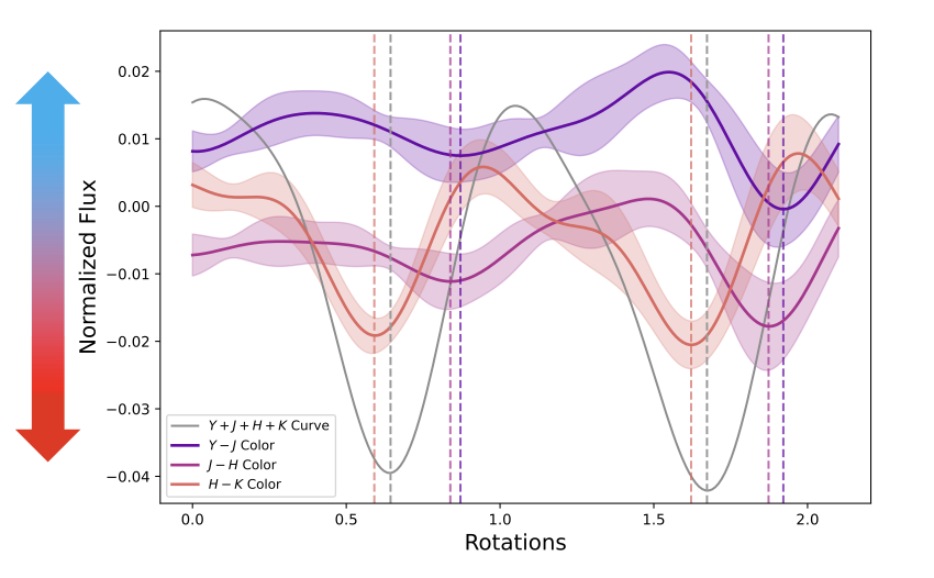
Figure 6: Color time series comparison to composite $Y+J+H+K$ light curve (gray). Shaded regions are $1\sigma$ uncertainty. Vertical dashed lines denote color series and light curve minima. Qualitatively, it can be seen that composite light curve minima correspond to reddening (i.e. low flux in $Y-J$, $J-H$, and $H-K$ corresponds to redder color indices). This provides evidence for cloud scattering (see §5.3). Light curve maxima correspond to bluer, presumably relatively cloud-free regions. The $Y-J$ and $J-H$ color series are approximately in phase but the $H-K$ solution is ${\sim}90^{\circ}$ out of phase with the remaining color series, offering evidence of SIMP0136’s complex vertical cloud structure.

5.4 Phase Shifts Between NIR Bands

As wavelengths are sensitive to different pressure levels in brown dwarf and planetary-mass object atmospheres  (e.g., Figure 4 in McCarthy et al., 2024), phase shifts between NIR bands can indicate inhomogeneity in their vertical structures. Large phase shifts (${\sim}90{\textendash}180^{\circ}$) have been detected between shorter NIR bands (e.g., $J$ and $K$) and longer wavelengths (e.g., Spitzer/Infrared Array Camera Ch.1 [$3.6\,\mu m$] and Ch.2 [$4.5\,\mu m$]) (Buenzli et al., 2012; Yang et al., 2016) for 2MASS J22282889–4310262  (T6.5, Burgasser et al., 2003), 2MASS J15074769–1627386  (L5, Reid et al., 2000), and 2MASS J18212815+1414010  (L5, Looper et al., 2008).

L/T transition objects such as VHS 1256 b, Luhman 16B (T0.5), 2MASS J21392676+0220226  (2M2139, T1.5, Reid et al., 2008), and SIMP0136 have demonstrated, in general, subtler phase shifts than earlier L and later T dwarfs. Zhou et al. (2022) collected 42 h of time series observation of VHS 1256 b using the Hubble Space Telescope (HST)/Wide Field Camera 3 (WFC3) and identified no discernible phase shift between the F127M ($1.270\pm 0.035\,\rm{\mu m}$), F139M ($1.385\pm 0.035\,\rm{\mu m}$), and F153M ($1.530\pm 0.035\,\rm{\mu m}$) filters. Observing Luhman 16B in optical and NIR bands, Biller et al. (2013) detected significant phase offsets, but Buenzli et al. (2015) found the $J$, $H$, and water bands to all be in phase. Apai et al. (2013) did not find phase shifts in either 2M2139 or SIMP0136 using HST/WFC3 G141 data, but Yang et al. (2016) found modest phase shifts (${\sim}30^{\circ}$) between light curves derived from HST/WFC3 G141 and Spitzer Ch.1 and Ch.2. McCarthy et al. (2024) similarly found phase shifts between $J$ and $K_{s}$ bands of $39.9^{\circ}\,{}^{+3.6^{\circ}}_{-1.1^{\circ}}$ using data collected at the Perkins Telescope Observatory.

Considering the color time series in Figure 6, it can be qualitatively seen that the $H-K$ series is offset by ${\sim}90^{\circ}$ from the $J-H$ and $Y-J$ color series, which are approximately in phase with one another. Adopting a similar approach as McCarthy et al. (2024), we use the signal function within Scipy (Virtanen et al., 2020) to determine the phase shift via cross-correlation. Performing cross-correlation on 5,000 samples from the $H-K$ and $J-H$ solutions provides a phase shift of $93.8^{\circ}\pm 7.4^{\circ}$. This $12.7\sigma$ detection provides evidence for complex vertical cloud structure between the pressure levels corresponding to these NIR bands.

Statistically significant phase shifts between the inferred NIR band wave components are not detected for SIMP0136 in this work (see Table 2). Within each band, the $k=1$ and $k=2$ components are offset by approximately $100^{\circ}-140^{\circ}$ from one another. The $k=1$ components each have phases ranging from $\sim 52^{\circ}-58^{\circ}$. The $k=2$ components have phases ranging from $\sim 150^{\circ}$ to $205^{\circ}$. For both $k=1$ and $k=2$ waves, the phase shifts between NIR bands are less than the $3\sigma$ uncertainty.

Higher cadence observations in both the NIR and MIR, such as those capable by the JWST, would be able to reduce phase uncertainty and detect phase shifts at lower pressure levels (higher altitudes). Such detections would provide further collaborating evidence of cloud modulation associated with planetary-scale waves along with a more complete picture of SIMP0136’s vertical architecture.

6 Summary

To determine the driving source of spectrophotometric variability in SIMP0136, an L/T transition object, we analyze NIR photometry collected at the CFHT on the nights of 14 October 2012 and 15 October 2012. The data provides coverage for ${\gtrsim}5$ rotations of SIMP0136. We modify the publicly available, open source Python code Imber (Plummer, 2023, 2024), developed and honed in Plummer & Wang (2022, 2023), to fit the observed light curves with waves as well as spotted models. Here are our findings:

1. The 14 October 2012, high cadence $J$-band observations are best fit with a 3-wave model consisting of $k=1,2,\ \rm{and}\ 3$ components with periods 2.41 h, 1.21 h, and 0.80 h (see §4.2.1). A linear term with a positive slope is also retrieved and indicates an increase in flux over the period of observation.

2. The 15 October, low cadence $Y$/$J$/$H$/$K$ light curves are each fit with 2-wave models with $k=1\ \rm{and}\ 2$ components (see §4.2.2). Each of these components has periods approximating the rotational period and half the rotational period. In each of the inferred models, the linear term has a negative slope, demonstrating a change from the prior night’s observations.

3. For the spotted models, the retrieved spot radii exceed the Rossby deformation radius and Rhines scale for the inferred latitudes (and assumed mean flow and planetary radius), indicating such spots to likely be unphysical (see §5.1).

4. For the multi-band ($Y$/$J$/$H$/$K$) photometry, the inferred 2-wave models demonstrate correlation with shifts in color (see §5.2). The light curve minima appear to correspond to redder colors while the maxima correspond to bluer flux. This correlation is strongest for the $H-K$ color time series. We propose this may be tentative evidence for planetary-scale waves traveling in the vertical plane of SIMP0136’s atmosphere with enhanced silicate or iron cloud coverage in the wave crests and depleted aerosols in the troughs.

5. We detect a $93.8^{\circ}\pm 7.4^{\circ}$ ($12.7\sigma$) phase offset between the $H-K$ and $J-H$ color series, providing evidence for complex vertical cloud structure in SIMP0136’s atmosphere.

Moving forward, a greater understanding of the true nature of planetary-scale waves potentially driving brown dwarf and planetary-mass object variability can be achieved by multi-rotational and quasi-simultaneous observations in the NIR and MIR by platforms such as JWST. Spectroscopic modes would help to discern if the reddening associated with NIR light curve minima is tied to variations in cloud coverage or chemical abundances. Both photometric and spectroscopic modes could further constrain phase shifts between NIR and MIR bands and color indices, providing a greater understanding of SIMP0136’s vertical structure throughout its atmospheric layers.

References

- Ackerman & Marley (2001) Ackerman, A. S., & Marley, M. S. 2001, ApJ, 556, 872, doi: 10.1086/321540
- Adriani et al. (2018) Adriani, A., Mura, A., Orton, G., et al. 2018, Nature, 555, 216, doi: 10.1038/nature25491
- Allers et al. (2020) Allers, K. N., Vos, J. M., Biller, B. A., & Williams, P. K. G. 2020, Science, 368, 169, doi: 10.1126/science.aaz2856
- Allison (1990) Allison, M. 1990, Icarus, 83, 282, doi: 10.1016/0019-1035(90)90069-L
- Apai et al. (2021) Apai, D., Nardiello, D., & Bedin, L. R. 2021, ApJ, 906, 64, doi: 10.3847/1538-4357/abcb97
- Apai et al. (2013) Apai, D., Radigan, J., Buenzli, E., et al. 2013, ApJ, 768, 121, doi: 10.1088/0004-637X/768/2/121
- Apai et al. (2017) Apai, D., Karalidi, T., Marley, M. S., et al. 2017, Science, 357, 683, doi: 10.1126/science.aam9848
- Artigau et al. (2009) Artigau, É., Bouchard, S., Doyon, R., & Lafrenière, D. 2009, ApJ, 701, 1534, doi: 10.1088/0004-637X/701/2/1534
- Artigau et al. (2006) Artigau, É., Doyon, R., Lafrenière, D., et al. 2006, ApJ, 651, L57, doi: 10.1086/509146
- Astropy Collaboration et al. (2013) Astropy Collaboration, Robitaille, T. P., Tollerud, E. J., et al. 2013, A&A, 558, A33, doi: 10.1051/0004-6361/201322068
- Astropy Collaboration et al. (2018) Astropy Collaboration, Price-Whelan, A. M., Sipőcz, B. M., et al. 2018, AJ, 156, 123, doi: 10.3847/1538-3881/aabc4f
- Astropy Collaboration et al. (2022) Astropy Collaboration, Price-Whelan, A. M., Lim, P. L., et al. 2022, ApJ, 935, 167, doi: 10.3847/1538-4357/ac7c74
- Biller et al. (2013) Biller, B. A., Crossfield, I. J. M., Mancini, L., et al. 2013, ApJ, 778, L10, doi: 10.1088/2041-8205/778/1/L10
- Bolton et al. (2017) Bolton, S. J., Adriani, A., Adumitroaie, V., et al. 2017, Science, 356, 821, doi: 10.1126/science.aal2108
- Buenzli et al. (2015) Buenzli, E., Saumon, D., Marley, M. S., et al. 2015, ApJ, 798, 127, doi: 10.1088/0004-637X/798/2/127
- Buenzli et al. (2012) Buenzli, E., Apai, D., Morley, C. V., et al. 2012, ApJ, 760, L31, doi: 10.1088/2041-8205/760/2/L31
- Burgasser et al. (2002) Burgasser, A. J., Marley, M. S., Ackerman, A. S., et al. 2002, ApJ, 571, L151, doi: 10.1086/341343
- Burgasser et al. (2003) Burgasser, A. J., McElwain, M. W., & Kirkpatrick, J. D. 2003, AJ, 126, 2487, doi: 10.1086/378608
- Burgasser et al. (1999) Burgasser, A. J., Kirkpatrick, J. D., Brown, M. E., et al. 1999, ApJ, 522, L65, doi: 10.1086/312221
- Burrows et al. (2001) Burrows, A., Hubbard, W. B., Lunine, J. I., & Liebert, J. 2001, Reviews of Modern Physics, 73, 719, doi: 10.1103/RevModPhys.73.719
- Burrows & Sharp (1999) Burrows, A., & Sharp, C. M. 1999, ApJ, 512, 843, doi: 10.1086/306811
- Burrows et al. (2006) Burrows, A., Sudarsky, D., & Hubeny, I. 2006, ApJ, 640, 1063, doi: 10.1086/500293
- Cho & Polvani (1996) Cho, J. Y. K., & Polvani, L. M. 1996, Science, 273, 335, doi: 10.1126/science.273.5273.335
- Choi et al. (2013) Choi, D. S., Showman, A. P., Vasavada, A. R., & Simon-Miller, A. A. 2013, Icarus, 223, 832, doi: 10.1016/j.icarus.2013.02.001
- Croll et al. (2016) Croll, B., Muirhead, P. S., Lichtman, J., et al. 2016, arXiv e-prints, arXiv:1609.03587. https://arxiv.org/abs/1609.03587
- Crossfield et al. (2014) Crossfield, I. J. M., Biller, B., Schlieder, J. E., et al. 2014, Nature, 505, 654, doi: 10.1038/nature12955
- Cushing & Roellig (2006) Cushing, M. C., & Roellig, T. L. 2006, in Astronomical Society of the Pacific Conference Series, Vol. 357, The Spitzer Space Telescope: New Views of the Cosmos, ed. L. Armus & W. T. Reach, 66
- de Pater et al. (2016) de Pater, I., Sault, R. J., Butler, B., DeBoer, D., & Wong, M. H. 2016, Science, 352, 1198, doi: 10.1126/science.aaf2210
- Eriksson et al. (2019) Eriksson, S. C., Janson, M., & Calissendorff, P. 2019, A&A, 629, A145, doi: 10.1051/0004-6361/201935671
- Fletcher et al. (2016) Fletcher, L. N., Greathouse, T. K., Orton, G. S., et al. 2016, Icarus, 278, 128, doi: 10.1016/j.icarus.2016.06.008
- Fletcher et al. (2020) Fletcher, L. N., Orton, G. S., Greathouse, T. K., et al. 2020, Journal of Geophysical Research (Planets), 125, e06399, doi: 10.1029/2020JE006399
- Friedson (2005) Friedson, A. J. 2005, Icarus, 177, 1, doi: 10.1016/j.icarus.2005.03.004
- Fuda et al. (2024) Fuda, N., Apai, D., Nardiello, D., et al. 2024, arXiv e-prints, arXiv:2403.02260. https://arxiv.org/abs/2403.02260
- Gagné et al. (2017) Gagné, J., Faherty, J. K., Burgasser, A. J., et al. 2017, ApJ, 841, L1, doi: 10.3847/2041-8213/aa70e2
- Gauza et al. (2015) Gauza, B., Béjar, V. J. S., Pérez-Garrido, A., et al. 2015, ApJ, 804, 96, doi: 10.1088/0004-637X/804/2/96
- Gill (1982) Gill, A. E. 1982, Atmosphere-Ocean Dynamics (Academic Press, Orlando), 662
- Godfrey (1988) Godfrey, D. A. 1988, Icarus, 76, 335, doi: 10.1016/0019-1035(88)90075-9
- Gray (2008) Gray, D. F. 2008
- Haqq-Misra et al. (2018) Haqq-Misra, J., Wolf, E. T., Joshi, M., Zhang, X., & Kopparapu, R. K. 2018, ApJ, 852, 67, doi: 10.3847/1538-4357/aa9f1f
- Higson et al. (2019) Higson, E., Handley, W., Hobson, M., & Lasenby, A. 2019, Statistics and Computing, 29, 891, doi: 10.1007/s11222-018-9844-0
- Hunter (2007) Hunter, J. D. 2007, Computing in Science & Engineering, 9, 90, doi: 10.1109/MCSE.2007.55
- Kass & Raftery (1995) Kass, R. E., & Raftery, A. E. 1995, Journal of the American Statistical Association, 90, 773, doi: 10.1080/01621459.1995.10476572
- Kirkpatrick (2005) Kirkpatrick, J. D. 2005, ARA&A, 43, 195, doi: 10.1146/annurev.astro.42.053102.134017
- Knapp et al. (2004) Knapp, G. R., Leggett, S. K., Fan, X., et al. 2004, AJ, 127, 3553, doi: 10.1086/420707
- Liu et al. (2024) Liu, P., Biller, B. A., Vos, J. M., et al. 2024, MNRAS, 527, 6624, doi: 10.1093/mnras/stad3502
- Lomb (1976) Lomb, N. R. 1976, Ap&SS, 39, 447, doi: 10.1007/BF00648343
- Looper et al. (2008) Looper, D. L., Kirkpatrick, J. D., Cutri, R. M., et al. 2008, ApJ, 686, 528, doi: 10.1086/591025
- Luhman (2013) Luhman, K. L. 2013, ApJ, 767, L1, doi: 10.1088/2041-8205/767/1/L1
- McCarthy et al. (2024) McCarthy, A. M., Muirhead, P. S., Tamburo, P., et al. 2024, arXiv e-prints, arXiv:2402.15001. https://arxiv.org/abs/2402.15001
- McKinney et al. (2010) McKinney, W., et al. 2010, in Proceedings of the 9th Python in Science Conference, Vol. 445, Austin, TX, 51–56
- Metchev et al. (2013) Metchev, S., Apai, D., Radigan, J., et al. 2013, Astronomische Nachrichten, 334, 40, doi: 10.1002/asna.201211776
- Millar-Blanchaer et al. (2020) Millar-Blanchaer, M. A., Girard, J. H., Karalidi, T., et al. 2020, ApJ, 894, 42, doi: 10.3847/1538-4357/ab6ef2
- Orton et al. (2017) Orton, G. S., Hansen, C., Caplinger, M., et al. 2017, Geophys. Res. Lett., 44, 4599, doi: 10.1002/2016GL072443
- Plummer (2024) Plummer, M. 2024, Imber 3.0: Modeling Spectrophotometric Variability of a Planetary-Mass Object, 3.0, Zenodo, doi: 10.5281/zenodo.10729262
- Plummer (2023) Plummer, M. K. 2023, Imber: Doppler imaging tool for modeling stellar and substellar surfaces, Astrophysics Source Code Library, record ascl:2307.033. http://ascl.net/2307.033
- Plummer & Wang (2022) Plummer, M. K., & Wang, J. 2022, ApJ, 933, 163, doi: 10.3847/1538-4357/ac75b9
- Plummer & Wang (2023) —. 2023, ApJ, 951, 101, doi: 10.3847/1538-4357/accd5d
- Puget et al. (2004) Puget, P., Stadler, E., Doyon, R., et al. 2004, in Society of Photo-Optical Instrumentation Engineers (SPIE) Conference Series, Vol. 5492, Ground-based Instrumentation for Astronomy, ed. A. F. M. Moorwood & M. Iye, 978–987, doi: 10.1117/12.551097
- Radigan (2014) Radigan, J. 2014, ApJ, 797, 120, doi: 10.1088/0004-637X/797/2/120
- Radigan et al. (2014) Radigan, J., Lafrenière, D., Jayawardhana, R., & Artigau, E. 2014, ApJ, 793, 75, doi: 10.1088/0004-637X/793/2/75
- Reid et al. (2008) Reid, I. N., Cruz, K. L., Kirkpatrick, J. D., et al. 2008, AJ, 136, 1290, doi: 10.1088/0004-6256/136/3/1290
- Reid et al. (2000) Reid, I. N., Kirkpatrick, J. D., Gizis, J. E., et al. 2000, AJ, 119, 369, doi: 10.1086/301177
- Reiners & Basri (2008) Reiners, A., & Basri, G. 2008, ApJ, 684, 1390, doi: 10.1086/590073
- Rhines (1975) Rhines, P. B. 1975, Journal of Fluid Mechanics, 69, 417, doi: 10.1017/S0022112075001504
- Rossby (1945) Rossby, C. G. 1945, Journal of the Atmospheric Sciences, 2, 187, doi: 10.1175/1520-0469(1945)002<0187:OTPOFA>2.0.CO;2
- Scargle (1982) Scargle, J. D. 1982, ApJ, 263, 835, doi: 10.1086/160554
- Showman et al. (2010) Showman, A. P., Cho, J. Y. K., & Menou, K. 2010, in Exoplanets, ed. S. Seager, 471–516
- Showman & Dowling (2000) Showman, A. P., & Dowling, T. E. 2000, Science, 289, 1737, doi: 10.1126/science.289.5485.1737
- Showman et al. (2013) Showman, A. P., Fortney, J. J., Lewis, N. K., & Shabram, M. 2013, ApJ, 762, 24, doi: 10.1088/0004-637X/762/1/24
- Showman & Kaspi (2013) Showman, A. P., & Kaspi, Y. 2013, ApJ, 776, 85, doi: 10.1088/0004-637X/776/2/85
- Showman et al. (2019) Showman, A. P., Tan, X., & Zhang, X. 2019, ApJ, 883, 4, doi: 10.3847/1538-4357/ab384a
- Shuster (1993) Shuster, M. D. 1993, IEEE Transactions on Aerospace Electronic Systems, 29, 263, doi: 10.1109/7.249140
- Skilling (2004) Skilling, J. 2004, in American Institute of Physics Conference Series, Vol. 735, Bayesian Inference and Maximum Entropy Methods in Science and Engineering: 24th International Workshop on Bayesian Inference and Maximum Entropy Methods in Science and Engineering, ed. R. Fischer, R. Preuss, & U. V. Toussaint, 395–405, doi: 10.1063/1.1835238
- Skilling (2006) Skilling, J. 2006, Bayesian Analysis, 1, 833, doi: 10.1214/06-BA127
- Speagle (2020) Speagle, J. S. 2020, MNRAS, 493, 3132, doi: 10.1093/mnras/staa278
- Suárez & Metchev (2022) Suárez, G., & Metchev, S. 2022, MNRAS, 513, 5701, doi: 10.1093/mnras/stac1205
- Suárez et al. (2023) Suárez, G., Vos, J. M., Metchev, S., Faherty, J. K., & Cruz, K. 2023, ApJ, 954, L6, doi: 10.3847/2041-8213/acec4b
- Tan (2022) Tan, X. 2022, MNRAS, doi: 10.1093/mnras/stac344
- Tan & Showman (2021a) Tan, X., & Showman, A. P. 2021a, MNRAS, 502, 678, doi: 10.1093/mnras/stab060
- Tan & Showman (2021b) —. 2021b, MNRAS, 502, 2198, doi: 10.1093/mnras/stab097
- Thanjavur et al. (2011) Thanjavur, K., Teeple, D., & Yan, C.-H. 2011, in Telescopes from Afar, ed. S. Gajadhar, J. Walawender, R. Genet, C. Veillet, A. Adamson, J. Martinez, J. Melnik, T. Jenness, & N. Manset, 72
- Tremblin et al. (2016) Tremblin, P., Amundsen, D. S., Chabrier, G., et al. 2016, ApJ, 817, L19, doi: 10.3847/2041-8205/817/2/L19
- Tremblin et al. (2019) Tremblin, P., Padioleau, T., Phillips, M. W., et al. 2019, ApJ, 876, 144, doi: 10.3847/1538-4357/ab05db
- Tsuji & Nakajima (2003) Tsuji, T., & Nakajima, T. 2003, ApJ, 585, L151, doi: 10.1086/374388
- Tsuji et al. (1996) Tsuji, T., Ohnaka, K., Aoki, W., & Nakajima, T. 1996, A&A, 308, L29
- Virtanen et al. (2020) Virtanen, P., Gommers, R., Oliphant, T. E., et al. 2020, Nature Methods, 17, 261, doi: 10.1038/s41592-019-0686-2
- Vos et al. (2017) Vos, J. M., Allers, K. N., & Biller, B. A. 2017, ApJ, 842, 78, doi: 10.3847/1538-4357/aa73cf
- Vos et al. (2018) Vos, J. M., Allers, K. N., Biller, B. A., et al. 2018, MNRAS, 474, 1041, doi: 10.1093/mnras/stx2752
- Vos et al. (2022) Vos, J. M., Faherty, J. K., Gagné, J., et al. 2022, ApJ, 924, 68, doi: 10.3847/1538-4357/ac4502
- Vos et al. (2020) Vos, J. M., Biller, B. A., Allers, K. N., et al. 2020, AJ, 160, 38, doi: 10.3847/1538-3881/ab9642
- Vos et al. (2023) Vos, J. M., Burningham, B., Faherty, J. K., et al. 2023, ApJ, 944, 138, doi: 10.3847/1538-4357/acab58
- Wilson et al. (2014) Wilson, P. A., Rajan, A., & Patience, J. 2014, A&A, 566, A111, doi: 10.1051/0004-6361/201322995
- Yang et al. (2016) Yang, H., Apai, D., Marley, M. S., et al. 2016, ApJ, 826, 8, doi: 10.3847/0004-637X/826/1/8
- Zhang & Showman (2014) Zhang, X., & Showman, A. P. 2014, ApJ, 788, L6, doi: 10.1088/2041-8205/788/1/L6
- Zhou et al. (2022) Zhou, Y., Bowler, B. P., Apai, D., et al. 2022, arXiv e-prints, arXiv:2210.02464. https://arxiv.org/abs/2210.02464
- Zhou et al. (2020) Zhou, Y., Bowler, B. P., Morley, C. V., et al. 2020, AJ, 160, 77, doi: 10.3847/1538-3881/ab9e04