Stochastic Gravitational Wave Background from Highly-Eccentric Stellar-Mass Binaries in the Milli-hertz Band
Abstract
Many gravitational wave (GW) sources are expected to have non-negligible eccentricity in the millihertz band. These highly eccentric compact object binaries may commonly serve as a progenitor stage of GW mergers, particularly in dynamical channels where environmental perturbations bring a binary with large initial orbital separation into a close pericenter passage, leading to efficient GW emission and a final merger. This work examines the stochastic GW background from highly eccentric (), stellar-mass sources in the mHz band. Our findings suggest that these binaries can contribute a substantial GW power spectrum, potentially exceeding the LISA instrumental noise at mHz. This stochastic background is likely to be dominated by eccentric sources within the Milky Way, thus introducing anisotropy and time dependence in LISA’s detection. However, given efficient search strategies to identify GW transients from highly eccentric binaries, the unresolvable noise level can be substantially lower, approaching orders of magnitude below the LISA noise curve. Therefore, we highlight the importance of characterizing stellar-mass GW sources with extreme eccentricity, especially their transient GW signals in the millihertz band.
I Introduction
The study of GW signals from eccentric compact object binaries plays an important role in GW astronomy. For example, extensive efforts have been made to measure the residual eccentricity of GW mergers in the data analysis of LIGO, Virgo, KARAGA (LVK) collaboration, which could shed light on the formation mechanisms of compact binaries [1, 2, 3, 4, 5, 6, 7, 8, 9, 10, 11]. However, so far, no confident evidence of residual eccentricity has been detected [see, e.g., 12, 13, 14, 15, 16], primarily because GW radiation tends to circularize the orbit, rendering eccentricity negligible within the LVK frequency band [17, 18]. In the future, the Laser Interferometer Space Antenna (LISA) [19] is expected to observe sources in a lower frequency band (). Consequently, numerous eccentric GW sources, potentially in their earlier evolutionary stages, may be present in the LISA data stream, providing valuable insights into their surrounding environments [see, e.g., 20, 21, 22, 23, 24, 25, 26, 27, 28, 29, 30].
Many eccentric GW sources formed through dynamical channels undergo a progenitor stage before the final merger. In this phase, the compact object binary, initially characterized by a large semi-major axis (e.g., ), attains extreme eccentricity (e.g., ) due to environmental perturbations. Although these sources have an orbital frequency well below the millihertz band, the binary’s pericenter distance, , can become sufficiently close to induce strong millihertz GW emission [see, e.g., 31, 32, 33]. This process leads to orbital energy loss, causing the orbit to shrink and circularize, resulting in a GW merger.
The GW signal emitted by wide, highly eccentric compact binaries exhibits distinctive characteristics compared to quasi-circular ones. In particular, when the binary’s eccentricity is small, the GW signal can be effectively approximated by a near-monochromatic, sinusoidal wave, where the dominant GW frequency is twice the orbital frequency [see, e.g., 34]. However, with an increase in the source’s eccentricity, the GW emission becomes stronger upon each pericenter passage, turning the signal into a burst-like waveform [e.g., see Fig.1 in reference 33]. For example, a compact object binary with eccentricity will emit more than of its GW energy in less than of the orbital period during the pericenter passage, regardless of its components’ masses , and semi-major axis [33].
Various dynamic environments can give rise to stellar-mass bursting GW sources. For example, in dense star clusters, compact object binaries may attain non-negligible eccentricity due to external perturbations like GW capture, binary-single, and binary-binary scattering [e.g., 35, 36, 37, 38, 39, 4, 40, 41, 42, 43, 44, 45, 46, 47]. Highly eccentric mergers can also arise in stellar disks or active galactic nucleus accretion disks [48, 16, 49, 50]. Additionally, fly-by interactions and galactic tides may excite the eccentricity of wide compact object binaries in the galactic field [e.g., 51, 52, 53], potentially leading to observable mergers. Moreover, in a hierarchical triple system (a tight binary orbiting a third body on a much wider ”outer orbit”), the inner binary can undergo eccentricity oscillations via the eccentric Kozai-Lidov (EKL) mechanism [54, 55, 56], becoming a GW source with high eccentricity in the LISA band. These channels can significantly contribute to the overall merger rate of stellar-mass compact objects [e.g., 57, 58, 59, 60, 41, 61, 62, 63, 9].
In this paper, our focus is on the stochastic GW background (GWB) originating from these bursting sources. In particular, as a collective GW signal of unresolved sources, the astrophysical stochastic GWB will compete with other expected LISA science sources, potentially producing a confusion noise that affects LISA sensitivity. Previous efforts have aimed to characterize various stochastic backgrounds, such as the collective GW signal from the galactic population of double white dwarf (DWD) binaries [see, e.g., 64, 65, 66, 67], extragalactic sources [20, Bonetti+2020Enoki2007, 68, 69, 70], and cosmological stochastic backgrounds [71, 72, 73, 74, 40, 75]. Additionally, it was recently suggested that extreme mass ratio inspirals (EMRIs) might have orders of magnitude higher formation rate [76] that may yield an order of magnitude noise level above LISA’s sensitivity level [77]. By understanding these backgrounds, we not only address the potential impact of confusion noise on the parameter estimation of other resolved sources but also extract information about the stochastic background itself, thus constraining the population of GW sources [see, e.g., 78, 77].
As a natural consequence of dynamical formation, the highly eccentric, stellar-mass binaries may create a significant GW background in the LISA band. For example, in our previous studies [33], we anticipate the presence of approximately 3 to 45 detectable bursting binary black holes (BBHs) within the Milky Way, each with a signal-to-noise ratio (SNR) exceeding 5 for the upcoming LISA mission [33]. Beyond these detectable cases, there could be a considerably larger number of bursting sources with SNR values falling below the detection threshold, yet their collective contribution remains significant.
Furthermore, the transient nature of these sources poses challenges in extracting their signals from the detector’s output [79, 31, 32], which potentially leads to a higher noise background level. In particular, the burst detection methods for stellar-mass binaries, especially when multiple sources’ bursts are present in the data stream simultaneously, remain relatively underdeveloped. Thus, there is uncertainty regarding our ability to identify all bursting sources in the detector’s output, even if the sources’ SNR is above the detection threshold. Moreover, the astrophysical burst signals may be intertwined with instrumental noise, such as glitches [see, e.g., 80, 81, 82], and contribute to the unresolved GW background.
We note that, there have been previous works examining the GWB from circular stellar-mass BBHs [see, e.g., 73, 74, 83] and eccentric stellar-mass BBHs at a cosmological distance [see, e.g., 84, 40, 85]. These studies suggested that stellar-mass BBHs can make a non-negligible contribution to future observations, with eccentricity potentially affecting the overall shape of the millihertz GW background. In this work, however, we extend this analysis beyond the cosmological population of BBHs to explore the GWB contribution of highly eccentric sources at close distances, specifically bursting sources in the Milky Way and nearby galaxies. As discussed before, even considering only the Milky Way population, the number of these sources may be substantial [33], and their close distance can potentially yield a significant overall GWB level. Furthermore, the transient nature of their GW emission can affect the pattern of the GWB, with a single bursting source capable of emitting GWs in a wide range of frequencies, which may cause confusion in future observations. In our analysis, we consider the realistic spatial distribution and non-equilibrium formation history of highly eccentric sources.
We organize this paper as follows. In Section II.1, we first demonstrate the properties of bursting GW sources, then discuss their detectability (Section II.2.1) and GW background calculation (Section II.2.2). In Section III, we introduce the population model of bursting sources, then carry out numerical simulations to predict the GW background level from highly-eccentric, stellar-mass BBHs in the Universe (Section III.2). We show the results separately, for the globular clusters (Section III.2.1), galactic field (Section III.2.2), and the galactic nucleus (Section III.2.3). In Section IV, we summarize and discuss the overall effect of stochastic GW background from stellar-mass bursting sources.
Unless otherwise specified, we set .
II Theoretical consideration
II.1 The Properties of GW Bursts from Highly Eccentric Binaries
In this section, for completion, we briefly summarize our previous results [33] on the detection of GW signals from individual bursting sources. The GW emission from a highly eccentric binary is largely suppressed for most of the orbital period, . However, it becomes significant during the pericenter passage time, , resulting in a GW burst 111Note that we omit an order unity factor of , following our previous work, [33].[35, 33],
| (1) |
where is the orbital velocity at pericenter, and is the period of a binary with a mass .
The strain amplitude, , and peak frequency, of a single GW pulse in the waveform of a highly eccentric compact object binary, can be estimated analytically 222The peak GW frequency of eccentric sources is often estimated as [35]. A more detailed expression of the peak frequency can also be found in Refs. [57, 148]. For consistency with other definitions in our previous treatment [33], we adopt , which differs by an order of unity. (for a detailed explanation, see [33]):
| (2) |
and
| (3) |
in which is the orbital frequency of the bursting source, is the luminosity distance of the binary, and is unity for equal mass sources.
Providing the analytical expression of and , We can also estimate the signal-to-noise ratio of the bursting source [33]:
| (6) |
here is the observational time of the GW detector, and is the spectral noise density of LISA evaluated at GW frequency [see e.g., 88, 89]
In the case of , more than one GW bursts will be detected, and Equation (6) can also be expressed as:
| (7) |
A binary needs to emit GWs in the millihertz band to be potentially detectable with LISA. This condition constrains the orbital parameters of the observed GW sources. For example, a circular binary has its GW frequency equal twice the orbital frequency, and thus, the orbital radius must shrink to (for stellar-mass sources) to yield a GW signal detectable within the millihertz band. However, for a highly eccentric source, the peak frequency of GW bursts, , can reach the millihertz band even when the binary is considerably wide and the orbital frequency is very low [33]. During each orbit, the bursting source only emits GWs for a short period near the pericenter passage, resulting in a much slower orbital energy loss compared to circular binaries with the same GW frequency.
Due to the slower loss of orbital energy, highly eccentric sources could have a significantly longer detectable time within the LISA band. In particular, we can estimate the lifetime of a bursting source, , by considering the merger timescale of binaries with extreme eccentricity [17, 33]:
| (8) |
where , and .
As shown above, the lifetime of millihertz bursting sources is promising, and this timescale is much longer than a millihertz circular binary’s merger timescale, providing that circular binary has the same orbital radius, , as the bursting sources’ pericenter distance [17]:
| (9) |
here is the GW frequency of the circular binary, which equals the eccentric source’s burst frequency, , in our comparison.
We note that Equation (9) can also be used to estimate the bursting binary’s remaining inspiral timescale, when its orbit shrinks and circularizes after the bursting stage, if we replace in the equation with , and with [note that the pericenter distance almost keeps constant during the evolution of a highly eccentric GW merger, see 17, 33]. Therefore, combining Equation (8) and (9), we can estimate the ratio between the lifetime of a bursting source and its corresponding moderately-eccentric inspiral stage within the same GW frequency band:
| (10) |
As mentioned above, dynamically formed GW sources are more likely to have wide eccentric configurations. This stage lasts much longer than the subsequent inspiral with moderate eccentricity, as indicated by Eq. (10). Consequently, along the evolution track of a dynamically formed eccentric source, the system will spend a considerably longer time in the first stage (millihertz bursting sources) compared to the second stage (millihertz near-circular inspiral). Therefore, if the dynamical formation channel significantly contributes to the GW merger rate, the potential number of millihertz bursting sources can be much greater than that of circular ones.
We note that Equation (10) is based on the comparison in the same GW frequency band and does not take into account the sources’ detectability. However, since circular inspirals have a larger SNR than the highly eccentric configuration, they may exceed the LISA detection threshold below the millihertz band, extending their detectable time and enlarging the detected population. For example, in our previous work [33], we estimated the detectability of a BBH system with au in the Milky Way (). It turns out that such a system will be detectable for yr, with an orbital period of s and GW frequency Hz. Because we expect a large population of circular DWDs in the sub-millihertz band [see, e.g., 90, 67], the identification of the near-circular, low-frequency systems is beyond the scope of this study. Thus, in this paper, we focus on the dynamically formed, highly-eccentric bursting sources and limit our aforementioned argument of the population in the same frequency band (e.g., ).
II.2 Stochastic GW Background from Bursting Sources
II.2.1 Identification of Bursting Signals and Residual Noise
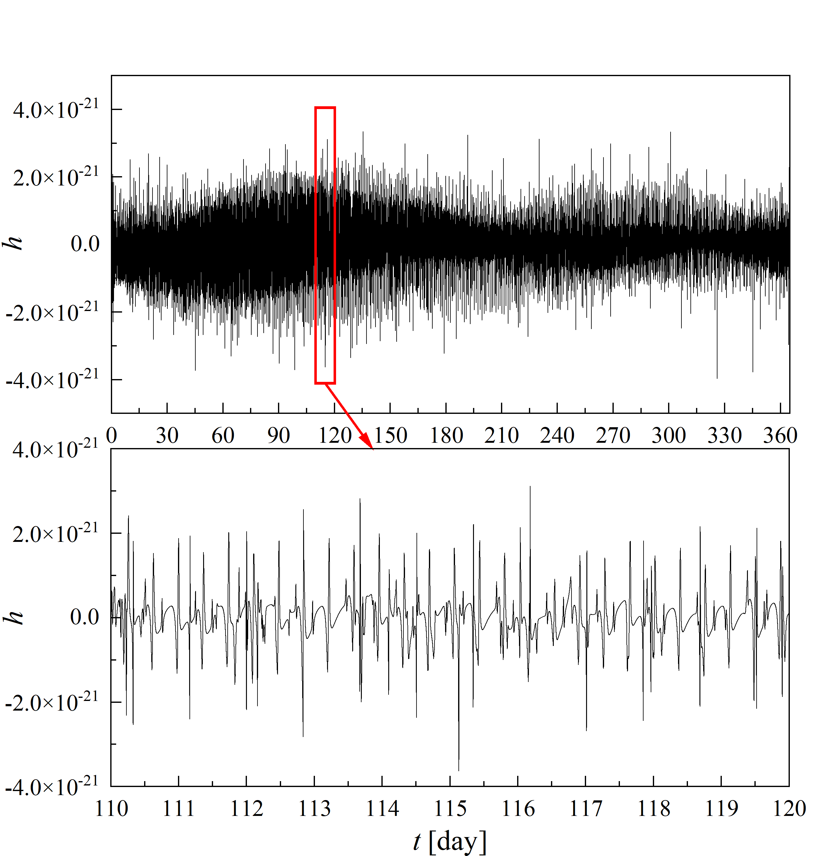
Bursting sources have the potential to form a non-negligible GW background in the millihertz band, given their significant GW radiation (Equations (2)-(7)) and extended lifetime (Equation (8)). Particularly, frequent bursts from multiple sources with low SNR can accumulate to yield a stochastic background noise (see Eqs. (6) and (7)). For example, in Figure 1, we follow the strategy described in Section III and calculate the collective GW signal from bursting BBHs in the Milky Way globular clusters. As shown in this example, the collective bursting signal is a superposition of GW transients, i.e., individual bursts, from various sources, each localized in time and frequency. Additionally, we also include the LISA detector’s response to the bursting GW background, which yields a long-term modulation due to the orbit of LISA around the Sun (see Upper Panel of Figure 1).
The transient nature of bursting signals (see Lower Panel of Figure 1) poses several challenges for existing data analysis strategies, such as the matched filtering method [91, 34], which relies on accurate templates of GW signals and may not perform optimally in fitting bursts [see, e.g., 79, 31, 32]. In particular, GW templates for highly eccentric sources are underdeveloped, which adds to the difficulty of constructing a template bank for the extraction of the signal. Moreover, multiple bursting sources can be present in the detector’s output, which may lead to the misidentification of sources and degeneracy of the fitted parameters.
We note that many efforts have been made to analyze transient events in LIGO data analysis (e.g., power stacking [1], wavelet decomposition [92], and the Q-transform [93, 94]). Furthermore, several studies focused on the transients from highly eccentric EMRIs, which can be possibly seen by LISA [20, 95, 96, 21, 97]. However, the burst detection methods for stellar-mass binaries, particularly when multiple sources’ bursts are present in the datastream simultaneously, remain relatively underdeveloped. In other words, there is uncertainty regarding our ability to identify all bursting sources, even when their signal-to-noise ratio is sufficiently high.
Therefore, we divide the following discussions into two parts, with different criteria for bursting source identification, to demonstrate the potential noise level in future data analysis:
-
1.
Total GW background This criterion includes all the bursting sources regardless of their , assuming that we do not include burst transient templates in the future LISA data analysis. It yields an upper limit for the potential stochastic background level from these sources.
-
2.
Unresolvable noise background This criterion only includes the bursting sources with overall for a yr LISA mission, assuming that we successfully identify all the bursting sources with overall and distinguish them from other signals. It gives a conservative estimation of the noise level from bursting sources.
II.2.2 Stochastic Background Calculation
We follow Barack and Cutler [71] to calculate the stochastic GW background caused by stellar-mass bursting binaries in the LISA band, in which the one-sided noise spectral density is estimated as:
| (11) |
here is the observed frequency, and is the total GW energy density in the corresponding frequency band.
For an eccentric binary, its time domain waveform, , can be decomposed into different harmonics, each with the frequency of [for simplicity, here we rms averaged over the binary inclination, see e.g., 101, 102, 38]:
| (12) |
where
| (13) |
and:
| (14) |
| (15) |
in which is the i-th Bessel function evaluated at .
The energy density of a monochromatic GW signal with frequency can be expressed as [see, e.g., 103]:
| (16) |
where are the amplitude of GW’s two polarizations, and stands for the sky-averaged stain amplitude.
Since the gravitational wave signal from an eccentric source consists of multiple harmonics with different frequencies, the total energy spectral density is a superposition of each harmonic’s contribution. In other words, by combining Equations (12)-(16), we can derive the energy density contribution from all the harmonics below a given frequency, :
| (17) |
Here, we assume the GW source evolves slowly. Thus, the signal does not undergo a significant frequency shift during the observation, and each harmonic is a monochromatic signal with the power concentrates on . We expect that most sources will be consistent with this assumption [e.g., 63, 33]; however, in some cases, the signal may shift in a short timescale, [24, 62], which is beyond the scope of this study.
A key term in the noise spectral density, Eq. (11), is . However, as can be seen from Equation (12)-(17), the number of harmonics making a substantial contribution to the signal rises rapidly as eccentricity reaches extreme values. For example, we may have to consider millions to billions of harmonics when calculating the spectral density of GW signal from a binary with . Consequently, Equation (17) might not always be practical for noise spectral density calculations.
Thus, we further average Equation (17) over a frequency bin to get a smoothed expression of . In particular, for a frequency bin at frequency , each GW harmonic within this bin contributes an energy density of approximately , where , and the number of harmonics included in this bin equals . Therefore, the total energy spectral density at is obtained by summing the energy densities of all these harmonics:
| (18) |
and thus,
| (19) |
Below, we adopt Equation (19) to calculate the energy spectrum of a single bursting source, then sum all the bursting sources’ contributions to get the total GW power spectrum:
| (20) |
For bursting sources at a cosmological distance, we further take into account the redshift [e.g., see 77, 71]:
| (21) |
here is the emitted energy spectrum of the GW sources (i.e., energy per unit comoving volume, unit proper time, and unit emitted frequency).
We note that, in general, there exists a straightforward relationship between the spectrum of the gravitational wave background produced by a cosmological distribution of discrete gravitational wave sources and the present-day comoving number density of remnants, as described by Eq. 5 in Ref. [104]. Realistic examples and further discussions on this relationship can be found in studies such as Refs. [105, 106]. For our cases, however, since the local population can have a non-negligible contribution to the overall GW background level, we include the inhomogeneous spatial distribution and non-equilibrium star formation history in the MCMC simulations afterward (see Section III.1). Therefore, in order to keep consistent, we adopt Equations (20) and (21) as a robust approach to estimate the GW background level across all channels, including cosmological background calculations.
III Simulations of Different Bursting Galactic Sources
III.1 Configuration of the Simulations
As a proof of concept, we adopt the population model in Xuan et al. [33] to generate the parameters of highly eccentric, stellar-mass BBHs in the millihertz band 333Note that for other kinds of bursting compact object binary, such as Double White Dwarfs (DWDs), there exists considerable uncertainty in their orbital evolution due to tidal interaction and mass transfer [see, e.g., 149, 150], particularly for cases involving extreme eccentricity. Therefore, our discussion is limited to BBHs, and we leave the discussion of other populations for future work. Nevertheless, it’s worth noting that the tidal interaction of DWDs tends to circularize the orbit, preventing eccentricity from reaching extreme values [see, e.g., 151, 152]. Additionally, the close approach of bursting DWDs at their pericenter may induce mass transfer and spin interaction, further restricting the lifetime of highly eccentric sources [see, e.g., Fig.4 in 33]. Thus, we suspect a limited population of highly eccentric DWDs and a negligible noise background from bursting DWDs in the millihertz band, even in the presence of external dynamical perturbations.. We consider three regimes that are expected to host eccentric BBHs: Globular Clusters (GCs), Galactic Field, and Galactic Nuclei (GNs). Within each of these regimes, we split the discussion into several specific cases specified below.
In the simulation of BBHs in Globular Clusters and the Galactic Field, we adopt the steady-state approximation, assuming a continuous birth and death of compact object binaries in the universe while keeping the total number of GW sources unchanged. We calibrate our GW power spectrum based on the BBHs merger rate in the universe: [e.g., 108, 45, 109], [51]. Moreover, adopting the galaxy number density of [110], we can use the BBH merger rate in the universe to estimate the merger rate in an averaged galaxy: , .
For the Galactic Nuclei, we consider not only the old population of stars (calibrated using the steady-state approximation and the relation [111, 112]), but also incorporate the non-equilibrium star formation history in the case of the Milky Way center, based on observational results [see, e.g., 113, 114, 115, 116].
We note that the merger rate of BBHs can depend on the star formation history and exceed the estimation in the local universe at high redshift. This phenomenon is especially significant for the globular cluster channel [see, e.g., 117, 118, 119, 120, 121, 122]. Therefore, when calculating the cosmological background of bursting GW sources from GCs, we additionally take into account the change of BBH merger rate as a function of redshift and integrate Equation (21) up to redshift (i.e., Gyr from present), following the merger rate evolution in figure 1 of Ref. [121]. The adopted redshift cutoff is partly justified because represents the epoch of the peak of globular cluster formation rate [118].
For a more detailed description of the population model, see Sections 3.2-3.6 and Appendix A of Ref. [33].
III.2 Stochastic background from the Simulations’ Results
III.2.1 Dynamically formed BBHs in Globular Clusters
Globular clusters are proposed to be a primary channel for the formation of GW mergers. In particular, the dense stellar environment within globular clusters results in various dynamical interactions, including scattering, few-body captures, the Eccentric Kozai-Lidov Mechanism, and Non-EKL triple interactions [see, e.g., 123, 40, 124, 44, 125, 43, 45]. Due to these frequent dynamical interactions, BBHs in globular clusters are anticipated to have non-negligible eccentricity, even within the frequency band of LIGO [see, e.g., 40, 44, 41, 42, 43, 45]. Moreover, since globular clusters widely exist in the universe (e.g., approximately 150 in the Milky Way [126, 127]), we expect a significant number of bursting sources originating from GCs.
For the GW background calculation, we adopt the BBHs eccentricity and semi-major axis distribution from previous studies [see, e.g., figure 4 in 43, for a summary], and assume that all the BBHs have the mass of for simplicity. Using the steady-state approximation, we further average the power spectrum in Equation (20) over the evolution time of GW sources, i.e.,
| (22) |
in which is the merger timescale of a BBH system.
We note that, in Equation (22), , , and are functions of time . As a result, each integral gives the averaged GW power spectrum contribution of a bursting source throughout its lifetime. In the simulation, we initiate each system with the parameters at its formation, evolve the system until it merges, and adjust the collective GW power spectrum by varying the number of systems generated in the MCMC simulation. This adjustment ensures that the product of the number of systems and the inverse of their average lifetime equals the overall merger rate (see Section III.1).
We adopt the spatial distribution of GCs in the Milky Way from Ref. [128]. For simplicity, we assume that the detector’s distance to all GCs in M31 (M33) is 777 (835) kpc, respectively. The cosmological background of bursting BBHs in GCs is determined using Equation (21), with the assumption that the number density of Milky-Way like galaxies is [110].
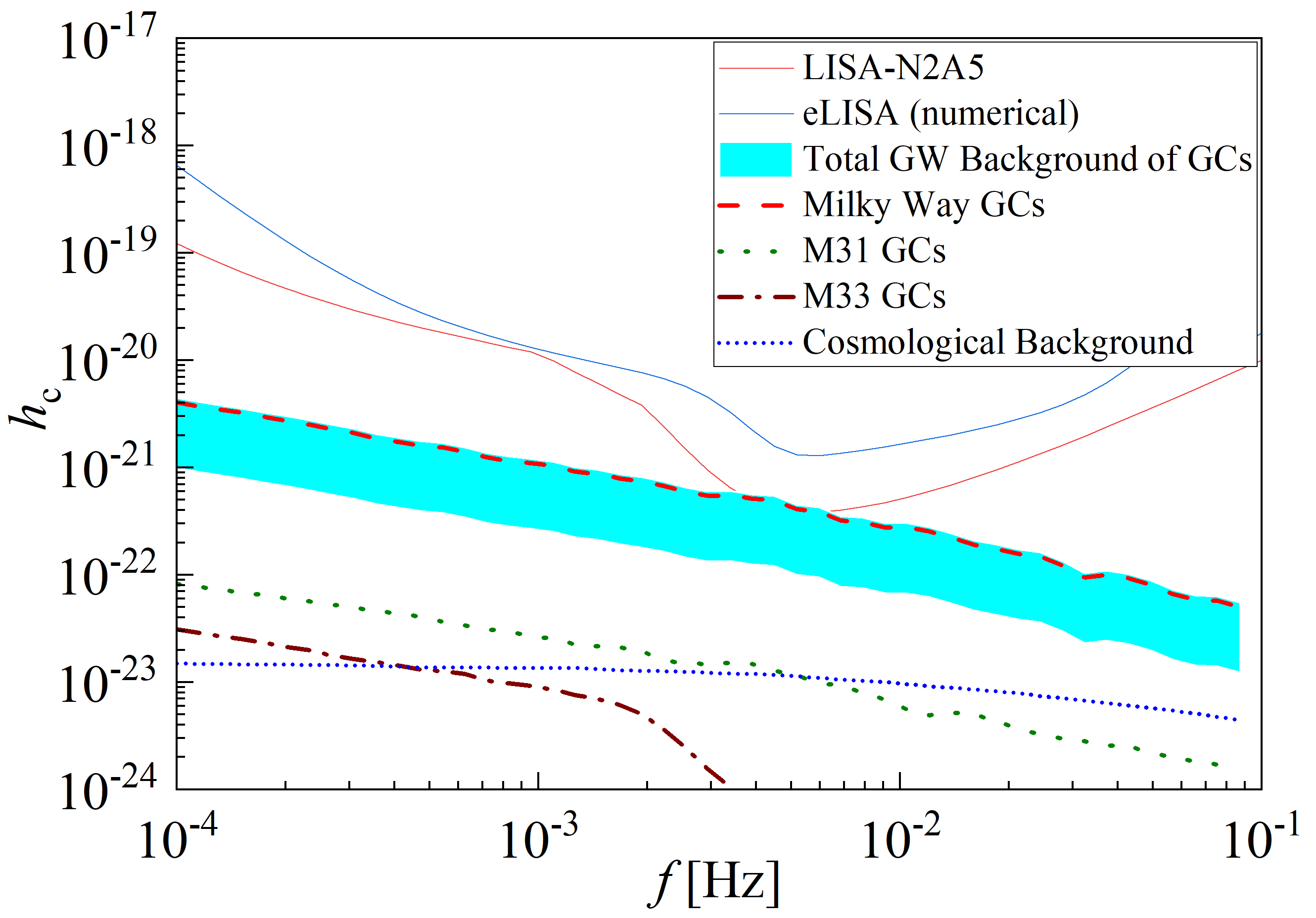
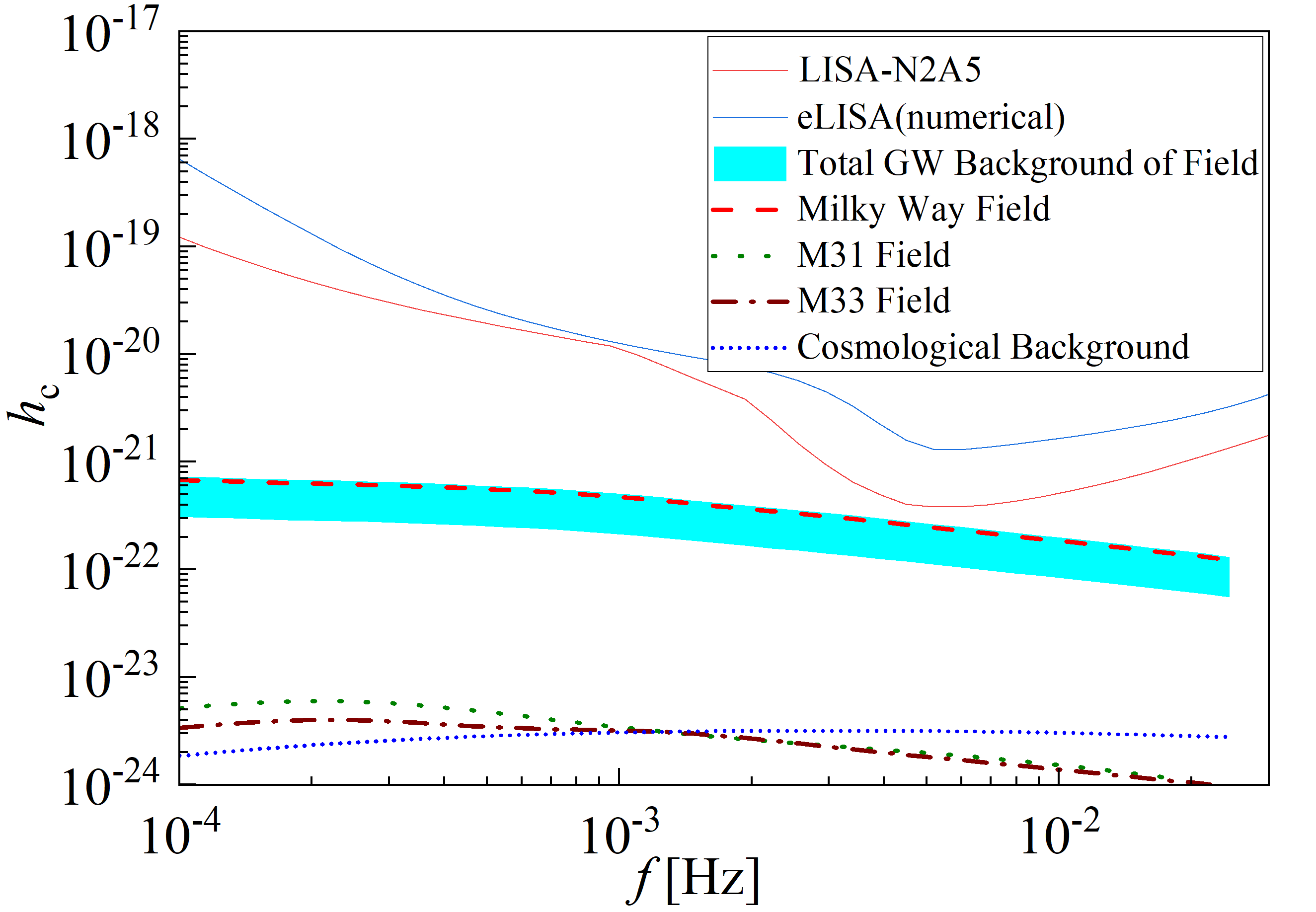
Figure 2, Left Panel, shows the maximum stochastic background from bursting BBHs in the Milky Way GCs (red dashed line), M31 GCs (green dotted line), M33 GCs (brown dashed-dot line), and GCs at a cosmological distance (blue dotted line). The overall GW power spectrum (depicted by the blue-shaded band) is contracted by adding all the sources, for which the maximum (minimum) value corresponds to the maximum (minimum) aforementioned merger rate. As can be seen in Left Panel of Figure 2, bursting BBHs within Milky Way GCs dominate the overall GW power spectrum. Meanwhile, the contributions from the other three channels have comparable levels, approximately two orders of magnitude weaker than Milky Way GCs. Moreover, the total GW background reaches the LISA noise curve at around 5 mHz, which suggests that neglecting these sources in future data analysis could significantly compromise LISA’s sensitivity.
We note that, previous studies [see, e.g., 74, 73, 40] have shown the overall cosmological GW background from stellar-mass BBHs, accounting for all the eccentricity values, is either comparable to or smaller than the millihertz LISA noise level. For our cases, as the highly eccentric binaries represent a subset of the entire BBH population, we anticipate their cosmological GW spectrum level to be lower than the overall background from BBHs and, thus fall below the LISA noise curve. This prediction serves as an upper bound for the cosmological background of bursting sources in the simulation, and turns out to be consistent with the simulation result (depicted by the blue dotted line in Figure 2).
Additionally, the noise background from the unresolvable sources (i.e., the GW spectrum of sources with below 8 for a 4-year LISA mission), is over two orders of magnitude weaker than the LISA sensitivity. Thus, it is omitted here to avoid clutter, and we present this below, see Figure 4.
III.2.2 Fly-by induced, highly eccentric BBHs in the Galactic Field
Recent studies show that external perturbations, such as flybys or galactic tides, can exert a significant influence on the orbital evolution of wide compact object binaries in the galactic field [see, e.g., 129, 51, 52, 53]. Although the isolated wide binaries are not likely to merge due to their large GW merger timescale (sometimes exceeding the Hubble time, as indicated by Equation (9)), the dynamical perturbations from the environment can drive their eccentricity to extreme values, making the BBH system emit GW bursts during pericenter passage, and resulting in a GW merger. Given the substantial number of stars in the galactic field, the fly-by-induced bursting BBHs can significantly contribute to the overall GW background, even if their fraction within the entire stellar population is small.
We follow a similar approach for the GW background calculation as shown in Section III.2.1. In particular, we generate the spacial distribution of wide BBHs according to the density profile of a Milky-Way type galaxy (see Eq. (23)(26) in Ref. [51]). We randomly generate the semi-major axis of BBHs with the log-uniform distribution (from to ), then calculate the fly-by merger rate as a function of semi-major axis [see Eq. (16)(23) in 53]. With a given semi-major axis, there is a critical eccentricity, , for a BBH system to merge before the next fly-by [see Eq. (2) in 53]. Therefore, we randomly generate the initial eccentricity of fly-by induced merger in the range of to , following the thermal distribution .
Following the abovementioned approach, we compute the parameter distribution of fly-by-induced bursting BBHs, then adopt Equation (22) to estimate the overall GW background of Milky Way, M31, and M33, under the steady state approximation. For the cosmological background, we fix the BBHs merger rate for simplicity, and integrate Equation (21) up to to keep consistent with the case of GCs (see Section III.1). As shown in the Right Panel of Figure 2, although the total GW background from bursting BBHs in the galactic field does not reach the LISA noise curve level, it still significantly contributes to the overall GW background.
III.2.3 BBHs in Galactic Nuclei
The galactic nucleus, particularly if hosting an SMBH, can be a promising environment for the formation of stellar-mass bursting BBHs [see, e.g., 38, 108, 58, 130, 131, 60, 63, 132, 133]. For example, consider a stellar-mass BBH system orbiting the SMBH in the galactic nucleus. The EKL mechanism can induce eccentricity excitation in the inner binary’s orbit, potentially driving the eccentricity to extreme values and triggering GW bursts [57, 56, 58, 59, 60, 61, 62, 63]. Consequently, we anticipate a high fraction of bursting BBHs in the galactic center, especially within the Nuclear Star Cluster, where the influence of the SMBH dominates the dynamical environment.
The number of bursting BBHs in the Galactic Nucleus can strongly depend on their formation history. For example, the main population of stars in the Milky Way Galactic Nuclei formed approximately ago [114, 116]. Consequently, this old population of stars may have reached an equilibrium state, resulting in a low rate of compact object binary formation. Therefore, we can use the steady-state approximation and adopt the same approach outlined in Section III.2.1 and III.2.2 to calculate their GW power spectrum.
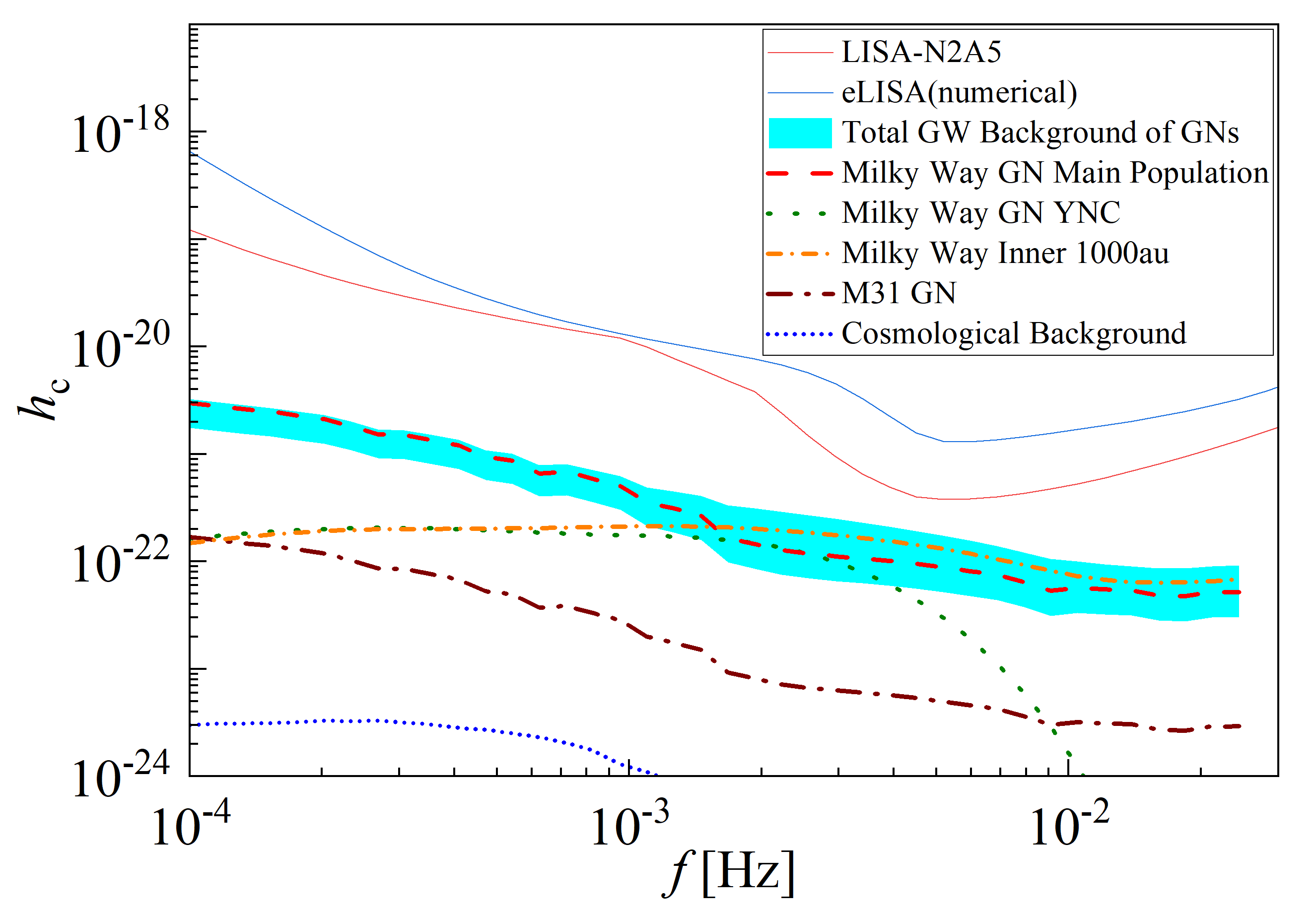
However, observation shows there is a young nuclear star cluster (YNC) at the Milky Way center, which is formed approximately ago [see, e.g., 113, 134, 115, 116]. Moreover, there might be a hidden mass of within the inner au of the Milky Way center [e.g., 135, 136], supported by the observation of stellar motion and the theoretical arguments of the stability of S0-2, [e.g., 137, 138, 139, 140, 141]. In our previous work [33], we carried out Monte-Carlo simulations of these BBHs’ evolution, taking into account the EKL effect up to the octupole level of approximation [142], general relativity precession [e.g., 143], and GW emission [17]. The results indicated that the young population of stars potentially has a much higher fraction of bursting BBHs, especially when the YNC’s age is below the detectable lifetime of bursting sources [see, e.g., Fig.7 in 33].
The summary of the simulation results is presented in Figure 3. For the main population of stars in the Milky Way center, the galactic nuclei of nearby galaxies (M31), and the cosmological background, we follow a similar approach as mentioned in Sections III.2.1 and III.2.2, adopt the steady-state approximation, and use the simulation results in Xuan et al. [33] to calculate their GW background.
However, the steady-state assumption is no longer suitable for the bursting BBHs in the YNC and inner au of the Milky Way center. Thus, we track the time evolution of these populations as a function of the time, assuming that they were born in a starburst. The total GW power spectrum is calculated using Equation (20) and then averaged over the possible age range of the system. The blue-colored region in Figure 3 represents the collective GW power spectrum from all these channels’ contributions. When computing its upper boundary, we sum over the maximum possible GW background level of all these channels. For its lower boundary, we exclude the contribution from bursting BBHs in the inner au, as the existence of this population is highly uncertain.
IV Discussion
Highly eccentric compact object binaries with wide orbits can naturally arise from the dynamical formation of gravitational wave sources. During each pericenter passage, these systems emit significant gravitational waves, potentially resulting in burst signals within the millihertz band. We adopted the analysis from our previous paper [33] and characterized the gravitational wave burst using Equations (2) - (7), detailed in Section II.1, for completeness.
While the population of bursting sources may be large in the Universe, primarily due to their extended lifetime (see Equation (8)-(10)), their GW signals exhibit a transient nature, which poses challenges in the data analysis. In other words, current data analysis approaches may not properly identify bursting gravitational wave sources, even when the overall power of a signal (i.e., SNR) exceeds the conventional detection threshold for circular binaries (see the discussion in Section II.2.1). Therefore, highly eccentric binaries can contribute to a non-negligible stochastic GW background in future millihertz detections (as depicted by the example in Figure 1).
In Section II.2.2, we developed an analytical framework for computing the stochastic GW background from bursting sources. Subsequently, we carried out numerical simulations to determine the GW background from bursting BBHs in different formation channels, utilizing the population model of highly eccentric binaries outlined in Section III.1. Specifically, Figure 2 depicts the example of the GW stochastic background from GCs and the Galactic Fields (left and right panels, respectively), adopting a steady-state approach for the sources’ formation rate. In Figure 3, we also include the fact that a young population of stars has been observed in the center of the Milky Way [134, 144, 145, 115, 135, 116]. This young population implies that the center of our galaxy may deviate from the steady state restriction. Thus, we explore the impact of a young population in the nuclear star cluster on the stochastic background. It produces a comparable contribution to the GW background (see Figure 2, dotted green line). Additionally, there have been observational and theoretical several studies that suggested the existence of about a few thousand of solar mass inwards to S0-2’s orbit [136, 139, 140, 141, 146]. We thus add a population of compact objects inwards to S0-2’s orbit ( au). That may also have a significant contribution to the GW stochastic background.
As depicted in Figures 2-3, highly eccentric BBHs within the Milky Way dominate the stochastic background of GW bursts across all three channels (Globular Cluster, Galactic Field, and Galactic Nuclei), surpassing the contributions from other galaxies and the cosmological background. This pattern indicates that highly eccentric binaries are localized GW sources, like the galactic DWDs.
The dominance of the Milky Way’s contribution, or in other words, the reason for the low level of cosmological background, can be understood by comparing the GW energy of bursting and non-bursting sources at the same frequency band (i.e., with the same pericenter distance , see Equation (2)). According to steady-state approximation, the number of GW sources is proportional to their lifetime, making the total number of bursting sources approximately times the number of circular inspirals formed via dynamical channels (see Equation (10)). However, since highly eccentric sources have lower GW emission power, the energy density contribution of a single bursting source is suppressed by a factor of in the same frequency band (see Equation (6)). Consequently, the overall power spectrum of bursting sources is suppressed by a factor of compared to the contribution from all near-circular sources, implying that their signals are generally weaker, and detection is primarily limited to a short distance.
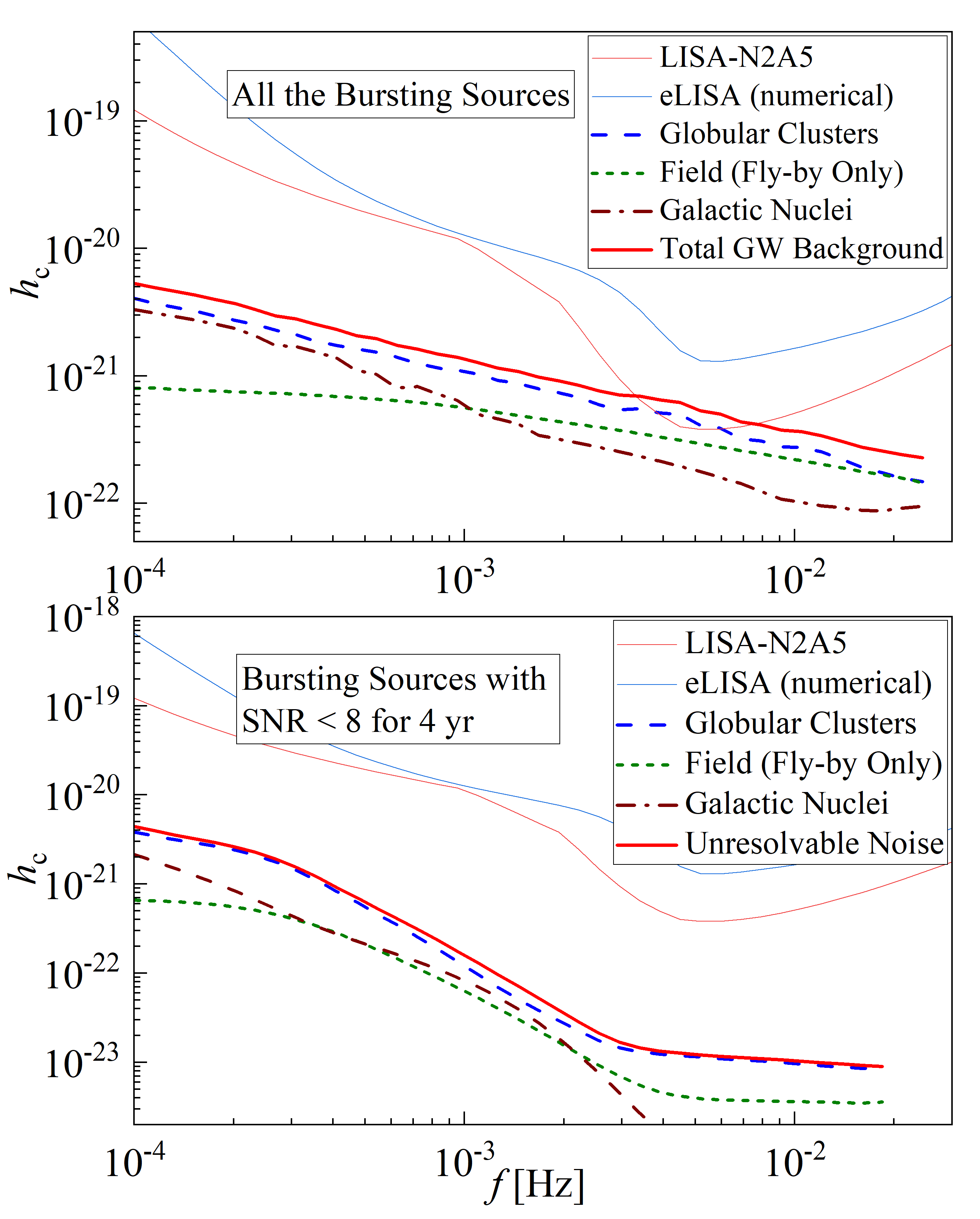
In Figure 4, we summarize the stochastic GW background from bursting BBHs. In particular, Upper Panel shows the maximum level of total GW background from bursting BBHs in Globular Clusters, the Galactic Field, and the Galactic Nuclei, corresponding to the upper boundary of the blue-colored region in Figures 2 and 3. We depict the cumulative contribution of the three channels mentioned above with the solid red line. Bottom Panel represents the unresolvable GW noise background from bursting sources with for a yr LISA mission, which serves as a conservative estimation of the noise level under the assumption that we can identify all the bursting signals with proper templates in the data analysis.
As can be seen in the Figure, highly eccentric, stellar-mass BBHs can have a non-negligible GW background contribution in the LISA detection, potentially exceeding the LISA instrumental noise at mHz (see Upper Panel, in Figure 4). This phenomenon is especially significant if we do not have an effective search strategy for these sources’ GW signals. In the LISA data analysis, if we only use the near-circular GW templates, the GW bursts from these sources will not be identified and will only be considered as a noise background in the detector’s output. Therefore, even with promising , the bursting GW sources will become part of the unresolvable noise background, thus affecting the LISA sensitivity (see Section II.2.1).
However, providing that all the stellar-mass bursting sources are properly identified in the future, the residual noise level is around two orders of magnitude lower than the LISA sensitivity curve, thus having a limited effect on the data analysis (see the Bottom Panel). Considering the abovementioned points, we highlight the importance of searching and identifying bursting GW sources in LISA detection. Particularly, we may need to develop portable GW templates for these sources in the matched filtering or adopt other time-frequency approaches, such as power stacking [1] and the Q-transform [93, 94], to characterize the GW bursts from astrophysical sources in LISA data analysis.
Additionally, in realistic detection, the antenna pattern of LISA undergoes rotation across the sky, causing its response to gravitational waves to change with time. As the bursting BBHs in the Milky Way predominantly contribute to the stochastic background and may have an anisotropic distribution, the amplitude of the GW burst background can vary considerably throughout the year. This observation is consistent with the pattern illustrated in Figure 1 [see, e.g., 147, for a similar case].
We note that the population model used in this study is subject to large uncertainties related to star formation and detailed dynamical evolution. It is intended as a heuristic estimate of the GW background from bursting sources. However, as demonstrated in this paper, the anticipated stochastic background of GW bursts can be significant, even when considering only Milky Way binary black holes. Furthermore, the noise level of GW bursts highly depends on the adopted data analysis strategy in LISA detection. Hence, we emphasize the significance of characterizing stellar-mass GW sources with extreme eccentricity, especially their transient GW signals in the millihertz band.
Acknowledgements.
ZX acknowledges partial support from the Bhaumik Institute for Theoretical Physics summer fellowship. ZX, SN, and EM acknowledge the partial support from NASA ATP 80NSSC20K0505 and from NSF-AST 2206428 grant and thank Howard and Astrid Preston for their generous support. This work was supported by the Science and Technology Facilities Council Grant Number ST/W000903/1 (to BK).References
- East et al. [2013] W. E. East, S. T. McWilliams, J. Levin, and F. Pretorius, Phys. Rev. D 87, 043004 (2013), arXiv:1212.0837 [gr-qc] .
- Samsing et al. [2014] J. Samsing, M. MacLeod, and E. Ramirez-Ruiz, Astrophys. J. 784, 71 (2014), arXiv:1308.2964 [astro-ph.HE] .
- Coughlin et al. [2015] M. Coughlin, P. Meyers, E. Thrane, J. Luo, and N. Christensen, Physical Review D 91 (2015), 10.1103/physrevd.91.063004.
- Gondán et al. [2018a] L. Gondán, B. Kocsis, P. Raffai, and Z. Frei, The Astrophysical Journal 860, 5 (2018a).
- Gondán et al. [2018b] L. Gondán, B. Kocsis, P. Raffai, and Z. Frei, The Astrophysical Journal 855, 34 (2018b).
- Moore et al. [2019] C. J. Moore, D. Gerosa, and A. Klein, Mon. Not. R. Astron. Soc. 488, L94 (2019), arXiv:1905.11998 [astro-ph.HE] .
- Abbott et al. [2021] R. Abbott et al., Astrophys. J. Lett. 913, L7 (2021), arXiv:2010.14533 [astro-ph.HE] .
- The LIGO Scientific Collaboration et al. [2021] The LIGO Scientific Collaboration, the Virgo Collaboration, the KAGRA Collaboration, et al., arXiv e-prints , arXiv:2111.03634 (2021), arXiv:2111.03634 [astro-ph.HE] .
- Zevin et al. [2021] M. Zevin, I. M. Romero-Shaw, K. Kremer, E. Thrane, and P. D. Lasky, The Astrophysical Journal Letters 921, L43 (2021).
- Lower et al. [2018] M. E. Lower, E. Thrane, P. D. Lasky, and R. Smith, Phys. Rev. D 98, 083028 (2018).
- Romero-Shaw et al. [2019] I. M. Romero-Shaw, P. D. Lasky, and E. Thrane, Monthly Notices of the Royal Astronomical Society 490, 5210–5216 (2019).
- et.al. [2019] B. P. A. et.al., The Astrophysical Journal 883, 149 (2019).
- Lenon et al. [2020] A. K. Lenon, A. H. Nitz, and D. A. Brown, Monthly Notices of the Royal Astronomical Society 497, 1966–1971 (2020).
- Romero-Shaw et al. [2020] I. Romero-Shaw, P. D. Lasky, E. Thrane, and J. C. Bustillo, The Astrophysical Journal Letters 903, L5 (2020).
- Gayathri et al. [2022] V. Gayathri, J. Healy, J. Lange, B. O’Brien, M. Szczepanczyk, I. Bartos, M. Campanelli, S. Klimenko, C. Lousto, and R. O’Shaughnessy, “Eccentricity estimate for black hole mergers with numerical relativity simulations,” (2022), arXiv:2009.05461 [astro-ph.HE] .
- Samsing et al. [2022] J. Samsing, I. Bartos, D. J. D’Orazio, Z. Haiman, B. Kocsis, N. W. C. Leigh, B. Liu, M. E. Pessah, and H. Tagawa, Nature 603, 237 (2022), arXiv:2010.09765 [astro-ph.HE] .
- Peters [1964] P. C. Peters, Physical Review 136, 1224 (1964).
- Hinder et al. [2008] I. Hinder, B. Vaishnav, F. Herrmann, D. M. Shoemaker, and P. Laguna, Phys. Rev. D 77, 081502 (2008), arXiv:0710.5167 [gr-qc] .
- Amaro-Seoane et al. [2017] P. Amaro-Seoane et al., arXiv e-prints , arXiv:1702.00786 (2017), arXiv:1702.00786 [astro-ph.IM] .
- Barack and Cutler [2004a] L. Barack and C. Cutler, Phys. Rev. D 69, 082005 (2004a), gr-qc/0310125 .
- Mikóczi et al. [2012] B. Mikóczi, B. Kocsis, P. Forgács, and M. Vasúth, Phys. Rev. D 86, 104027 (2012), arXiv:1206.5786 [gr-qc] .
- Robson et al. [2018] T. Robson, N. J. Cornish, N. Tamanini, and S. Toonen, Phys. Rev. D 98, 064012 (2018), arXiv:1806.00500 [gr-qc] .
- Chen et al. [2019] X. Chen, S. Li, and Z. Cao, Mon. Not. R. Astron. Soc. 485, L141 (2019), arXiv:1703.10543 [astro-ph.HE] .
- Hoang et al. [2019] B.-M. Hoang, S. Naoz, B. Kocsis, W. M. Farr, and J. McIver, Astrophys. J. Lett. 875, L31 (2019), arXiv:1903.00134 [astro-ph.HE] .
- Fang et al. [2019] Y. Fang, X. Chen, and Q.-G. Huang, Astrophys. J. 887, 210 (2019), arXiv:1908.01443 [astro-ph.HE] .
- Tamanini et al. [2020] N. Tamanini, A. Klein, C. Bonvin, E. Barausse, and C. Caprini, Phys. Rev. D 101, 063002 (2020), arXiv:1907.02018 [astro-ph.IM] .
- Torres-Orjuela et al. [2021] A. Torres-Orjuela, P. Amaro Seoane, Z. Xuan, A. J. K. Chua, M. J. B. Rosell, and X. Chen, Phys. Rev. Lett. 127, 041102 (2021), arXiv:2010.15842 [gr-qc] .
- Amaro-Seoane et al. [2022] P. Amaro-Seoane et al., arXiv e-prints , arXiv:2203.06016 (2022), arXiv:2203.06016 [gr-qc] .
- Xuan et al. [2021] Z. Xuan, P. Peng, and X. Chen, Mon. Not. R. Astron. Soc. 502, 4199 (2021), arXiv:2012.00049 [astro-ph.HE] .
- Xuan et al. [2023a] Z. Xuan, S. Naoz, and X. Chen, Phys. Rev. D 107, 043009 (2023a), arXiv:2210.03129 [astro-ph.HE] .
- Loutrel and Yunes [2017] N. Loutrel and N. Yunes, Classical and Quantum Gravity 34, 135011 (2017).
- Loutrel [2020] N. Loutrel, arXiv e-prints , arXiv:2009.11332 (2020), arXiv:2009.11332 [gr-qc] .
- Xuan et al. [2023b] Z. Xuan, S. Naoz, B. Kocsis, and E. Michaely, arXiv e-prints , arXiv:2310.00042 (2023b), arXiv:2310.00042 [astro-ph.HE] .
- Cutler and Flanagan [1994] C. Cutler and É. E. Flanagan, Phys. Rev. D 49, 2658 (1994), arXiv:gr-qc/9402014 [gr-qc] .
- O’Leary et al. [2009a] R. M. O’Leary, B. Kocsis, and A. Loeb, Mon. Not. R. Astron. Soc. 395, 2127 (2009a), arXiv:0807.2638 [astro-ph] .
- Thompson [2011] T. A. Thompson, Astrophys. J. 741, 82 (2011), arXiv:1011.4322 [astro-ph.HE] .
- Aarseth [2012] S. J. Aarseth, Mon. Not. R. Astron. Soc. 422, 841 (2012), arXiv:1202.4688 [astro-ph.SR] .
- Kocsis and Levin [2012] B. Kocsis and J. Levin, Physical Review D 85 (2012), 10.1103/physrevd.85.123005.
- Breivik et al. [2016] K. Breivik, C. L. Rodriguez, S. L. Larson, V. Kalogera, and F. A. Rasio, Astrophys. J. Lett. 830, L18 (2016), arXiv:1606.09558 .
- D’Orazio and Samsing [2018] D. J. D’Orazio and J. Samsing, Mon. Not. R. Astron. Soc. 481, 4775 (2018), arXiv:1805.06194 [astro-ph.HE] .
- Zevin et al. [2019] M. Zevin, J. Samsing, C. Rodriguez, C.-J. Haster, and E. Ramirez-Ruiz, The Astrophysical Journal 871, 91 (2019).
- Samsing et al. [2019] J. Samsing, A. S. Hamers, and J. G. Tyles, Phys. Rev. D 100, 043010 (2019), arXiv:1906.07189 [astro-ph.HE] .
- Martinez et al. [2020] M. A. S. Martinez, G. Fragione, K. Kremer, S. Chatterjee, C. L. Rodriguez, J. Samsing, C. S. Ye, N. C. Weatherford, M. Zevin, S. Naoz, and F. A. Rasio, Astrophys. J. 903, 67 (2020), arXiv:2009.08468 [astro-ph.GA] .
- Antonini and Gieles [2020] F. Antonini and M. Gieles, Mon. Not. R. Astron. Soc. 492, 2936 (2020), arXiv:1906.11855 [astro-ph.HE] .
- Kremer et al. [2020] K. Kremer, C. S. Ye, N. Z. Rui, N. C. Weatherford, S. Chatterjee, G. Fragione, C. L. Rodriguez, M. Spera, and F. A. Rasio, The Astrophysical Journal Supplement Series 247, 48 (2020).
- Winter-Granić et al. [2023] M. Winter-Granić, C. Petrovich, and V. Peña-Donaire, “Binary mergers in the centers of galaxies: synergy between stellar flybys and tidal fields,” (2023), arXiv:2312.17319 [astro-ph.GA] .
- Gondán and Kocsis [2021] L. Gondán and B. Kocsis, Mon. Not. R. Astron. Soc. 506, 1665 (2021), arXiv:2011.02507 [astro-ph.HE] .
- Tagawa et al. [2021] H. Tagawa, B. Kocsis, Z. Haiman, I. Bartos, K. Omukai, and J. Samsing, Astrophys. J. Lett. 907, L20 (2021), arXiv:2010.10526 [astro-ph.HE] .
- Muñoz et al. [2022] D. J. Muñoz, N. C. Stone, C. Petrovich, and F. A. Rasio, arXiv e-prints , arXiv:2204.06002 (2022), arXiv:2204.06002 [astro-ph.HE] .
- Gautham Bhaskar et al. [2023] H. Gautham Bhaskar, G. Li, and D. Lin, arXiv e-prints , arXiv:2303.12539 (2023), arXiv:2303.12539 [astro-ph.HE] .
- Michaely and Perets [2019] E. Michaely and H. B. Perets, Astrophys. J. Lett. 887, L36 (2019), arXiv:1902.01864 [astro-ph.SR] .
- Michaely and Perets [2020] E. Michaely and H. B. Perets, Mon. Not. R. Astron. Soc. 498, 4924 (2020), arXiv:2008.01094 [astro-ph.HE] .
- Michaely and Naoz [2022] E. Michaely and S. Naoz, Astrophys. J. 936, 184 (2022), arXiv:2205.15040 [astro-ph.HE] .
- Kozai [1962] Y. Kozai, Astron. J. 67, 591 (1962).
- Lidov [1962] M. L. Lidov, Planetary and Space Sci. 9, 719 (1962).
- Naoz [2016] S. Naoz, Annu. Rev. Astron. Astrophys. 54, 441 (2016), arXiv:1601.07175 [astro-ph.EP] .
- Wen [2003] L. Wen, Astrophys. J. 598, 419 (2003), arXiv:astro-ph/0211492 [astro-ph] .
- Hoang et al. [2018] B.-M. Hoang, S. Naoz, B. Kocsis, F. A. Rasio, and F. Dosopoulou, Astrophys. J. 856, 140 (2018), arXiv:1706.09896 [astro-ph.HE] .
- Hamers [2018] A. S. Hamers, Mon. Not. R. Astron. Soc. 476, 4139 (2018), arXiv:1802.05716 [astro-ph.SR] .
- Stephan et al. [2019] A. P. Stephan, S. Naoz, A. M. Ghez, M. R. Morris, A. Ciurlo, T. Do, K. Breivik, S. Coughlin, and C. L. Rodriguez, Astrophys. J. 878, 58 (2019), arXiv:1903.00010 [astro-ph.SR] .
- Bub and Petrovich [2020] M. W. Bub and C. Petrovich, Astrophys. J. 894, 15 (2020), arXiv:1910.02079 [astro-ph.HE] .
- Deme et al. [2020] B. Deme, B.-M. Hoang, S. Naoz, and B. Kocsis, The Astrophysical Journal 901, 125 (2020).
- Wang et al. [2021] H. Wang, A. P. Stephan, S. Naoz, B.-M. Hoang, and K. Breivik, Astrophys. J. 917, 76 (2021), arXiv:2010.15841 [astro-ph.HE] .
- Nelemans et al. [2004] G. Nelemans, L. R. Yungelson, and S. F. Portegies Zwart, Monthly Notices of the Royal Astronomical Society 349, 181 (2004), https://academic.oup.com/mnras/article-pdf/349/1/181/11180320/349-1-181.pdf .
- Nissanke et al. [2012a] S. Nissanke, M. Vallisneri, G. Nelemans, and T. A. Prince, Astrophys. J. 758, 131 (2012a), arXiv:1201.4613 [astro-ph.GA] .
- Klein et al. [2016a] A. Klein, E. Barausse, A. Sesana, A. Petiteau, E. Berti, S. Babak, J. Gair, S. Aoudia, I. Hinder, F. Ohme, and B. Wardell, Phys. Rev. D 93, 024003 (2016a), arXiv:1511.05581 [gr-qc] .
- Lamberts et al. [2018] A. Lamberts, S. Garrison-Kimmel, P. F. Hopkins, E. Quataert, J. S. Bullock, C. A. Faucher-Giguère, A. Wetzel, D. Kereš, K. Drango, and R. E. Sand erson, Mon. Not. R. Astron. Soc. 480, 2704 (2018), arXiv:1801.03099 [astro-ph.GA] .
- Huerta et al. [2015] E. A. Huerta, S. T. McWilliams, J. R. Gair, and S. R. Taylor, Phys. Rev. D 92, 063010 (2015).
- Kelley et al. [2017] L. Z. Kelley, L. Blecha, L. Hernquist, A. Sesana, and S. R. Taylor, Monthly Notices of the Royal Astronomical Society 471, 4508 (2017), https://academic.oup.com/mnras/article-pdf/471/4/4508/19609079/stx1638.pdf .
- Chen et al. [2017] S. Chen, A. Sesana, and W. Del Pozzo, Mon. Not. R. Astron. Soc. 470, 1738 (2017), arXiv:1612.00455 [astro-ph.CO] .
- Barack and Cutler [2004b] L. Barack and C. Cutler, Phys. Rev. D 70, 122002 (2004b), arXiv:gr-qc/0409010 [gr-qc] .
- Adams and Cornish [2014] M. R. Adams and N. J. Cornish, Phys. Rev. D 89, 022001 (2014), arXiv:1307.4116 [gr-qc] .
- Nishizawa et al. [2016] A. Nishizawa, E. Berti, A. Klein, and A. Sesana, Physical Review D 94 (2016), 10.1103/physrevd.94.064020.
- Sesana [2016] A. Sesana, Phys. Rev. Lett. 116, 231102 (2016), arXiv:1602.06951 [gr-qc] .
- Boileau et al. [2021] G. Boileau, A. Lamberts, N. Christensen, N. J. Cornish, and R. Meyer, Mon. Not. R. Astron. Soc. 508, 803 (2021), arXiv:2105.04283 [gr-qc] .
- Naoz et al. [2022] S. Naoz, S. C. Rose, E. Michaely, D. Melchor, E. Ramirez-Ruiz, B. Mockler, and J. D. Schnittman, Astrophys. J. Lett. 927, L18 (2022), arXiv:2202.12303 [astro-ph.HE] .
- Naoz and Haiman [2023] S. Naoz and Z. Haiman, arXiv e-prints , arXiv:2307.11149 (2023), arXiv:2307.11149 [astro-ph.HE] .
- Agazie et al. [2023] G. Agazie, A. Anumarlapudi, A. M. Archibald, Z. Arzoumanian, P. T. Baker, B. Bécsy, L. Blecha, A. Brazier, P. R. Brook, S. Burke-Spolaor, R. Burnette, R. Case, M. Charisi, S. Chatterjee, K. Chatziioannou, B. D. Cheeseboro, S. Chen, T. Cohen, J. M. Cordes, N. J. Cornish, F. Crawford, H. T. Cromartie, K. Crowter, C. J. Cutler, M. E. DeCesar, D. DeGan, P. B. Demorest, H. Deng, T. Dolch, B. Drachler, J. A. Ellis, E. C. Ferrara, W. Fiore, E. Fonseca, G. E. Freedman, N. Garver-Daniels, P. A. Gentile, K. A. Gersbach, J. Glaser, D. C. Good, K. Gültekin, J. S. Hazboun, S. Hourihane, K. Islo, R. J. Jennings, A. D. Johnson, M. L. Jones, A. R. Kaiser, D. L. Kaplan, L. Z. Kelley, M. Kerr, J. S. Key, T. C. Klein, N. Laal, M. T. Lam, W. G. Lamb, T. J. W. Lazio, N. Lewandowska, T. B. Littenberg, T. Liu, A. Lommen, D. R. Lorimer, J. Luo, R. S. Lynch, C.-P. Ma, D. R. Madison, M. A. Mattson, A. McEwen, J. W. McKee, M. A. McLaughlin, N. McMann, B. W. Meyers, P. M. Meyers, C. M. F. Mingarelli, A. Mitridate, P. Natarajan, C. Ng, D. J. Nice, S. K. Ocker, K. D. Olum, T. T. Pennucci, B. B. P. Perera, P. Petrov, N. S. Pol, H. A. Radovan, S. M. Ransom, P. S. Ray, J. D. Romano, S. C. Sardesai, A. Schmiedekamp, C. Schmiedekamp, K. Schmitz, L. Schult, B. J. Shapiro-Albert, X. Siemens, J. Simon, M. S. Siwek, I. H. Stairs, D. R. Stinebring, K. Stovall, J. P. Sun, A. Susobhanan, J. K. Swiggum, J. Taylor, S. R. Taylor, J. E. Turner, C. Unal, M. Vallisneri, R. van Haasteren, S. J. Vigeland, H. M. Wahl, Q. Wang, C. A. Witt, O. Young, and T. N. Collaboration, The Astrophysical Journal Letters 951, L8 (2023).
- Tai et al. [2014] K. S. Tai, S. T. McWilliams, and F. Pretorius, Physical Review D 90 (2014), 10.1103/physrevd.90.103001.
- Spadaro et al. [2023] A. Spadaro, R. Buscicchio, D. Vetrugno, A. Klein, D. Gerosa, S. Vitale, R. Dolesi, W. J. Weber, and M. Colpi, “Glitch systematics on the observation of massive black-hole binaries with lisa,” (2023), arXiv:2306.03923 [gr-qc] .
- Armano et al. [2016] M. Armano, H. Audley, G. Auger, J. T. Baird, M. Bassan, P. Binetruy, M. Born, D. Bortoluzzi, N. Brandt, M. Caleno, L. Carbone, A. Cavalleri, A. Cesarini, G. Ciani, G. Congedo, A. M. Cruise, K. Danzmann, M. de Deus Silva, R. De Rosa, M. Diaz-Aguiló, L. Di Fiore, I. Diepholz, G. Dixon, R. Dolesi, N. Dunbar, L. Ferraioli, V. Ferroni, W. Fichter, E. D. Fitzsimons, R. Flatscher, M. Freschi, A. F. García Marín, C. García Marirrodriga, R. Gerndt, L. Gesa, F. Gibert, D. Giardini, R. Giusteri, F. Guzmán, A. Grado, C. Grimani, A. Grynagier, J. Grzymisch, I. Harrison, G. Heinzel, M. Hewitson, D. Hollington, D. Hoyland, M. Hueller, H. Inchauspé, O. Jennrich, P. Jetzer, U. Johann, B. Johlander, N. Karnesis, B. Kaune, N. Korsakova, C. J. Killow, J. A. Lobo, I. Lloro, L. Liu, J. P. López-Zaragoza, R. Maarschalkerweerd, D. Mance, V. Martín, L. Martin-Polo, J. Martino, F. Martin-Porqueras, S. Madden, I. Mateos, P. W. McNamara, J. Mendes, L. Mendes, A. Monsky, D. Nicolodi, M. Nofrarias, S. Paczkowski, M. Perreur-Lloyd, A. Petiteau, P. Pivato, E. Plagnol, P. Prat, U. Ragnit, B. Raïs, J. Ramos-Castro, J. Reiche, D. I. Robertson, H. Rozemeijer, F. Rivas, G. Russano, J. Sanjuán, P. Sarra, A. Schleicher, D. Shaul, J. Slutsky, C. F. Sopuerta, R. Stanga, F. Steier, T. Sumner, D. Texier, J. I. Thorpe, C. Trenkel, M. Tröbs, H. B. Tu, D. Vetrugno, S. Vitale, V. Wand, G. Wanner, H. Ward, C. Warren, P. J. Wass, D. Wealthy, W. J. Weber, L. Wissel, A. Wittchen, A. Zambotti, C. Zanoni, T. Ziegler, and P. Zweifel, Phys. Rev. Lett. 116, 231101 (2016).
- Armano et al. [2018] M. Armano, H. Audley, J. Baird, P. Binetruy, M. Born, D. Bortoluzzi, E. Castelli, A. Cavalleri, A. Cesarini, A. M. Cruise, K. Danzmann, M. de Deus Silva, I. Diepholz, G. Dixon, R. Dolesi, L. Ferraioli, V. Ferroni, E. D. Fitzsimons, M. Freschi, L. Gesa, F. Gibert, D. Giardini, R. Giusteri, C. Grimani, J. Grzymisch, I. Harrison, G. Heinzel, M. Hewitson, D. Hollington, D. Hoyland, M. Hueller, H. Inchauspé, O. Jennrich, P. Jetzer, N. Karnesis, B. Kaune, N. Korsakova, C. J. Killow, J. A. Lobo, I. Lloro, L. Liu, J. P. López-Zaragoza, R. Maarschalkerweerd, D. Mance, N. Meshksar, V. Martín, L. Martin-Polo, J. Martino, F. Martin-Porqueras, I. Mateos, P. W. McNamara, J. Mendes, L. Mendes, M. Nofrarias, S. Paczkowski, M. Perreur-Lloyd, A. Petiteau, P. Pivato, E. Plagnol, J. Ramos-Castro, J. Reiche, D. I. Robertson, F. Rivas, G. Russano, J. Slutsky, C. F. Sopuerta, T. Sumner, D. Texier, J. I. Thorpe, D. Vetrugno, S. Vitale, G. Wanner, H. Ward, P. J. Wass, W. J. Weber, L. Wissel, A. Wittchen, and P. Zweifel, Phys. Rev. Lett. 120, 061101 (2018).
- Babak et al. [2023] S. Babak, C. Caprini, D. G. Figueroa, N. Karnesis, P. Marcoccia, G. Nardini, M. Pieroni, A. Ricciardone, A. Sesana, and J. Torrado, J. Cosmology Astropart. Phys. 2023, 034 (2023), arXiv:2304.06368 [astro-ph.CO] .
- Chen and Amaro-Seoane [2017] X. Chen and P. Amaro-Seoane, Astrophys. J. Lett. 842, L2 (2017), arXiv:1702.08479 [astro-ph.HE] .
- Zhao and Lu [2021] Y. Zhao and Y. Lu, Mon. Not. R. Astron. Soc. 500, 1421 (2021), arXiv:2009.01436 [astro-ph.HE] .
- Note [1] Note that we omit an order unity factor of , following our previous work, [33].
- Note [2] The peak GW frequency of eccentric sources is often estimated as [35]. A more detailed expression of the peak frequency can also be found in Refs. [57, 148]. For consistency with other definitions in our previous treatment [33], we adopt , which differs by an order of unity.
- Klein et al. [2016b] A. Klein, E. Barausse, A. Sesana, A. Petiteau, E. Berti, S. Babak, J. Gair, S. Aoudia, I. Hinder, F. Ohme, and B. Wardell, Phys. Rev. D 93, 024003 (2016b), arXiv:1511.05581 [gr-qc] .
- Robson et al. [2019] T. Robson, N. J. Cornish, and C. Liu, Classical and Quantum Gravity 36, 105011 (2019), arXiv:1803.01944 [astro-ph.HE] .
- Nissanke et al. [2012b] S. Nissanke, M. Vallisneri, G. Nelemans, and T. A. Prince, Astrophys. J. 758, 131 (2012b), arXiv:1201.4613 [astro-ph.GA] .
- Finn and Chernoff [1993] L. S. Finn and D. F. Chernoff, Phys. Rev. D47, 2198 (1993), arXiv:gr-qc/9301003 .
- Klimenko and Mitselmakher [2004] S. Klimenko and G. Mitselmakher, Classical and Quantum Gravity 21, S1819 (2004).
- Bassetti et al. [2005] M. J. Bassetti, A. N. Chatterjee, N. Aluru, and D. J. Beebe, Journal of Microelectromechanical Systems 14, 1198 (2005).
- Tai et al. [2014] K. S. Tai, S. T. McWilliams, and F. Pretorius, Phys. Rev. D 90, 103001 (2014), arXiv:1403.7754 [gr-qc] .
- Cornish and Larson [2003] N. J. Cornish and S. L. Larson, Phys. Rev. D 67, 103001 (2003), arXiv:astro-ph/0301548 [astro-ph] .
- Porter and Sesana [2010] E. K. Porter and A. Sesana, “Eccentric massive black hole binaries in lisa i : The detection capabilities of circular templates,” (2010), arXiv:1005.5296 [gr-qc] .
- Fan et al. [2022] H.-M. Fan, S. Zhong, Z.-C. Liang, Z. Wu, J.-d. Zhang, and Y.-M. Hu, Phys. Rev. D 106, 124028 (2022), arXiv:2209.13387 [gr-qc] .
- [98] .
- Cutler [1998] C. Cutler, Phys. Rev. D 57, 7089 (1998), arXiv:gr-qc/9703068 [gr-qc] .
- Cornish and Rubbo [2003] N. J. Cornish and L. J. Rubbo, Phys. Rev. D 67, 022001 (2003).
- Peters and Mathews [1963] P. C. Peters and J. Mathews, Physical Review 131, 435 (1963).
- O’Leary et al. [2009b] R. M. O’Leary, B. Kocsis, and A. Loeb, Mon. Not. R. Astron. Soc. 395, 2127 (2009b), arXiv:0807.2638 .
- Maggiore [2000] M. Maggiore, Physics Reports 331, 283 (2000).
- Phinney [1989] E. S. Phinney, in NATO Advanced Science Institutes (ASI) Series C, NATO Advanced Science Institutes (ASI) Series C, Vol. 290, edited by F. Meyer (1989) p. 457.
- Kocsis and Sesana [2011] B. Kocsis and A. Sesana, Mon. Not. R. Astron. Soc. 411, 1467 (2011), arXiv:1002.0584 [astro-ph.CO] .
- Kocsis et al. [2012] B. Kocsis, A. Ray, and S. Portegies Zwart, Astrophys. J. 752, 67 (2012), arXiv:1110.6172 [astro-ph.GA] .
- Note [3] Note that for other kinds of bursting compact object binary, such as Double White Dwarfs (DWDs), there exists considerable uncertainty in their orbital evolution due to tidal interaction and mass transfer [see, e.g., 149, 150], particularly for cases involving extreme eccentricity. Therefore, our discussion is limited to BBHs, and we leave the discussion of other populations for future work. Nevertheless, it’s worth noting that the tidal interaction of DWDs tends to circularize the orbit, preventing eccentricity from reaching extreme values [see, e.g., 151, 152]. Additionally, the close approach of bursting DWDs at their pericenter may induce mass transfer and spin interaction, further restricting the lifetime of highly eccentric sources [see, e.g., Fig.4 in 33]. Thus, we suspect a limited population of highly eccentric DWDs and a negligible noise background from bursting DWDs in the millihertz band, even in the presence of external dynamical perturbations.
- Rodriguez et al. [2016] C. L. Rodriguez, C.-J. Haster, S. Chatterjee, V. Kalogera, and F. A. Rasio, Astrophys. J. Lett. 824, L8 (2016), arXiv:1604.04254 [astro-ph.HE] .
- Antonini and Gieles [2020] F. Antonini and M. Gieles, Physical Review D 102 (2020), 10.1103/physrevd.102.123016.
- Conselice et al. [2005] C. J. Conselice, J. A. Blackburne, and C. Papovich, The Astrophysical Journal 620, 564 (2005).
- Merritt [1999] D. Merritt, “Black holes and galaxy evolution,” (1999), arXiv:astro-ph/9910546 [astro-ph] .
- Kormendy and Ho [2013] J. Kormendy and L. C. Ho, Annu. Rev. Astron. Astrophys. 51, 511 (2013), arXiv:1304.7762 [astro-ph.CO] .
- Paumard et al. [2006] T. Paumard, R. Genzel, F. Martins, S. Nayakshin, A. M. Beloborodov, Y. Levin, S. Trippe, F. Eisenhauer, T. Ott, S. Gillessen, R. Abuter, J. Cuadra, T. Alexander, and A. Sternberg, Astrophys. J. 643, 1011 (2006), arXiv:astro-ph/0601268 [astro-ph] .
- Lu et al. [2008] J. R. Lu, A. M. Ghez, S. D. Hornstein, M. R. Morris, E. E. Becklin, and K. Matthews, The Astrophysical Journal 690, 1463 (2008).
- Do et al. [2013] T. Do, J. R. Lu, A. M. Ghez, M. R. Morris, S. Yelda, G. D. Martinez, S. A. Wright, and K. Matthews, Astrophys. J. 764, 154 (2013), arXiv:1301.0539 [astro-ph.SR] .
- Chen et al. [2023] Z. Chen, T. Do, A. M. Ghez, M. W. Hosek, A. Feldmeier-Krause, D. S. Chu, R. O. Bentley, J. R. Lu, and M. R. Morris, Astrophys. J. 944, 79 (2023), arXiv:2212.01397 [astro-ph.GA] .
- Zwart and McMillan [1999] S. F. P. Zwart and S. L. W. McMillan, The Astrophysical Journal 528, L17 (1999).
- Gnedin et al. [2014] O. Y. Gnedin, J. P. Ostriker, and S. Tremaine, The Astrophysical Journal 785, 71 (2014).
- Rodriguez et al. [2015] C. L. Rodriguez, M. Morscher, B. Pattabiraman, S. Chatterjee, C.-J. Haster, and F. A. Rasio, Phys. Rev. Lett. 115, 051101 (2015).
- Rodriguez et al. [2016] C. L. Rodriguez, S. Chatterjee, and F. A. Rasio, Phys. Rev. D 93, 084029 (2016).
- Fragione and Kocsis [2018] G. Fragione and B. Kocsis, Phys. Rev. Lett. 121, 161103 (2018), arXiv:1806.02351 [astro-ph.GA] .
- Fragione et al. [2018] G. Fragione, F. Antonini, and O. Y. Gnedin, Monthly Notices of the Royal Astronomical Society 475, 5313 (2018), https://academic.oup.com/mnras/article-pdf/475/4/5313/24106688/sty183.pdf .
- Banerjee et al. [2010] S. Banerjee, H. Baumgardt, and P. Kroupa, Mon. Not. R. Astron. Soc. 402, 371 (2010), arXiv:0910.3954 [astro-ph.SR] .
- Samsing [2018] J. Samsing, Phys. Rev. D 97, 103014 (2018), arXiv:1711.07452 [astro-ph.HE] .
- Fragione et al. [2019] G. Fragione, E. Grishin, N. W. C. Leigh, H. B. Perets, and R. Perna, Mon. Not. R. Astron. Soc. 488, 47 (2019), arXiv:1811.10627 [astro-ph.GA] .
- Harris [1996] W. E. Harris, Astron. J. 112, 1487 (1996).
- Baumgardt and Hilker [2018] H. Baumgardt and M. Hilker, Mon. Not. R. Astron. Soc. 478, 1520 (2018), arXiv:1804.08359 [astro-ph.GA] .
- Arakelyan et al. [2018] N. R. Arakelyan, S. V. Pilipenko, and N. I. Libeskind, Monthly Notices of the Royal Astronomical Society 481, 918 (2018).
- Kaib and Raymond [2014] N. A. Kaib and S. N. Raymond, Astrophys. J. 782, 60 (2014), arXiv:1309.3272 [astro-ph.SR] .
- Hoang et al. [2019] B.-M. Hoang, S. Naoz, B. Kocsis, W. M. Farr, and J. McIver, The Astrophysical Journal 875, L31 (2019).
- Trani et al. [2019] A. A. Trani, M. Spera, N. W. C. Leigh, and M. S. Fujii, Astrophys. J. 885, 135 (2019), arXiv:1904.07879 [astro-ph.GA] .
- Arca Sedda et al. [2023] M. Arca Sedda, S. Naoz, and B. Kocsis, Universe 9, 138 (2023), arXiv:2302.14071 [astro-ph.GA] .
- Zhang and Chen [2024] Z. Zhang and X. Chen, arXiv e-prints , arXiv:2402.02178 (2024), arXiv:2402.02178 [astro-ph.HE] .
- Lu et al. [2006] J. R. Lu, A. M. Ghez, S. D. Hornstein, M. Morris, K. Matthews, D. J. Thompson, and E. E. Becklin, in Journal of Physics Conference Series, Journal of Physics Conference Series, Vol. 54 (2006) pp. 279–287.
- Do et al. [2019] T. Do, A. Hees, A. Ghez, G. D. Martinez, D. S. Chu, S. Jia, S. Sakai, J. R. Lu, A. K. Gautam, K. K. O’Neil, E. E. Becklin, M. R. Morris, K. Matthews, S. Nishiyama, R. Campbell, S. Chappell, Z. Chen, A. Ciurlo, A. Dehghanfar, E. Gallego-Cano, W. E. Kerzendorf, J. E. Lyke, S. Naoz, H. Saida, R. Schödel, M. Takahashi, Y. Takamori, G. Witzel, and P. Wizinowich, Science 365, 664 (2019), arXiv:1907.10731 [astro-ph.GA] .
- GRAVITY Collaboration et al. [2020] GRAVITY Collaboration, R. Abuter, A. Amorim, M. Bauböck, J. P. Berger, H. Bonnet, W. Brandner, V. Cardoso, Y. Clénet, P. T. de Zeeuw, J. Dexter, A. Eckart, F. Eisenhauer, N. M. Förster Schreiber, P. Garcia, F. Gao, E. Gendron, R. Genzel, S. Gillessen, M. Habibi, X. Haubois, T. Henning, S. Hippler, M. Horrobin, A. Jiménez-Rosales, L. Jochum, L. Jocou, A. Kaufer, P. Kervella, S. Lacour, V. Lapeyrère, J. B. Le Bouquin, P. Léna, M. Nowak, T. Ott, T. Paumard, K. Perraut, G. Perrin, O. Pfuhl, G. Rodríguez-Coira, J. Shangguan, S. Scheithauer, J. Stadler, O. Straub, C. Straubmeier, E. Sturm, L. J. Tacconi, F. Vincent, S. von Fellenberg, I. Waisberg, F. Widmann, E. Wieprecht, E. Wiezorrek, J. Woillez, S. Yazici, and G. Zins, Astron. Astrophys. 636, L5 (2020), arXiv:2004.07187 [astro-ph.GA] .
- Chu et al. [2018] D. S. Chu, T. Do, A. Hees, A. Ghez, S. Naoz, G. Witzel, S. Sakai, S. Chappell, A. K. Gautam, J. R. Lu, and K. Matthews, Astrophys. J. 854, 12 (2018), arXiv:1709.04890 [astro-ph.SR] .
- Chu et al. [2023] D. S. Chu, T. Do, A. Ghez, A. K. Gautam, A. Ciurlo, K. K. O’neil, M. W. Hosek, A. Hees, S. Naoz, S. Sakai, J. R. Lu, Z. Chen, R. O. Bentley, E. E. Becklin, and K. Matthews, Astrophys. J. 948, 94 (2023), arXiv:2303.16977 [astro-ph.GA] .
- Naoz et al. [2020] S. Naoz, C. M. Will, E. Ramirez-Ruiz, A. Hees, A. M. Ghez, and T. Do, Astrophys. J. Lett. 888, L8 (2020), arXiv:1912.04910 [astro-ph.GA] .
- Zhang et al. [2023] E. Zhang, S. Naoz, and C. M. Will, Astrophys. J. 952, 103 (2023), arXiv:2301.08271 [astro-ph.GA] .
- Will et al. [2023] C. M. Will, S. Naoz, A. Hees, A. Tucker, E. Zhang, T. Do, and A. Ghez, arXiv e-prints , arXiv:2307.16646 (2023), arXiv:2307.16646 [astro-ph.GA] .
- Naoz et al. [2013a] S. Naoz, W. M. Farr, Y. Lithwick, F. A. Rasio, and J. Teyssandier, Mon. Not. R. Astron. Soc. 431, 2155 (2013a), arXiv:1107.2414 [astro-ph.EP] .
- Naoz et al. [2013b] S. Naoz, B. Kocsis, A. Loeb, and N. Yunes, Astrophys. J. 773, 187 (2013b), arXiv:1206.4316 [astro-ph.SR] .
- Do et al. [2009] T. Do, A. M. Ghez, M. R. Morris, J. R. Lu, K. Matthews, S. Yelda, and J. Larkin, Astrophys. J. 703, 1323 (2009), arXiv:0908.0311 [astro-ph.GA] .
- Lu et al. [2013] J. R. Lu, T. Do, A. M. Ghez, M. R. Morris, S. Yelda, and K. Matthews, Astrophys. J. 764, 155 (2013), arXiv:1301.0540 [astro-ph.SR] .
- Jurado et al. [2023] C. Jurado, S. Naoz, C. Y. Lam, and B.-M. Hoang, arXiv e-prints , arXiv:2310.17707 (2023), arXiv:2310.17707 [astro-ph.GA] .
- Digman and Cornish [2022] M. C. Digman and N. J. Cornish, The Astrophysical Journal 940, 10 (2022).
- Randall et al. [2022] L. Randall, A. Shelest, and Z.-Z. Xianyu, The Astrophysical Journal 924, 102 (2022).
- Kremer et al. [2018] K. Kremer, S. Chatterjee, K. Breivik, C. L. Rodriguez, S. L. Larson, and F. A. Rasio, Phys. Rev. Lett. 120, 191103 (2018), arXiv:1802.05661 [astro-ph.HE] .
- Lau et al. [2022] S. Y. Lau, K. Yagi, and P. Arras, Physical Review D 106 (2022), 10.1103/physrevd.106.103038.
- Shara and Hurley [2002] M. M. Shara and J. R. Hurley, The Astrophysical Journal 571, 830 (2002).
- Willems et al. [2007] B. Willems, V. Kalogera, A. Vecchio, N. Ivanova, F. A. Rasio, J. M. Fregeau, and K. Belczynski, The Astrophysical Journal 665, L59–L62 (2007).