Not all tickets are equal – and we know it:
Guiding pruning with domain-specific knowledge

Abstract

Neural structure learning is of paramount importance for scientific discovery and interpretability. Yet, contemporary pruning algorithms that focus on computational resource efficiency face algorithmic barriers to select a meaningful model that aligns with domain expertise. To mitigate this challenge, we propose DASH, which guides pruning by available domain-specific structural information. In the context of learning dynamic gene regulatory network models, we show that DASH combined with existing general knowledge on interaction partners provides data-specific insights aligned with biology. For this task, we show on synthetic data with ground truth information and two real world applications the effectiveness of DASH, which outperforms competing methods by a large margin and provides more meaningful biological insights. Our work shows that domain specific structural information bears the potential to improve model-derived scientific insights.

1 Introduction

The last decade bore major breakthroughs across different fields of Science, at the core often facilitated by neural networks (Jumper et al., 2021; Degrave et al., 2022). Extremely powerful at inference, such models solve longstanding complex problems. A prevalent conjecture of the research community is that this great success is facilitated by a high degree of overparameterization, as the associated models consist of billions of parameters. While their size and complex, intricately layered design hampers greatly their interpretability and inflicts immense computational resources, it also seems to be central to their trainability and thus predictive performance (Arora et al., 2018; Chang et al., 2021; Gadhikar & Burholz, 2024).

Recent research efforts have tried to address this problem by neural network pruning. Not only are they more resource efficient, such pruned models have also been shown to sometimes even outperform their dense counterparts (Frankle & Carbin, 2018; Liu et al., 2020). Moreover, very sparse models are inherently more interpretable as individual information flows can be traced through a network along the few edges that remain in a pruned network (Liu et al., 2023).

Pruning algorithms, however, have limitations when it comes to identifying architectures of high sparsity (Frankle et al., 2021; Fischer & Burkholz, 2022), which suggests that they are operating in a regime of low identifiability as well performing architectures are not unique. Finding a correct “ground truth” sparse neural network model, even when unique, is generally an NP-hard problem (Malach et al., 2020), yet, solving this issue is of paramount importance to gain scientific insights and discover novel relationships between variables. This is particularly relevant in biomedical applications, where domain experts seek for inspirations to develop novel treatment strategies of diseases.

This poses the question: How can we select among multiple predictive models and promote the search for meaningful neural network structures? To guide the learning process, we argue, we need additional problem-specific structural information. Instead of pruning architecture-centric (optimize for lowest number of edges or neurons), we prune domain-centric, by supporting the network to align with prior knowledge available from the domain. Our hypothesis is that this eases the search for a good network and yields a model that is inherently more interpretable and realistic. This idea of prior-informed or domain-aware pruning is at the heart of this paper. In particular, we propose DASH (Domain-Aware Sparsity Heuristic), an iterative pruning approach that scores parameters taking into account structural domain-knowledge. With DASH, it is possible to control the level of prior information taken into account for pruning and it automatically finds an optimal sparsity level aligned with both the prior and the data.

Given its relevance, we decided to focus on the fundamental task of inferring gene regulatory dynamics, which is fundamental to our understanding of health and disease and supports the design of new therapeutic approaches of, e.g., cancer. Combining DASH with a state-of-the-art neural ODE approach to infer gene regulatory systems, we show that prior-informed structured pruning with DASH yields more sparse, performant, and interpretable neural networks.

In synthetic experiments, we show that DASH generally outperforms standard pruning as well as bio-specific pruning approaches. On real data with a reference gene regulatory network (GRN) derived from gold standard biological experiments, we show that DASH better recovers the reference GRN and reflects more biologically plausible information. On recent single cell data on blood differentiation, we show that DASH, in contrast to existing work, identifies biologically relevant pathways that can be used to generate new insights and inform domain experts.

We therefore hope that DASH can serve as a blueprint for prior-informed pruning to learn sparse, interpretable neural networks solving complex tasks in the sciences.

Related work

Neural network pruning

The Lottery Ticket Hypothesis (LTH) by Frankle & Carbin (2018) provides an empirical existence proof of sparse, trainable neural network architectures. It conjectures that dense, randomly initialized neural networks contain subnetworks that can be trained in isolation with the same training algorithm that is successful for the dense networks. However, a strong version of this hypothesis (Ramanujan et al., 2020; Zhou et al., 2019), which has also been proven theoretically (Malach et al., 2020; Pensia et al., 2020; Orseau et al., 2020; Fischer et al., 2021; Burkholz, 2022; da Cunha et al., 2022; Ferbach et al., 2023), suggests that the identified initial parameters are not only specific to the sparse structure but also the learning task and benefit from information about the larger dense network that has been pruned (Paul et al., 2023). Acknowledging this strong relation, other works have proposed to combine mask and parameter learning directly in continuous sparsification approaches (Savarese et al., 2020) that employ regularization strategies that approximate L0 penalties (Savarese et al., 2020; Louizos et al., 2018; Kusupati et al., 2020; Sreenivasan et al., 2022).

Modeling gene regulatory dynamics

For our case study, we consider estimation of gene regulatory dynamics. Early work, such as COPASI (Mendes et al., 2009) use a fully parametric modeling approach that are limited in their prediction capabilities. With recent advances in machine learning, tools such as Dynamo (Qiu et al., 2022), PROB (Sun et al., 2021), and RNA-ODE (Liu et al., 2022) aim to learn regulatory ODEs using sparse kernel regression, Bayesian Lasso, and random forests, respectively. Leveraging high flexibility and performance of neural models, PRESCIENT (Yeo et al., 2021) uses a simple NN to learn regulatory ODEs, whereas tools such as DeepVelo (Chen et al., 2022) and sctour (Li, 2023) have a variational autoencoder as backbone. The latest line of research (Erbe et al., 2023; Aliee et al., 2022; Tong et al., 2023; Hossain et al., 2023) uses neural ordinary differential equations (Chen et al., 2018). However, a key limitation of these methods is the lack of interpretability arising from non-sparse dynamics that do not align with ground truth biology. Consequently, the induction of sparsity in gene regulatory ODEs has been an active area of research with C-NODE and PathReg as most recent advances(Aliee et al., 2021, 2022), the achieved sparsity levels are, however, not yet sufficient to capture the relevant biology.

In our experiment we consider the latest development in NeuralODE-based gene regulatory dynamics as backbone neural network (Hossain et al., 2023). We compare with simple baselines, IMP (Frankle & Carbin, 2018) as representative from the classical pruning literature, and $L_{0}$ (Louizos et al., 2017), C-NODE (Aliee et al., 2021), and PathReg (Aliee et al., 2022) from gene regulatory modeling-specific pruning techniques.

2 Background

A plethora of successful neural network pruning strategies has been suggested, usually to reduce the overall number of parameters and hence complexity of the network. Below we provide a summary of methods most relevant to our work.

2.1 Explicit pruning-based approaches

Magnitude pruning

The idea of magnitude pruning (MP) is as simple as it can get. In a nutshell, a (fully dense) neural network is trained and afterwards (post-hoc) pruned to a desired sparsity level by masking the corresponding proportion of smallest magnitude weights out. This smaller network is then trained again on the training data for a few epochs, reminiscent of fine-tuning.

More formally, we start with a fully connected neural network $\text{NN}_{\Theta}$ with $L$ layers parametrized by $\Theta:=\{(W^{l},b^{l})\}_{l=1}^{L}$. MP is performed after training is complete (i.e. post hoc). For a suitable threshold of $p\%$, MP “prunes” the trained $\Theta$ by setting the smallest (absolute value) $p\%$ of weights in $\Theta$ to 0. The choice of parameters to prune can either be made in an unstructured way, by choosing the the lowest $p\%$ across all $\{W^{l}\}_{l=1}^{L}$, semi-structured, by pruning the lowest weights per layer, or in a structured way such that, e.g., neurons with lowest $p\%$ average outgoing weight are pruned. Once pruning is complete the $p\%$-sparse $\text{NN}_{\Theta^{\prime}}$ is fine-tuned on the data so that $\Theta^{\prime}$ is learned appropriately.

Iterative magnitude pruning

Frankle & Carbin (2018) suggest to alternate between training and magnitude pruning, iteratively sparsifying the network more and more. To date, it’s one of the most successful pruning strategies. In practice, a pruning schedule is used to iteratively sparsify $\Theta$, until a $\Theta^{\prime}$ with desired target sparsity or predictive performance plateau is reached. The approach has demonstrated good performance in classical neural network settings and also in NeuralODEs (Liebenwein et al., 2021).

2.2 Implicit penalty-based approaches

C-NODE Aliee et al. (2021) seek to reduce the overall number of input-output dependencies (i.e. paths of contribution from input neuron $i$ to output neuron $j$) through $\{W^{l}\}_{l=1}^{L}$. The approach can result in both feature and weight sparsity in NeuralODEs.

$\boldsymbol{L_{0}}$ Louizos et al. (2017) incorporate a differentiable $L_{0}$ norm regularizer term in the objective. It implicitly prunes the network by encouraging weights to get exactly to zero. The $L_{0}$ regularizer is operationalized using non-negative stochastic gates which act as masks on the weights.

PathReg Aliee et al. (2022) innovatively combines the strengths of both C-NODE and the $L_{0}$ approach to promote both weight and feature sparsity in NeuralODEs. It uses stochastic gates similar to Louizos et al. (2017) and add a C-NODE-inspired penalty terms that constrain the overall number of input-output paths by regularizing the probability of any path from input $i$ to output $j$ being non-zero.

3 Domain-aware pruning with DASH

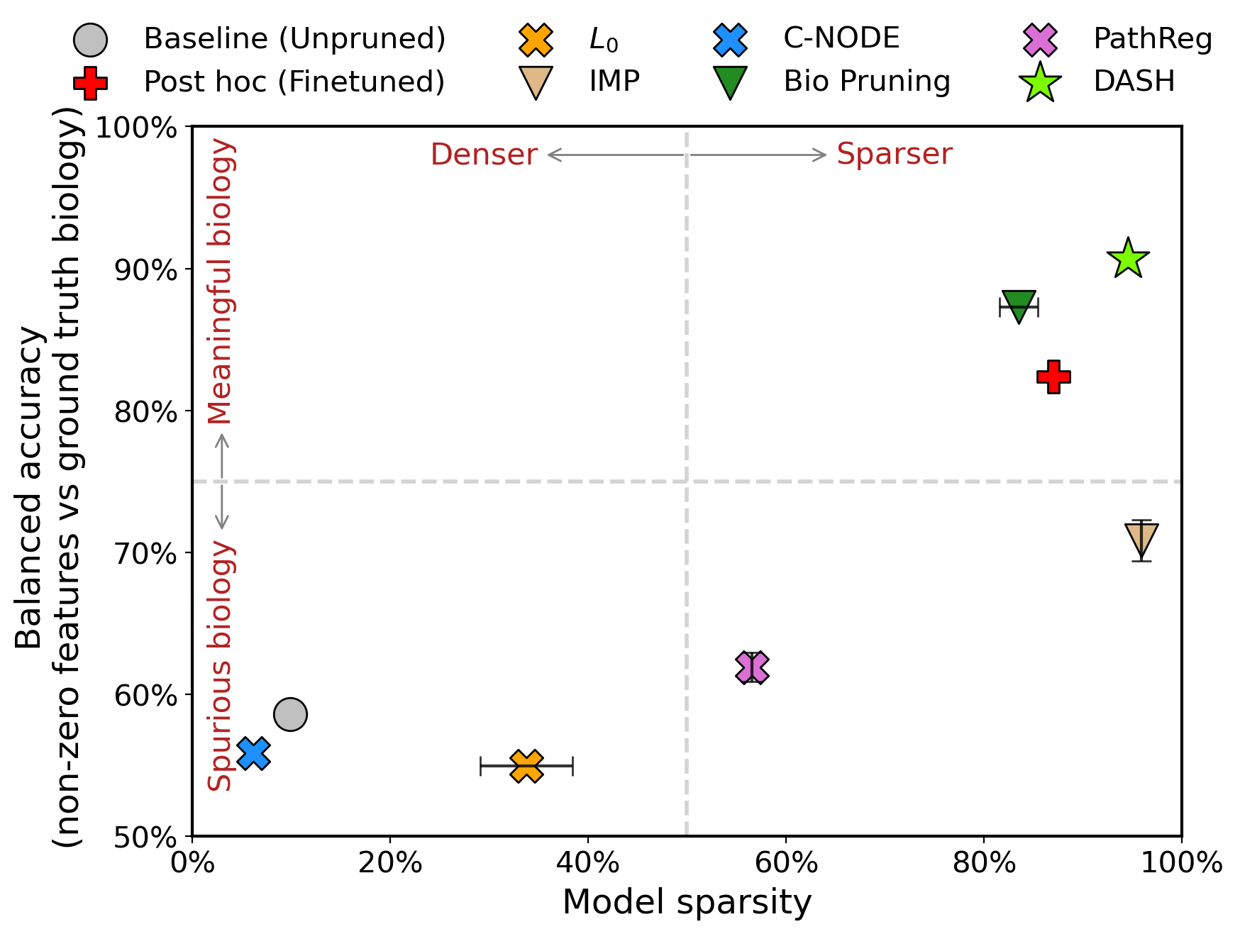
Figure 1: SIM350 data with 5% noise. We visualize performance of pruning strategies in comparison to original PHOENIX (baseline) in terms of achieved sparsity (x-axis) and balanced accuracy (y-axis) of the recovered gene regulatory network against the ground truth. Error bars are omitted when error is smaller than depicted symbol. Ideal models are in the top right quadrant; they recover the true, inherently sparse biological relationships.

While the aforementioned sparsification strategies have shown to perform in various settings, the resulting models are often either not really sparse or do not reflect meaningful insights, as we will also see in the later experiments. We hypothesize that this is due to the difficulty of identifying a good sparse network and suggest to ground the model search (or training) with existing domain-specific knowledge.

In the following, we introduce DASH (Domain-Aware Sparsity Heuristic), an iterative pruning-based approach that accounts for prior knowledge by scoring parameters in terms of their alignment with this prior. Furthermore, DASH contains a tuning parameter $\lambda$ to combine the data-informed weight matrices with prior-knowledge-informed effect matrices, which in practice can easily be found by cross validation. We begin with the simple case of a fully connected NN with $L=1$ layer.

3.1 DASH for $L=1$

For a single layer NN ($n$ inputs, $o$ outputs) with weights $\boldsymbol{W}\in\mathbb{R}^{o\times n}$, we compute corresponding non-negative pruning scores $\boldsymbol{\Omega}\in\mathbb{R}^{o\times n}$ by leveraging matrix $\boldsymbol{P}\in\mathbb{R}^{o\times n}$ encoding expertise/experiment driven putative effect sizes between the inputs and outputs. Such domain knowledge is common in areas such as genomics, where for example prior experimental evidence exists regarding the binding of $n$ transcription factors on $o$ target genes.

Alternating between training and pruning akin to Iterative Magnitude Pruning (Frankle & Carbin, 2018), we set the following pruning score during a pruning phase:

$$\boldsymbol{\Omega^{(t)}}:=(1-\lambda)\widetilde{|\boldsymbol{W^{(t)}}|}+\lambda|\boldsymbol{P}|,$$

where $\widetilde{|\boldsymbol{W^{(t)}}|}$ represents the appropriately normalized matrix (see Appendix B.2) of absolute weights as learned up to epoch $t$, and $\lambda\in[0,1]$ is a tuning parameter allowing the pruning to prioritize between the data and the prior information. We then prune the parameters in $\boldsymbol{W^{(t)}}$ corresponding to the lowest absolute $p_{t}\%$ of entries in $\boldsymbol{\Omega^{(t)}}$, where $p_{t}$ is the desired sparsity level at time $t$ given by a schedule.

3.2 DASH for $L=2$

For two-layered NNs with weights $\boldsymbol{W_{1}}\in\mathbb{R}^{m\times n},\boldsymbol{W_{2}}\in\mathbb{R}^{o\times m}$, prior knowledge might be available in different forms. As before, we might have access to putative prior effect sizes between the $n$ inputs and $o$ outputs $\boldsymbol{P}\in\mathbb{R}^{o\times n}$. Additionally, one might also have access to $\boldsymbol{C}\in\mathbb{R}^{n\times n}$ which encodes prior knowledge of how the $n$ inputs co-vary with each other in order to conjunctively act on the outputs. In genomics for example this would correspond to knowledge about interactions between transcription factors acting in a complex, which has also been employed to guide static gene regulatory network inference (Weighill et al., 2021).

Given that $\boldsymbol{W_{1}^{(t)}}$ represents how the $n$ inputs are encoded by $m$ neurons, we surmise that the inner product $\boldsymbol{{\Omega^{(t)}_{1}}^{\intercal}\Omega_{1}^{(t)}}\in\mathbb{R}^{n\times n}$ should approximately align with the prior knowledge $\boldsymbol{C}$. This motivates

$$\boldsymbol{\Omega_{1}^{(t)}}:=(1-\lambda_{1})\widetilde{|\boldsymbol{W_{1}^{(t)}}|}+\lambda_{1}\Big{|}\texttt{PInv}_{L}\Big{(}\boldsymbol{\Omega^{(t-1)}_{1}}^{\intercal}\Big{)}\cdot\boldsymbol{C}\Big{|},$$

where $\texttt{PInv}_{L}(X)$ and $\texttt{PInv}_{R}(X)$ represent the left and right pseudoinverses of $X$, s.t. $\texttt{PInv}_{L}(X)=(X^{\intercal}X)^{-1}X^{\intercal}$ and $\texttt{PInv}_{R}(X)=X^{\intercal}(XX^{\intercal})^{-1}$, and $\texttt{PInv}_{L}\Big{(}\boldsymbol{\Omega^{(t-1)}_{1}}^{\intercal}\Big{)}\cdot\boldsymbol{C}$ encourages $\boldsymbol{{\Omega^{(t)}_{1}}^{\intercal}\Omega_{1}^{(t)}}$ to iteratively align with $\boldsymbol{C}$ as $t$ increases (i.e. as training progresses). With $\boldsymbol{\Omega^{(t)}_{1}}$ fixed, we can update scores $\boldsymbol{\Omega^{(t)}_{2}}$ of the second layer parameters $\boldsymbol{W_{2}^{(t)}}$. Since the product $\boldsymbol{W_{2}^{(t)}\cdot W_{1}^{(t)}}\in\mathbb{R}^{o\times n}$ represents the overall flow of information from inputs to outputs at epoch $t$, we surmise that $(\boldsymbol{\Omega^{(t)}_{2}\Omega^{(t)}_{1}})\in\mathbb{R}^{o\times n}$ should reflect $\boldsymbol{P}$. We thus get

$$\boldsymbol{\Omega_{2}^{(t)}}:=(1-\lambda_{2})\widetilde{|\boldsymbol{W_{2}^{(t)}}|}+\lambda_{2}\Big{|}\boldsymbol{P}\cdot\texttt{PInv}_{R}\Big{(}\boldsymbol{\Omega^{(t)}_{1}}\Big{)}\Big{|}.$$

3.3 DASH for $L>2$

For many interpretability-centric tasks, including our case study, small architectures of $L=2$ are common, as domain experts are interested in understanding the exact flow of information through the network. Furthermore, we know that two-layer neural networks exhibit universal approximation given in the seminal result by Cybenko (1989). Appreciating also deep architectures, we however hypothesize that the technique of computing pruning scores by fixing those of preceding layers can easily be extended to a larger number $L$ of fully connected layers. We elaborate a potential derivation in App. B.6.

3.4 Flexibility and runtime

While the $\lambda_{l}$ can be tuned using cross-validation (see Appendix B.4), we also note that it allows for flexibly encoding different pruning philosophies. Specifically when $\lambda_{l}=0~{}\forall l$, DASH simply corresponds to IMP. Interestingly when $\lambda_{l}=1~{}\forall l$ (which we henceforth term “Bio pruning”), DASH represents fully prior-based sparsification. We subsequently include this baseline as BioPruning in our synthetic experiments, to understand the benefit of tuning $\lambda_{l}$ correctly.

It is noteworthy that unlike other methods (e.g. $L_{0}$) DASH does not prolong the runtime of training, as it only incurs a constant matrix multiplication overhead in pruning epochs.

4 Sparse gene regulatory dynamics

Here, we show that pruning aligned with prior information – in this case biological knowledge – improves interpretability as well as inferred data-specific knowledge. We picked the task of inferring gene regulatory dynamics, as it is important for foundational research of human biology but also clinical practice, as generated insights can be transferred to therapy design. Interpretability of such models is, hence, key. The most recent developments in modeling gene regulatory systems allow to model actual dynamics, but require complex models, such as NeuralODEs, that hinder interpretability.

While state-of-the-art results are now achieved with shallow architectures (Hossain et al., 2023) that are more tractable than deep, heavily over-parametrized networks, these models still encode information across many thousands of weights and we show experimentally that such information does not reflect true biology well. In fact, true gene regulatory networks and hence their underlying dynamics are inherently sparse (Busiello et al., 2017). This sparsity should be properly reflected by neural dynamics models. This line of NeuralODEs will serve as our base model for applying sparsification strategies.

In a nutshell, given a time series gene expression sample for $n$ genes, PHOENIX uses NeuralODEs to construct the predicted trajectory between gene expression $\boldsymbol{g}(t)\in\mathbb{R}^{n}$ at time $t=t_{i}$ to any future expression $\widehat{\boldsymbol{g}}(t_{i+1})$, by implicitly modelling the RNA velocity ($d\boldsymbol{g}/dt$). PHOENIX utilizes biokinetics-inspired activation functions to separately model additive and multiplicative coregulatory effects. The trained model encodes the ODEs governing the dynamics of gene expression, which can be directly extracted for biological insights. In the following, we provide an outline of the PHOENIX architecture and refer to Appendix C for further details of the method, before we demonstrate how DASH can be applied to this architecture.

4.1 Neural ordinary differential equations

NeuralODEs (Chen et al., 2018) learn dynamical systems by parameterizing the underlying derivatives with neural networks: $\frac{d\boldsymbol{g}(t)}{dt}=f(\boldsymbol{g}(t),t)\approx\text{NN}_{\Theta}(\boldsymbol{g}(t),t).$ Given an initial condition $\boldsymbol{g}(t_{0})$, the output $\boldsymbol{g}(t_{i})$ at any given time-point $t_{i}$ can now be approximated using a numerical ODE solver of adaptive step size:

$$\widehat{\boldsymbol{g}(t_{1})}=\boldsymbol{g}(t_{0})+\int_{t_{0}}^{t_{1}}\text{NN}_{\Theta}(\boldsymbol{g}(t),t)~{}dt.$$

A loss function $L\Big{(}\boldsymbol{g}(t_{1})~{}\boldsymbol{;}~{}\boldsymbol{g}(t_{0})+\int_{t_{0}}^{t_{1}}\text{NN}_{\Theta}(\boldsymbol{g}(t),t)~{}dt\Big{)}$ is then optimized for $\Theta$ via back propagation, using the adjoint sensitivity method (Cao et al., 2003) to carry the backpropagation through the integration steps of the ODESolver.

4.2 PHOENIX - overview

PHOENIX models gene expression dynamics using NeuralODEs. Notably, for an expression vector of $n$ genes, PHOENIX models both additive and multiplicative regulatory effects using two parallel linear layers with $m$ neurons each: $\text{NN}_{sums}$ (with weights $\boldsymbol{W_{\Sigma}}\in\mathbb{R}^{m\times n}$, and biases $\boldsymbol{b_{\Sigma}}\in\mathbb{R}^{m}$) and $\text{NN}_{prods}$ ($\boldsymbol{W_{\Pi}}\in\mathbb{R}^{m\times n}$, $\boldsymbol{b_{\Pi}}\in\mathbb{R}^{m}$). Here, $\text{NN}_{sums}$ and $\text{NN}_{prods}$ are equipped with activation functions that model the Hill equation

$$\phi_{\Sigma}(x)=\frac{x-0.5}{1+\mid x-0.5\mid}~{}~{}\text{and}~{}~{}\phi_{\Pi}(x)=\log\Big{(}\phi_{\Sigma}(x)+1\Big{)}.$$

The Hill equation is a classical formula in biochemistry that models molecular binding in dependence of concentration. This results in outputs of the two parallel layers

$$\boldsymbol{c_{\Sigma}}(\boldsymbol{g}(t)) =\boldsymbol{W_{\Sigma}}\phi_{\Sigma}(\boldsymbol{g}(t))+\boldsymbol{b_{\Sigma}}~{}~{}\text{and}$$

$$\boldsymbol{c_{\Pi}}(\boldsymbol{g}(t)) =\exp\circ(\boldsymbol{W_{\Pi}}\phi_{\Pi}(\boldsymbol{g}(t))+\boldsymbol{b_{\Pi}}).$$

As shown above, $\phi_{\Pi}(x)$ yields the output of $\text{NN}_{prods}$ in the log space and is subsequently exponentiated in $\boldsymbol{c_{\Pi}}$ to represent multiplicative effects in the linear space. The outputs $\boldsymbol{c_{\Sigma}}(\boldsymbol{g}(t))$ and $\boldsymbol{c_{\Pi}}(\boldsymbol{g}(t))$ are then separately fed into two more parallel linear layers $\text{NN}_{\Sigma combine}$ (with weights $\boldsymbol{U}_{\Sigma}\in\mathbb{R}^{n\times m}$) and $\text{NN}_{\Pi combine}$ ($\boldsymbol{U}_{\Pi}\in\mathbb{R}^{n\times m}$), respectively. The outputs of $\text{NN}_{\Sigma combine}$ and $\text{NN}_{\Pi combine}$ are summed to obtain

$$\boldsymbol{c_{\cup}}(\boldsymbol{g}(t)) =\boldsymbol{U}_{\Sigma}\boldsymbol{c_{\Sigma}}(\boldsymbol{g}(t))+\boldsymbol{U}_{\Pi}\boldsymbol{c_{\Pi}}(\boldsymbol{g}(t)).$$

Finally, PHOENIX includes gene-specific multipliers $\boldsymbol{\upsilon}\in\mathbb{R}^{n}$ for modelling steady states of genes that do not exhibit any temporal variation $\big{(}\frac{dg_{i}(t)}{dt}=0,\forall t\big{)}$. Accordingly, the output for each gene $i$ in $\boldsymbol{c_{\cup}}(\boldsymbol{g}(t))$ is multiplied with $\text{ReLU}(\upsilon_{i})$ in the final estimate for the local derivative

$$\text{NN}_{\Theta}(\boldsymbol{g}(t),t)=\text{ReLU}(\boldsymbol{\upsilon})\odot\Big{[}\boldsymbol{c_{\cup}}(\boldsymbol{g}(t))-\boldsymbol{g}(t)\Big{]}.$$

Although PHOENIX achieves some sparsity in its weight matrices ($\boldsymbol{W_{\Sigma}},\boldsymbol{W_{\Pi}},\boldsymbol{U_{\Sigma}},\boldsymbol{U_{\Pi}}$), the achieved sparsity level is, however, at most $12\%$ (see Figure 1, and Tables 1, 4, 5).

4.3 Subjecting PHOENIX to DASH pruning

With its simple yet powerful architecture, PHOENIX provides an ideal base setting for applying and testing the merits of the discussed neural network sparsification strategies (Section 2), including DASH. We discuss the DASH implementation here and provide implementation details for other sparsification strategies in Appendix B.9.

For DASH, we follow the steps of the $L=2$ case in Section 3.2, applied separately on each parallel member of the first $\{\boldsymbol{W_{\Sigma}},\boldsymbol{W_{\Pi}}\}$ and second $\{\boldsymbol{U_{\Sigma}},\boldsymbol{U_{\Pi}}\}$ layers. For the first layer, we leverage prior knowledge of transcription factor coregulation (often available in the form of protein-protein interaction matrices) to formulate $\boldsymbol{C}\in\mathbb{R}^{n\times n}$. This is then used to calculate pruning scores $\boldsymbol{\Omega_{\Sigma}},\boldsymbol{\Omega_{\Pi}}$ for $\boldsymbol{W_{\Sigma}},\boldsymbol{W_{\Pi}}$. Similarly, for $\boldsymbol{U_{\Sigma}},\boldsymbol{U_{\Pi}}$ in the second layer, we utilize $\boldsymbol{P}\in\mathbb{R}^{n\times n}$ which are easily obtainable motif map matrices encoding prior knowledge of transcription factor binding sites around genes to calculate pruning scores $\boldsymbol{\Psi_{\Sigma}},\boldsymbol{\Psi_{\Pi}}$. We illustrate this in Algorithm 1.

Algorithm 1 Computing $\boldsymbol{\Omega_{\Sigma}^{(t)}},\boldsymbol{\Omega_{\Pi}^{(t)}},\boldsymbol{\Psi_{\Sigma}^{(t)}},\boldsymbol{\Psi_{\Pi}^{(t)}}$

  Inputs: weights $\boldsymbol{W_{\Sigma}^{(t)}},\boldsymbol{W_{\Pi}^{(t)}}$,$\boldsymbol{U_{\Sigma}^{(t)}},\boldsymbol{U_{\Pi}^{(t)}}$; priors $\boldsymbol{C},\boldsymbol{P}$; epoch $t$; previous scores $\boldsymbol{\Omega_{\Sigma}^{(t-1)}},\boldsymbol{\Omega_{\Pi}^{(t-1)}}$; tuning $\lambda_{1},\lambda_{2}$

  Normalize $\boldsymbol{W_{\Sigma}^{(t)}}$ to get $|\widetilde{\boldsymbol{W_{\Sigma}^{(t)}}}|$ (see Appendix B.2)

  Similarly obtain $|\widetilde{\boldsymbol{W_{\Pi}^{(t)}}}|$, $|\widetilde{\boldsymbol{U_{\Sigma}^{(t)}}}|$, and $|\widetilde{\boldsymbol{U_{\Pi}^{(t)}}}|$

  if $t=0$ then

     Initialize $\boldsymbol{\Omega_{\Sigma}^{(t)}}:=\boldsymbol{1}$, and $\boldsymbol{\Omega_{\Pi}^{(t)}}:=\boldsymbol{1}$

  else

     $\boldsymbol{\Omega_{\Sigma}^{(t)}}:=(1-\lambda_{1})\widetilde{|\boldsymbol{W_{\Sigma}^{(t)}}|}+\lambda_{1}\Big{|}\texttt{PInv}_{L}\Big{(}\boldsymbol{\Omega_{\Sigma}^{(t-1)}}^{\intercal}\Big{)}\cdot\boldsymbol{C}\Big{|}$

     $\boldsymbol{\Omega_{\Pi}^{(t)}}:=(1-\lambda_{1})\widetilde{|\boldsymbol{W_{\Pi}^{(t)}}|}+\lambda_{1}\Big{|}\texttt{PInv}_{L}\Big{(}\boldsymbol{\Omega_{\Pi}^{(t-1)}}^{\intercal}\Big{)}\cdot\boldsymbol{C}\Big{|}$

  end if

  $\boldsymbol{\Psi_{\Sigma}^{(t)}}:=(1-\lambda_{2})\widetilde{|\boldsymbol{U_{\Sigma}^{(t)}}|}+\lambda_{2}\Big{|}\boldsymbol{P}\cdot\texttt{PInv}_{R}\Big{(}\boldsymbol{\Omega_{\Sigma}^{(t)}}\Big{)}\Big{|}$

  $\boldsymbol{\Psi_{\Pi}^{(t)}}:=(1-\lambda_{2})\widetilde{|\boldsymbol{U_{\Pi}^{(t)}}|}+\lambda_{2}\Big{|}\boldsymbol{P}\cdot\texttt{PInv}_{R}\Big{(}\boldsymbol{\Omega_{\Pi}^{(t)}}\Big{)}\Big{|}$

5 Experiments

Table 1: Results on SIM350 data with 5% noise. We give model sparsity, balanced accuracy with respect to edges in the ground truth gene regulatory network, mean squared error of predicted gene regulatory dynamics, and number of epochs as proxy of runtime.

Pruning strategy		Sparsity(%)	Bal. Acc.(%)	Test MSE ($10^{-3}$)	Epochs
None/Baseline    (Hossain et al., 2023)		$9.9\pm 0.4$	$58.6\pm 0.7$	$2.5\pm 0.2$	$160\pm 7$
Post hoc + Fine tuning		$87.0\pm 0.01$	$82.4\pm 0.2$	$\bf{2.3\pm 0.3}$	$1721\pm 50$
Penalty (implicit)	$L_{0}$ (Louizos et al., 2017)	$33.8\pm 4.7$	$55.0\pm 0.5$	$8.5\pm 1.0$	$134\pm 37$
	C-NODE (Aliee et al., 2021)	$6.2\pm 0.5$	$55.9\pm 0.1$	$2.8\pm 0.6$	$214\pm 4$
	PathReg (Aliee et al., 2022)	$56.5\pm 1.5$	$61.9\pm 1.0$	$8.0\pm 1.8$	$200\pm 29$
Iterative (explicit)	IMP (Frankle & Carbin, 2018)	$\bf{96.0\pm 0.01}$	$70.9\pm 1.5$	$3.6\pm 0.6$	$220\pm 3$
	Bio Pruning (see section 3.4)	$83.5\pm 1.9$	$87.3\pm 0.8$	$2.6\pm 0.9$	$79\pm 2$
	DASH (Ours)	$94.6\pm 1.2$	$\bf{90.7\pm 0.4}$	$2.4\pm 1.2$	$192\pm 24$

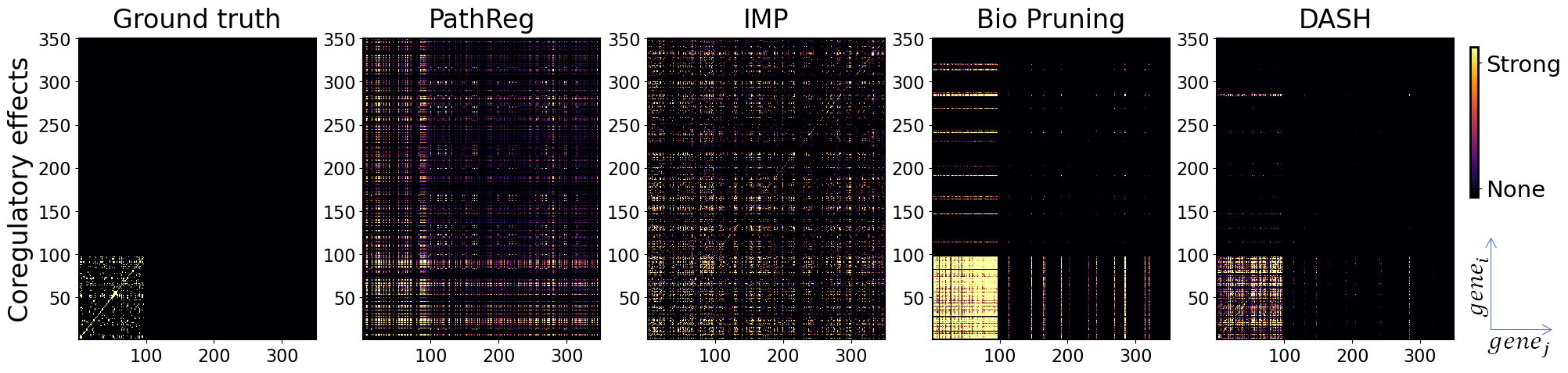
Figure 2: Estimated coregulatory effects in SIM350 data. We plot the estimated coregulation of gene $g_{j}$ (x-axis) and gene $g_{i}$ (y-axis). All results are reported on SIM350 with 5% of noise. See Appendix A.2 for results on additional noise settings and number of genes.

For evaluation we consider synthetic data with known ground truth regulatory relationships, as well as real world data of breast cancer gene expression with measurements of transcription factor binding that serve as a gold standard reference for the inferred gene regulatory network (Desmedt et al., 2007). In an exploratory analysis, we further consider real world single-cell gene expression data of blood hematopoiesis (Aliee et al., 2022). To compare pruning strategies, we consider the PHOENIX model as a basis, which is the state-of-the-art NeuralODE for estimating gene regulatory dynamics (Hossain et al., 2023).

As baselines we consider the PHOENIX model without additional pruning, already achieving some sparsity, post-hoc magnitude pruning of weights with additional finetuning of the pruned weights, and Bio Pruning (introduced in Section 3.4) . From the literature, we consider Iterative Magnitude Pruning (IMP) (Frankle & Carbin, 2018), which has been shown to be successful for Neural ODEs (Liebenwein et al., 2021), $L_{0}$-regularized pruning (Louizos et al., 2017), as well as C-NODE (Aliee et al., 2021) and PathReg (Aliee et al., 2022), which have been recently proposed for the inference of sparse gene-regulatory relationships.

5.1 Simulated gene regulatory systems

We simulate gene expression time-series data from a fixed dynamical system, the ground truth was thus known (see Appendix B.1). In short, we adapt SimulatorGRN (Bhuva et al., 2019) to generate noisy time-series expression data from two synthetic gene regulatory systems (SIM350 and SIM690, consisting of 350 and 690 genes, respectively). We split trajectories into training (88%), validation (6% for tuning $\lambda$), and testing (6%).We evaluate all methods in terms of achieved model sparsity and MSE of predicted gene expression values on the test set (see Appendix B.2, B.4). We also investigate biological alignment by calculating balanced accuracy of GRNs extracted from PHOENIX (see Appendix C.2, B.5),

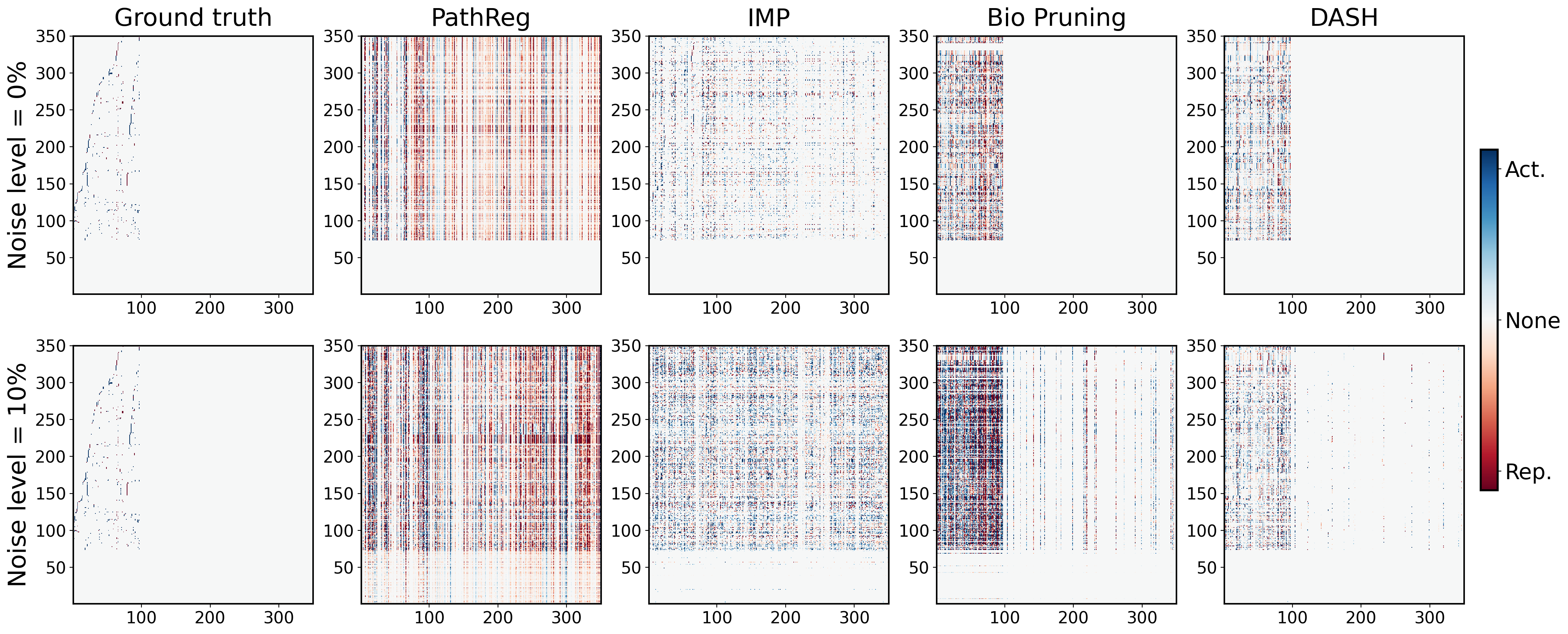
Figure 5: Estimated effect of gene $g_{j}$ (x-axis) on the dynamics of gene $g_{i}$ (y-axis) in SIM350 at 0% and 10% noise, across different pruning strategies.

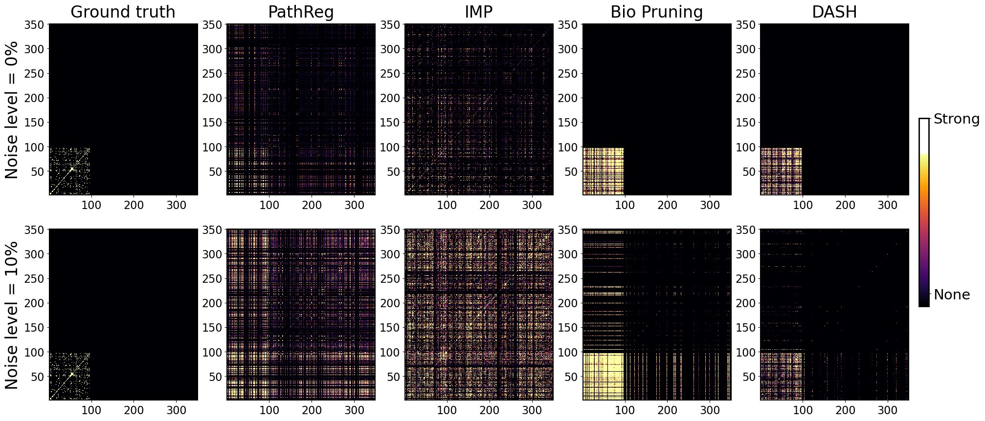
Figure 6: Estimated coregulation of $g_{i}$ and $g_{j}$ in SIM350 at 0%, 10% noise, across different pruning strategies.

Sparsity corresponds to meaningfulness. We here report the results for the data of 350 genes and 5% noise, noting that results are consistent across different noise levels (see App. Tables 4, 5 and App. Figures 5, 6) and with more number of genes (see App. Table 7). A general trend across all experiments that aligns with our initial motivation is that dense models (sparsity $<$ 50%) have a significantly worse reconstruction of the underlying biology – the ground truth GRN – than sparse models (sparsity $>$ 80%) (see Figure 1). Furthermore, we see that DASH retrieves not only among the sparsest networks, but also reflects the underlying GRN best across all methods, outperforming comparably sparse IMP by about 20 percentage points accuracy in different settings. Due to the prior-informed structured pruning, it is able to occupy the sweet spot of highly sparse at the same time biologically meaningful models (Figure 1 top right).

DASH is sparse and performant. Consistent with the literature, PathReg outperforms both $L_{0}$ as well as C-NODE in terms of sparsity (Aliee et al., 2022), here we additionally find evidence that it also delivers more biologically meaningful results. Yet, IMP as well as prior-informed pruning approaches outperform PathReg by a margin. The MSE of predicted gene expression of DASH is among the best, within one standard error of the best overall method. The only better approach is a combination of posthoc magnitude pruning of PHOENIX combined with additional finetuning, which is, however, impractical as it requires to train and prune PHOENIX multiple times along a grid of sparsity levels (see Appendix B.9.2), evident in the number of required epochs (Table 1, Appendix Tables 4, 5, 7). DASH, in contrast, automatically finds good sparsity for PHOENIX in a time comparable to other competitors such as IMP.

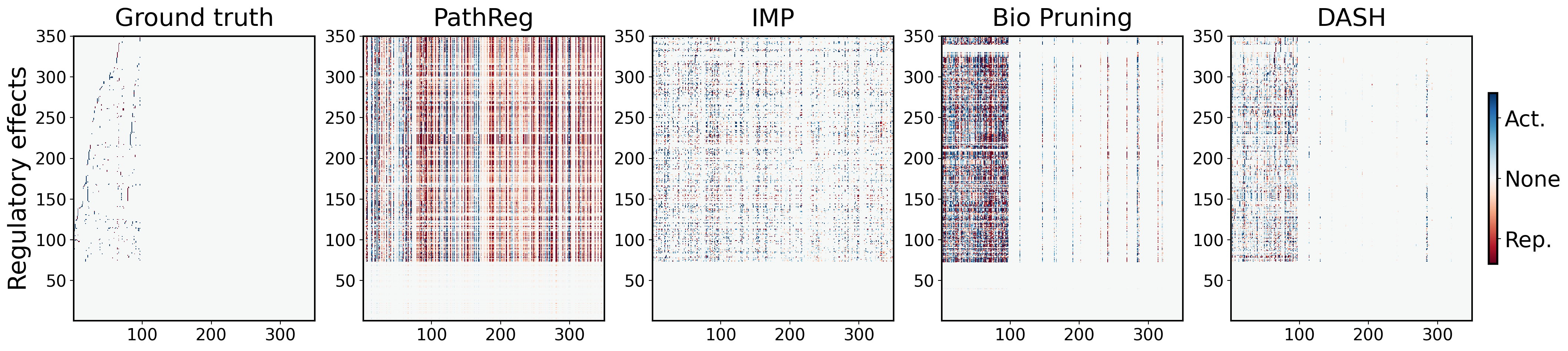
Figure 4: Estimated effect of gene $g_{j}$ (x-axis) on the dynamics of gene $g_{i}$ (y-axis) in SIM350 at 5% noise, across different pruning strategies.

DASH recovers causal directions. Visualizing the estimated against ground truth regulatory effects (i.e., functional relationships between variables), we observe that DASH captures the effects much better than competitors (see App Figure 4). Both PathReg as well as IMP introduce a lot of regulatory effects that should not exist (i.e., they are in the anti-causal direction), whereas prior-informed pruning (BioPruning and DASH) capture the main regulatory effects in a correct causal direction. While not yet perfect, DASH provides a sparse estimation of regulatory effects that resembles the ground truth relationships. Similarly, the estimated co-regulation (i.e., correlation between effects of causal variables) is best captured by DASH (see Figure 2).

5.2 Pseudotime-ordered breast cancer samples

To investigate the performance of DASH on challenging real data, we consider gene expression measurements from a cross-sectional breast cancer study (Desmedt et al., 2007). This data of 198 breast cancer patients with measurements for 22000 genes has been preprocessed and ordered in pseudotime by Sun et al. (2021), which we use as basis for our experiments (see Appendix B.7).

DASH recovers gene regulatory relationships. Consistent with our results on the synthetic data, we observe that PathReg outperforms both C-NODE as well as $L_{0}$ among the regularizer-based sparsification strategy in terms of achieved sparsity. Yet, the sparsity levels are comparitively low with only 15% sparsity compared to the original model. DASH achieves a high model sparsity of more than 90% while recovering the underlying gene regulatory network with 95% accuracy (see Table 2). As before, only IMP achieves a higher sparsity, however, it does not reflect true biology with an essentially random edge reconstruction compared to the reference GRN. In fact, all competitors show this random reconstruction performance on this challenging real data of a difficult heterogeneous cancer.

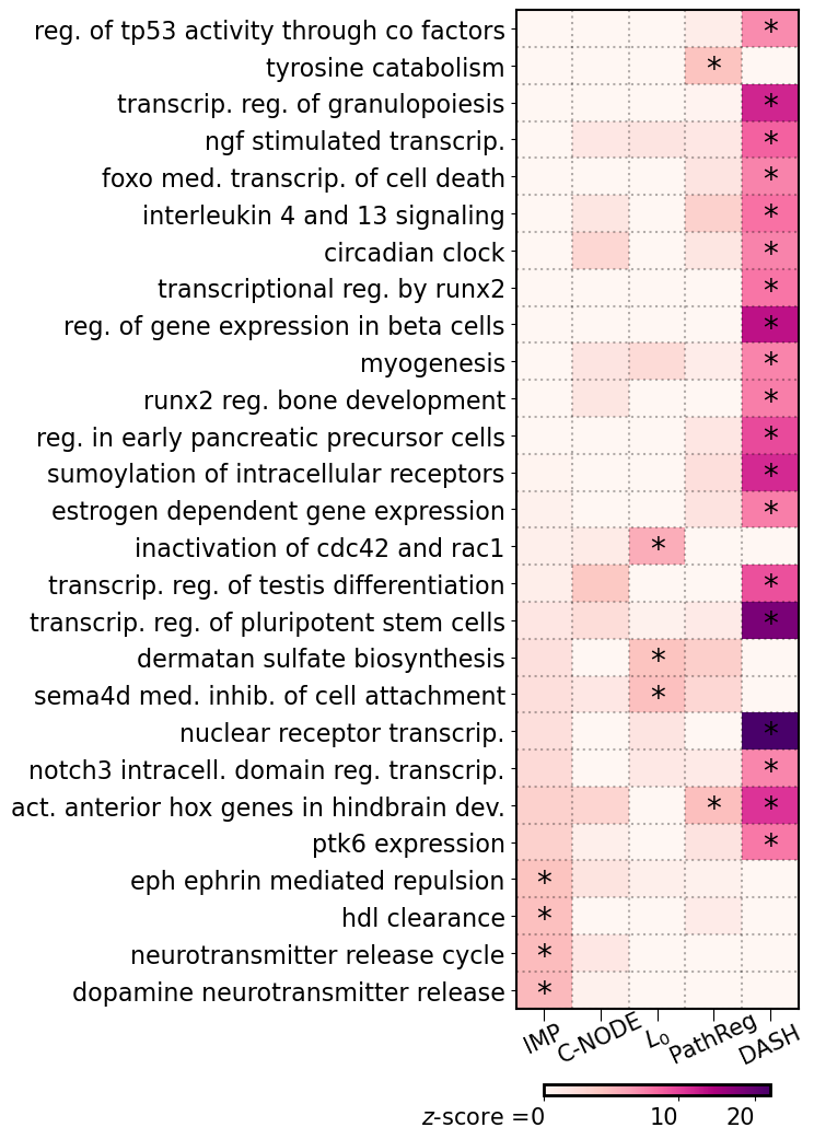
Figure 7: BRCA pathway analysis. We visualize the top-20 significant pathways for each method. For each method (x-axis) we show the pathway z-score and indicate significant results after FWER correction (Bonferroni, p-value cutoff at $.05$) with *. All competitors find overall very few significant pathways and hence very few insights into biology.

DASH finds meaningful biology. To better understand whether the inferred gene regulatory dynamics align with meaningful biology, we perform a permutation-based pathway analysis (see Appendix B.8). Here, the genes that show the highest impact on the dynamics within the derived model are mapped to higher level biological pathways and it is tested whether certain pathways are particularly enriched for genes found important in the model. Visualizing the top-20 most significant pathways of each method (App Fig 7), we observe that in contrast to DASH, the existing pruning approaches show only very few significant pathways, which reflects the previous results comparing to the inferred GRN to the reference GRN available through gold standard experiments for this data set. Moreover, disease-relevant pathways such as TP53 activity or FOXO mediated cell death, both of which are highly relevant in cancer (Marvalim et al., 2023; Jiramongkol & Lam, 2020), are only visible in DASH. This provides evidence that pruning informed by a biological prior recovers biological signals that are relevant in the disease and which can not be picked up otherwise. Such pathway analysis are a standard approach for domain experts to distill information for example for therapeutic designs and, hence, good biological signals are essential.

5.3 Cell differentiation in human bone marrow

Lastly, we investigate the performance of DASH in an exploratory setting with over $12,000$ samples of single cell data of human bone marrow ordered in pseudotime (Aliee et al., 2022). Here, we are interested in better understanding the gene regulatory dynamics of blood cell differentiation, the process of hematopoietic stem cells specializing into cells taking over roles such as immune response (e.g., B- and T-cells). This process is called hematopoiesis. As described in Appendix B.7, we follow the steps of Aliee et al. (2022) to first split samples (i.e., cells) into the three different lineages (paths of differentiation), and train separate models for each of these splits. In the following, we will focus on the analysis of the Erythroid lineage and provide results for the other lineages (Monocyte and B-cell) in Appendix A.4. As previous results showed that PathReg outperforms C-NODE and $L_{0}$ on this particular data (Aliee et al., 2022), we focus on the comparison of DASH with IMP and PathReg.

DASH consistently identifies sparse models. As before, DASH achieves very high sparsity of more than 95%, the most sparse network among all competitors (Tab. 3). IMP shows similarly strong sparsification as DASH. PathReg, however, only achieves an order of magnitude less sparsity of around 14%. In terms of performance of regulatory dynamics prediction, all methods achieve similar MSE on a hold-out test set, meaning that even though much sparser, both DASH and IMP predict equally well as an order of magnitude more dense network.

DASH provides biological insights. As we do not have ground truth or reference information about the underlying gene regulatory system, we resort to quantitatively evaluating the connectedness of the inferred gene regulatory network in terms of the average out-degree. DASH shows the lowest out-degree, less than half of what IMP recovers. PathReg – not unexpectedly given the sparsity difference – shows an order of magnitude larger average out-degree in the inferred GRN. We would expect sparser networks to be better align with biology (Busiello et al., 2017). To confirm, we carry out a pathway analysis similar to our breast cancer study. As before, only DASH seems to find significant enrichment in biologically relevant pathways (see Fig. 3). Both IMP as well as PathReg both find only one significant pathway after multiple test correction, and its biological relation to hematopoiesis is not immediately clear. DASH on the other hand finds pathways that can immediately be linked to hematopoiesis, such as heme signaling or RUNX1 regulates differentiation of hematopoietic stem cells. We, hence, suspect that the biological system inferred by DASH reflects meaningful biology from the domain of the data.

Table 2: Results on breast cancer. Balanced accuracy is based on reference gold standard experiments available for this data.

Strategy	Sparsity	Bal. Acc.	MSE ($10^{-5}$)
None	0.03%	49.99%	7.78
$L_{0}$	10.38%	50.15%	7.90
C-NODE	0.01%	50.01%	8.06
PathReg	14.92%	50.24%	7.92
IMP	$\bf{95.70\%}$	49.70%	7.76
DASH	92.71%	$\bf{95.69\%}$	7.76

Table 3: Results on Hematopoesis data for the Erythroid lineage.

Strategy	Sparsity	OutDeg	Test MSE ($10^{-4}$)
PathReg	13.94%	522	2.12
IMP	94.44%	123	2.12
DASH	95.95%	54	2.12

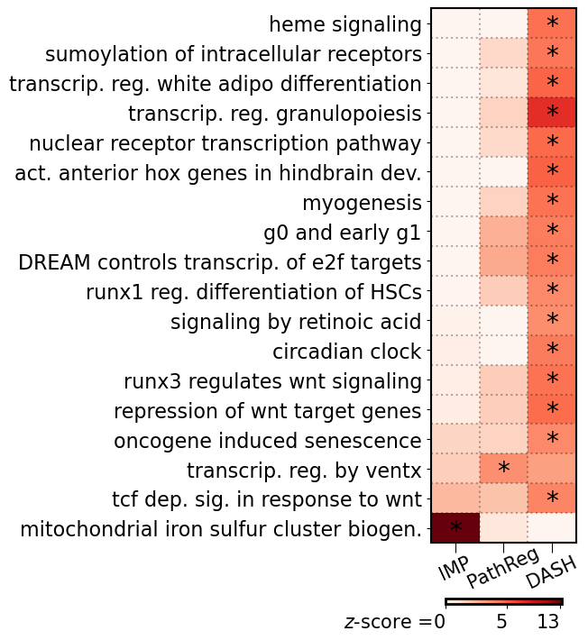
Figure 3: Hematopoesis pathway analysis. We visualize the top-20 significantly enriched pathways on the Erythroid lineage. For each method (x-axis) we show the pathway z-score and indicate significant results after FWER correction (Bonferroni, p-value cutoff at $.05$) with *.

6 Discussion & Conclusion

We considered the problem of identifying sparse neural networks in the context of interpretability. In domains such as biology and contexts when the true underlying systems are sparse, interpretability is key for experts, rendering the use of the common over-parametrized and complex neural network architectures difficult. Recent advances in neural network pruning, such as those around the Lottery Ticket Hypothesis (Frankle & Carbin, 2018), promise sparse and well-performing models, yet, hardness results prove finding optimally sparse models to be challenging (Malach et al., 2020), which is also reflected by recent benchmarking results (Fischer & Burkholz, 2022). Our experiments confirm that general pruning strategies suffer from identifiability issues and propose to guide pruning by domain knowledge.

In case studies on gene regulatory dynamic inference based on synthetic as well as real world data, we have shown that our method, DASH, in contrast to the state of the art is able to recover models that are both very sparse and at the same time biologically meaningful. On synthetic data, DASH better recovers the underlying ground truth regulatory network, and better recapitulates causal directions of regulation. On real data, DASH better alignes with gold-standard experimental evidence of regulatory interactions. In analysis mapping to biological pathways, which is commonly used to inform domain experts to generate new insights, DASH consistently finds biological information reflecting the biology of the specific data. Furthermore, DASH is computationally fast as it only incurs a small constant overhead of matrix multiplications during pruning, comparable to existing pruning approaches. It thus serves as a proof of concept that in critical domains, where interpretability is essential and domain knowledge exists, pruning can be heavily improved by alignment with prior knowledge.

While our guided pruning approach is in principle agnostic to the type of neural network and task, we here focused on a specific case study that we deemed important. In the future, it would be interesting to apply DASH to different cases and domains, including other biomedical tasks, but also to physics or material sciences, where interpretability is also key and domain knowledge exists in the form of physical constraints and models. Furthermore, an iterative procedure for a many-layered neural network (as outlined in the appendix) would be an interesting line of future work.

In summary, we make a case for pruning informed by domain knowledge and provide evidence that such approaches can massively improve sparsity along with domain specific interpretability.

Appendix A Supplementary results

A.1 Code availability

All code is available via GitHub: https://github.com/QuackenbushLab/DASH

A.2 Synthetic data

Table 4: Explainability results (measured as balanced accuracy) across sparsification strategies at 0% noise level for SIM350 (the synthetic system of 350 genes).

Pruning strategy		Sparsity (%)	Bal. Acc.(%)	Test MSE ($10^{-3}$)	Epochs
None/Baseline		11.3 $\pm$ 0.3	$60.3\pm 0.3$	$2.3\pm 0.4$	$206\pm 7$
Post hoc + Fine tuning		90.0 $\pm$ 0.01	$89.8\pm 0.3$	$2.6\pm 0.5$	$1788\pm 77$
Penalty (implicit)	$L_{0}$	34.7 $\pm$ 2.4	$61.3\pm 0.1$	$6.1\pm 1.8$	$119\pm 43$
	C-NODE	10.7 $\pm$ 0.2	$60.5\pm 0.1$	$\bf{1.9\pm 0.5}$	$213\pm 5$
	PathReg	59.7 $\pm$ 1.5	$64.2\pm 0.8$	$6.1\pm 2.3$	$213\pm 7$
Iterative (explicit)	IMP	$\bf{95.8\pm 0.3}$	$72.8\pm 0.7$	$2.9\pm 0.5$	$195\pm 16$
	Bio Pruning	83.5 $\pm$ 3.5	$88.0\pm 0.5$	$3.6\pm 0.8$	$94\pm 22$
	DASH	92.6 $\pm$ 1.2	$\bf{91.1\pm 1.2}$	$\bf{1.9\pm 0.6}$	$164\pm 22$

Table 5: Explainability results (measured as balanced accuracy) across sparsification strategies at 10% noise level for SIM350 (the synthetic system of 350 genes).

Pruning strategy		Sparsity(%)	Bal. Acc.(%)	Test MSE ($10^{-3}$)	Epochs
None/Baseline		$2.9\pm 0.5$	$51.3\pm 0.3$	$5.5\pm 1.9$	$211\pm 15$
Post hoc + Fine tuning		$\bf{92.0\pm 0.01}$	$83.8\pm 0.7$	$\bf{4.1\pm 1.8}$	$1813\pm 94$
Penalty (implicit)	$L_{0}$	$31.9\pm 1.6$	$50.2\pm 0.3$	$13.3\pm 1.8$	$156\pm 11$
	C-NODE	$7.2\pm 0.3$	$50.5\pm 0.3$	$36.6\pm 12.5$	$189\pm 11$
	PathReg	$47.8\pm 1.8$	$50.2\pm 1.2$	$12.7\pm 1.4$	$224\pm 8$
Iterative (explicit)	IMP	$89.9\pm 5.0$	$63.8\pm 3$	$5.1\pm 0.8$	$142\pm 13$
	Bio Pruning	$79.7\pm 1.3$	$85.2\pm 0.3$	$5.6\pm 0.3$	$67\pm 18$
	DASH	$90.8\pm 4.7$	$\bf{85.4\pm 4.2}$	$5.8\pm 1.3$	$154\pm 4$

Table 6: Interaction of pruning with domain-knowledge interaction term in PHOENIX across different noise levels.

Noise	Pruning strategy	PHOENIX regularizer	Sparsity(%)	Bal. Acc.(%)	Test MSE ($10^{-3}$)
0%	IMP	Excluded (default)	$\bf{95.8\pm 0.3}$	$72.8\pm 0.7$	$2.9\pm 0.5$
		Included	95.5 $\pm$ 0.5	$77.8\pm 1.3$	$4.0\pm 0.8$
	DASH	Excluded (default)	92.6 $\pm$ 1.2	$\bf{91.1\pm 1.2}$	$\bf{1.9\pm 0.6}$
		Included	89.1 $\pm$ 5.8	$86.8\pm 6.7$	$3.1\pm 1.3$
5%	IMP	Excluded (default)	$\bf{96.0\pm 0.01}$	$70.9\pm 1.5$	$3.6\pm 0.6$
		Included	$95.3\pm 0.3$	$75.8\pm 2.2$	$3.4\pm 1.7$
	DASH	Excluded (default)	$94.6\pm 1.2$	$\bf{90.7\pm 0.4}$	$2.4\pm 1.2$
		Included	$93.2\pm 0.7$	$90.6\pm 0.7$	$\bf{2.0\pm 1.0}$
10%	IMP	Excluded (default)	$89.9\pm 5.0$	$63.8\pm 3$	$\bf{5.1\pm 0.8}$
		Included	$88.4\pm 4.7$	$65.0\pm 5.9$	$5.8\pm 0.5$
	DASH	Excluded (default)	$\bf{90.8\pm 4.7}$	$\bf{85.4\pm 4.2}$	$5.8\pm 1.3$
		Included	$86.8\pm 5.7$	$82.0\pm 7.8$	$6.0\pm 2.3$

Table 7: Results across different number of genes $N_{g}$, either 350 or 690. Noise is 5%.

$N_{g}$	Pruning strategy		Sparsity(%)	Bal. Acc.(%)	Test MSE ($10^{-3}$)	Epochs
350	None/Baseline		$9.9\pm 0.4$	$58.6\pm 0.7$	$2.5\pm 0.2$	$160\pm 7$
	Post hoc + Fine tuning		$87.0\pm 0.01$	$82.4\pm 0.2$	$\mathbf{2.3\pm 0.3}$	$1621\pm 50$
	Penalty (implicit)	$L_{0}$	$33.8\pm 4.7$	$55.0\pm 0.5$	$8.5\pm 1.0$	$134\pm 37$
		C-NODE	$6.2\pm 0.5$	$55.9\pm 0.1$	$2.8\pm 0.6$	$214\pm 4$
		PathReg	$56.5\pm 1.5$	$61.9\pm 1.0$	$8.0\pm 1.8$	$200\pm 29$
	Iterative (explicit)	IMP	$\mathbf{96.0\pm 0.01}$	$70.9\pm 1.5$	$3.6\pm 0.6$	$220\pm 3$
		Bio Pruning	$83.5\pm 1.9$	$87.3\pm 0.8$	$2.6\pm 0.9$	$79\pm 2$
		DASH	$94.6\pm 1.2$	$\bf{90.7\pm 0.4}$	$2.4\pm 1.2$	$192\pm 24$
690	None/Baseline		$7.7\pm 0.1$	$56.7\pm 0.03$	$4.3\pm 0.3$	$166\pm 29$
	Post hoc + Fine tuning		$87.0\pm 0.01$	$75.9\pm 0.2$	$3.7\pm 0.2$	$1657\pm 106$
	Penalty (implicit)	$L_{0}$	$34.9\pm 1.1$	$53.0\pm 0.3$	$12.8\pm 3.1$	$100\pm 26$
		C-NODE	$4.3\pm 0.4$	$54.0\pm 0.2$	$24.4\pm 10.2$	$210\pm 2$
		PathReg	$57.7\pm 0.5$	$57.4\pm 0.2$	$35.3\pm 2.2$	$244\pm 17$
	Iterative (explicit)	IMP	$\mathbf{95.8\pm 0.3}$	$69.9\pm 1.5$	$6.3\pm 3.1$	$205\pm 10$
		Bio Pruning	$80.8\pm 4.3$	$87.7\pm 1.7$	$5.9\pm 2.4$	$71\pm 23$
		DASH	$93.9\pm 0.01$	$91.4\pm 0.2$	$4.3\pm 0.5$	$178\pm 2$

A.3 Breast cancer data

A.4 Bone marrow data

Table 8: Results on Hematopoesis data for the Monocyte lineage. No reference GRN is available to compute the accuracy of the recovered network. We additionally provide the average out-degree of nodes in the recovered GRN.

Strategy	Model Sparsity	Avg. out-degree of obtained GRN	Test MSE ($10^{-4}$)
PathReg	15.00%	519	1.10
IMP	98.58%	10	1.10
DASH	96.71%	39	1.10

Table 9: Results on Hematopoesis data for the B-cell lineage. No reference GRN is available to compute the accuracy of the recovered network. We additionally provide the average out-degree of nodes in the recovered GRN.

Strategy	Model Sparsity	Avg. out-degree of obtained GRN	Test MSE ($10^{-5}$)
PathReg	14.72%	508	6.52
IMP	97.34%	34	6.45
DASH	97.35%	29	6.47

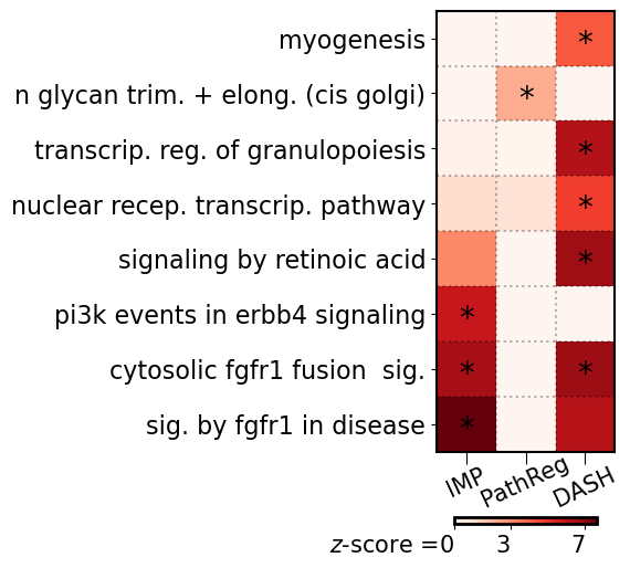
Figure 8: Hematopoesis pathway analysis. We visualize the top-20 significant pathways for each method on the Monocyte lineage of the Hematopoiesis data. For each method (x-axis) we show the pathway z-score and indicate significant results after FWER correction (Bonferroni, p-value cutoff at $.05$) with *.

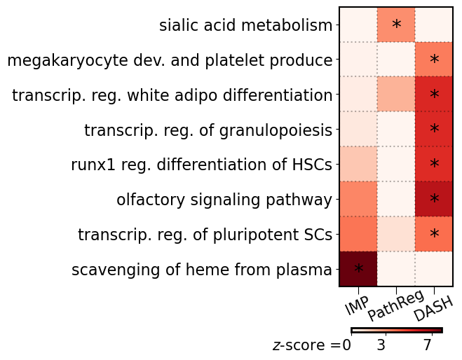
Figure 9: Hematopoesis pathway analysis. We visualize the top-20 significant pathways for each method on the B-cell lineage of the Hematopoiesis data. For each method (x-axis) we show the pathway z-score and indicate significant results after FWER correction (Bonferroni, p-value cutoff at $.05$) with *.

Appendix B Supplementary methods

B.1 Synthetic data generation

The purpose of simulation based data is so that the the underlying dynamical system that produced the this gene expression was known. Do this end, we closely follow the steps outlined by the simulation pipeline provided by Hossain et al. (2023) to generate reliable synthetic time-series gene expression data from two ground truth gene regulatory networks $G_{350}$ and $G_{690}$ consisting of 350 and 690 genes, respectively.

The pipeline adapts SimulatorGRN (Bhuva et al., 2019) to generate from two synthetic S. cerevisiae gene regulatory systems (SIM350 and SIM690, consisting of 350 and 690 genes respectively). For every noise setting $\in\{0\%,5\%,10\%\}$, the connectivity structure of each in silico system is used to synthesize $160$ noisy expression trajectories for each gene across $t\in T=\{0,2,3,7,9\}$. We split up the trajectories into training (88%), validation (6% for tuning $\lambda$), and testing (6%). Since the average simulated expression value is $\approx 0.5$, adding Gaussian noise of $\mathcal{N}(0,\sigma^{2})$ using $\sigma\in\{0,\frac{1}{40},\frac{1}{20}\}$ corresponds roughly to average noise levels of $\{0\%,5\%,10\%\}$.

B.2 Setup for model training

B.2.1 Model complexity

Since the number of genes $n$ in each problem is different, the number of neurons $m$ in PHOENIX’s hidden layer is chosen to roughly scale with this $n$ according to the original paper (Hossain et al., 2023):

• SIM350: $n=350$, $m=40$

• SIM690: $n=690$, $m=50$

• Bone marrow data: $n=529$, $m=50$

• Breast cancer data: $n=11165$, $m=300$

B.2.2 Initialization and optimizers

For initialization values for each of $\text{NN}_{sums}$, $\text{NN}_{prods}$, $\text{NN}_{\Sigma combine}$, and $\text{NN}_{\Pi combine}$, as well as that of $\boldsymbol{\upsilon}_{i}$s we choose the default provided by the PHOENIX implementation (Hossain et al., 2023). The ODESolver (dopri5) and optimizer (Adam) are also chosen as the PHOENIX defaults across all experiments.

B.2.3 Pruning details

We use iterative pruning schedules that are initially very aggressive and then become much more gradual. We found this approach to achieve high sparsity without adversely affecting the training dynamics (and subsequently the validation performance).

• SIM350: prune 70% at epoch 3, and then 10% every 10 epochs

• SIM690: prune 70% at epoch 3, and then 10% every 10 epochs

• Bone marrow data: prune 70% at epoch 3, and then 10% every 10 epochs

• Breast cancer data: prune 90% at epoch 10, and then 10% every 20 epochs

Weight normalization for DASH pruning scores

As described in Section 3, the weight matrices of PHOENIX need to be normalized to $|\widetilde{\boldsymbol{W_{\Sigma}^{(t)}}}|$, $|\widetilde{\boldsymbol{W_{\Pi}^{(t)}}}|$, $|\widetilde{\boldsymbol{U_{\Sigma}^{(t)}}}|$, and $|\widetilde{\boldsymbol{U_{\Pi}^{(t)}}}|$ in the formula for calculating DASH pruning scores $\boldsymbol{\Omega_{\Sigma}},\boldsymbol{\Omega_{\Pi}},\boldsymbol{\Psi_{\Sigma}},\boldsymbol{\Psi_{\Pi}}$. We perform the following normalizations:

• For$|\widetilde{\boldsymbol{W_{\Sigma}^{(t)}}}|$ we simply normalize by taking elementwise absolute values of $\boldsymbol{W_{\Sigma}^{(t)}}$ and dividing all entries by the overall sum of absolute values.

• For $|\widetilde{\boldsymbol{W_{\Pi}^{(t)}}}|$we approach similarly, with the only modification that the weights are elementwise exponentiated instead of elementwise absolute value, given that $\widetilde{\boldsymbol{W_{\Pi}^{(t)}}}$ operates on the log-space.

• For$|\widetilde{\boldsymbol{U_{\Sigma}^{(t)}}}|$ and $|\widetilde{\boldsymbol{U_{\Pi}^{(t)}}}|$ we approach again similarly, with the important modification that the gene-specific multipliers (from Section 4.2) are row-wise multiplied into the weight matrices prior to normalization. This allows the effect of gene multipliers to appropriately be considered when performing pruning.

B.2.4 Learning rates

The learning rate is used as the PHOENIX default of $10^{-3}$. We reduce the learning rate by 10% every 3 epochs, unless the validation set performance shows reasonable improvement. Importantly, we reset the learning rate back to $10^{-3}$ immediately after a pruning step is completed, thereby allowing the newly sparsified model to start learning with a higher learning rate.

B.2.5 Stopping criteria

We train for up to 500 epochs on an AWS c5.9xlarge instance, where each epoch consisted of the entire training set being fed to the model, preceded by any pruning step that is prescribed by the pruning schedule. Training is terminated if the validation set performance fails to improve in 40 consecutive epochs. Upon training termination, we have obtained a model that has been iteratively sparsified to an extent that fails to improve the validation set performance. Hence this training procedure automatically finds an optimal sparsity level using the validation set.

B.3 Prior knowledge to obtain DASH pruning scores

As mentioned in Section 3.2, DASH can leverage prior matrices $\boldsymbol{P}$ and $\boldsymbol{C}$ to inform its pruning score. We use the following in our experiments:

• SIM350 and SIM690:

  • for synthetic experiments we choose $\boldsymbol{P}=\boldsymbol{A^{\sigma_{\%}}}$ to be noisy/corrupted versions (see B.3.1) of the adjacency matrices of ground truth networks $G_{350}$ and $G_{690}$ to reflect that transcription factor binding to target genes can itself be a noisy process in real life. A 1 $\boldsymbol{A^{\sigma_{\%}}}$ represents prior knowledge of an interaction existing between two genes, and a 0 represented no interaction.

  • For $\boldsymbol{C}$ we use the outer product $\boldsymbol{C=\boldsymbol{A^{\sigma_{\%}}}(\boldsymbol{A^{\sigma_{\%}}})^{\intercal}}$, to represent prior knowledge of coregulation. We again applied the corruption/missepecification procedure from B.3.1 so that $\boldsymbol{C}$ is also noisy.

• Breast cancer data:

  • For the prior domain knowledge, we set $\boldsymbol{P}=\boldsymbol{W_{0}}$, where $\boldsymbol{W_{0}}$ was a motif map derived from the human reference genome, for the breast tissue specifically, which we obtained from the work of Weighill et al. (2021). $W_{0}$ is a binary matrix with $\boldsymbol{W_{0}}_{i,j}\in\{0,1\}$ where 1 indicates a TF sequence motif in the promoter of the target gene, and hence indicating a putattive interaction.

  • Also from the work of Weighill et al. (2021) we obtained a protein-protein interaction matrix (PPI) which could use to operationalize our $\boldsymbol{C}$ matrix, since a PPI is a again a binary matrix that is suggestive of which transcription factors have combined (or coregulatory) effects.

• Bone marrow data:

  • For the prior domain knowledge, we followed a similar strategy as the breast cancer analysis, and set $\boldsymbol{P}$ and $\boldsymbol{C}$ based on the motif map and PPI matrix used in Weighill et al. (2021). We appropriately subsetted $\boldsymbol{P}$ and $\boldsymbol{C}$ to only be limited to the $n=529$ genes that were selected by the PathReg authors (Aliee et al., 2022) in the analysis.

B.3.1 Creating corrupted/misspecified prior models for synthetic data

For each noise level $\sigma_{\%}\in\{0\%,5\%,10\%,20\%,40\%,80\%,100\%\}$ in our in silico experiments, we created a shuffled version of $G_{350}$ (and similarly $G_{690}$) where we shuffled $\sigma_{\%}$ of the edges by relocating those edges to new randomly chosen origin and destination genes within the network. This yielded the shuffled network $G_{350}^{\sigma_{\%}}$ (and similarly $G_{690}^{\sigma_{\%}}$) with corresponding adjacency matrix $\boldsymbol{A^{\sigma_{\%}}}$. We set activating edges in $\boldsymbol{A^{\sigma_{\%}}}$ to +1 and repressive edges to -1, and defined the simple linear prior domain knowledge model:

B.4 Validation (choosing $\lambda$) and testing

The choice of $\boldsymbol{\lambda}=(\lambda_{1},\lambda_{2})$ is important for optimally combining prior information with model weights. Hence we implement a $K$-fold cross validation approach to choose $\boldsymbol{\lambda}$. Test set performance is measured as the mean squared error between predictions and held-out expression values in the test set.

B.5 Biological alignment of sparsified models

To validate biological alignment of trained and sparsified models, we extracted GRNs from each models (as explained in C.2), and compared back to the validation networks. Specifically, once we extracted a GRN from the trained model, we looked at how well 0s vs non-zeros in that network aligned with 0s vs non-zeros in the validation network. Our comaprison metric was balanced accuracy, which is the average of the true positive and true negative rates. The validation networks were as follows:

• SIM350, SIM690: We used the ground truth networks $G_{350}$ and $G_{690}$.

• Breast cancer data: We used ChIP-seq data from the MCF7 cell line (breast cancer) in the ReMap2018 database (Chèneby et al., 2018) to create a validation network of TF-target interactions.

• Bone marrow data: As also noted by Aliee et al. (2022), validation network was not available, so we resorted to the pathway analysis.

B.6 Stategy to potentially extend DASH to arbitrary number of layers $L$

Supposing we only have access to prior knowledge in the form of putative prior effect sizes between the $n$ inputs and $o$ outputs $\boldsymbol{P}\in\mathbb{R}^{o\times n}$. Then, for an NN with $L-1$ layers $\boldsymbol{W_{1}}\in\mathbb{R}^{m_{1}\times n},\boldsymbol{W_{2}}\in\mathbb{R}^{m_{2}\times m_{1}},\dots,\boldsymbol{W_{L}}\in\mathbb{R}^{o\times m_{L}}$, we can adopt a strategy where we consider the pruning scores to be fixed for all but one layer.

Since the product $\boldsymbol{W_{L}^{(t)}\dots W_{2}^{(t)}\cdot W_{1}^{(t)}}\in\mathbb{R}^{o\times n}$ represents the overall flow of information from inputs to outputs at epoch $t$, we surmise that $\boldsymbol{\Omega_{L}^{(t)}\dots\Omega_{2}^{(t)}\cdot\Omega_{1}^{(t)}}\in\mathbb{R}^{o\times n}$ should reflect $\boldsymbol{P}$. We can thus prune as follows:

1. Starting with the last layer, we fix the pruning scores of all other layers and compute as follows:

   $$\boldsymbol{\Omega_{L}^{(t)}}:=(1-\lambda_{L})\widetilde{|\boldsymbol{W_{L}^{(t)}}|}+\lambda_{L}\Big{|}\boldsymbol{P}\cdot\texttt{PInv}_{R}\Big{(}\boldsymbol{\Omega^{(t)}_{L-1}\dots\Omega^{(t)}_{2}\Omega^{(t)}_{1}}\Big{)}\Big{|}.$$

2. For the middle layers $l\in\{2,3,\dots,L-1\}$, we do:

   $$\boldsymbol{\Omega_{l}^{(t)}}:=(1-\lambda_{l})\widetilde{|\boldsymbol{W_{l}^{(t)}}|}+\lambda_{l}\Big{|}\texttt{PInv}_{L}\Big{(}\boldsymbol{\Omega^{(t)}_{L}\dots\Omega^{(t)}_{l+2}\Omega^{(t)}_{l+1}}\Big{)}\cdot\boldsymbol{P}\cdot\texttt{PInv}_{R}\Big{(}\boldsymbol{\Omega^{(t)}_{l-1}\dots\Omega^{(t)}_{2}\Omega^{(t)}_{1}}\Big{)}\Big{|}.$$

3. The first layer can be pruned using:

   $$\boldsymbol{\Omega_{1}^{(t)}}:=(1-\lambda_{1})\widetilde{|\boldsymbol{W_{1}^{(t)}}|}+\lambda_{1}\Big{|}\texttt{PInv}_{L}\Big{(}\boldsymbol{\Omega^{(t)}_{L}\dots\Omega^{(t)}_{3}\Omega^{(t)}_{2}}\Big{)}\cdot\boldsymbol{P}\Big{|}.$$

B.7 Processing steps for real data

B.7.1 Breast cancer

The original data set comes from a cross-sectional breast cancer study (GEO accession GSE7390 (Desmedt et al., 2007)) consisting of microarray expression values for 22000 genes from 198 breast cancer patients, that is sorted along a pseudotime axis. We note that the same data set was also ordered in pseudotime by Sun et al. (2021) in the PROB paper. For consistency in pseudotime inference, we obtained the same version of this data that was already preprocessed and sorted by PROB. We normalized the expression values to be between 0 and 1. We limited our analysis to the genes that had measurable expression and appeared in the aforementioned motif map and PPI matrices. This resulted in a pseudotrajectory of expression values for 11165 genes across 186 patients. We removed a contiguous interval of expression across 8 time points for testing (5%), and split up the remaining 178 time points into training (170, $90\%$) and validation for tuning $\lambda_{\text{prior}}$ (8, $5\%$).

B.7.2 Bone marrow

The data is originally from Luecken et al. (2021) (GEO accession code = GSE194122). The cleaning, preprocessing, and pseudotime analysis and was appropriately performed by Aliee et al. (2022) in the PathReg paper, and made publicly available, allowing us to access the processed version. Importantly, Aliee et al. (2022) split up the data into 3 different lineages (Erythroid, Monocyte, and B-Cell), and we fit a separate PHOENIX model on each lineage. The set contains 5 separate batches of data for each lineage, we used 1 for training (batch S1D2), 1 for validation (batch S1D1) and 3 for testing (batches S1D1, S2D4, and S3D6).

B.8 Pathway analyses for breast cancer and bone marrow datasets

We followed very closely the steps below from the Methods section of the PHOENIX paper (Hossain et al., 2023) in order to compute pathway scores, with the only difference that we compute scores between different sparsification strategies Pru.

B.8.1 Gene influence scores

Given $\mathcal{M}_{\texttt{Pru}}$ a PHOENIX model trained on a dataset consisting of $n$ genes, and sparsified using the pruning strategy Pru (for $\texttt{Pru}\in\{\texttt{DASH},\texttt{IMP},\texttt{C-NODE},\dots,\texttt{PathReg}\}$), we performed perturbation analyses to compute gene influence scores $\mathcal{IS}_{\texttt{Pru},j}$. We randomly generated 200 initial ($t=0$) expression vectors via i.i.d standard uniform sampling $\{\boldsymbol{g(0)_{k}}\in\mathbb{R}^{n}\}_{k=1}^{200}$. Next, for each gene $j$ in $\mathcal{M}_{\texttt{Pru}}$, we created a perturbed version of these initial value vectors $\{\boldsymbol{g^{j}(0)_{k}}\}_{k=1}^{200}$, where only gene $j$ was perturbed in each unperturbed vector of $\{\boldsymbol{g(0)_{k}}\}_{k=1}^{200}$. We then fed both sets of initial values into $\mathcal{M}_{\texttt{Pru}}$ to obtain two sets of predicted trajectories $\{\{\boldsymbol{\widehat{g}(t)_{k}}\}_{t\in T}\in\mathbb{R}^{n}\}_{k=1}^{200}$ and $\{\{\boldsymbol{\widehat{g}^{j}(t)_{k}}\}_{t\in T}\in\mathbb{R}^{n}\}_{k=1}^{200}$ across a set of time points $T$. We calculated influence as the average absolute difference between the two sets of predictions, that represented how changes in initial ($t=0$) expression of gene $j$ affected subsequent ($t>0$) predicted expression of all other genes in the Pru-dimensional system

$$\mathcal{IS}_{\texttt{Pru},j}=\frac{1}{200}\sum_{k=1}^{200}\Bigg{[}\frac{1}{\lvert T\rvert}\sum_{\begin{subarray}{c}t\in T\\ t\neq 0\end{subarray}}\Bigg{(}\frac{1}{n}\sum_{\begin{subarray}{c}i=1\\ i\neq j\end{subarray}}^{n}\big{\lvert}\widehat{g_{i}}(t)_{k}-\widehat{g_{i}}^{j}(t)_{k}\big{\lvert}\Bigg{)}\Bigg{]}.$$

B.8.2 Pathway influence scores

Having computed gene influence scores $\mathcal{IS}_{\texttt{Pru},j}$ for each gene $j$ in each dynamical system of dimension $n$ genes sparsified with method Pru, we translated these gene influence scores into pathway influence scores. We used the Reactome pathway data set, GO biological process terms, and GO molecular function terms from MSigDB (Liberzon et al., 2015), that map each biological pathway/process, to the genes that are involved in it. For each system sparsified by Pru, we obtained the pathway ($p$) influence scores ($\mathcal{PS}_{\texttt{Pru},p}$) as the sum of the influence scores of all genes involved in pathway $p$

$$\mathcal{PS}_{\texttt{Pru},p}=\sum_{j\in p}\mathcal{IS}_{\texttt{Pru},j}.$$

We statistically tested whether each pathway influence score is higher than expected by chance using empirical null distributions. We randomly permuted the gene influence scores across the genes to recompute “null” values $\mathcal{PS}^{0}_{\texttt{Pru},p}$. For each pathway, we performed $K=1000$ permutations to obtain a null distribution $\{\mathcal{PS}^{0}_{\texttt{Pru},p,k}\}_{k=1}^{K}$ that can be compared to $\mathcal{PS}_{\texttt{Pru},p}$. We could then compute an empirical $p$-value as $p=\frac{1}{K}\sum_{k=1}^{K}\mathbb{I}_{\mathcal{PS}^{0}_{\texttt{Pru},p,k}>\mathcal{PS}_{\texttt{Pru},p}}$, where $\mathbb{I}$ is the indicator function. Finally, we used the mean ($\mu_{0(\texttt{Pru},p)}$) and variance ($\sigma^{2}_{0(\texttt{Pru},p)}$) of the null distribution $\{\mathcal{PS}^{0}_{\texttt{Pru},p,k}\}_{k=1}^{K}$ to obtain and visualize pathway $z$-scores that are now comparable across pathways ($p$) and sparsification strategies (Pru)

$$z_{(\texttt{Pru},p)}=\frac{\mathcal{PS}_{\texttt{Pru},p}-\mu_{0(\texttt{Pru},p)}}{\sqrt{\sigma^{2}_{0(\texttt{Pru},p)}}}.$$

B.9 Implementation details for other sparsification strategies on the PHOENIX architecture

B.9.1 Iterative magnitude pruning

As discussed in Section 3.4, IMP can be operationalized as a special case of DASH by setting $\lambda_{1}=\lambda_{2}=0$.

B.9.2 Post hoc + Finetune

Once a PHOENIX model is fully trained (without any pruning), we inspect the trained model and pruned the lowest $p\%$ of parameters in each of $\boldsymbol{W_{\Sigma}},\boldsymbol{W_{\Pi}},\boldsymbol{U_{\Sigma}},\boldsymbol{U_{\Pi}}$ based on on the normalized weights (see B.2) to 0. We then fine-tune (i.e retrain without training the pruned parameters) this $p\%$ sparsified model and calculate its performance on the validation set. We repeat this process for a grid of values for $p\in\{0.50,0.75,0.83,0.87,0.90,0.92,0.95,0.97,0.99\}$. The validation set can then inform the best value of $p$. We repeated this entire procedure 3 times, so that we could apply the 1 standard error rule (Hastie et al., 2009) and choose the optimal $p$ as the sparsest fine-tuned model whose validation MSE is within 1 standard error of lowest obtained average validation MSE.

B.9.3 Penalty based methods

C-NODE, PathReg, and $L_{0}$ implementations were obtained from the code associated with the PathReg paper (Aliee et al., 2022). We adapted the code so that the base NN architecture was exactly that of the PHOENIX model, including an implementation of the gene-specific multipliers (from Section 4.2). Finally, we tuned the relevant parameters $\lambda_{0}$ and $\lambda_{1}$ in the objective function using the validation set.

Appendix C PHOENIX NeuralODE model - additional details

These details are borrowed from Hossain et al. (2023)’s paper, and provided here for the reader’s convenience.

C.1 Prior knowledge incorporation in base PHOENIX model itself

PHOENIX has the option to promote the NeuralODE to flexibly align with structural domain knowledge, while still explaining the observed gene expression data. This is operationalized via a modified loss function

$$\mathcal{L}_{\text{mod}}\Big{(}\boldsymbol{g}(t_{1}),\widehat{\boldsymbol{g}(t_{1})}\Big{)}=\tau\overbrace{L\Big{(}\boldsymbol{g}(t_{1})~{}\boldsymbol{;}~{}\boldsymbol{g}(t_{0})+\int_{t_{0}}^{t_{1}}\text{NN}_{\Theta}(\boldsymbol{g}(t_{1}),t)~{}dt\Big{)}}^{\text{loss based on matching observed gene expression data}}+(1-\tau)\overbrace{L\Big{(}\mathcal{P^{*}}\big{(}\boldsymbol{g}(t_{1})\big{)}~{}\boldsymbol{;}~{}\text{NN}_{\Theta}(\boldsymbol{g}(t_{1}),t)\Big{)}}^{\text{loss based on matching domain-knowledge}}$$

that incorporates the effect of any user-provided prior model $\mathcal{P^{*}}$, using a tuning parameter $\tau$, and the original loss function $L(\boldsymbol{x},\widehat{\boldsymbol{x}})$. PHOENIX implements $\mathcal{P^{*}}$ as a simple linear model $\mathcal{P^{*}}\big{(}\boldsymbol{\gamma_{k}}\big{)}=\boldsymbol{A}\cdot\boldsymbol{\gamma_{k}}-\boldsymbol{\gamma_{k}}$, where $\boldsymbol{A}$ is the adjacency matrix of likely connectivity structure based on prior domain knowledge (such as experimentally validated interactions) with $\boldsymbol{A}_{ij}\in\{+1,-1,0\}$ representing an activating, repressive, or no prior interaction, respectively.

Note: We switched this prior-informed regularizer on for baselines, as it yielded better, sparser results, but off for any pruning approaches, as it showed detrimental performance (see App. Tab. 6). For synthetic experiments, we used the simple linear model: $\mathcal{P^{*}}\big{(}\boldsymbol{\gamma_{k}}\big{)}=\boldsymbol{A^{\sigma_{\%}}}\cdot\boldsymbol{\gamma_{k}}-\boldsymbol{\gamma_{k}}$, where we chose $\boldsymbol{A^{\sigma_{\%}}}$ to be noisy/corrupted versions of the adjacency matrices of ground truth networks $G_{350}$ and $G_{690}$ (details in B.3.1). We set activating edges in $\boldsymbol{A^{\sigma_{\%}}}$ to +1 and repressive edges to -1. “No interaction” was represented using 0.

C.2 Algorithm for efficiently retrieving encoded GRN from trained PHOENIX model

We start with PHOENIX’s prediction for the local derivative given a gene expression vector $\boldsymbol{g}(t)\in\mathbb{R}^{n}$ in an $n$-gene system:

$$\widehat{\frac{d\boldsymbol{g}(t)}{dt}}=\text{ReLU}(\boldsymbol{\upsilon})\odot\Big{[}\boldsymbol{W}_{\cup}\{\boldsymbol{c_{\Sigma}}(\boldsymbol{g}(t))\oplus\boldsymbol{c_{\Pi}}(\boldsymbol{g}(t))\}-\boldsymbol{g}(t)\Big{]},~{}~{}\text{where}$$

$$\boldsymbol{c_{\Sigma}}(\boldsymbol{g}(t))=\boldsymbol{W_{\Sigma}}\phi_{\Sigma}(\boldsymbol{g}(t))+\boldsymbol{b_{\Sigma}}~{}~{}\text{ and }~{}~{}\boldsymbol{c_{\Pi}}(\boldsymbol{g}(t))=\exp\circ(\boldsymbol{W_{\Pi}}\phi_{\Pi}(\boldsymbol{g}(t))+\boldsymbol{b_{\Pi}})$$

A trained PHOENIX model encodes interactions between genes primarily within the gene-specific multipliers $\boldsymbol{\upsilon}\in\mathbb{R}^{n}$, and the weight parameters from its neural network blocks $\boldsymbol{W_{\Pi}},\boldsymbol{W_{\Sigma}}\in\mathbb{R}^{m\times n}$ and $\boldsymbol{W}_{\cup}\in\mathbb{R}^{n\times 2m}$. This inspired an efficient means of projecting the estimated dynamical system down to a gene regulatory network (GRN) $\widehat{G_{n}}$. In particular a matrix $\boldsymbol{D}\in\mathbb{R}^{n\times n}$ is calculated, where $\boldsymbol{D}_{ij}$ approximated the absolute contribution of gene $j$ to the derivative of gene $i$’s expression:

$$\boldsymbol{D}=\boldsymbol{W}_{\cup}\begin{bmatrix}\boldsymbol{W_{\Sigma}}\\ \boldsymbol{W_{\Pi}}\end{bmatrix}$$

Gene-specific multipliers $\boldsymbol{\upsilon}$ are applied, before adapting the marginal attribution approach described by Hackett et al. (Hackett et al., 2020). This resulted in the dynamics matrix $\widetilde{\boldsymbol{D}}$ where $\widetilde{\boldsymbol{D}_{ij}}$ was scaled according to the relative contribution of gene $j$ to the rate of change in gene $i$’s expression:

$$\widetilde{\boldsymbol{D}_{ij}}=\frac{\boldsymbol{\upsilon}_{i}\boldsymbol{D}_{ij}}{\sum_{j^{\prime}=1}^{n}\lvert\boldsymbol{\upsilon}_{i}\boldsymbol{D}_{ij^{\prime}}\lvert}.$$

References

- Aliee et al. (2021) Aliee, H., Theis, F. J., and Kilbertus, N. Beyond predictions in neural odes: Identification and interventions. arXiv preprint arXiv:2106.12430, 2021.
- Aliee et al. (2022) Aliee, H., Richter, T., Solonin, M., Ibarra, I., Theis, F., and Kilbertus, N. Sparsity in continuous-depth neural networks. Advances in Neural Information Processing Systems, 35:901–914, 2022.
- Arora et al. (2018) Arora, S., Cohen, N., and Hazan, E. On the optimization of deep networks: Implicit acceleration by overparameterization. In International Conference on Machine Learning, pp. 244–253, 2018.
- Bhuva et al. (2019) Bhuva, D. D., Cursons, J., Smyth, G. K., and Davis, M. J. Differential co-expression-based detection of conditional relationships in transcriptional data: comparative analysis and application to breast cancer. Genome biology, 20(1):1–21, 2019.
- Burkholz (2022) Burkholz, R. Most activation functions can win the lottery without excessive depth. In Advances in Neural Information Processing Systems, 2022.
- Busiello et al. (2017) Busiello, D. M., Suweis, S., Hidalgo, J., and Maritan, A. Explorability and the origin of network sparsity in living systems. Scientific reports, 7(1):12323, 2017.
- Cao et al. (2003) Cao, Y., Li, S., Petzold, L., and Serban, R. Adjoint sensitivity analysis for differential-algebraic equations: The adjoint dae system and its numerical solution. SIAM journal on scientific computing, 24(3):1076–1089, 2003.
- Chang et al. (2021) Chang, X., Li, Y., Oymak, S., and Thrampoulidis, C. Provable benefits of overparameterization in model compression: From double descent to pruning neural networks. In Proceedings of the AAAI Conference on Artificial Intelligence, volume 35, pp. 6974–6983, 2021.
- Chen et al. (2018) Chen, R. T., Rubanova, Y., Bettencourt, J., and Duvenaud, D. K. Neural ordinary differential equations. Advances in neural information processing systems, 31, 2018.
- Chen et al. (2022) Chen, Z., King, W. C., Hwang, A., Gerstein, M., and Zhang, J. Deepvelo: Single-cell transcriptomic deep velocity field learning with neural ordinary differential equations. Science Advances, 8(48):eabq3745, 2022.
- Chèneby et al. (2018) Chèneby, J., Gheorghe, M., Artufel, M., Mathelier, A., and Ballester, B. Remap 2018: an updated atlas of regulatory regions from an integrative analysis of dna-binding chip-seq experiments. Nucleic acids research, 46(D1):D267–D275, 2018.
- Cybenko (1989) Cybenko, G. Approximation by superpositions of a sigmoidal function. Math. Control. Signals Syst., 2(4):303–314, 1989. doi: 10.1007/BF02551274. URL https://doi.org/10.1007/BF02551274.
- da Cunha et al. (2022) da Cunha, A., Natale, E., and Viennot, L. Proving the lottery ticket hypothesis for convolutional neural networks. In International Conference on Learning Representations, 2022.
- Degrave et al. (2022) Degrave, J., Felici, F., Buchli, J., Neunert, M., Tracey, B., Carpanese, F., Ewalds, T., Hafner, R., Abdolmaleki, A., de Las Casas, D., Donner, C., Fritz, L., Galperti, C., Huber, A., Keeling, J., Tsimpoukelli, M., Kay, J., Merle, A., Moret, J. M., Noury, S., Pesamosca, F., Pfau, D., Sauter, O., Sommariva, C., Coda, S., Duval, B., Fasoli, A., Kohli, P., Kavukcuoglu, K., Hassabis, D., and Riedmiller, M. Magnetic control of tokamak plasmas through deep reinforcement learning. Nature, 602(7897):414–419, Feb 2022.
- Desmedt et al. (2007) Desmedt, C., Piette, F., Loi, S., Wang, Y., Lallemand, F., Haibe-Kains, B., Viale, G., Delorenzi, M., Zhang, Y., d’Assignies, M. S., et al. Strong time dependence of the 76-gene prognostic signature for node-negative breast cancer patients in the transbig multicenter independent validation series. Clinical cancer research, 13(11):3207–3214, 2007.
- Erbe et al. (2023) Erbe, R., Stein-O’Brien, G., and Fertig, E. J. Transcriptomic forecasting with neural ordinary differential equations. Patterns, 4(8), 2023.
- Ferbach et al. (2023) Ferbach, D., Tsirigotis, C., Gidel, G., and Bose, J. A general framework for proving the equivariant strong lottery ticket hypothesis. In International Conference on Learning Representations, 2023.
- Fischer & Burkholz (2022) Fischer, J. and Burkholz, R. Plant ’n’ seek: Can you find the winning ticket? In International Conference on Learning Representations, 2022.
- Fischer et al. (2021) Fischer, J., Gadhikar, A. H., and Burkholz, R. Towards strong pruning for lottery tickets with non-zero biases. arXiv preprint arXiv:2110.11150, 2021.
- Frankle & Carbin (2018) Frankle, J. and Carbin, M. The lottery ticket hypothesis: Finding sparse, trainable neural networks. arXiv preprint arXiv:1803.03635, 2018.
- Frankle et al. (2021) Frankle, J., Dziugaite, G. K., Roy, D., and Carbin, M. Pruning neural networks at initialization: Why are we missing the mark? In International Conference on Learning Representations, 2021. URL https://openreview.net/forum?id=Ig-VyQc-MLK.
- Gadhikar & Burholz (2024) Gadhikar, A. H. and Burholz, R. Masks, signs, and learning rate rewinding. In International Conference on Learning Representations, 2024.
- Hackett et al. (2020) Hackett, S. R., Baltz, E. A., Coram, M., Wranik, B. J., Kim, G., Baker, A., Fan, M., Hendrickson, D. G., Berndl, M., and McIsaac, R. S. Learning causal networks using inducible transcription factors and transcriptome-wide time series. Mol Syst Biol, 16(3):e9174, Mar 2020.
- Hastie et al. (2009) Hastie, T., Tibshirani, R., Friedman, J. H., and Friedman, J. H. The elements of statistical learning: data mining, inference, and prediction, volume 2. Springer, 2009.
- Hossain et al. (2023) Hossain, I., Fanfani, V., Fischer, J., Quackenbush, J., and Burkholz, R. Biologically informed NeuralODEs for genome-wide regulatory dynamics. bioRxiv, pp. 2023–02, 2023.
- Jiramongkol & Lam (2020) Jiramongkol, Y. and Lam, E. W. FOXO transcription factor family in cancer and metastasis. Cancer Metastasis Rev, 39(3):681–709, Sep 2020.
- Jumper et al. (2021) Jumper, J., Evans, R., Pritzel, A., Green, T., Figurnov, M., Ronneberger, O., Tunyasuvunakool, K., Bates, R., dek, A., Potapenko, A., Bridgland, A., Meyer, C., Kohl, S. A. A., Ballard, A. J., Cowie, A., Romera-Paredes, B., Nikolov, S., Jain, R., Adler, J., Back, T., Petersen, S., Reiman, D., Clancy, E., Zielinski, M., Steinegger, M., Pacholska, M., Berghammer, T., Bodenstein, S., Silver, D., Vinyals, O., Senior, A. W., Kavukcuoglu, K., Kohli, P., and Hassabis, D. Highly accurate protein structure prediction with AlphaFold. Nature, 596(7873):583–589, Aug 2021.
- Kusupati et al. (2020) Kusupati, A., Ramanujan, V., Somani, R., Wortsman, M., Jain, P., Kakade, S., and Farhadi, A. Soft threshold weight reparameterization for learnable sparsity. In International Conference on Machine Learning, pp. 5544–5555. PMLR, 2020.
- Li (2023) Li, Q. sctour: a deep learning architecture for robust inference and accurate prediction of cellular dynamics. Genome Biology, 24(1):1–33, 2023.
- Liberzon et al. (2015) Liberzon, A., Birger, C., Thorvaldsdóttir, H., Ghandi, M., Mesirov, J. P., and Tamayo, P. The molecular signatures database hallmark gene set collection. Cell systems, 1(6):417–425, 2015.
- Liebenwein et al. (2021) Liebenwein, L., Hasani, R., Amini, A., and Rus, D. Sparse flows: Pruning continuous-depth models. Advances in Neural Information Processing Systems, 34:22628–22642, 2021.
- Liu et al. (2020) Liu, J., Xu, Z., Shi, R., Cheung, R. C. C., and So, H. K. Dynamic sparse training: Find efficient sparse network from scratch with trainable masked layers. In International Conference on Learning Representations, 2020. URL https://openreview.net/forum?id=SJlbGJrtDB.
- Liu et al. (2022) Liu, R., Pisco, A. O., Braun, E., Linnarsson, S., and Zou, J. Dynamical systems model of rna velocity improves inference of single-cell trajectory, pseudo-time and gene regulation. Journal of Molecular Biology, 434(15):167606, 2022.
- Liu et al. (2023) Liu, Z., Gan, E., and Tegmark, M. Seeing Is Believing: Brain-Inspired Modular Training for Mechanistic Interpretability. Entropy (Basel), 26(1), Dec 2023.
- Louizos et al. (2017) Louizos, C., Welling, M., and Kingma, D. P. Learning sparse neural networks through regularization. arXiv preprint arXiv:1712.01312, 2017.
- Louizos et al. (2018) Louizos, C., Welling, M., and Kingma, D. P. Learning sparse neural networks through l_0 regularization. In International Conference on Learning Representations, 2018.
- Luecken et al. (2021) Luecken, M. D., Burkhardt, D. B., Cannoodt, R., Lance, C., Agrawal, A., Aliee, H., Chen, A. T., Deconinck, L., Detweiler, A. M., Granados, A. A., et al. A sandbox for prediction and integration of dna, rna, and proteins in single cells. In 35th Conference on Neural Information Processing Systems (NeurIPS 2021) Track on Datasets and Benchmarks, 2021.
- Malach et al. (2020) Malach, E., Yehudai, G., Shalev-Schwartz, S., and Shamir, O. Proving the lottery ticket hypothesis: Pruning is all you need. In III, H. D. and Singh, A. (eds.), Proceedings of the 37th International Conference on Machine Learning, volume 119 of Proceedings of Machine Learning Research, pp. 6682–6691. PMLR, 13–18 Jul 2020. URL https://proceedings.mlr.press/v119/malach20a.html.
- Marvalim et al. (2023) Marvalim, C., Datta, A., and Lee, S. C. Role of p53 in breast cancer progression: An insight into p53 targeted therapy. Theranostics, 13(4):1421–1442, 2023.
- Mendes et al. (2009) Mendes, P., Hoops, S., Sahle, S., Gauges, R., Dada, J., and Kummer, U. Computational modeling of biochemical networks using copasi. Systems Biology, pp. 17–59, 2009.
- Orseau et al. (2020) Orseau, L., Hutter, M., and Rivasplata, O. Logarithmic pruning is all you need. In Advances in Neural Information Processing Systems, 2020.
- Paul et al. (2023) Paul, M., Chen, F., Larsen, B. W., Frankle, J., Ganguli, S., and Dziugaite, G. K. Unmasking the lottery ticket hypothesis: What’s encoded in a winning ticket’s mask? In International Conference on Learning Representations, 2023.
- Pensia et al. (2020) Pensia, A., Rajput, S., Nagle, A., Vishwakarma, H., and Papailiopoulos, D. Optimal lottery tickets via subset sum: Logarithmic over-parameterization is sufficient. In Advances in Neural Information Processing Systems, volume 33, pp. 2599–2610, 2020.
- Qiu et al. (2022) Qiu, X., Zhang, Y., Martin-Rufino, J. D., Weng, C., Hosseinzadeh, S., Yang, D., Pogson, A. N., Hein, M. Y., Min, K. H. J., Wang, L., et al. Mapping transcriptomic vector fields of single cells. Cell, 185(4):690–711, 2022.
- Ramanujan et al. (2020) Ramanujan, V., Wortsman, M., Kembhavi, A., Farhadi, A., and Rastegari, M. What’s hidden in a randomly weighted neural network? In Conference on Computer Vision and Pattern Recognition, 2020.
- Savarese et al. (2020) Savarese, P., Silva, H., and Maire, M. Winning the lottery with continuous sparsification. In Advances in Neural Information Processing Systems, 2020.
- Sreenivasan et al. (2022) Sreenivasan, K., yong Sohn, J., Yang, L., Grinde, M., Nagle, A., Wang, H., Xing, E., Lee, K., and Papailiopoulos, D. Rare gems: Finding lottery tickets at initialization. In Advances in Neural Information Processing Systems, 2022.
- Sun et al. (2021) Sun, X., Zhang, J., and Nie, Q. Inferring latent temporal progression and regulatory networks from cross-sectional transcriptomic data of cancer samples. PLoS Comput Biol, 17(3):e1008379, Mar 2021.
- Tong et al. (2023) Tong, A., Kuchroo, M., Gupta, S., Venkat, A., Perez San Juan, B., Rangel, L., Zhu, B., Lock, J. G., Chaffer, C., and Krishnaswamy, S. Learning transcriptional and regulatory dynamics driving cancer cell plasticity using neural ode-based optimal transport. bioRxiv, pp. 2023–03, 2023.
- Weighill et al. (2021) Weighill, D., Guebila, M. B., Lopes-Ramos, C., Glass, K., Quackenbush, J., Platig, J., and Burkholz, R. Gene regulatory network inference as relaxed graph matching. AAAI Conference on Artificial Intelligence, 2021.
- Yeo et al. (2021) Yeo, G. H. T., Saksena, S. D., and Gifford, D. K. Generative modeling of single-cell time series with prescient enables prediction of cell trajectories with interventions. Nature communications, 12(1):3222, 2021.
- Zhou et al. (2019) Zhou, H., Lan, J., Liu, R., and Yosinski, J. Deconstructing lottery tickets: Zeros, signs, and the supermask. In Advances in Neural Information Processing Systems, pp. 3597–3607, 2019.