Abstract

With the rapid adoption of Federated Learning (FL) as the training and tuning protocol for applications utilizing Large Language Models (LLMs), recent research highlights the need for significant modifications to FL to accommodate the large-scale of LLMs. While substantial adjustments to the protocol have been introduced as a response, comprehensive privacy analysis for the adapted FL protocol is currently lacking.

To address this gap, our work delves into an extensive examination of the privacy analysis of FL when used for training LLMs, both from theoretical and practical perspectives. In particular, we design two active membership inference attacks with guaranteed theoretical success rates to assess the privacy leakages of various adapted FL configurations. Our theoretical findings are translated into practical attacks, revealing substantial privacy vulnerabilities in popular LLMs, including BERT, RoBERTa, DistilBERT, and OpenAI’s GPTs, across multiple real-world language datasets. Additionally, we conduct thorough experiments to evaluate the privacy leakage of these models when data is protected by state-of-the-art differential privacy (DP) mechanisms.

1 INTRODUCTION

Recent years have observed the exceptional capabilities of Large Language Models (LLMs) (Taylor et al., 2022) in many complex real-world applications, especially those involving AI-generated conversations of ChatGPT (OpenAI, 2023) and Google Bard (Google, 2023). This has spurred significant research efforts in training and utilizing LLMs in various important domains across multiple industries (Huang et al., 2023; Wu et al., 2023; Singhal et al., 2023; Liu et al., 2023). Nevertheless, the success of LLMs comes at the cost of massive amounts of training data as well as computational resources. In response, many recent research (Houlsby et al., 2019; Hu et al., 2022; Li and Liang, 2021; Ben Zaken et al., 2022) independently propose the usage of Federated Learning (FL) (McMahan et al., 2016; Kairouz et al., 2019) to resolve those challenges as it allows the utilization of private data and distributed resources.

Due to the massive size of LLMs, directly training or fine-tuning them for down-stream tasks on FL would cause substantial communication overhead and place heavy burdens on the storage and computational resources of participating devices (Hu et al., 2022; Zhang et al., 2023; Chen et al., 2023). A natural solution for the issues, known as parameter-efficient training and tuning (PET) (Zhang et al., 2023), is to update only a small number of the parameters while freezing the rest (Fig. 1). The PET methods either inject some additional trainable parameters (Li and Liang, 2021), introduce some extra layers (Houlsby et al., 2019; Hu et al., 2022), or update only some portions of the original LLMs (Ben Zaken et al., 2022). These studies have shown the modified FL can achieve comparable performance to traditional FL; nevertheless, a critical gap remains in terms of privacy analysis for these novel protocols. While the overall reduction in communication messages can potentially lower the attack surface, it remains uncertain whether the modified FL methods offer enhanced security as the introduction of extra layers and parameters may introduce new vulnerabilities.

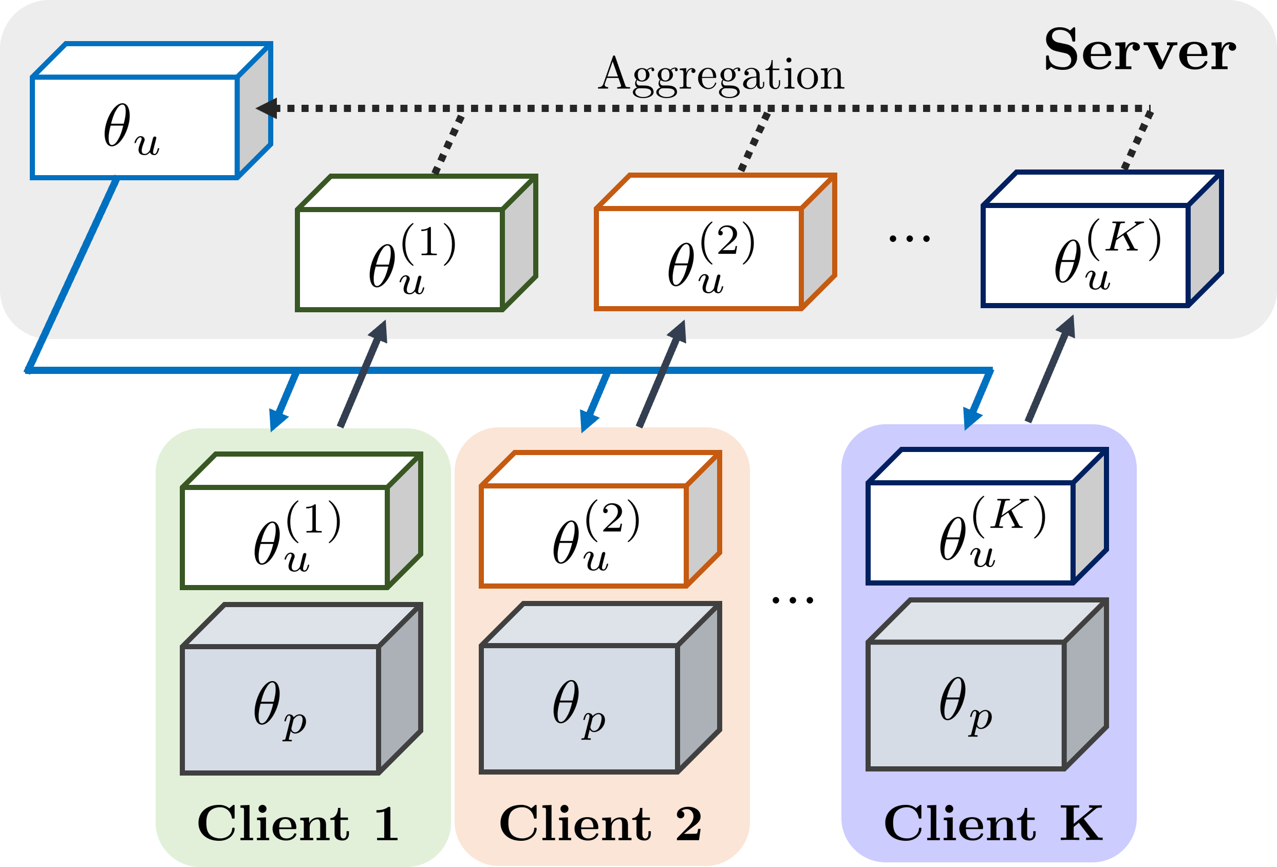
Figure 1: Training/tuning LLMs in FL: The clients typically exchange a light amount of trainable parameters $\theta_{i}$ while keeping most parameters, i.e., $\theta_{p}$, frozen.

Motivated by that lack of study, this paper investigates the privacy leakage in the adoption of FL to LLMs from both theoretical and practical perspectives. Our study focuses on the active setting, wherein the FL server operates dishonestly by manipulating the trainable weights to compromise privacy. Our findings reveal that clients’ data are fundamentally vulnerable to active membership inference (AMI) carried out by a dishonest server. The theme of our study is the construction of low-complexity adversaries with provable high attack success rates. As we will demonstrate in our theoretical results, establishing complexity bounds for these adversaries is imperative as it forms the foundation for rigorous security/privacy statements about the protocol. The challenges are not only in determining the sweet spots between adversaries’ complexity and the attacking success rates but also in showing how the theoretical vulnerabilities manifest as practical risks in the context of FLs for LLMs. For that purpose, our attacks are designed to exploit the trainable fully connected (FC) layers and self-attention layers in FL updates as both are widely adopted to utilize LLMs. Our main contributions are summarized as follows:

• We prove that the server can exploit the FC layers to perfectly infer membership information of local training data (Theorem 1) in FL with LLMs.

• When the trainable weights belong to a self-attention layer, we introduce a sefl-attention-based AMI attack with a significantly high guarantee success rate and demonstrate a similar privacy risk as in the case of FC layers (Theorem 2).

• Practical privacy risks of utilizing LLMs in FL to AMI are demonstrated through the implementations of the formulated adversaries. Our experiments are conducted on five state-of-the-art LLMs, including BERT-based (Devlin et al., 2019; Liu et al., 2019; Sanh et al., 2019) and GPT models (Radford et al., 2019; Brown et al., 2020) on four different datasets. We heuristically assess the privacy risks for both unprotected and Differential Privacy protected data.

Organization. Sect. 2 discusses the background, the related works, and the notations used in this manuscript. Sect. 3 describes the AMI threat models. Sects. 4 provide the descriptions of our attacks and their theoretical analysis. Sect. 5 reports our experimental results and Sect. 6 concludes this paper.

2 BACKGROUND, RELATED WORKS, AND NOTATIONS

This section provides the background, related works, and notations that we use in this work.

Federated Learning (FL). FL (Kairouz et al., 2019) is a collaborative learning framework that allows model updates across decentralized devices while keeping the data localized. The training is typically orchestrated by a central server. At the beginning, the server initializes the model’s parameters. For each training iteration, a subset of clients is selected to participate. Each of them computes the gradients of trainable parameters on its local data. The gradients are then aggregated among the selected clients. The model’s parameters are then updated based on the aggregated gradients. The training continues until convergence.

Parameter-Efficient Training and Tuning. There has been a notable increase in research on PET to avoid full model updates in FL. Generally, these methods focus on updating lightweight trainable parameters while keeping the rest frozen. For instance, the adapter approach (Houlsby et al., 2019; Pfeiffer et al., 2020) inserts two adapter layers to each Transformer block (Vaswani et al., 2017). The computation can be described formally as $h\leftarrow W_{u}\sigma(W_{d}h)$, where $\sigma$ is the nonlinear activation function. Reparameterization-based methods such as LoRA (Hu et al., 2022) aim to optimize the low-rank decomposition for weight update matrices. On the other hand, BitFit (Ben Zaken et al., 2022) empirically demonstrates that only updating the bias terms can still lead to competitive performance. Another common approach is prompt-tuning (Li and Liang, 2021) which attaches trainable vectors, namely prompt, to the model’s input.

Attention mechanism in FL. The Attention mechanism is a machine learning technique that allows a model to focus on specific parts of the input. It has been widely used in machine translation, video processing, speech recognition, and many other applications. Some popular models using attention mechanisms are Transformer (Vaswani et al., 2017), BERT (Devlin et al., 2019), RoBERTa (Liu et al., 2019), and GPTs (Radford et al., 2019; Brown et al., 2020). With its popularity, it is increasingly common to find attention mechanisms in models trained in FL settings, e.g. models of Google (Shah et al., 2020; Yang et al., 2018; Beaufays et al., 2019), Amazon (Roosta et al., 2021), and many others (Stremmel and Singh, 2021; Chen et al., 2020; Bui et al., 2019).

FL with Differential Privacy. Differential Privacy (DP) (Dwork et al., 2006; Erlingsson et al., 2014) has been recognized as a solution to mitigate the privacy risks of gradient sharing in FL. The principle of DP is based on randomized response (Warner, 1965), initially introduced to maintain the confidentiality of survey respondents. The definition of $\varepsilon$-DP is:

Definition 1.

$\varepsilon$-DP. A randomized algorithm $\mathcal{M}$ fulfills $\varepsilon$-DP, if for all subset $\mathcal{S}\subseteq\textup{Range}(\mathcal{M})$ and for any adjacent datasets $D$ and $D^{\prime}$, we have: $Pr[\mathcal{M}(D)\in\mathcal{S}]\leq e^{\varepsilon}Pr[\mathcal{M}(D^{\prime})\in\mathcal{S}]$, where $\varepsilon$ is a privacy budget.

The privacy budget $\varepsilon$ controls the privacy level: a smaller $\varepsilon$ enforces a stronger privacy guarantee; however, it reduces data utility as the distortion is larger.

Related works. The first AMI attack by a dishonest server in FL was recently introduced by Nasr et al. (2019). The attack relies on multiple model updates for inference. Later, the work (Nguyen et al., 2023) introduces a stronger and stealthier attack requiring only one FL iteration; however, a separate neural network trained on the dataset is needed. Both attacks have non-trivial time complexity and provide no theoretical guarantees. Furthermore, neither of these works is tailored for FL with LLMs, and their efficacy in this context has not been validated.

During our research, we noticed related privacy concerns regarding FL with LLMs. The work of Wang et al. (2023) and Yu et al. (2023) explore differentially private FL with LLMs, primarily focusing on assessing the model’s performance while assuming privacy budgets. In contrast, our goal is to analyze new attack vectors in modified FL for LLMs through novel adversarial inference schemes.

Another line of related work focuses on inference attacks, where the attackers aim to deduce the private features of clients in FL (Hitaj et al., 2017; Zhu et al., 2019; Wu et al., 2019; Jin et al., 2021). While inference attacks can be considered as more potent than membership inferences since they can recover the entire input, their effectiveness heavily relies on the training model and method-specific optimizations. These dependencies hinder the establishment of theoretical guarantees of inference attacks. In contrast, membership inferences enable us to circumvent these dependencies, a crucial aspect for establishing Theorems 1 and 2, which provide formal statements regarding the vulnerability of Federated LLMs.

Notations. We consider the private data $D$ in LLMs consists of 2-dimensional arrays, and write $D=\{X_{i}\}_{i=1}^{n}$ for $X_{i}\in\mathcal{X}$ where $\mathcal{X}\subseteq\mathbb{R}^{d_{X}\times l_{X}}$. We use $\mathcal{D}$ to denote the data distribution. Each column of a 2-dimensional array $X$, denoted by $x_{j}\in\mathbb{R}^{d_{X}}$, is referred as a token. We also denote $M$ as the largest $L_{2}$ norm of the tokens, i.e., $M=\max_{X\in D}\max_{x_{j}\in X}\|x_{j}\|$.

Regarding the self-attention mechanisms, for an input $X\in\mathbb{R}^{d_{X}\times l_{X}}$, the layer’s output $Z^{h}\in\mathbb{R}^{d_{\textup{hid}}\times l_{X}}$ of the attention head $h$ is given by:

$$Z^{h} =W_{V}^{h}X\textup{softmax}\left(\nicefrac{{1}}{{\sqrt{d_{\textup{attn}}}}}\ X^{\top}{W_{K}^{h\top}}W_{Q}^{h}X\right)$$ (1)

where $W_{Q}^{h}\in\mathbb{R}^{{d_{\textup{attn}}}\times d_{X}},W_{K}^{h}\in\mathbb{R}^{{d_{\textup{attn}}}\times d_{X}}$ and $W_{V}^{h}\in\mathbb{R}^{d_{\textup{hid}}\times d_{X}}$ are the trainable weights of the head $h$. The output of the layer after ReLU activation is $Y=\textup{ReLU}\left(\sum\nolimits_{h=1}^{H}W_{O}^{h}Z^{h}+b_{O}1^{\top}\right)$ where $H$ is the number of heads, $W_{O}^{h}\in\mathbb{R}^{d_{Y}\times d_{\textup{hid}}}$ are the trainable weights and $b_{O}\in\mathbb{R}^{d_{Y}}$ are the trainable biases for the aggregation of the layer’s final output.

3 THE THREAT MODEL

As the FL server defines the model’s architecture and distributes the parameters, it can deviate from the protocol to strengthen the privacy attacks (Boenisch et al., 2021; Nguyen et al., 2022; Fowl et al., 2021). We formalize our study on the security of FL with LLMs via a security game denoted by AMI Security Game in Subsect. 3.1. In the game, a dishonest server maliciously specifies the model’s architecture and modifies its parameters to infer information about the local training data of a client. We then discuss how the AMI security game can capture the security threat of FL with LLMs in Subsect. 3.2.

3.1 AMI Security Games

$\mathsf{Exp}^{\textup{AMI}}{(\mathcal{A})}$:

# Simulating client’s dataset

$D\leftarrow\emptyset$

while $|D|<n$ do

      $X{\>\stackrel{{\scriptstyle{\scriptscriptstyle\hskip 0.99998pt\mathcal{D}}}}{{\leftarrow}}\>}\mathcal{X}$ # Sampling from data distribution
if $X\notin D$ then

            $D\leftarrow D\cup\{X\}$

      

# The random bit game
$b{\>\stackrel{{\scriptstyle{\scriptscriptstyle\hskip 0.99998pt\$}}}{{\leftarrow}}\>}{\{0,1\}}$, $X\leftarrow\textsc{None}$
if $b=1$ then

       $T{\>\stackrel{{\scriptstyle{\scriptscriptstyle\hskip 0.99998pt\$}}}{{\leftarrow}}\>}D$ # Uniformly sampling

else

       while $T==\textsc{None}$ or $T\in D$ do

             $T{\>\stackrel{{\scriptstyle{\scriptscriptstyle\hskip 0.99998pt\mathcal{D}}}}{{\leftarrow}}\>}\mathcal{X}$ # Sampling from data distribution

      

# The attack
$\Phi\leftarrow\mathcal{A}_{\mathsf{INIT}}$
$\theta\leftarrow\mathcal{A}_{\mathsf{ATTACK}}(T)$
$\dot{\theta}\leftarrow\nabla_{\theta}\mathcal{L}_{\Phi}(D)$
$b^{\prime}\leftarrow\mathcal{A}_{\mathsf{GUESS}}(T,\dot{\theta})$
Ret $[b^{\prime}=b]$

Figure 2: The AMI Threat Model as a Security Game.

We formalize the AMI threat models as in the standard settings of existing works (Shokri et al., 2017; Carlini et al., 2022; Yeom et al., 2018) into the security games $\mathsf{Exp}^{\textup{AMI}}(\mathcal{A})$ with description in Fig. 2. The adversarial server $\mathcal{A}$ in the security games consists of 3 components $\mathcal{A}_{\mathsf{INIT}}$, $\mathcal{A}_{\mathsf{ATTACK}}$ and $\mathcal{A}_{\mathsf{GUESS}}$. First, a randomly generated bit $b$ is used to determine whether the client’s data $D$ contains a target sample $T$. If the protocol allows the server to decide the training architecture, the first step of the server $\mathcal{A}_{\mathsf{INIT}}$ decides a model $\Phi$ for the training. If that is not the case, $\mathcal{A}_{\mathsf{INIT}}$ simply collects information on the model from the protocol. Then, $\mathcal{A}_{\mathsf{ATTACK}}$ crafts the model’s parameters $\theta$ based on the target $T$ and the trained architecture. Upon receiving $\Phi$ and $\theta$, the client computes the gradients $\dot{\theta}=\nabla_{\theta}\mathcal{L}_{\Phi}(D)$ and sends them to the server, where $\mathcal{L}$ denotes a loss function for training. With $\dot{\theta}$, $\mathcal{A}_{\mathsf{GUESS}}$ guesses the value of $b$. Correctly inferring $b$ is equivalent to determining whether $T$ is in the local data $D$. The advantage of the adversarial server $\mathcal{A}$ in the security game is given by:

$${\mathbf{\bf Adv}}^{\textup{AMI}}(\mathcal{A})=2\Pr[\mathsf{Exp}^{\textup{AMI}}(\mathcal{A})=1]-1$$

$$=\Pr[b^{\prime}=1|b=1]+\Pr[b^{\prime}=0|b=0]-1$$

where $\Pr[b^{\prime}=1|b=1]$ and $\Pr[b^{\prime}=0|b=0]$ are the True Positive Rate and the True Negative Rate of the adversary, respectively. The existence of an adversary with a high advantage implies a high privacy risk/vulnerability of the protocol described in the security game.

3.2 AMI Security Games for Federated LLMs

To ensure $\mathsf{Exp}^{\textup{AMI}}(\mathcal{A})$ truly captures practical threats in Federated LLM, additional constraints are needed. For example, to describe PET, $\mathcal{A}_{\mathsf{ATTACK}}$ should exclusively target trainable weights $\theta_{u}$ at specific model locations. We now describe those conditions and our proposed attacks will align accordingly.

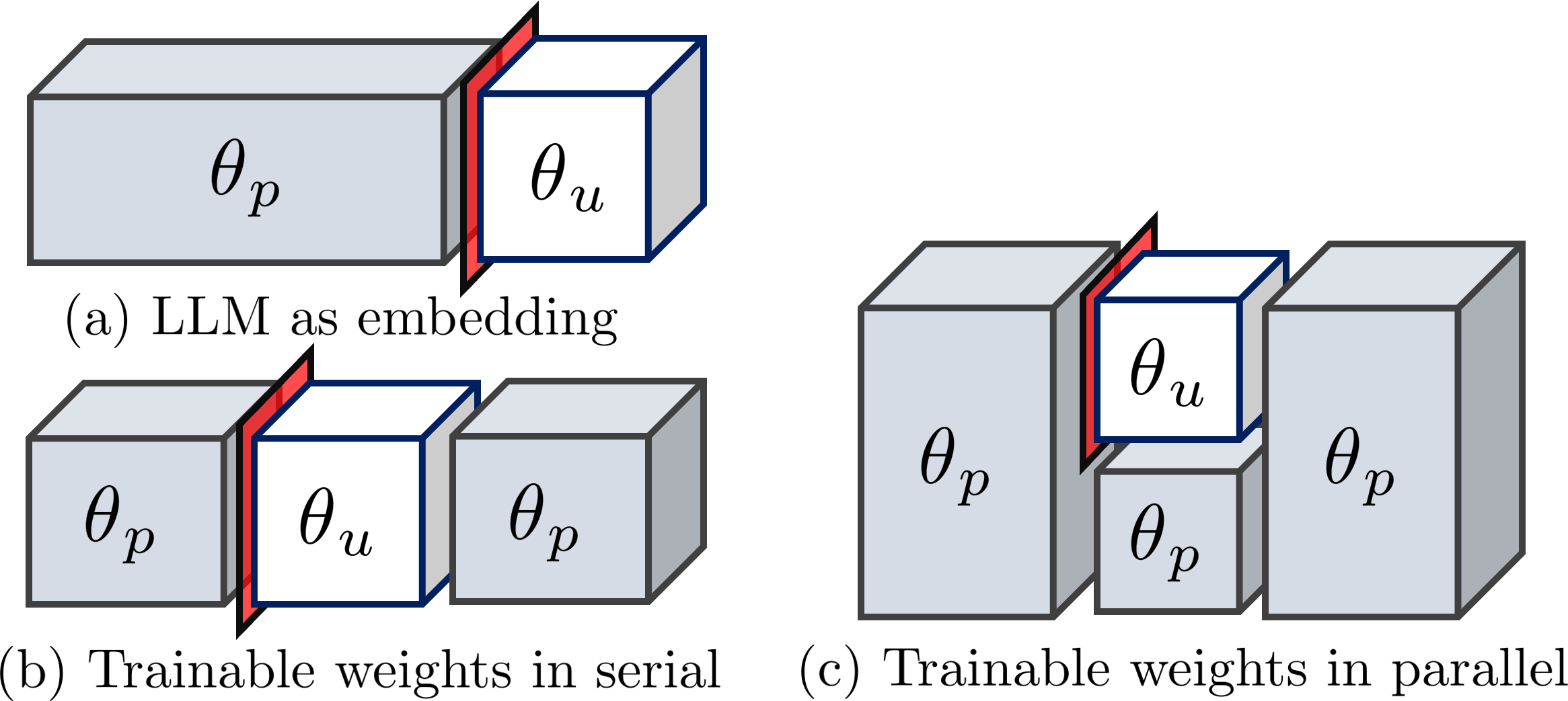
Figure 3: Different scenarios in training/fine-tuning LLMs in FL. The red squares show the privacy leakage surfaces in the threat model. The white and grey boxes indicate the trainable and frozen weights, respectively.

Fig.3 illustrates typical FL update scenarios with LLMs and their associated privacy leaking surfaces. The most common configuration (a) is when the LLM or some of its layers are used as embedding modules. In the second and third scenarios, additional modules with trainable weights are introduced sequentially (b) or in parallel (c). They capture the PET strategies involving adapters (Houlsby et al., 2019; Pfeiffer et al., 2020) and reparameterization tricks (Hu et al., 2022).

To make $\mathsf{Exp}^{\textup{AMI}}(\mathcal{A})$ describe the threats in Federated LLMs, the type of layers and weights in the trainable modules need to be specified. The assumption is that their inputs are hidden representations of the input data at some fixed locations of the language models. The most common layers are the fully connected (FC) layers and the attention mechanism (Vaswani et al., 2017). Consequently, our inference attacks are designed for those layers.

It is noteworthy to point out that, the actual pattern that the adversaries operate on is the embedded version of $T$, i.e., $\Phi_{\theta_{p}}(T)$. As the pre-trained parameters $\theta_{p}$ are public, and under a mild assumption that different target $T$ result in different embedding $\Phi_{\theta_{p}}(T)$, the problems of inferring $T$ and $\Phi_{\theta_{p}}(T)$ are equivalent . Therefore, in the subsequent discussions, we treat the embeddings as the user’s data for ease of notation.

4 ACTIVE MEMBERSHIP INFERENCE ATTACKS

This section presents our membership attacks and their theoretical guarantees in inferring data in FL on LLMs. The first attack, called FC-based adversary $\mathcal{A}_{\mathsf{FC}}$, is designed for scenarios where the first two trainable layers (See Fig. 3) are FC layers. The second attack, Attention-based adversary $\mathcal{A}_{\mathsf{Attn}}$, is tailored for cases when the first trainable layer is self-attention. The primary goal of both attacks is to create a neuron in those layers such that it is activated if and only if the target pattern is fed to the model. Consequently, the gradients of the weights computing that neuron are non-zero if and only if the target pattern is in the private training batch.

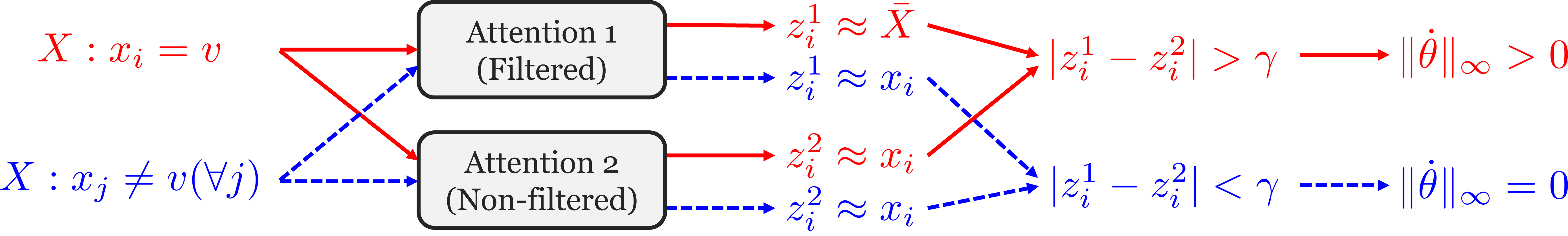
Figure 4: The $\mathcal{A}_{\mathsf{Attn}}$ adversary exploiting self-attention mechanism for membership inference in FL: If the target pattern $v=x_{i}$ is in the data, the output $z^{1}_{i}$ of the filtered head approximates the token’s average $\bar{X}$ instead of approximating $x_{i}$. This creates non-zero gradients for weights computing the difference between two heads.

4.1 FC-based adversary

The FC-based adversary $\mathcal{A}_{\mathsf{FC}}$ operates as follows. First, if the protocol permits, the initialization $\mathcal{A}_{\mathsf{FC-INIT}}$ specifies the model $\Phi$ in the FL training to use FC as its first two layers. For a target pattern $T$ with a dimension of $d_{T}$, the weights $W_{1}$ and biases $b_{1}$ of the first layer are set to dimensions $2d_{T}\times d_{T}$ and $2d_{T}$, respectively. If the protocol requires a larger dimension, extra parameters can be ignored. Conversely, if only smaller dimensions are allowed, the attacker uses a substring of $T$ as the detected pattern and proceeds from there. Since $\mathcal{A}_{\mathsf{FC}}$ uses only one output neuron at the second FC layer, the attack only needs to set one row and one entry of its weights and biases, denoted by $W_{2}[1,:]$ and $b_{2}[1]$. Particularly, the weights and biases of the two FC layers are set by $\mathcal{A}_{\mathsf{FC-ATTACK}}$ as:

$$W_{1}\leftarrow\begin{bmatrix}I_{d_{T}}\\ -I_{d_{T}}\end{bmatrix},\quad b_{1}\leftarrow\begin{bmatrix}-T\\ T\end{bmatrix}$$

$$W_{2}[1,:]\leftarrow-1_{d_{T}}^{\top},\quad b_{2}[1]\leftarrow\tau$$ (2)

where $I_{d_{T}}$ is the identity matrix and $1_{d_{T}}$ is the one-vector of size $d_{T}$. The parameter $\tau$ controls the allowable distance between an input $X$ and the target $T$, which can be obtained from the distribution statistics. In the guessing phase, $\mathcal{A}_{\mathsf{FC-GUESS}}$ returns $1$ if the gradient of $b_{2}[1]$ is non-zero and $0$ otherwise. Appx. A.1 provides a more detailed description of this attack.

Attack strategy. Upon receiving an input $X$, the two FC layers compute $z_{0}:=\max\left\{b_{2}[1]-\|X-T\|_{L_{1}},0\right\}$. If there is an $X=T$ in the data, $z_{0}$ will be activated and the gradient of the bias $b_{2}[1]$ is non-zero. On the other hand, for $b_{2}[1]=\tau>0$ small enough, $z_{0}=0$ for all $X\neq T$. Thus, the gradient of the bias $b_{2}[1]$ is zero when $T\notin D$. Therefore, the gradient of $b_{2}[1]$ indicates the presence of $T$ in the local data.

Remark 1.

The dimension of the target $T$. In practice, it is uncommon to feed the embedding of the entire input to FC layers. Instead, it is more common to forward each token individually. This means the target $T$ is the embedding of a token with a dimension of $d_{X}$. We might expect that this could hinder adversarial inference as a smaller portion of the input is exploited. However, as LLMs create strong connections among tokens, each token can embed the signature of the entire sentence. While this characteristic benefits the model’s performance, it also enables the inference of the input from the token level. Our experiments (Sect. 5) will consider both sentence embedding and token embedding and illustrate the above claim.

Attack advantage. The attack strategy implies that the adversary wins the security game $\mathsf{Exp}^{\textup{AMI}}$ with probability 1. We formalize that claim in Lemma 1:

Lemma 1.

The advantage of the adversary $\mathcal{A}_{\mathsf{FC}}$ in the security game $\mathsf{Exp}^{\textup{AMI}}$ is 1, i.e., ${\mathbf{\bf Adv}}^{\textup{AMI}}(\mathcal{A}_{\mathsf{FC}})=1$. (Proof in Appx. A.2)

Since $\mathcal{A}_{\mathsf{FC}}$ can be constructed in $\mathcal{O}(d_{T}^{2})$, the Lemma gives us the following theoretical result on the vulnerability of unprotected data in FL against AMI:

Theorem 1.

There exists an AMI adversary $\mathcal{A}$ exploiting 2 FC layers with time complexity $\mathcal{O}(d_{T}^{2})$ and advantage ${\mathbf{\bf Adv}}^{\textup{AMI}}(\mathcal{A})=1$ in the game $\mathsf{Exp}^{\textup{AMI}}$.

The implication of Theorem 1 is that unprotected private data of clients in FL is exposed to very high privacy risk, which was also observed by Nasr et al. (2019); Nguyen et al. (2023). However, the adversaries in those works involve multiple updates of either the FL model or other neural networks; thus, theoretical results on the trade-off between their success rates and complexities are not yet available. Therefore, it is unknown whether the vulnerability of Federated LLMs can be rigorously established from those attacks.

Remark 2.

Attack assumptions. The FC attack $\mathcal{A}_{\mathsf{FC}}$ does not need any distributional information to work on unprotected data. In fact, the attacker just needs to specify $\tau$ (2) small enough such that $\tau<\|X_{1}-X_{2}\|_{L_{1}}$ for any $X_{1}\neq X_{2}$ in the model’s dictionary. This is shown in the proof of Lemma 1 (Appx. A.2). Since the dictionary or the tokenizer is public, selecting $\tau$ does not require any additional information.

4.2 Attention-based adversary

Our proposed $\mathcal{A}_{\mathsf{Attn}}$ exploits the memorization capability of the self-attention, which was indirectly studied by Ramsauer et al. (2021). That work shows the attention is equivalent to the proposed Hopfield layer, whose main purpose is to directly integrate memorization into the layer. We adopt that viewpoint and introduce a specific configuration of the attention to make it memorize the local training data while filtering out the target of inference.

Since $\mathcal{A}_{\mathsf{Attn}}$ operates at a token level, the target of inference is the token resulting from embedding the target $T$, denoted by $v\in\mathbb{R}^{d_{X}}$. The intuition of $\mathcal{A}_{\mathsf{Attn}}$ is shown in Fig. 4: by setting an attention head to memorize the input batch and filter out the target token, $\mathcal{A}_{\mathsf{Attn}}$ introduces a gap between that head’s output and the output of a non-filtered head. The gap is then exploited to reveal the victim’s data. The following describes the components, strategy, and advantage of this attack.

Initialization $\mathcal{A}_{\mathsf{Attn-INIT}}$: The attack uses 4 attention heads, i.e., $H$ to 4. The layer dimensions are $d_{\textup{attn}}=d_{X}-1$, $d_{\textup{hid}}=d_{X}$ and $d_{Y}=2d_{X}$. Any configurations with more parameters can adopt this attack since the extra parameters can simply be ignored.

Hyper-parameters: $\beta,\gamma\in\mathbb{R}^{+}$

1 Randomly initialize $W_{Q}^{h},W_{K}^{h},W_{V}^{h},W_{O}$ and $b_{O}$ for all head $h\in\{1,2,3,4\}$

2Randomly initialize a matrix $W\in\mathbb{R}^{d_{X}\times d_{X}}$

3$W[:,1]\leftarrow v$ # Set the first column of $W$ to $v$

4$Q,R\leftarrow\textup{QR}(W)$ # QR-factorization $W$

5$W_{Q}^{1}\leftarrow Q[2:d_{X}]^{\top}$ # Embed pattern to $W_{Q}^{1}$

6$W_{K}^{1}\leftarrow\beta{{W_{Q}^{1}}^{\dagger\top}}$ # Set head $1$ to memorization

7$W_{K}^{2}\leftarrow\beta{{W_{Q}^{2}}^{\dagger\top}}$ # Set head $2$ to memorization

8$W_{Q}^{3}\leftarrow W_{Q}^{1}$, $W_{K}^{3}\leftarrow W_{K}^{1}$ # Copy head 1 to head 3

9$W_{Q}^{4}\leftarrow W_{Q}^{2}$, $W_{K}^{4}\leftarrow W_{K}^{2}$ # Copy head 2 to head 4

10$W_{V}^{1}\leftarrow I_{d_{X}}$, $W_{V}^{2}\leftarrow I_{d_{X}}$, $W_{V}^{3}\leftarrow I_{d_{X}}$, $W_{V}^{4}\leftarrow I_{d_{X}}$

11$W_{O}\leftarrow\begin{bmatrix}I_{d_{X}}&-I_{d_{X}}&0_{d_{X}}&0_{d_{X}}\\ 0_{d_{X}}&0_{d_{X}}&-I_{d_{X}}&I_{d_{X}}\end{bmatrix}$

12${b_{O}}_{i}=-\gamma,\forall i\in\{1,\cdots,d_{Y}\}$

13Ret all weights and biases

Algorithm 1 $\mathcal{A}_{\mathsf{Attn-ATTACK}}(v)$

Attack $\mathcal{A}_{\mathsf{Attn-ATTACK}}$: This step (Algo. 1) sets the attention weights $W_{Q}^{h},W_{K}^{h},W_{V}^{h},W_{O}$, and bias $b_{O}$, where $h$ is the head’s index. There are two hyper-parameters, $\beta$ and $\gamma\in\mathbb{R}^{+}$. While $\beta$ controls how much the heads memorize the input patterns $x_{i}^{h}$, $\gamma$ adjusts a cut-off thresholding between $v\in D$ and $v\notin D$ (Fig. 4). Given a target $v$, the first attention head is set such that:

$${W_{K}^{1\top}}W_{Q}^{1}\approx\beta I_{d_{X}}\quad\textup{and}\quad W_{Q}^{1}v\approx 0$$ (3)

To enforce (3), $d_{X}-1$ vectors orthogonal to $v\in\mathbb{R}^{d_{X}}$ are assigned to $W_{Q}^{1}$ via QR-factorization (line 1-1). Then, $W_{K}^{1}$ is set to the transpose of $\beta{{W_{Q}^{1\dagger}}}$, where $\dagger$ denotes the pseudo-inverse. On the other hand, the second head randomizes $W_{Q}^{2}$ and assigns $W_{K}^{2}$ as its pseudo-inverse. This means the second condition of (3) does not hold for the second head. The other parameters of the first two heads are set so that the first $d_{X}$ rows of $Y$ compute $\max\{0,Z^{1}-Z^{2}-\gamma 1^{\top}\}$. The third and the fourth heads are configured to compute the negations of the first two, i.e., they make the last $d_{X}$ rows of $Y$ return $\max\{0,Z^{2}-Z^{1}-\gamma 1^{\top}\}$. For ease of analysis, we construct $W_{V}^{h}$ and $W^{O}$ from identity and zero matrices.

Guessing $\mathcal{A}_{\mathsf{Attn-GUESS}}$: The attacker checks whether any of the weights in $W_{O}$ have non-zero gradients, and returns $b^{\prime}=1$ if that is the case.

Attack strategy. $\mathcal{A}_{\mathsf{Attn}}$ exploits the memorization imposed by the first condition of (3). To see how it works, we consider following the two cases:

Case 1: If $v\notin X$, $\nicefrac{{1}}{{\beta}}X^{\top}{W_{K}^{1\top}}W_{Q}^{1}X\approx X^{\top}X$, which is the correlation matrix of the tokens. The softmax’s output then approximates $I_{l_{X}}$ as the diagonal of $X^{\top}X$ is larger than other entries. The head’s output $Z^{1}\approx X$, i.e., $z^{1}_{i}\approx x_{i}$, as a result. Since the second head behaves similarly in this case, we have $Z^{2}\approx X$ and $z^{2}_{i}\approx x_{i}$.

Case 2: When $X$ contains $v$, the second condition of (3) makes $x_{i}^{\top}{W_{K}^{1\top}}W_{Q}^{1}x_{i}\approx 0$, and consequently causes the softmax’s output uniform, i.e., the attention is distributed equally among all tokens. Thus, the first head’s output is the token’s average $z^{1}_{i}\approx\bar{X}$. Since the second head does not filter $v$, $z^{2}_{i}\approx x_{i}$. The difference $|z^{1}_{i}-z^{2}_{i}|$ then reveals the presence of $v$ in $X$.

Attack advantage. The advantage of $\mathcal{A}_{\mathsf{Attn}}$ depends on an intrinsic measure of the data, called the Separation of Patterns (Ramsauer et al., 2021):

Definition 2.

(Separation of Patterns). For a token $x_{i}$ in $X=\{x_{j}\}_{j=1}^{l_{X}}$, its separation $\Delta_{i}$ from $X$ is $\Delta_{i}\coloneqq\min_{j,j\neq i}\left(x_{i}^{\top}x_{i}-x_{i}^{\top}{x}_{j}\right)=x_{i}^{\top}x_{i}-\max_{j}x_{i}^{\top}{x}_{j}$. We say $X$ is $\Delta$-separated if $\Delta_{i}\geq\Delta$ for all $i\in\{1,\cdots,l_{X}\}$. A data $D$ is $\Delta$-separated if all $X$ in $D$ are $\Delta$-separated.

Intuitively, $\Delta$-separated captures the intrinsic difficulty of adversarial inference on the data $D$: the less separating the data, i.e., a smaller $\Delta$, the harder to distinguish its tokens. In the context of LLMs, $\Delta$ is determined by the choice of the embedding modules. We are now ready for Lemma 2 about the advantage of $\mathcal{A}_{\mathsf{Attn}}$:

Lemma 2.

For a $\Delta$-separated data $D$ with i.i.d tokens of $\mathsf{Exp}^{\textup{AMI}}$, and for any $\beta>0$ large enough such that:

$$\Delta\geq{2}/{(\beta l_{X})}+\log(2(l_{X}-1)l_{X}\beta M^{2})/\beta$$ (4)

the advantage of $\mathcal{A}_{\mathsf{Attn}}$ satisfies:

$${\mathbf{\bf Adv}}^{\textup{AMI}}(\mathcal{A}_{\mathsf{Attn}})\geq P_{\textup{proj}}^{\mathcal{D}}\left(\frac{1}{\beta l_{X}M}\right)+$$

$$P_{\textup{proj}}^{\mathcal{D}}\left(\frac{1}{\beta l_{X}M}\right)^{2nl_{X}}-P_{\textup{box}}^{\mathcal{D}}(3\bar{\Delta})-1$$ (5)

where $\bar{\Delta}\coloneqq 2M(l_{X}-1)\exp\left(2/l_{X}-\beta\Delta\right)$. $P_{\textup{proj}}^{\mathcal{D}}(\delta)$ is the probability that the projected component between two independent tokens drawn from $\mathcal{D}$ is smaller than $\delta$ and $P_{\textup{box}}^{\mathcal{D}}(\delta)$ is the probability that a random token drawn from $\mathcal{D}$ is in the cube of size $2\delta$ centering at the mean of the tokens in $\mathcal{D}$. (Proof in Appx. B.1)

Table 1: General information of our experiments.

Experiment No. runs Adversary Dataset Language model Fig. 5 200 $\mathcal{A}_{\mathsf{Attn}}$ One-hot / Spherical / Gaussian No Fig. 6 $20\times 500$ $\mathcal{A}_{\mathsf{Attn}}$ IMDB BERT Table 2 $4\times 3\times 1\times 40$ $\mathcal{A}_{\mathsf{FC}}$ / $\mathcal{A}_{\mathsf{Attn}}$ / AMI (Nguyen et al., 2023) IMDB / Twitter / Yelp / Finance BERT / DistilBERT / RoBERTa / GPT1 / GPT2 Table 3 $4\times 3\times 4\times 10$ $\mathcal{A}_{\mathsf{FC}}$ / $\mathcal{A}_{\mathsf{Attn}}$ / AMI (Nguyen et al., 2023) IMDB / Twitter / Yelp / Finance BERT / DistilBERT / RoBERTa / GPT1 / GPT2 Table 4 $4\times 1\times 4\times 10$ $\mathcal{A}_{\mathsf{FC}}$ / $\mathcal{A}_{\mathsf{Attn}}$ IMDB / Twitter / Yelp / Finance BERT / DistilBERT / RoBERTa / GPT1 / GPT2

The key step of proving Lemma 2 is to rigorously show the configured attention layer operates as described in the attack strategy. We first bound the outputs $z_{i}^{h}$ of the layer when $x_{i}\neq v$ with Lemma 3 (Appx. B.1), which is a specific case of the Exponentially Small Retrieval Error Theorem (Ramsauer et al., 2021). The bound claims $z_{i}^{h}\approx x_{i}$ with a probability lower-bounded by $P_{\textup{proj}}^{\mathcal{D}}\left(\nicefrac{{1}}{{\beta l_{X}M}}\right)$. This controls the false-positive error. When $x_{i}=v$, $z^{1}_{i}\approx\bar{X}$ as described in the attack strategy. The false negatives happen when there exist other tokens filtered out unintentionally, i.e., they are near the center of the embedding. This probability is bounded by $P_{\textup{box}}^{\mathcal{D}}(3\bar{\Delta})$.

We now state some remarks about the advantage (5) on different embeddings and their asymptotic behaviors.

Remark 3.

$\Delta$ vs. the advantage (5). A larger $\Delta$ allows a smaller $\beta$ satisfied (4). It makes $P_{\textup{proj}}^{\mathcal{D}}\left(\nicefrac{{1}}{{\beta l_{X}M}}\right)$, and consequently, the lower bound (5) larger.

Remark 4.

Most vulnerable embedding. A data resulting in a lower bound (4) near 1 is one-hot data. Since it has no token alignment, $\Delta$ achieves its maximum and $P_{\textup{proj}}^{\mathcal{D}}\left(\nicefrac{{1}}{{\beta l_{X}M}}\right)$ is 1. Furthermore, since there is no token at the center of one-hot, a large $\beta$ can be selected so that $P_{\textup{box}}^{\mathcal{D}}(3\bar{\Delta})=0$ (See Fig. 5 for more).

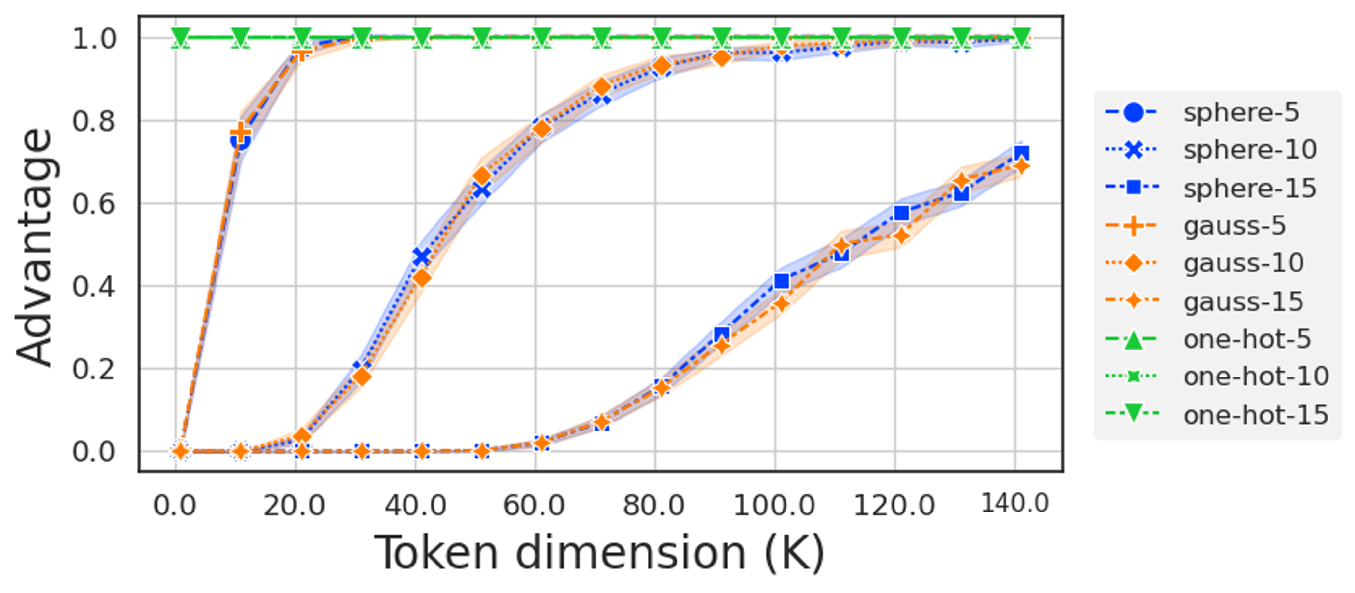
Figure 5: Simulations of the lower bound (5) for spherical, Gaussian and one-hot data with $l_{X}\in\{5,10,15\}$ (left). $\beta$ is chosen s.t. the ratios of $\Delta$ over the RHS of (4) $>1$, i.e., condition (4) holds (right).

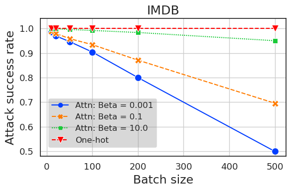
Figure 6: Success rates of $\mathcal{A}_{\mathsf{Attn}}$ on real-world IMDB dataset with different $\beta$.

Remark 5.

Asymptotic behavior of the advantage. For high dimensional data, i.e., large $d_{X}$, ${\mathbf{\bf Adv}}^{\textup{AMI}}(\mathcal{A})\rightarrow 1$. The reason is, when $d_{X}\rightarrow\infty$, two random points are surely almost orthogonal ($P_{\textup{proj}}^{\mathcal{D}}\rightarrow 1$), and a random point is almost always at the boundary ($P_{\textup{box}}^{\mathcal{D}}\rightarrow 0$) (Blum et al., 2020). Our Monte-Carlo simulations for the lower bound (5) for spherical, Gaussian, and one-hot data in Fig. 5 support that claim. It is clear that one-hot data results in an advantage of 1. Appx. B.2 provides more explanations for other data.

Table 2: Average Accuracies, F1, and AUCs of AMI attacks at different layers of LLMs on 4 real-world datasets. The methods are listed in decreasing order of trainable weights where $d_{x}=768,l_{x}\in\{24,32\}$ and $d_{h}=1000$ are the feature dimension, the number of tokens, and the method-specific parameter of the benchmark (Nguyen et al., 2023), respectively.

Method	No. params	BERT			RoBERTa			DistilBERT			GPT1			GPT2
		ACC	F1	AUC	ACC	F1	AUC	ACC	F1	AUC	ACC	F1	AUC	ACC	F1	AUC
$\mathcal{A}_{\mathsf{FC-Full}}$ (Ours)	$2l_{x}^{2}\times d_{x}^{2}$	1.00	1.00	1.00	1.00	1.00	1.00	1.00	1.00	1.00	1.00	1.00	1.00	1.00	1.00	1.00
AMI FC Full	$l_{x}\times d_{x}\times d_{h}$	0.94	0.95	0.94	0.78	0.74	0.78	0.87	0.88	0.88	1.00	1.00	1.00	0.78	0.78	0.83
$\mathcal{A}_{\mathsf{Attn}}$ (Ours)	$20d_{x}^{2}$	0.96	0.95	0.96	1.00	1.00	1.00	0.88	0.88	0.89	1.00	1.00	1.00	0.86	0.86	0.87
$\mathcal{A}_{\mathsf{FC-Token}}$ (Ours)	$2d_{x}^{2}$	1.00	1.00	1.00	1.00	1.00	1.00	1.00	1.00	1.00	1.00	1.00	1.00	1.00	1.00	1.00
AMI FC Token	$d_{x}\times d_{h}$	0.94	0.95	0.94	0.77	0.72	0.77	0.86	0.88	0.87	1.00	1.00	1.00	0.77	0.77	0.82

Table 3: Average Accuracies, F1, and AUCs of AMI attacks under DP defenses on 4 real-world datasets. The reported results are averaging among 4 DP mechanisms

$\varepsilon$-DP	Method	BERT			RoBERTa			DistilBERT			GPT1			GPT2
		ACC	F1	AUC	ACC	F1	AUC	ACC	F1	AUC	ACC	F1	AUC	ACC	F1	AUC
10	$\mathcal{A}_{\mathsf{FC-Full}}$ (Ours)	0.94	0.93	0.97	0.97	0.96	0.99	0.96	0.96	0.98	0.96	0.95	0.99	0.96	0.96	1.00
	AMI FC Full	0.68	0.68	0.69	0.67	0.66	0.67	0.68	0.69	0.70	0.62	0.62	0.65	0.66	0.65	0.67
	$\mathcal{A}_{\mathsf{Attn}}$ (Ours)	0.69	0.65	0.72	0.76	0.73	0.81	0.72	0.68	0.76	0.81	0.79	0.86	0.63	0.59	0.64
	$\mathcal{A}_{\mathsf{FC-Token}}$ (Ours)	0.87	0.85	0.92	0.90	0.89	0.93	0.90	0.90	0.96	0.91	0.89	0.94	0.91	0.90	0.94
	AMI FC Token	0.66	0.67	0.67	0.65	0.63	0.64	0.66	0.67	0.68	0.61	0.60	0.63	0.62	0.62	0.63
7.5	$\mathcal{A}_{\mathsf{FC-Full}}$ (Ours)	0.84	0.83	0.88	0.83	0.81	0.87	0.82	0.80	0.87	0.82	0.79	0.89	0.86	0.84	0.90
	AMI FC Full	0.57	0.56	0.58	0.58	0.58	0.58	0.62	0.61	0.62	0.52	0.51	0.54	0.58	0.59	0.59
	$\mathcal{A}_{\mathsf{Attn}}$ (Ours)	0.62	0.58	0.64	0.63	0.59	0.65	0.65	0.62	0.65	0.66	0.64	0.70	0.54	0.55	0.56
	$\mathcal{A}_{\mathsf{FC-Token}}$ (Ours)	0.72	0.68	0.77	0.76	0.73	0.82	0.76	0.74	0.81	0.69	0.65	0.73	0.76	0.74	0.80
	AMI FC Token	0.55	0.54	0.56	0.59	0.58	0.60	0.60	0.59	0.61	0.50	0.51	0.52	0.53	0.54	0.54
5	$\mathcal{A}_{\mathsf{FC-Full}}$ (Ours)	0.67	0.64	0.69	0.67	0.64	0.71	0.63	0.60	0.65	0.68	0.65	0.70	0.66	0.64	0.71
	AMI FC Full	0.55	0.54	0.56	0.53	0.54	0.53	0.54	0.52	0.55	0.53	0.51	0.53	0.55	0.56	0.56
	$\mathcal{A}_{\mathsf{Attn}}$ (Ours)	0.52	0.50	0.53	0.54	0.52	0.54	0.52	0.50	0.53	0.56	0.52	0.56	0.51	0.51	0.51
	$\mathcal{A}_{\mathsf{FC-Token}}$ (Ours)	0.57	0.53	0.60	0.60	0.58	0.63	0.59	0.58	0.61	0.58	0.53	0.59	0.57	0.55	0.59
	AMI FC Token	0.53	0.52	0.53	0.51	0.51	0.50	0.52	0.50	0.53	0.50	0.51	0.51	0.50	0.50	0.50

Remark 6.

Impact of $\beta$. A larger $\beta$ in $\mathcal{A}_{\mathsf{Attn}}$ increases the memorization of the attention (Ramsauer et al., 2021). We demonstrate its impact via an experiment of BERT (Devlin et al., 2019) and one-hot embeddings on the IMDB dataset. Fig. 6 shows that large $\beta$ can help $\mathcal{A}_{\mathsf{Attn}}$ make correct inferences even when the batch size is very large (500 sentences). One-hot embedding still achieves perfect inference regardless of the batch size as stated in Remark 4.

As $\mathcal{A}_{\mathsf{Attn}}$ can be constructed in $\mathcal{O}(d_{X}^{3})$, the Lemma gives us the theoretical vulnerability of unprotected data in FL with attention layer. We conclude this section with Theorem 2 about that claim.

Theorem 2.

There exists an adversary $\mathcal{A}$ exploiting a self-attention layer whose advantage satisfying (5) with time complexity $\mathcal{O}(d_{X}^{3})$ in the game $\mathsf{Exp}^{\textup{AMI}}$.

5 EXPERIMENTS

Table 4: Accuracies, F1, and AUCs at different layers ($\varepsilon=10$). We highlight the entries of the layers where the metrics achieve their highest values for each attack.

Layer	Method	RoBERTa			GPT1
		ACC	F1	AUC	ACC	F1	AUC
Early	$\mathcal{A}_{\mathsf{FC-Token}}$	0.88	0.87	0.92	0.93	0.93	0.97
	$\mathcal{A}_{\mathsf{Attn}}$	0.79	0.78	0.87	0.87	0.86	0.92
Mid	$\mathcal{A}_{\mathsf{FC-Token}}$	0.92	0.91	0.94	0.91	0.89	0.94
	$\mathcal{A}_{\mathsf{Attn}}$	0.80	0.77	0.86	0.83	0.80	0.91
Late	$\mathcal{A}_{\mathsf{FC-Token}}$	0.91	0.90	0.94	0.88	0.85	0.90
	$\mathcal{A}_{\mathsf{Attn}}$	0.68	0.65	0.71	0.73	0.71	0.75

This section provides experiments demonstrating the practical risks of leaking private data in FL with LLMs . In particular, we implement the FC-based $\mathcal{A}_{\mathsf{FC}}$ and self-attention-based $\mathcal{A}_{\mathsf{Attn}}$ adversaries and evaluate them in real-world setting. For the FC-based, we implement 2 versions, called $\mathcal{A}_{\mathsf{FC-Full}}$ and $\mathcal{A}_{\mathsf{FC-token}}$, which operate at a full sentence and at the token level (See Remark 1). For the benchmark, we extend the previous work (Nguyen et al., 2023) into two inference attacks also at sentence and token levels, called AMI FC Full and AMI FC Token, respectively.

Experimental Settings. Our attacks are evaluated on 5 state-of-the-art language models: BERT (Devlin et al., 2019), RoBERTa (Liu et al., 2019), distilBERT (Sanh et al., 2019), GPT1 (Brown et al., 2020), and GPT2 (Radford et al., 2019). The experiments are on 4 real-world text datasets: IMDB review (Maas et al., 2011), Yelp review (Zhang et al., 2015), Twitter-emotion (Saravia et al., 2018), and Finance (Casanueva et al., 2020). All models and datasets are from the Hugginingface database (Lhoest et al., 2021). Our experiment follows the security game in Fig. 2. The batch size $D$ is chosen to be 40. More information on the setting of our experiments is discussed in Appx. C.

To realize DP mechanisms, we use Generalized Randomized Response (GRR) (Dwork et al., 2006), Google RAPPOR (Erlingsson et al., 2014), Histogram encoding (HE) (Wang et al., 2017) and Microsoft dBitFlipPM (Ding et al., 2017) implemented by (Arcolezi et al., 2022). Table 1 provides the general information of our experiments. The No. runs indicates the total number of simulated security games for each point plotted/reported in our figures/tables. For instance, the expression $4\times 3\times 4\times 10$ means the results are averaged over 4 datasets, at 3 layers of the model, using 4 DP mechanisms and 10 security games. The reported privacy budget is applied once to the whole dataset and that budget is for a single communication round.

AMI without defense. Table 2 reports the average accuracies, F1 scores, and AUCs of attacks on all datasets at three locations of each model. The surfaces of attacks (Fig. 3) are the first, the middle, and the last layers (specified in more detail in Appx. C). The results are the averages among 4 datasets. Notably, FC-based attacks consistently achieve a $100\%$ success rate, aligning with the statement in Lemma 1. Furthermore, the attention-based attack exhibits competitive performance when compared to the benchmark (Nguyen et al., 2023). Note that, all of our methods have theoretical guarantees, and do not require neural network training. The table also includes the number of trainable weights in each attack. It serves as an indicator of the amount of fingerprints resulting from the attacks.

AMI with DP. We apply 4 DP mechanisms with budgets $\varepsilon\in\{5,7.5,10\}$ to evaluate the attacks in the high, medium, and low privacy regimes. Table 3 reports the results averaging from 4 mechanisms, 4 datasets, and 3 locations of each model. This gives us a general idea of how attacks perform under the presence of protected noise. Results for each defense are reported separately in Appx. D.

The first observation is that, at $\varepsilon=5$, almost all attacks fail to infer the pattern, i.e. AUCs $<0.72$; however, at mid and low privacy regimes, our attacks still achieve significant success rates. Especially, the FC-based $\mathcal{A}_{\mathsf{FC-Full}}$ and $\mathcal{A}_{\mathsf{FC-Token}}$ are always the top-2 with the highest performance. The results also show the advantages of $\mathcal{A}_{\mathsf{FC-Full}}$ over $\mathcal{A}_{\mathsf{FC-Token}}$ since it exploits all input information. On the other hand, both neural network approaches using AMI FC degrade rapidly with the presence of noise. Since they rely on over-fitting the target pattern, it becomes more challenging to successfully train the inference networks when the input dimension becomes large in the context of LLMs.

Inference at different layers. It is interesting to examine the privacy leakage at different locations of LLMs. We might expect that the deeper the attacking surface, the more private the data. However, we figured out that is not necessarily the case. Table 4 shows the performance of our attacks at different locations of RoBERTa and GPT1 at $\varepsilon=10$. While the claim holds for GPT1, it is not correct for RoBERTa. In fact, the layer with the highest success inference rates in RoBERTa is the mid-layer 6. Our hypothesis for the phenomenon is the tokens at that layer are more separated than those at the earlier layers. More results for other models are provided in Appx. D.

6 CONCLUSION

This work studies the formal threat models for AMI attacks with dishonest FL servers and demonstrates significant privacy threats in utilizing LLMs with FL for real-world applications. We provide evidence for the high success rates of active inference attacks, confirmed by both theoretical analysis and experimental evaluations. Our findings underscore the critical vulnerability of unprotected data in FL when confronted with dishonest servers. We extend our investigation to practical language models and gauge the privacy risks across different levels of DP budgets. Looking ahead, our future work will focus on identifying the prerequisites for a more secure centralized FL system and implementing these conditions effectively in practice. Furthermore, from a system perspective, we intend to explore decentralized FL protocols as a means to eliminate trust in a central server. We hope this work can serve as a stepping stone for future systematic updates and modifications of existing protocols, to make them more secure and robust for Federated LLMs.

Checklist

1. For all models and algorithms presented, check if you include:

   1. A clear description of the mathematical setting, assumptions, algorithm, and/or model. [Yes]

   2. An analysis of the properties and complexity (time, space, sample size) of any algorithm. [Yes]

   3. (Optional) Anonymized source code, with specification of all dependencies, including external libraries. [Yes]

2. For any theoretical claim, check if you include:

   1. Statements of the full set of assumptions of all theoretical results. [Yes]

   2. Complete proofs of all theoretical results. [Yes]

   3. Clear explanations of any assumptions. [Yes]

3. For all figures and tables that present empirical results, check if you include:

   1. The code, data, and instructions needed to reproduce the main experimental results (either in the supplemental material or as a URL). [Yes]

   2. All the training details (e.g., data splits, hyperparameters, how they were chosen). [Yes]

   3. A clear definition of the specific measure or statistics and error bars (e.g., with respect to the random seed after running experiments multiple times). [Yes, except for error statistics in the tables. The reason is the space limit.]

   4. A description of the computing infrastructure used. (e.g., type of GPUs, internal cluster, or cloud provider). [Yes]

4. If you are using existing assets (e.g., code, data, models) or curating/releasing new assets, check if you include:

   1. Citations of the creator If your work uses existing assets. [Yes]

   2. The license information of the assets, if applicable. [Yes]

   3. New assets either in the supplemental material or as a URL, if applicable. [Yes]

   4. Information about consent from data providers/curators. [Yes]

   5. Discussion of sensible content if applicable, e.g., personally identifiable information or offensive content. [Yes]

5. If you used crowdsourcing or conducted research with human subjects, check if you include:

   1. The full text of instructions given to participants and screenshots. [Not Applicable]

   2. Descriptions of potential participant risks, with links to Institutional Review Board (IRB) approvals if applicable. [Not Applicable]

   3. The estimated hourly wage paid to participants and the total amount spent on participant compensation. [Not Applicable]

 

APPENDIX

 

This is the appendix of our paper Analysis of Privacy Leakage in Federated Large Language Models. Its main content and outline are as follows:

• Appendix A shows more details of our results about the FC-based adversary in FL.

  • Appendix A.1: the description of our FC-based adversary for AMI.

  • Appendix A.2: the proof of Lemma 1.

• Appendix B shows more details of our results about the Attention-based adversary in FL.

  • Appendix B.1: the proof of Lemma 2.

  • Appendix B.2: the asymptotic behavior of the advantages of our self-attention-based adversary for spherical and Gaussian data.

• Appendix C provides the details of our experiments reported in the main manuscript.

  • Appendix C.1: details of the datasets.

  • Appendix C.2: details implementation of our adversaries.

• Appendix D provides additional experimental results.

Appendix A Vulnerability of FL to AMI Attack Exploiting FC Layers

This appendix reports the details of our theoretical results on AMI in FL. In Appx. A.1, we provide the descriptions of the proposed FC-based AMI adversary used in our analysis. Appx. A.2 shows the proof of Lemma 1.

A.1 FC-Based Adversary for AMI in FL

We now describe the FC-based adversary $\mathcal{A}_{\mathsf{FC}}$ mentioned in Sect. 4. The adversary is specified by the descriptions of its 3 components $\mathcal{A}_{\mathsf{FC-INIT}}$, $\mathcal{A}_{\mathsf{FC-ATTACK}}$ and $\mathcal{A}_{\mathsf{FC-GUESS}}$.

AMI initialization $\mathcal{A}_{\mathsf{FC-INIT}}$: The model specified by the adversary uses FC as its first two layers. Given an input $X\in\mathbb{R}^{d_{X}}$, the attacker computes $\textup{ReLU}(W_{l}X+b_{l})=\max(0,W_{l}X+b_{l})$ where $W_{l}$ is the weights and $b_{l}$ is the bias of layer $l$. We set the dimensions of $W_{1}$ and $b_{1}$ to $2d_{X}\times d_{X}$ and $2d_{X}$, respectively. For the second layer, the attack only considers one of its output neurons, thus, it only requires the number of columns of $W_{2}$ to be $2d_{X}$. We use $W_{2}[1,:]$ and $b_{2}[1]$ to refer to the parameters of the row of $W_{2}$ and the entry of $b_{2}$ corresponding to that neuron. Any configurations with a higher number of parameters can adopt our proposed attack because extra parameters can simply be ignored.

AMI attack $\mathcal{A}_{\mathsf{FC-ATTACK}}$: The weights and biases of the first two FC layers are set as:

$$W_{1}\leftarrow\begin{bmatrix}I_{d_{X}}\\ -I_{d_{X}}\end{bmatrix},\quad b_{1}\leftarrow\begin{bmatrix}-T\\ T\end{bmatrix},\quad W_{2}[1,:]\leftarrow-1_{d_{X}}^{\top},\quad b_{2}[1]\leftarrow\tau$$ (6)

where $I_{d_{X}}$ is the identity matrix and $1_{d_{X}}$ is the one vector of size $d_{X}$. The hyper-parameter $\tau$ controls the total allowable distance between an input $X$ and the target $T$, which can be obtained from the distribution statistics. The pseudo-code of the attack is shown in Algo. 2.

AMI guess $\mathcal{A}_{\mathsf{FC-GUESS}}$: In the guessing phase, the AMI server returns $1$ if the gradient of $b_{2}[1]$ is non-zero and returns $0$ otherwise. Algo. 3 shows the pseudo-code of this step.

Hyper-parameters: $\tau\in\mathbb{R}^{+}$

1

2 # Configuring $W_{1}\in\mathbb{R}^{2d_{X}\times d_{X}}$ and $b_{1}\in\mathbb{R}^{2d_{X}}$ of the first FC

3 $W_{1}\leftarrow\begin{bmatrix}I_{d_{X}}\\ -I_{d_{X}}\end{bmatrix},\quad b_{1}\leftarrow\begin{bmatrix}-T\\ T\end{bmatrix}$

4 # Configuring the first row of $W_{2}\in\mathbb{R}^{d\times 2d_{X}}$ and the first entry of $b_{2}\in\mathbb{R}^{d}$ of the second FC

5 $W_{2}[1,:]\leftarrow-1_{2d_{X}}^{\top},\quad b_{2}[1]\leftarrow\tau$

6Ret all weights and biases

Algorithm 2 $\mathcal{A}_{\mathsf{FC-ATTACK}}(T)$ exploiting fully-connected layer in AMI

1

2 # If the gradient of $b_{2}[1]$ is non-zero, returns $1$

3 if $|\dot{\theta}(b_{2}[1])|>0$ then

4       Ret $1$

5 end if

6Ret $0$

Algorithm 3 $\mathcal{A}_{\mathsf{FC-GUESS}}(T,\dot{\theta})$ exploiting fully-connected layer in AMI

A.2 Proof of Lemma 1 on the Advantage of the Adversary $\mathcal{A}_{\mathsf{FC}}$ in FL

This appendix provides the proof of Lemma 1. We restate the Lemma below:

Lemma.

The advantage of the adversary $\mathcal{A}_{\mathsf{FC}}$ in the security game $\mathsf{Exp}^{\textup{AMI}}$ is 1, i.e., ${\mathbf{\bf Adv}}^{\textup{AMI}}(\mathcal{A}_{\mathsf{FC}})=1$.

Proof.

For the model specified by $\mathcal{A}_{\mathsf{FC}}$ as discussed in Subsection 4.1, its first layer computes:

$$\textup{ReLU}\left(\begin{bmatrix}I_{d_{X}}\\ -I_{d_{X}}\end{bmatrix}X+\begin{bmatrix}-T\\ T\end{bmatrix}\right)=\textup{ReLU}\left(\begin{bmatrix}X-T\\ T-X\end{bmatrix}\right)$$ (7)

The first row of the second layer then computes:

$$z_{0}:= \textup{ReLU}\left(-\sum_{i=1}^{d_{X}}\textup{ReLU}\left(\left(x_{i}-t_{i}\right)+\textup{ReLU}\left(t_{i}-x_{i}\right)\right)+\tau\right)=\max\left\{\tau-\|X-T\|_{L_{1}},0\right\}$$ (8)

This implies the gradient of $b_{2}[1]=\tau$ is non-zero if and only if $\tau>\|X-T\|_{L_{1}}$. Thus, for a small enough $\tau$, $T\in D$ is equivalent to a non-zero gradient. Since $\dot{\theta}(b_{2}[1])$ is the average of gradients of $b_{2}[1]$ over $D$, we have:

$$\textup{If }b=0\Longrightarrow\ z_{0}=0,\forall X\in D\Longrightarrow\ |\dot{\theta}(b_{2}[1])|=0\Longrightarrow\ \mathcal{A}_{\mathsf{FC-GUESS}}\textup{ returns }0$$ (9)

$$\textup{If }b=1\Longrightarrow\ \left\{\begin{matrix}z_{0}>0\textup{ for }X=T\in D\\ z_{0}=0\textup{ for other }X\in D\end{matrix}\right.\Longrightarrow\ |\dot{\theta}(b_{2}[1])|>0\Longrightarrow\ \mathcal{A}_{\mathsf{FC-GUESS}}\textup{ returns }1$$ (10)

Thus, the advantage of $\mathcal{A}$ is $1$. ∎

Appendix B Vulnerability of FL to AMI Attack Exploiting Self-Attention Mechanism

This appendix provides the details of our theoretical results on exploiting the self-attention mechanism in FL. We show in Appx. B.1 the proof of Lemma 2 about the advantage of our proposed attention-based attack. We then discuss the asymptotic behavior of the advantages of $\mathcal{A}_{\mathsf{Attn}}$ for spherical and Gaussian data in Appendix B.2.

B.1 Proof of Lemma 2 on the Advantage of the Adversary $\mathcal{A}_{\mathsf{Attn}}$

We now state a Lemma bounding the error of the self-attention layer in memorization mode. The Lemma can be considered as a specific case of Theorem 5 of (Ramsauer et al., 2021). In the context of that work, they use the term for well-separated pattern in their main manuscript to indicate the condition that the Theorem holds. In fact, the condition (11) stated in our Lemma is a sufficient condition for that Theorem of (Ramsauer et al., 2021). For the completeness of this work, we now provide the highlight of the proof of Lemma 3 based on the theoretical results established in the work (Ramsauer et al., 2021).

Lemma 3.

Given a data $X$, a constant $\alpha>0$ large enough such that, for an $x_{i}\in X$:

$$\Delta_{i}\geq\frac{2}{\alpha l_{X}}+\frac{1}{\alpha}\log(2(l_{X}-1)l_{X}\alpha M^{2})$$ (11)

then, for any $\xi$ such that $\|\xi-x_{i}\|\leq\frac{1}{\alpha l_{X}M}$, we have

$$\left\|x_{i}-X\textup{softmax}\left(\alpha X^{\top}\xi\right)\right\|\leq 2M(l_{X}-1)\exp\left(2/l_{X}-\alpha\Delta_{i}\right)$$

Proof.

Define the sphere $S_{i}\coloneqq\{v\textup{ such that }\|v-x_{i}\|\leq 1/(\alpha l_{X}M)\}$. We now restate and apply some results of (Ramsauer et al., 2021):

For $\Delta_{i}$ satisfying (11) and a mapping $f_{\alpha}$ defined as $f_{\alpha}(\xi)=X\textup{softmax}\left(\alpha X^{\top}\xi\right)$, we have:

• The image of $S_{i}$ induced by $f_{\alpha}$ is in $S_{i}$, i.e., $f_{\alpha}$ is a mapping from $S_{i}$ to $S_{i}$ (Lemma A5 (Ramsauer et al., 2021)).

• $f_{\alpha}$ is a contraction mapping in $S_{i}$ (Lemma A6 (Ramsauer et al., 2021)).

• $f_{\alpha}$ has a fixed point in $S_{i}$ (Lemma A7 (Ramsauer et al., 2021)).

• Since $f_{\alpha}$ is a contraction mapping in $S_{i}$ and $\xi\in S_{i}$, we have

  $$\left\|x_{i}-f_{\alpha}(\xi)\right\|\leq 2M(l_{X}-1)\exp\left(-\alpha(\Delta_{i}-2\max\{\|\xi-x_{i}\|,\|x_{i}^{*}-x_{i}\|\}\right)$$

  where $x_{i}^{*}$ is a fixed point in $S_{i}$ (Theorem 5 (Ramsauer et al., 2021)).

Since both $x_{i}^{*}$ and $\xi$ are in $S_{i}$, we have $\max\{\|\xi-x_{i}\|,\|x_{i}^{*}-x_{i}\|\}\leq 1/(\alpha l_{X}M)$. Therefore, we obtain

$$\left\|x_{i}-f_{\alpha}(\xi)\right\|\leq 2M(l_{X}-1)\exp\left(-2/l_{X}-\alpha\Delta_{i}\right)$$

Thus, we have the Lemma. ∎

Intuitively, Lemma 3 claims that, if we have a pattern $\xi$ near $x_{i}$, $X\textup{softmax}\left(\alpha X^{\top}\xi\right)$ is exponentially near $\xi$ as a function of $\Delta_{i}$. Another key remark of the Lemma is that $\left\|x_{i}-X\textup{softmax}\left(\alpha X^{\top}\xi\right)\right\|$ exponentially approaches $0$ as the input dimension increases (Ramsauer et al., 2021).

We now prove Lemma 2 . We restate the Lemma below.

Lemma.

Given a $\Delta$-separated data $D$ with i.i.d tokens of the experiment $\mathsf{Exp}^{\textup{AMI}}$, for any $\beta>0$ large enough such that:

$$\Delta\geq{2}/{(\beta l_{X})}+\log(2(l_{X}-1)l_{X}\beta M^{2})/\beta$$

the advantage of $\mathcal{A}_{\mathsf{Attn}}$ satisfies:

$${\mathbf{\bf Adv}}^{\textup{AMI}}(\mathcal{A}_{\mathsf{Attn}})\geq P_{\textup{proj}}^{\mathcal{D}}\left(\frac{1}{\beta l_{X}M}\right)+P_{\textup{proj}}^{\mathcal{D}}\left(\frac{1}{\beta l_{X}M}\right)^{2nl_{X}}-P_{\textup{box}}^{\mathcal{D}}(3\bar{\Delta})-1$$

where $\bar{\Delta}\coloneqq 2M(l_{X}-1)\exp\left(2/l_{X}-\beta\Delta\right)$. $P_{\textup{proj}}^{\mathcal{D}}(\delta)$ is the probability that the projected component between two independent tokens drawn from $\mathcal{D}$ is smaller than $\delta$ and $P_{\textup{box}}^{\mathcal{D}}(\delta)$ is the probability that a random token drawn from $\mathcal{D}$ is in the cube of size $2\delta$ centering at the arithmetic mean of the tokens in $\mathcal{D}$.

Proof.

For brevity, we first consider the following expression and related notations of the output of one attention head without the head indexing $h$:

$$X\textup{softmax}\left(1/\sqrt{{d_{\textup{attn}}}}X^{\top}{W_{K}}^{\top}W_{Q}X\right)$$ (12)

Notice that we omit $W_{V}$ because they are all set to identity.

We now consider the AMI adversary $\mathcal{A}_{\mathsf{Attn}}$ specified in Subsection 4.2. As $W\in\mathbb{R}^{d_{X}\times d_{X}}$ (line 1 Algo. 1) is initiated randomly, it has a high probability to be non-singular even with the assignment of $v$ onto its first column (line 1 Algo. 1). For ease of analysis, we assume $W$ has full rank. If that is not the case, we can simply re-run those 2 lines of the algorithm. For the same arguments, we also assume all $W_{Q}^{h}$ and $W_{K}^{h}$ have rank ${d_{\textup{attn}}}=d_{X}-1$.

For all heads, we have $W_{K}=\beta(W_{Q}^{\top})^{\dagger}$ (lines 1 and 1 Algo. 1). As a consequence, $\frac{1}{\beta}W_{K}^{\top}W_{Q}=W_{Q}^{\dagger}W_{Q}$ is the projection matrix onto the column space of $W_{Q}^{\top}$. By denoting $[\xi_{1},\cdots,\xi_{l_{x}}]=\Xi=\frac{1}{\beta}{W_{K}}^{\top}W_{Q}X$, we have $\xi_{j}$ is the projection of the token $x_{j}$ onto that space.

For head 1 and head 3, due to line 1, we can write $W=[v,w_{2},\cdots,w_{d_{X}}]$. From the QR factorization (line 1), we have:

$$QR=[v,w_{2},\cdots w_{d_{X}}]\longrightarrow R=Q^{\top}[v,w_{2},\cdots w_{d_{X}}]$$

Since $R$ is an upper triangular matrix, $v$ is orthogonal to all rows $Q_{i},i\in\{2,\cdots,d_{X}\}$ of $Q^{\top}$. Furthermore, by the assignment at line 1, we have the column space of $W_{Q}^{\top}$ is the linear span of $\{Q_{i}\}_{i=2}^{d_{X}}$, which are all orthogonal to $v$. Consequently, the difference between $X$ and $\Xi$ is the component of $X$ along the $v$ direction:

$$X-\Xi^{h}=[x_{1}-\xi^{h}_{1},\cdots,x_{l_{X}}-\xi^{h}_{l_{X}}]=[\bar{x}^{v}_{1},\cdots,\bar{x}^{v}_{l_{X}}],\quad h\in\{1,3\}$$ (13)

where $\bar{x}^{v}_{j}$ is the component of token $x_{j}\in\mathbb{R}^{d_{X}}$ along $v$.

For head 2 and head 4, even though we do not conduct the QR-factorization, $\frac{1}{\beta}W_{K}^{\top}W_{Q}$ of those heads are also project matrices, just on different column space. These spaces are also of rank $d_{X}-1$ and it omits one direction. By calling that direction $u$, we can write the difference between $X$ and $\Xi$ for those heads as:

$$X-\Xi^{h}=[x_{1}-\xi^{h}_{1},\cdots,x_{l_{X}}-\xi^{h}_{l_{X}}]=[\bar{x}^{u}_{1},\cdots,\bar{x}^{u}_{l_{X}}],\quad h\in\{2,4\}$$ (14)

We now denote $f_{\alpha}:\mathbb{R}^{d_{X}\times l_{x}}\rightarrow\mathbb{R}^{d_{X}\times l_{x}}$ as:

$$\Xi^{\prime}=f_{\alpha}(\Xi)=X\textup{softmax}\left(\alpha X^{\top}\Xi\right)$$

For brevity, we also abuse the notation and write $\xi^{\prime}=f_{\alpha}(\xi)=X\textup{softmax}\left(\alpha X^{\top}\xi\right)$ for $\xi$ and $\xi^{\prime}\in\mathbb{R}^{d_{X}}$.

With that, the output of the layer before ReLU can be written as:

$$Z= \begin{bmatrix}f_{\beta}(\Xi^{1})-f_{\beta}(\Xi^{2})-\gamma 1^{\top}\\ f_{\beta}(\Xi^{4})-f_{\beta}(\Xi^{3})-\gamma 1^{\top}\end{bmatrix}=\begin{bmatrix}f_{\beta}(\Xi^{1})-f_{\beta}(\Xi^{2})-\gamma 1^{\top}\\ f_{\beta}(\Xi^{2})-f_{\beta}(\Xi^{1})-\gamma 1^{\top}\end{bmatrix}$$

$$= \begin{bmatrix}f_{\beta}(\xi_{1}^{1})-f_{\beta}(\xi_{1}^{2})-\gamma,&\cdots,&f_{\beta}(\xi_{l_{X}}^{1})-f_{\beta}(\xi_{l_{X}}^{2})-\gamma\\ f_{\beta}(\xi_{1}^{2})-f_{\beta}(\xi_{1}^{1})-\gamma,&\cdots,&f_{\beta}(\xi_{l_{X}}^{2})-f_{\beta}(\xi_{l_{X}}^{1})-\gamma\end{bmatrix}$$

where $\gamma$ is as given in Algo. 1 while $\beta$ is rescaled with a factor of $1/\sqrt{{d_{\textup{attn}}}}$. With the above expressions, we can see that $Z$ has non-zero entries if and only if:

$$\exists i\textup{ such that }\|f_{\beta}(\xi^{1}_{i})-f_{\beta}(\xi^{2}_{i})\|_{\infty}>\gamma$$ (15)

Note that the usage of heads 3 and 4 is for the entries of $f_{\beta}(\xi^{1}_{i})$ that are smaller than those in $f_{\beta}(\xi^{2}_{i})$. The condition (15) can also be expressed as

$$\|f_{\beta}(\Xi^{1})-f_{\beta}(\Xi^{2})\|_{\infty}>\gamma$$

For a given token $x_{i}$, we now consider two cases: $x_{i}\neq v$ and $x_{i}=v$.

Case 1. For a token $x_{i}\in X$ such that $x_{i}\neq v$, from Lemma 3, we have:

$$\left\|x_{i}-f_{\beta}(\xi^{1}_{i})\right\| \leq 2M(l_{X}-1)\exp\left(2/l_{X}-\beta\Delta_{i}\right)$$

$$\left\|x_{i}-f_{\beta}(\xi^{2}_{i})\right\| \leq 2M(l_{X}-1)\exp\left(2/l_{X}-\beta\Delta_{i}\right)$$

when $\|x_{i}-\xi^{1}_{i}\|=\|\bar{x}^{v}_{i}\|\leq 1/(\beta l_{X}M)$ and $\|\bar{x}^{u}_{i}\|\leq 1/(\beta l_{X}M)$, respectively. Note that we need to choose a $\beta$ large enough for the Lemma to hold. We denote those events by $A_{i}^{1}$ and $A_{i}^{2}$. Thus, from the triangle inequality, we have:

$$\|f_{\beta}(\xi^{1}_{i})-f_{\beta}(\xi^{2}_{i})\|\leq \left\|f_{\beta}(\xi^{1}_{i})-x_{i}\right\|+\left\|x_{i}-f_{\beta}(\xi^{2}_{i})\right\|\leq 4M(l_{X}-1)\exp\left(2/l_{X}-\beta\Delta_{i}\right)\coloneqq 2\bar{\Delta}_{i}$$

with probability of $\Pr\left[A_{i}^{1}\cap A_{i}^{2}\right]$. Here, we denote $\bar{\Delta}_{i}\coloneqq 2M(l_{X}-1)\exp\left(2/l_{X}-\beta\Delta_{i}\right)$. We further loosen the inequality with the infinity-norm, which bounds the maximum absolute difference in the pattern’s feature:

$$\|f_{\beta}(\xi^{1}_{i})-f_{\beta}(\xi^{2}_{i})\|_{\infty}\leq 2\bar{\Delta}_{i}$$

Since the data point $X$ is $\Delta$-separated, i.e., $\Delta\leq\Delta_{i}$, we further have:

$$\|f_{\beta}(\xi^{1}_{i})-f_{\beta}(\xi^{2}_{i})\|_{\infty}\leq 2\bar{\Delta}$$

where $\bar{\Delta}\coloneqq 2M(l_{X}-1)\exp\left(2/l_{X}-\beta\Delta\right)$.

We now consider the event $A^{1}_{i}$. Basically, that is the event the component of $x_{i}$ along $v$ is smaller than a constant determined by the data distribution $\mathcal{D}$. Furthermore, since both $v$ and $x_{i}$ are drawn independently from the distribution (specified in the experiment $\mathsf{Exp}^{\textup{AMI}}_{\textsc{None}}$), they can be considered as two random patterns drawn from the input distribution. Thus, the probability of $A^{i}_{1}$ is the probability that the projected component between two random tokens is smaller or equal to $\frac{1}{\beta l_{X}M}$. Formally, given an input distribution $\mathcal{D}$, we denote $P_{\textup{proj}}^{\mathcal{D}}(\delta)$ the probability that the projected component between any independent patterns drawn from $\mathcal{D}$ is less than or equal to $\delta$. We then have:

$$\Pr\left[A_{i}^{1}\right]=P_{\textup{proj}}^{\mathcal{D}}\left(\frac{1}{\beta l_{X}M}\right)$$

by definition. Similarly, for $A_{i}^{2}$, we have:

$$\Pr\left[A_{i}^{2}\right]=\Pr\left[\|\bar{x}^{u}_{i}\|\leq 1/(\beta l_{X}M)\right]=P_{\textup{proj}}^{\mathcal{D}}\left(\frac{1}{\beta l_{X}M}\right)$$

Since $v$ and $u$ are independent, we obtain:

$$\Pr\left[A_{i}^{1}\cap A_{i}^{2}\right]\geq P_{\textup{proj}}^{\mathcal{D}}\left(\frac{1}{\beta l_{X}M}\right)^{2}$$

Case 2. Since $v$ is orthogonal to all $\{Q_{i}\}_{i=2}^{d_{X}}$ for the matrix $Q$ at line 1, $W_{Q}v=0$ and, therefore, $\xi_{i}=0$. Consequently, if $x_{i}=v$, the output of the softmax is the one-vector scaled with a factor of $1/l_{X}$. We then have:

$$f_{\beta}(\xi_{i})=X\textup{softmax}(0)=\frac{1}{l_{X}}\sum_{j=1}^{l_{X}}x_{j}\coloneqq\bar{X}$$

Since $x_{i}=v$, we then obtain:

$$f_{\beta}(\xi^{1}_{i})-f_{\beta}(\xi^{2}_{i})=\bar{X}-f_{\beta}(\xi^{2}_{i})=\left(\bar{X}-v\right)+\left(x_{i}-f_{\beta}(\xi^{2}_{i})\right)$$

Thus, from triangle inequality, we have:

$$\left\|f_{\beta}(\xi^{1}_{i})-f_{\beta}(\xi^{2}_{i})\right\|_{\infty}\geq\left\|\bar{X}-v\right\|_{\infty}-\left\|x_{i}-f_{\beta}(\xi^{2}_{i})\right\|_{\infty}$$ (16)

$$\geq \left\|\bar{X}-v\right\|_{\infty}-\bar{\Delta}_{i}\geq\left\|\bar{X}-v\right\|_{\infty}-\bar{\Delta}$$ (17)

when $A^{2}_{i}$ happens, whose probability is $P_{\textup{proj}}^{\mathcal{D}}\left(\frac{1}{\beta l_{X}M}\right)$. We now consider the probability that $\left\|f_{\beta}(\xi^{1}_{i})-f_{\beta}(\xi^{2}_{i})\right\|_{\infty}>2\bar{\Delta}$:

$$\Pr\left[\left\|f_{\beta}(\xi^{1}_{i})-f_{\beta}(\xi^{2}_{i})\right\|_{\infty}>2\bar{\Delta}\right]$$ (18)

$$= 1-\Pr\left[\left\|f_{\beta}(\xi^{1}_{i})-f_{\beta}(\xi^{2}_{i})\right\|_{\infty}\leq 2\bar{\Delta}\right]$$ (19)

$$= 1-\Pr\left[\left\|f_{\beta}(\xi^{1}_{i})-f_{\beta}(\xi^{2}_{i})\right\|_{\infty}\leq 2\bar{\Delta}|A_{i}^{2}\right]\Pr\left[A_{i}^{2}\right]$$

$$- \Pr\left[\left\|f_{\beta}(\xi^{1}_{i})-f_{\beta}(\xi^{2}_{i})\right\|_{\infty}\leq 2\bar{\Delta}|\neg A_{i}^{2}\right]\Pr\left[\neg A_{i}^{2}\right]$$ (20)

$$\geq 1-\Pr\left[\left\|f_{\beta}(\xi^{1}_{i})-f_{\beta}(\xi^{2}_{i})\right\|_{\infty}\leq 2\bar{\Delta}|A_{i}^{2}\right]-\Pr\left[\neg A_{i}^{2}\right]$$ (21)

$$\geq 1-\Pr\left[\left\|\bar{X}-v\right\|_{\infty}-\bar{\Delta}\leq 2\bar{\Delta}|A_{i}^{2}\right]-\Pr\left[\neg A_{i}^{2}\right]$$ (22)

$$= 1-\Pr\left[\left\|\bar{X}-v\right\|_{\infty}\leq 3\bar{\Delta}\right]-\Pr\left[\neg A_{i}^{2}\right]$$ (23)

$$= P_{\textup{proj}}^{\mathcal{D}}\left(\frac{1}{\beta l_{X}M}\right)-\Pr\left[v\in\textup{Box}(\bar{X},3\bar{\Delta})\right]$$ (24)

where $\textup{Box}(x,\delta)$ is the cube of size $2\delta$ centering at $x$. The inequality (22) is due to (17) and (23) is from the fact that $u$ is independent from $X$ and $v$.

We now consider $\Pr\left[v\in\textup{Box}(\bar{X},3\bar{\Delta})\right]$, which is the probability that the pattern $v$ belongs to the cube of size $6\bar{\Delta}$ around the sampled mean of the tokens in $X$. We denote $P_{\textup{box}}^{\mathcal{D}}(\delta)$ the probability that a random pattern drawn from $\mathcal{D}$ is in the cube of size $2\delta$ centering at the arithmetic mean of the tokens in $\mathcal{D}$. If the length $l_{X}$ of $X$ is large enough, we have the sampled mean $\bar{X}$ is near the arithmetic mean of the tokens and obtain $\Pr\left[v\in\textup{Box}(\bar{X},3\bar{\Delta})\right]\approx P_{\textup{box}}^{\mathcal{D}}(3\bar{\Delta})$.

Back to main analysis. From the analysis of the two cases, if $v\notin X$, we have:

$$\Pr\left[\|f_{\beta}(\xi^{1}_{i})-f_{\beta}(\xi^{2}_{i})\|_{\infty}\leq 2\bar{\Delta}\right]\geq P_{\textup{proj}}^{\mathcal{D}}\left(\frac{1}{\beta l_{X}M}\right)^{2},\quad\forall i\in\{1,\cdots,l_{X}\}$$

If the tokens are independent, we then have:

$$\Pr\left[\|f_{\beta}(\Xi^{1})-f_{\beta}(\Xi^{2})\|_{\infty}\leq 2\bar{\Delta}\right]=\prod_{i=1}^{l_{X}}\Pr\left[\|f_{\beta}(\xi^{1}_{i})-f_{\beta}(\xi^{2}_{i})\|_{\infty}\leq 2\bar{\Delta}\right]\geq P_{\textup{proj}}^{\mathcal{D}}\left(\frac{1}{\beta l_{X}M}\right)^{2l_{X}}$$

Since the data points of $D$ are sampled independently, if $v$ does not appear in $D$, we then have:

$$\Pr\left[\|f_{\beta}(\Xi^{1})-f_{\beta}(\Xi^{2})\|_{\infty}\leq 2\bar{\Delta}\ \textup{ for all }X\in D\right]\geq P_{\textup{proj}}^{\mathcal{D}}\left(\frac{1}{\beta l_{X}M}\right)^{2nl_{X}}$$

On the other hand, if $v\in X$, we have:

$$\exists i\in\{1,\cdots,l_{X}\}\textup{ such that }\Pr\left[\|f_{\beta}(\xi^{1}_{i})-f_{\beta}(\xi^{2}_{i})\|_{\infty}>2\bar{\Delta}\right]\geq 1-P_{\textup{box}}^{\mathcal{D}}(3\bar{\Delta})$$

$$\Rightarrow \Pr\left[\|f_{\beta}(\Xi^{1})-f_{\beta}(\Xi^{2})\|_{\infty}>2\bar{\Delta}\right]\geq P_{\textup{proj}}^{\mathcal{D}}\left(\frac{1}{\beta l_{X}M}\right)-P_{\textup{box}}^{\mathcal{D}}(3\bar{\Delta})$$

Thus, if pattern $v$ appears in $D$, we have:

$$\Pr\left[\exists X\in D\textup{ such that }\|f_{\beta}(\Xi^{1})-f_{\beta}(\Xi^{2})\|_{\infty}>2\bar{\Delta}\right]\geq P_{\textup{proj}}^{\mathcal{D}}\left(\frac{1}{\beta l_{X}M}\right)-P_{\textup{box}}^{\mathcal{D}}(3\bar{\Delta})$$

By choosing $\gamma=2\bar{\Delta}$, we have the probability that our proposed adversary wins is:

$$P_{W}= \Pr\left[v\in D\right]\Pr\left[\|\dot{\theta}_{1}(W^{O})\|_{\infty}>0|v\in D\right]+\Pr\left[v\notin D\right]\Pr\left[\|\dot{\theta}_{1}(W^{O})\|_{\infty}=0|v\notin D\right]$$ (25)

$$= \frac{1}{2}\Pr\left[\exists X\in D\textup{ such that }\|f_{\beta}(\Xi^{1})-f_{\beta}(\Xi^{2})\|_{\infty}>2\bar{\Delta}|v\in D\right]$$

$$+ \frac{1}{2}\Pr\left[\|f_{\beta}(\Xi^{1})-f_{\beta}(\Xi^{2})\|_{\infty}\leq 2\bar{\Delta}\ \textup{ for all }X\in D|v\notin D\right]$$ (26)

$$\geq \frac{1}{2}\left(P_{\textup{proj}}^{\mathcal{D}}\left(\frac{1}{\beta l_{X}M}\right)-P_{\textup{box}}^{\mathcal{D}}(3\bar{\Delta})\right)+\frac{1}{2}P_{\textup{proj}}^{\mathcal{D}}\left(\frac{1}{\beta l_{X}M}\right)^{2nl_{X}}$$ (27)

Thus, the advantage of the adversary $\mathcal{A}_{\mathsf{Atnn}}$ in Algo. 1 can be bounded by:

$${\mathbf{\bf Adv}}^{\textup{AMI}}(\mathcal{A}_{\mathsf{Atnn}})=2P_{W}-1\geq P_{\textup{proj}}^{\mathcal{D}}\left(\frac{1}{\beta l_{X}M}\right)+P_{\textup{proj}}^{\mathcal{D}}\left(\frac{1}{\beta l_{X}M}\right)^{2nl_{X}}-P_{\textup{box}}^{\mathcal{D}}(3\bar{\Delta})-1$$ (28)

B.2 ${\mathbf{\bf Adv}}^{\textup{AMI}}(\mathcal{A}_{\mathsf{Atnn}})$ Approaches 1 for Spherical and Gaussian Data

This appendix provides the mathematical explanations for the asymptotic behaviors of the advantages ${\mathbf{\bf Adv}}^{\textup{AMI}}(\mathcal{A}_{\mathsf{Atnn}})$ for spherical and Gaussian data (Fig. 5).

Spherical data. We now consider the tokens are uniformly distributed on a unit sphere, i.e., $\|v\|=M=1$ for all $v$. We now argue that, when $\beta$ is large enough, we have the condition (4) of Lemma 2 and a small $\bar{\Delta}$ so that $P_{\textup{box}}^{\mathcal{D}}(3\bar{\Delta})=0$. For the projecting probability $P_{\textup{proj}}$, we have the distribution of the projected component between any pair of random tokens is the distribution of any one component of a random token. The reason is the choice of the second token does not matter and we can simply select it to be the standard vector $e_{i}$. Therefore, the expected value of the projected component between any pair of random tokens is $1/\sqrt{d_{X}}$. Thus, $P_{\textup{proj}}^{\mathcal{D}}\left(\frac{1}{\beta l_{X}M}\right)$ approaches 1 as $d_{X}$ increases. Consequentially, ${\mathbf{\bf Adv}}^{\textup{AMI}}(\mathcal{A}_{\mathsf{Atnn}})\rightarrow 1$ as $d_{X}$ increases.

Gaussian data. When the token in $X$ have standard normally distributed components, we have the expected value and the variance of the separation of two points are $d_{X}$ and $3d_{X}$, respectively (Ramsauer et al., 2021). We then assume that $\Delta>C_{1}d_{X}$ for some constant $C_{1}$. Since the expected norm of each token is $\sqrt{d_{X}}$, we further assume that $M\leq C_{2}\sqrt{d_{X}}$ for some constant $C_{2}$. With that, we can select $\beta=Kd_{X}^{-1}$ with $K$ large enough such that $\bar{\Delta}$ is small and the condition (4) holds. By that choice, we have $P_{\textup{box}}^{\mathcal{D}}(3\bar{\Delta})$ is the probability that all $l_{X}$ normal random variables are in $[-3\bar{\Delta},3\bar{\Delta}]$, which clearly approaches $0$ as $d_{X}$ increases. On the other hand, from the Central Limit Theorem, we have the dot product of two random tokens converge in distribution to a one-dimensional normal random variable, i.e., $u\cdot v/\sqrt{d_{X}}\rightarrow\mathcal{N}(0,1)$. Thus, as $d_{X}$ increases, we have $\Pr\left[\frac{|u\cdot v|}{\|v\|}<C_{3}\right]\rightarrow 1$ for a large enough constant $C_{3}$. As $\frac{1}{\beta l_{X}M}>\frac{\sqrt{d_{X}}}{Kl_{X}C_{2}}$, we have $P_{\textup{proj}}^{\mathcal{D}}\left(\frac{1}{\beta l_{X}M}\right)\rightarrow 1$.

∎

Appendix C Experimental Settings

This appendix provides the experimental details of our experiments. Our experiments are implemented using Python 3.8 and conducted on a single GPU-assisted compute node that is installed with a Linux 64-bit operating system. The allocated resources include 36 CPU cores with 2 threads per core and 60GB of RAM. The node is also equipped with 8 GPUs, with 80GB of memory per GPU.

We now provide more information on the tested dataset in Appx. C.1 and the details implementation of our adversaries in Appx. C.2.

C.1 Dataset and the Language Models

In total, our experiments are conducted on 3 synthetic datasets and 4 real-world datasets. The synthetic datasets are one-hot encoded data, Spherical data (data on the boundary of a unit ball), and Gaussian data (each dimension is an independent $\mathcal{N}(0,1)$). The real-world datasets are IMDB (movie reviews) (Maas et al., 2011), Yelp (general reviews) (Zhang et al., 2015), Twitter (Twitter messages with emotions) (Saravia et al., 2018), and Finance (meassage with intents) (Casanueva et al., 2020). The real-world datasets are pre-processed with the LLMs as embedding modules to obtain the data $D$ in our threat models. For the synthetic datasets, we use a batch size of $1$ since it does not affect the asymptotic behaviors and provides better intuition for the experiment of Fig. 5. For the real-world datasets, we use a batch size of 40.

Table 5: General information about the LLMs.

BERT RoBERTa DistilBERT GPT1 GPT2 No. params 110M 125M 67M 120M 137M No. layers 12 12 6 12 6 No. tokens ($l_{x}$) 32 32 32 32 32 Dimension ($d_{x}$) 768 768 768 768 768 Attacking layers 1,6,12 1,6,12 1,3,6 1,6,12 1,3,6

Table 5 provides information about the LLMs examined in our experiments. Their implementations are provided by the Huggingface library (Lhoest et al., 2021). The rows No. tokens and dimension refers to the number of tokens and the embedded dimension of the tokens. The dimension is 768 at all hidden layers of all language models. The Attacking layers are the layers that we conduct our inference attacks. They correspond to the early, middle, and late locations of attacking mentioned in Sect. 5 of the main manuscript.

C.2 Implementation of the Adversaries

In our theoretical analysis of $\mathcal{A}_{\mathsf{FC}}$ and $\mathcal{A}_{\mathsf{Attn}}$, we have specified how their hyper-parameters should be chosen so that theoretical guarantees can be achieved. For convenience reference, we restate those settings here:

• For Lemma 1, $\tau$ can be any small positive number such that $\tau<\|X-T\|_{L_{1}}$ for all $X\neq T$ in the dataset. In other words, we just need to choose a very small positive number. The argument is made at Subsect. 4.1.

• For Lemma 2, $\beta$ is chosen large enough such that the condition (4) of the Lemma holds and $\gamma$ is set to $2\bar{\Delta}$. The argument is made at (25) in Appx. B.1.

Table 6: Values of $\beta$ in the reported experiments.

Dataset Note on $\beta$ $\beta$ One-hot / Spherical $\beta$ is is set to a constant 10 Gaussian $\beta\propto 1/d_{X}$ $10/d_{X}$ Real-world data The more noise, the smaller $\beta$ 2

As stated in Remark 6 the parameter $\beta$ of our proposed attention-based adversary determines how much the input patterns are memorized. While increasing $\beta$ can increase the adversary’s success rate of inference, it decreases the attack’s performance when privacy-preserving noise is added to the data. The actual values of $\beta$ in our experiments are reported in Table 6.

Table 7: Average Accuracies, F1, and AUCs of AMI attacks under GRR defense (Dwork et al., 2006).

$\varepsilon$	Method	BERT			RoBERTa			DistilBERT			GPT1			GPT2
		ACC	F1	AUC	ACC	F1	AUC	ACC	F1	AUC	ACC	F1	AUC	ACC	F1	AUC
10	$\mathcal{A}_{\mathsf{FC-Full}}$	1.00	1.00	1.00	1.00	1.00	1.00	1.00	1.00	1.00	1.00	1.00	1.00	1.00	1.00	1.00
	$\mathcal{A}_{\mathsf{Attn}}$	0.89	0.88	0.92	0.99	0.99	1.00	0.82	0.80	0.82	1.00	1.00	1.00	0.84	0.82	0.85
	$\mathcal{A}_{\mathsf{FC-Token}}$	1.00	1.00	1.00	1.00	1.00	1.00	1.00	1.00	1.00	1.00	1.00	1.00	1.00	1.00	1.00
7.5	$\mathcal{A}_{\mathsf{FC-Full}}$	0.99	0.99	1.00	1.00	1.00	1.00	1.00	1.00	1.00	0.99	0.99	1.00	0.99	0.99	1.00
	$\mathcal{A}_{\mathsf{Attn}}$	0.77	0.74	0.82	0.94	0.93	0.99	0.82	0.82	0.85	0.93	0.93	0.99	0.70	0.67	0.75
	$\mathcal{A}_{\mathsf{FC-Token}}$	0.97	0.96	1.00	0.94	0.93	0.99	0.98	0.98	0.99	0.97	0.97	1.00	0.99	0.99	1.00
5	$\mathcal{A}_{\mathsf{FC-Full}}$	0.83	0.81	0.85	0.89	0.87	0.95	0.81	0.79	0.87	0.82	0.79	0.90	0.83	0.79	0.96
	$\mathcal{A}_{\mathsf{Attn}}$	0.56	0.51	0.60	0.67	0.62	0.69	0.61	0.52	0.64	0.64	0.60	0.67	0.50	0.50	0.50
	$\mathcal{A}_{\mathsf{FC-Token}}$	0.71	0.65	0.79	0.72	0.70	0.77	0.74	0.71	0.76	0.71	0.65	0.73	0.72	0.71	0.78

Table 8: Average Accuracies, F1, and AUCs of AMI attacks under RAPPOR defense (Erlingsson et al., 2014).

$\varepsilon$	Method	BERT			RoBERTa			DistilBERT			GPT1			GPT2
		ACC	F1	AUC	ACC	F1	AUC	ACC	F1	AUC	ACC	F1	AUC	ACC	F1	AUC
10	$\mathcal{A}_{\mathsf{FC-Full}}$	0.97	0.97	1.00	0.98	0.98	1.00	0.98	0.98	1.00	1.00	1.00	1.00	0.99	0.99	1.00
	$\mathcal{A}_{\mathsf{Attn}}$	0.63	0.59	0.69	0.73	0.70	0.81	0.71	0.67	0.74	0.80	0.77	0.89	0.55	0.50	0.54
	$\mathcal{A}_{\mathsf{FC-Token}}$	0.90	0.88	0.95	0.94	0.93	0.97	0.92	0.91	0.97	0.91	0.89	0.95	0.95	0.94	0.98
7.5	$\mathcal{A}_{\mathsf{FC-Full}}$	0.87	0.85	0.90	0.84	0.82	0.87	0.82	0.79	0.90	0.83	0.81	0.92	0.88	0.85	0.91
	$\mathcal{A}_{\mathsf{Attn}}$	0.60	0.56	0.63	0.55	0.52	0.57	0.61	0.58	0.60	0.57	0.53	0.60	0.50	0.50	0.50
	$\mathcal{A}_{\mathsf{FC-Token}}$	0.68	0.63	0.76	0.76	0.73	0.82	0.73	0.70	0.78	0.59	0.55	0.64	0.73	0.71	0.81
5	$\mathcal{A}_{\mathsf{FC-Full}}$	0.62	0.60	0.68	0.55	0.51	0.57	0.53	0.51	0.52	0.60	0.56	0.55	0.62	0.61	0.66
	$\mathcal{A}_{\mathsf{Attn}}$	0.50	0.50	0.50	0.50	0.50	0.50	0.50	0.50	0.50	0.50	0.50	0.50	0.50	0.50	0.50
	$\mathcal{A}_{\mathsf{FC-Token}}$	0.53	0.50	0.53	0.53	0.50	0.55	0.55	0.54	0.58	0.57	0.50	0.58	0.50	0.50	0.51

Table 9: Average Accuracies, F1, and AUCs of AMI attacks under THE defense (Wang et al., 2017).

$\varepsilon$	Method	BERT			RoBERTa			DistilBERT			GPT1			GPT2
		ACC	F1	AUC	ACC	F1	AUC	ACC	F1	AUC	ACC	F1	AUC	ACC	F1	AUC
10	$\mathcal{A}_{\mathsf{FC-Full}}$	0.80	0.77	0.89	0.90	0.88	0.97	0.87	0.84	0.92	0.86	0.83	0.96	0.89	0.88	0.98
	$\mathcal{A}_{\mathsf{Attn}}$	0.56	0.51	0.60	0.58	0.53	0.63	0.65	0.59	0.68	0.65	0.61	0.68	0.58	0.53	0.60
	$\mathcal{A}_{\mathsf{FC-Token}}$	0.70	0.65	0.78	0.75	0.72	0.80	0.76	0.74	0.86	0.77	0.73	0.84	0.73	0.72	0.78
7.5	$\mathcal{A}_{\mathsf{FC-Full}}$	0.67	0.63	0.74	0.61	0.57	0.64	0.62	0.58	0.61	0.62	0.57	0.73	0.71	0.68	0.77
	$\mathcal{A}_{\mathsf{Attn}}$	0.50	0.50	0.50	0.50	0.50	0.50	0.60	0.54	0.60	0.56	0.54	0.59	0.50	0.50	0.50
	$\mathcal{A}_{\mathsf{FC-Token}}$	0.58	0.53	0.61	0.60	0.55	0.65	0.59	0.57	0.66	0.59	0.53	0.63	0.60	0.59	0.63
5	$\mathcal{A}_{\mathsf{FC-Full}}$	0.58	0.55	0.59	0.57	0.55	0.62	0.61	0.57	0.67	0.67	0.63	0.74	0.57	0.54	0.60
	$\mathcal{A}_{\mathsf{Attn}}$	0.50	0.50	0.50	0.51	0.50	0.50	0.50	0.50	0.50	0.56	0.53	0.56	0.50	0.50	0.50
	$\mathcal{A}_{\mathsf{FC-Token}}$	0.52	0.49	0.56	0.54	0.54	0.56	0.50	0.50	0.51	0.51	0.50	0.50	0.53	0.53	0.50

Table 10: Average Accuracies, F1, and AUCs of AMI attacks under dBitFlipPM defense (Ding et al., 2017).

$\varepsilon$	Method	BERT			RoBERTa			DistilBERT			GPT1			GPT2
		ACC	F1	AUC	ACC	F1	AUC	ACC	F1	AUC	ACC	F1	AUC	ACC	F1	AUC
10	$\mathcal{A}_{\mathsf{FC-Full}}$	0.97	0.97	1.00	0.98	0.98	1.00	0.99	0.99	1.00	0.98	0.98	1.00	0.97	0.96	1.00
	$\mathcal{A}_{\mathsf{Attn}}$	0.66	0.64	0.67	0.73	0.71	0.81	0.72	0.68	0.79	0.80	0.79	0.86	0.57	0.54	0.59
	$\mathcal{A}_{\mathsf{FC-Token}}$	0.89	0.87	0.96	0.93	0.92	0.96	0.93	0.93	0.99	0.93	0.92	0.96	0.95	0.95	0.99
7.5	$\mathcal{A}_{\mathsf{FC-Full}}$	0.84	0.83	0.90	0.88	0.86	0.95	0.86	0.85	0.96	0.84	0.81	0.90	0.86	0.83	0.92
	$\mathcal{A}_{\mathsf{Attn}}$	0.59	0.55	0.61	0.55	0.51	0.55	0.57	0.53	0.56	0.59	0.57	0.62	0.51	0.51	0.51
	$\mathcal{A}_{\mathsf{FC-Token}}$	0.66	0.59	0.73	0.74	0.72	0.80	0.75	0.72	0.80	0.61	0.55	0.65	0.70	0.67	0.77
5	$\mathcal{A}_{\mathsf{FC-Full}}$	0.59	0.57	0.60	0.62	0.60	0.67	0.56	0.51	0.57	0.63	0.62	0.65	0.62	0.61	0.63
	$\mathcal{A}_{\mathsf{Attn}}$	0.55	0.50	0.57	0.51	0.50	0.52	0.50	0.50	0.50	0.55	0.50	0.54	0.50	0.50	0.50
	$\mathcal{A}_{\mathsf{FC-Token}}$	0.52	0.50	0.54	0.61	0.59	0.63	0.59	0.58	0.59	0.55	0.50	0.55	0.54	0.50	0.56

Appendix D More Experimental Results

Due to the length constraints, the main manuscript only provides the average results of different Differential Privacy (DP) mechanisms in Table 3. In the following, we present more detailed results for our proposed membership inference attacks under each DP mechanism separately.

Specifically, we display the accuracies, F1 scores, and AUCs of the attacks for four different DP mechanisms: Generalized Randomized Response (GRR)(Dwork et al., 2006) in Table7, Google RAPPOR (Erlingsson et al., 2014) in Table 8, Histogram encoding (HE)(Wang et al., 2017) in Table9, and Microsoft dBitFlipPM (Ding et al., 2017) in Table 10. The DP mechanisms are applied at the token’s index level using the Multi-Freq-LDPy library (Arcolezi et al., 2022). Despite all of these mechanisms providing the same theoretical DP guarantee, there are subtle differences in the performance of the defense methods.

It is unsurprising that GRR consistently yields the highest successful inference rates given its status as one of the pioneers in the field of DP. When considering the relative performance among the other mechanisms, no clear winner emerges as the outcomes vary depending on the attacking methods and the examined models.

It is also worth noting that GPT models appear to exhibit greater resilience against attention-based attacks when compared to BERT-based models. Our hypothesis is grounded in the distinctive architectural differences between the GPTs, which feature a ”decoder-only” design, and the BERTs, which employ an ”encoder-only” architecture.

Table 11: Accuracies, F1, and AUCs at different layers ($\varepsilon=10$).

Layer	Method	BERT			RoBERTa			DistilBERT			GPT1			GPT2
		ACC	F1	AUC	ACC	F1	AUC	ACC	F1	AUC	ACC	F1	AUC	ACC	F1	AUC
Early	$\mathcal{A}_{\mathsf{FC-Full}}$	0.98	0.98	1.00	0.99	0.99	1.00	0.99	0.99	1.00	0.98	0.97	1.00	0.98	0.98	1.00
	$\mathcal{A}_{\mathsf{Attn}}$	0.86	0.83	0.92	0.79	0.78	0.87	0.91	0.89	0.96	0.87	0.86	0.92	0.50	0.50	0.50
	$\mathcal{A}_{\mathsf{FC-Token}}$	0.88	0.87	0.94	0.88	0.87	0.92	0.91	0.90	0.96	0.93	0.93	0.97	0.89	0.89	0.92
Mid	$\mathcal{A}_{\mathsf{FC-Full}}$	0.97	0.97	1.00	0.96	0.96	1.00	0.96	0.96	1.00	0.96	0.96	1.00	0.96	0.95	1.00
	$\mathcal{A}_{\mathsf{Attn}}$	0.66	0.63	0.68	0.80	0.77	0.86	0.80	0.76	0.86	0.83	0.80	0.91	0.63	0.59	0.65
	$\mathcal{A}_{\mathsf{FC-Token}}$	0.93	0.92	0.96	0.92	0.91	0.94	0.90	0.89	0.95	0.91	0.89	0.94	0.91	0.89	0.94
Late	$\mathcal{A}_{\mathsf{FC-Full}}$	0.85	0.83	0.91	0.94	0.94	0.98	0.94	0.93	0.94	0.94	0.92	0.97	0.96	0.95	0.99
	$\mathcal{A}_{\mathsf{Attn}}$	0.54	0.50	0.55	0.68	0.65	0.71	0.50	0.50	0.50	0.73	0.71	0.75	0.67	0.61	0.68
	$\mathcal{A}_{\mathsf{FC-Token}}$	0.80	0.75	0.86	0.91	0.90	0.94	0.90	0.89	0.95	0.88	0.85	0.90	0.93	0.92	0.95

Table 11 reports the performance of our attacks at different locations of all five language models with $\varepsilon=10$. This table can be considered as the full version of Table 4 in our main manuscript. We can see that, in general, it is more challenging to infer the target data as the attacking surfaces get deeper. However, in BERT and RoBERTa, we observe a slight increase in the successful inference rates of $\mathcal{A}_{\mathsf{FC-Token}}$ around the middle layers of the models.

References

- Arcolezi et al. (2022) Héber H. Arcolezi, Jean-François Couchot, Sébastien Gambs, Catuscia Palamidessi, and Majid Zolfaghari. Multi-freq-LDPy: Multiple frequency estimation under local differential privacy in python. In Computer Security – ESORICS 2022, pages 770–775. Springer Nature Switzerland, 2022. doi: 10.1007/978-3-031-17143-7˙40. URL https://doi.org/10.1007/978-3-031-17143-7_40.
- Beaufays et al. (2019) Francoise Beaufays, Kanishka Rao, Rajiv Mathews, and Swaroop Ramaswamy. Federated learning for emoji prediction in a mobile keyboard, 2019. URL https://arxiv.org/abs/1906.04329.
- Ben Zaken et al. (2022) Elad Ben Zaken, Yoav Goldberg, and Shauli Ravfogel. BitFit: Simple parameter-efficient fine-tuning for transformer-based masked language-models. In Proceedings of the 60th Annual Meeting of the Association for Computational Linguistics (Volume 2: Short Papers), pages 1–9, Dublin, Ireland, May 2022. Association for Computational Linguistics. doi: 10.18653/v1/2022.acl-short.1. URL https://aclanthology.org/2022.acl-short.1.
- Blum et al. (2020) Avrim Blum, John Hopcroft, and Ravindran Kannan. Foundations of Data Science. Cambridge University Press, 2020. doi: 10.1017/9781108755528.
- Boenisch et al. (2021) Franziska Boenisch, Adam Dziedzic, Roei Schuster, Ali Shahin Shamsabadi, Ilia Shumailov, and Nicolas Papernot. When the curious abandon honesty: Federated learning is not private. arXiv preprint arXiv:2112.02918, 2021.
- Brown et al. (2020) Tom Brown, Benjamin Mann, Nick Ryder, Melanie Subbiah, Jared D Kaplan, Prafulla Dhariwal, Arvind Neelakantan, Pranav Shyam, Girish Sastry, Amanda Askell, Sandhini Agarwal, Ariel Herbert-Voss, Gretchen Krueger, Tom Henighan, Rewon Child, Aditya Ramesh, Daniel Ziegler, Jeffrey Wu, Clemens Winter, Chris Hesse, Mark Chen, Eric Sigler, Mateusz Litwin, Scott Gray, Benjamin Chess, Jack Clark, Christopher Berner, Sam McCandlish, Alec Radford, Ilya Sutskever, and Dario Amodei. Language models are few-shot learners. In H. Larochelle, M. Ranzato, R. Hadsell, M.F. Balcan, and H. Lin, editors, Advances in Neural Information Processing Systems, volume 33, pages 1877–1901. Curran Associates, Inc., 2020.
- Bui et al. (2019) Duc Bui, Kshitiz Malik, Jack Goetz, Honglei Liu, Seungwhan Moon, Anuj Kumar, and Kang G Shin. Federated user representation learning. arXiv preprint arXiv:1909.12535, 2019.
- Carlini et al. (2022) Nicholas Carlini, Steve Chien, Milad Nasr, Shuang Song, Andreas Terzis, and Florian Tramer. Membership inference attacks from first principles. In 2022 IEEE Symposium on Security and Privacy (SP), pages 1897–1914. IEEE, 2022.
- Casanueva et al. (2020) Iñigo Casanueva, Tadas Temcinas, Daniela Gerz, Matthew Henderson, and Ivan Vulic. Efficient intent detection with dual sentence encoders. In Proceedings of the 2nd Workshop on NLP for ConvAI - ACL 2020, mar 2020. URL https://arxiv.org/abs/2003.04807. Data available at https://github.com/PolyAI-LDN/task-specific-datasets.
- Chen et al. (2023) Chaochao Chen, Xiaohua Feng, Jun Zhou, Jianwei Yin, and Xiaolin Zheng. Federated large language model: A position paper. arXiv preprint arXiv:2307.08925, 2023.
- Chen et al. (2020) Yujing Chen, Yue Ning, Zheng Chai, and Huzefa Rangwala. Federated multi-task learning with hierarchical attention for sensor data analytics. 2020 International Joint Conference on Neural Networks (IJCNN), pages 1–8, 2020.
- Devlin et al. (2019) Jacob Devlin, Ming-Wei Chang, Kenton Lee, and Kristina Toutanova. BERT: Pre-training of deep bidirectional transformers for language understanding. In Proceedings of the 2019 Conference of the North American Chapter of the Association for Computational Linguistics: Human Language Technologies, Volume 1 (Long and Short Papers), pages 4171–4186, Minneapolis, Minnesota, June 2019. Association for Computational Linguistics. doi: 10.18653/v1/N19-1423. URL https://aclanthology.org/N19-1423.
- Ding et al. (2017) Bolin Ding, Janardhan Kulkarni, and Sergey Yekhanin. Collecting telemetry data privately. Advances in Neural Information Processing Systems, 30, 2017.
- Dwork et al. (2006) C. Dwork, F. McSherry, K. Nissim, and A. Smith. Calibrating noise to sensitivity in private data analysis. In TCC, pages 265–284, 2006.
- Erlingsson et al. (2014) U. Erlingsson, V. Pihur, and A. Korolova. Rappor: Randomized aggregatable privacy-preserving ordinal response. In Proceedings of the 2014 ACM SIGSAC CCS, pages 1054–1067, 2014.
- Fowl et al. (2021) Liam H Fowl, Jonas Geiping, Wojciech Czaja, Micah Goldblum, and Tom Goldstein. Robbing the fed: Directly obtaining private data in federated learning with modified models. In International Conference on Learning Representations, 2021.
- Google (2023) Google. Google Bard, 2023. URL https://bard.google.com/.
- Hitaj et al. (2017) Briland Hitaj, Giuseppe Ateniese, and Fernando Pérez-Cruz. Deep models under the gan: Information leakage from collaborative deep learning. Proceedings of the 2017 ACM SIGSAC Conference on Computer and Communications Security, 2017. URL https://api.semanticscholar.org/CorpusID:5051282.
- Houlsby et al. (2019) Neil Houlsby, Andrei Giurgiu, Stanislaw Jastrzebski, Bruna Morrone, Quentin De Laroussilhe, Andrea Gesmundo, Mona Attariyan, and Sylvain Gelly. Parameter-efficient transfer learning for NLP. In Kamalika Chaudhuri and Ruslan Salakhutdinov, editors, Proceedings of the 36th International Conference on Machine Learning, volume 97 of Proceedings of Machine Learning Research, pages 2790–2799. PMLR, 09–15 Jun 2019. URL https://proceedings.mlr.press/v97/houlsby19a.html.
- Hu et al. (2022) Edward J Hu, Yelong Shen, Phillip Wallis, Zeyuan Allen-Zhu, Yuanzhi Li, Shean Wang, Lu Wang, and Weizhu Chen. LoRA: Low-rank adaptation of large language models. In International Conference on Learning Representations, 2022. URL https://openreview.net/forum?id=nZeVKeeFYf9.
- Huang et al. (2023) Allen H Huang, Hui Wang, and Yi Yang. Finbert: A large language model for extracting information from financial text. Contemporary Accounting Research, 40(2):806–841, 2023.
- Jin et al. (2021) Xiao Jin, Pin-Yu Chen, Chia-Yi Hsu, Chia-Mu Yu, and Tianyi Chen. Cafe: Catastrophic data leakage in vertical federated learning. In M. Ranzato, A. Beygelzimer, Y. Dauphin, P.S. Liang, and J. Wortman Vaughan, editors, Advances in Neural Information Processing Systems, volume 34, pages 994–1006. Curran Associates, Inc., 2021.
- Kairouz et al. (2019) Peter Kairouz, H. Brendan McMahan, Brendan Avent, Aurélien Bellet, Mehdi Bennis, Arjun Nitin Bhagoji, K. A. Bonawitz, Zachary Charles, Graham Cormode, Rachel Cummings, Rafael G.L. D’Oliveira, Salim El Rouayheb, David Evans, Josh Gardner, Zachary Garrett, Adrià Gascón, Badih Ghazi, Phillip B. Gibbons, Marco Gruteser, Zaid Harchaoui, Chaoyang He, Lie He, Zhouyuan Huo, Ben Hutchinson, Justin Hsu, Martin Jaggi, Tara Javidi, Gauri Joshi, Mikhail Khodak, Jakub Konečný, Aleksandra Korolova, Farinaz Koushanfar, Sanmi Koyejo, Tancrède Lepoint, Yang Liu, Prateek Mittal, Mehryar Mohri, Richard Nock, Ayfer Özgür, Rasmus Pagh, Mariana Raykova, Hang Qi, Daniel Ramage, Ramesh Raskar, Dawn Song, Weikang Song, Sebastian U. Stich, Ziteng Sun, Ananda Theertha Suresh, Florian Tramèr, Praneeth Vepakomma, Jianyu Wang, Li Xiong, Zheng Xu, Qiang Yang, Felix X. Yu, Han Yu, and Sen Zhao. Advances and open problems in federated learning. 2019. URL https://arxiv.org/abs/1912.04977.
- Lhoest et al. (2021) Quentin Lhoest, Albert Villanova del Moral, Yacine Jernite, Abhishek Thakur, Patrick von Platen, Suraj Patil, Julien Chaumond, Mariama Drame, Julien Plu, Lewis Tunstall, Joe Davison, Mario Šaško, Gunjan Chhablani, Bhavitvya Malik, Simon Brandeis, Teven Le Scao, Victor Sanh, Canwen Xu, Nicolas Patry, Angelina McMillan-Major, Philipp Schmid, Sylvain Gugger, Clément Delangue, Théo Matussière, Lysandre Debut, Stas Bekman, Pierric Cistac, Thibault Goehringer, Victor Mustar, François Lagunas, Alexander Rush, and Thomas Wolf. Datasets: A community library for natural language processing. In Proceedings of the 2021 Conference on Empirical Methods in Natural Language Processing: System Demonstrations, pages 175–184, Online and Punta Cana, Dominican Republic, November 2021. Association for Computational Linguistics. URL https://aclanthology.org/2021.emnlp-demo.21.
- Li and Liang (2021) Xiang Lisa Li and Percy Liang. Prefix-tuning: Optimizing continuous prompts for generation. In Proceedings of the 59th Annual Meeting of the Association for Computational Linguistics and the 11th International Joint Conference on Natural Language Processing (Volume 1: Long Papers), pages 4582–4597, Online, August 2021. Association for Computational Linguistics. doi: 10.18653/v1/2021.acl-long.353. URL https://aclanthology.org/2021.acl-long.353.
- Liu et al. (2023) Siru Liu, Aileen P Wright, Barron L Patterson, Jonathan P Wanderer, Robert W Turer, Scott D Nelson, Allison B McCoy, Dean F Sittig, and Adam Wright. Using ai-generated suggestions from chatgpt to optimize clinical decision support. Journal of the American Medical Informatics Association, 30(7):1237–1245, 2023.
- Liu et al. (2019) Yinhan Liu, Myle Ott, Naman Goyal, Jingfei Du, Mandar Joshi, Danqi Chen, Omer Levy, Mike Lewis, Luke Zettlemoyer, and Veselin Stoyanov. Roberta: A robustly optimized bert pretraining approach. ArXiv, abs/1907.11692, 2019.
- Maas et al. (2011) Andrew L. Maas, Raymond E. Daly, Peter T. Pham, Dan Huang, Andrew Y. Ng, and Christopher Potts. Learning word vectors for sentiment analysis. In Proceedings of the 49th Annual Meeting of the Association for Computational Linguistics: Human Language Technologies, pages 142–150, Portland, Oregon, USA, June 2011. Association for Computational Linguistics. URL http://www.aclweb.org/anthology/P11-1015.
- McMahan et al. (2016) H. B. McMahan, Eider Moore, Daniel Ramage, Seth Hampson, and Blaise Agüera y Arcas. Communication-efficient learning of deep networks from decentralized data. In International Conference on Artificial Intelligence and Statistics, 2016.
- Nasr et al. (2019) Milad Nasr, Reza Shokri, and Amir Houmansadr. Comprehensive privacy analysis of deep learning: Passive and active white-box inference attacks against centralized and federated learning. In 2019 IEEE Symposium on Security and Privacy, SP 2019, San Francisco, CA, USA, May 19-23, 2019, pages 739–753. IEEE, 2019. doi: 10.1109/SP.2019.00065. URL https://doi.org/10.1109/SP.2019.00065.
- Nguyen et al. (2022) Truc Nguyen, Phuc Thai, Jeter Tre’R, Thang N Dinh, and My T Thai. Blockchain-based secure client selection in federated learning. In 2022 IEEE International Conference on Blockchain and Cryptocurrency (ICBC), pages 1–9. IEEE, 2022.
- Nguyen et al. (2023) Truc Nguyen, Phung Lai, Khang Tran, NhatHai Phan, and My T Thai. Active membership inference attack under local differential privacy in federated learning. In International Conference on Artificial Intelligence and Statistics, pages 5714–5730. PMLR, 2023.
- OpenAI (2023) OpenAI. Chatgpt. https://www.openai.com/chatgpt, 2023. [GPT-3.5].
- Pfeiffer et al. (2020) Jonas Pfeiffer, Andreas Rücklé, Clifton Poth, Aishwarya Kamath, Ivan Vulić, Sebastian Ruder, Kyunghyun Cho, and Iryna Gurevych. AdapterHub: A framework for adapting transformers. In Proceedings of the 2020 Conference on Empirical Methods in Natural Language Processing: System Demonstrations, pages 46–54, Online, October 2020. Association for Computational Linguistics. doi: 10.18653/v1/2020.emnlp-demos.7. URL https://aclanthology.org/2020.emnlp-demos.7.
- Radford et al. (2019) Alec Radford, Jeff Wu, Rewon Child, David Luan, Dario Amodei, and Ilya Sutskever. Language models are unsupervised multitask learners. 2019.
- Ramsauer et al. (2021) Hubert Ramsauer, Bernhard Schäfl, Johannes Lehner, Philipp Seidl, Michael Widrich, Lukas Gruber, Markus Holzleitner, Thomas Adler, David Kreil, Michael K Kopp, Günter Klambauer, Johannes Brandstetter, and Sepp Hochreiter. Hopfield networks is all you need. In International Conference on Learning Representations, 2021. URL https://openreview.net/forum?id=tL89RnzIiCd.
- Roosta et al. (2021) Tanya Roosta, Peyman Passban, and Ankit Chadha. Communication-efficient federated learning for neural machine translation. In NeurIPS 2021 Workshop on Efficient Natural Language and Speech Processing, 2021.
- Sanh et al. (2019) Victor Sanh, Lysandre Debut, Julien Chaumond, and Thomas Wolf. Distilbert, a distilled version of bert: smaller, faster, cheaper and lighter. In NeurIPS EMC2 Workshop, 2019.
- Saravia et al. (2018) Elvis Saravia, Hsien-Chi Toby Liu, Yen-Hao Huang, Junlin Wu, and Yi-Shin Chen. CARER: Contextualized affect representations for emotion recognition. In Proceedings of the 2018 Conference on Empirical Methods in Natural Language Processing, pages 3687–3697, Brussels, Belgium, October-November 2018. Association for Computational Linguistics. doi: 10.18653/v1/D18-1404. URL https://www.aclweb.org/anthology/D18-1404.
- Shah et al. (2020) Aishanee Shah, Andrew Hard, Cameron Nguyen, Ignacio Lopez Moreno, Kurt Partridge, Niranjan Subrahmanya, Pai Zhu, and Rajiv Mathews. Training keyword spotting models on non-iid data with federated learning. In Interspeech, 2020.
- Shokri et al. (2017) Reza Shokri, Marco Stronati, Congzheng Song, and Vitaly Shmatikov. Membership inference attacks against machine learning models. In 2017 IEEE Symposium on Security and Privacy (SP), pages 3–18. IEEE, 2017.
- Singhal et al. (2023) Karan Singhal, Shekoofeh Azizi, Tao Tu, S Sara Mahdavi, Jason Wei, Hyung Won Chung, Nathan Scales, Ajay Tanwani, Heather Cole-Lewis, Stephen Pfohl, Perry Payne, Martin Seneviratne, Paul Gamble, Chris Kelly, Abubakr Babiker, Nathanael Schärli, Aakanksha Chowdhery, Philip Mansfield, Dina Demner-Fushman, Blaise Agüera Y Arcas, Dale Webster, Greg S Corrado, Yossi Matias, Katherine Chou, Juraj Gottweis, Nenad Tomasev, Yun Liu, Alvin Rajkomar, Joelle Barral, Christopher Semturs, Alan Karthikesalingam, and Vivek Natarajan. Large language models encode clinical knowledge. Nature, 620(7972):172—180, August 2023. ISSN 0028-0836. doi: 10.1038/s41586-023-06291-2. URL https://europepmc.org/articles/PMC10396962.
- Stremmel and Singh (2021) Joel Stremmel and Arjun Singh. Pretraining federated text models for next word prediction. In Advances in Information and Communication: Proceedings of the 2021 Future of Information and Communication Conference (FICC), Volume 2, pages 477–488. Springer, 2021.
- Taylor et al. (2022) Ross Taylor, Marcin Kardas, Guillem Cucurull, Thomas Scialom, Anthony Hartshorn, Elvis Saravia, Andrew Poulton, Viktor Kerkez, and Robert Stojnic. Galactica: A large language model for science. arXiv preprint arXiv:2211.09085, 2022.
- Vaswani et al. (2017) Ashish Vaswani, Noam Shazeer, Niki Parmar, Jakob Uszkoreit, Llion Jones, Aidan N. Gomez, Łukasz Kaiser, and Illia Polosukhin. Attention is all you need. In Proceedings of the 31st International Conference on Neural Information Processing Systems, NIPS’17, page 6000–6010, Red Hook, NY, USA, 2017. Curran Associates Inc. ISBN 9781510860964.
- Wang et al. (2023) Boxin Wang, Yibo Zhang, Yuanbin Cao, Bo Li, H. B. McMahan, Sewoong Oh, Zheng Xu, and Manzil Zaheer. Can public large language models help private cross-device federated learning? ArXiv, abs/2305.12132, 2023. URL https://api.semanticscholar.org/CorpusID:258833462.
- Wang et al. (2017) Tianhao Wang, Jeremiah Blocki, Ninghui Li, and Somesh Jha. Locally differentially private protocols for frequency estimation. In 26th USENIX Security Symposium (USENIX Security 17), pages 729–745, Vancouver, BC, August 2017. USENIX Association. ISBN 978-1-931971-40-9. URL https://www.usenix.org/conference/usenixsecurity17/technical-sessions/presentation/wang-tianhao.
- Warner (1965) S. L. Warner. Randomized response: A survey technique for eliminating evasive answer bias. Journal of the American Statistical Association, 60(309):63–69, 1965.
- Wu et al. (2019) Bingzhe Wu, Shiwan Zhao, Guangyu Sun, Xiaolu Zhang, Zhong Su, Caihong Zeng, and Zhihong Liu. P3sgd: Patient privacy preserving sgd for regularizing deep cnns in pathological image classification. In 2019 IEEE/CVF Conference on Computer Vision and Pattern Recognition (CVPR), pages 2094–2103, 2019. doi: 10.1109/CVPR.2019.00220.
- Wu et al. (2023) Shijie Wu, Ozan Irsoy, Steven Lu, Vadim Dabravolski, Mark Dredze, Sebastian Gehrmann, Prabhanjan Kambadur, David Rosenberg, and Gideon Mann. Bloomberggpt: A large language model for finance. arXiv preprint arXiv:2303.17564, 2023.
- Yang et al. (2018) Timothy Yang, Galen Andrew, Hubert Eichner, Haicheng Sun, Wei Li, Nicholas Kong, Daniel Ramage, and Françoise Beaufays. Applied federated learning: Improving google keyboard query suggestions. CoRR, abs/1812.02903, 2018. URL http://arxiv.org/abs/1812.02903.
- Yeom et al. (2018) Samuel Yeom, Irene Giacomelli, Matt Fredrikson, and Somesh Jha. Privacy risk in machine learning: Analyzing the connection to overfitting. In 2018 IEEE 31st computer security foundations symposium (CSF), pages 268–282. IEEE, 2018.
- Yu et al. (2023) Sixing Yu, J Pablo Muñoz, and Ali Jannesari. Federated foundation models: Privacy-preserving and collaborative learning for large models. arXiv preprint arXiv:2305.11414, 2023.
- Zhang et al. (2015) Xiang Zhang, Junbo Zhao, and Yann LeCun. Character-level Convolutional Networks for Text Classification. arXiv:1509.01626 [cs], September 2015.
- Zhang et al. (2023) Zhuo Zhang, Yuanhang Yang, Yong Dai, Qifan Wang, Yue Yu, Lizhen Qu, and Zenglin Xu. FedPETuning: When federated learning meets the parameter-efficient tuning methods of pre-trained language models. In Findings of the Association for Computational Linguistics: ACL 2023, pages 9963–9977, Toronto, Canada, July 2023. Association for Computational Linguistics. doi: 10.18653/v1/2023.findings-acl.632. URL https://aclanthology.org/2023.findings-acl.632.
- Zhu et al. (2019) Ligeng Zhu, Zhijian Liu, and Song Han. Deep leakage from gradients. In H. Wallach, H. Larochelle, A. Beygelzimer, F. d'Alché-Buc, E. Fox, and R. Garnett, editors, Advances in Neural Information Processing Systems, volume 32. Curran Associates, Inc., 2019. URL https://proceedings.neurips.cc/paper_files/paper/2019/file/60a6c4002cc7b29142def8871531281a-Paper.pdf.