Minimizing the Thompson Sampling Regret-to-Sigma Ratio (TS-RSR): a provably efficient algorithm for batch Bayesian Optimization

Zhaolin Ren Na Li Zhaolin Ren and Na Li are with Harvard University, Email: zhaolinren@g.harvard.edu, nali@seas.harvard.edu
Abstract

This paper presents a new approach for batch Bayesian Optimization (BO), where the sampling takes place by minimizing a Thompson Sampling approximation of a regret to uncertainty ratio. Our objective is able to coordinate the actions chosen in each batch in a way that minimizes redundancy between points whilst focusing on points with high predictive means or high uncertainty. We provide high-probability theoretical guarantees on the regret of our algorithm. Finally, numerically, we demonstrate that our method attains state-of-the-art performance on a range of nonconvex test functions, where it outperforms several competitive benchmark batch BO algorithms by an order of magnitude on average.

1 Introduction

We are interested in the following problem. Let $\mathcal{X}\subset\mathbb{R}^{d}$ be a bounded compact set. Suppose we wish to maximize an unknown function $f:\mathcal{X}\to\mathbb{R}$, and our only access to $f$ is through a noisy evaluation oracle, i.e. $y=f(x)+\epsilon$, $\epsilon\sim N(0,\sigma_{n}^{2})$, with $\sigma_{n}>0$. We consider the batch setting, where we assume that we are able to query $f$ over $T$ rounds, where at each round, we can send out $m$ queries in parallel. We are typically interested in the case when $m>1$, where we expect to do better than when $m=1$. In particular, we are interested in quantifying the “improvement” that a larger $m$ can give us.

To be more precise, let us discuss our evaluation metrics. Let $x_{t,i}$ denote the query point of the $i$-th agent at the $t$-th time. Let $x^{*}\in X$ denote a maximizer of $f$. In this paper, we provide high-probability bounds for the cumulative regret $R_{T,m}$, where

$\displaystyle R_{T,m}:=\sum_{t=1}^{T}\sum_{i=1}^{m}[f(x^{*})-f(x_{t,i})].$

We also define the simple regret as

$\displaystyle S_{T,m}:=\min_{t\in[T]}\min_{i\in[m]}f(x^{*})-f(x_{t,i}),$

where we note the use of the notation $[N]:=\{1,2,\dots,N\}$ (for any positive integer $N$), which we will use throughout the paper. We observe that the simple regret satisfies the relationship $S_{T,m}\leqslant\frac{1}{Tm}R_{T,m}$. This shows that a bound on the cumulative regret translates to a bound on the simple regret.

Without any assumptions on the smoothness and regularity of $f$, it may be impossible to optimize it in a limited number of samples; consider for instance functions that wildly oscillate or are discontinuous at many points. Thus, in order to make the problem tractable, we make the following assumption on $f$.

Assumption 1.

[GP model] We model the function $f$ as a sample from a Gaussian Process (GP), where $\emph{GP}(0,k(\cdot,\cdot))$ is our GP prior over $f$. A Gaussian Process $\emph{GP}(\mu(x),k(x,x^{\prime}))$ is specified by its mean function $\mu(x)=\rm{f(x)}$ and covariance function $k(x,x^{\prime})=\rm{(f(x)-\mu(x))(f(x^{\prime})-\mu(x^{\prime}))}$.

There are several existing algorithms for batch Bayesian optimization with regret guarantees, e.g. batch-Upper Confidence Bound (UCB) [Srinivas et al., 2009], batch-Thompson sampling (TS) [Kandasamy et al., 2018]. There are known guarantees on the cumulative regret of batch-UCB and batch TS. However, empirical performance of batch-UCB and batch-TS tend to be suboptimal. A suite of heuristic methods have been developed for batch BO, e.g. [Ma et al., 2023, Garcia-Barcos and Martinez-Cantin, 2019a, Gong et al., 2019]. However, theoretical guarantees are typically lacking for these algorithms.

This inspires us to ask the following question:

Can we design theoretically grounded, effective batch BO algorithms that also satisfy rigorous guarantees?

Inspired by the information-directed sampling (IDS) literature [Russo and Van Roy, 2014, Baek and Farias, 2023], we introduce a new algorithm for Bayesian Optimization (BO), which we call Thompson Sampling-Regret to Sigma Ratio directed sampling ($\mathrm{TS-RSR}$). The algorithm works for any setting of the batch size $m$, and is thus also appropriate for batch BO. Our contributions are as follows.

First, on the algorithmic front, we propose a novel sampling objective for BO that automatically balances exploitation and exploration in a parameter-free manner (unlike for instance in UCB-type methods, where setting the confidence interval typically requires the careful choice of a hyperparameter). In particular, for batch BO, our algorithm is able to coordinate the actions chosen in each batch in an intelligent way that minimizes redundancy between points.

Second, on the theoretical front, we show that under mild assumptions, the cumulative regret $R_{T,m}$ of our algorithm scales as $\tilde{O}(\rho_{m}\sqrt{mT})$ with the number of time-steps $T$ and batch size $m$, yielding a simple regret of $\tilde{O}\left(\frac{\rho_{m}}{\sqrt{mT}}\right)$. The $\rho_{m}$ is a problem dependent quantity that scales linearly with $m$ for the squared exponential kernel, but with an appropriate modification to our algorithm (cf. Appendix B in [Desautels et al., 2014]), can be reduced to $o(m)$, yielding a simple regret of $\tilde{O}\left(\frac{1}{\sqrt{mT}}\right)$, which decays at the optimal rate of $1/\sqrt{m}$ as the batch size $m$ increases [Chen et al., 2022]. Along the way, we derive a novel high-probability bound for a frequentist version of the regret-sigma ratio, which is known to be a challenging problem [Kirschner and Krause, 2018].

Finally, empirically, we show via experiments on a range of common nonconvex test functions (Ackley, Bird and Rosenbrock functions) that our algorithm attains state-of-the-art performance in practice, outperforming other benchmark algorithms for batch BO by an order of magnitude on average.

2 Related work

There is a vast literature on Bayesian Optimization (BO) [Frazier, 2018] and batch BO. One popular class of methods for BO and batch BO is UCB-inspired methods, [Srinivas et al., 2009, Desautels et al., 2014, Kaufmann et al., 2012, Daxberger and Low, 2017]. Building on the seminal work in [Srinivas et al., 2009] which studied the use of the UCB acquisition function in BO with Gaussian Process and provided regret bounds, subsequent works have extended this to the batch setting. The most prominent approach in this direction is Batch UCB (BUCB) [Desautels et al., 2014], which is a sequential sampling strategy that keeps the posterior mean constant throughout the batch but updates the covariance as the batch progresses. Another notable work combines UCB with pure exploration by picking the first action in a batch using UCB and subsequent actions in the batch by maximizing posterior uncertainty. One key drawback of UCB-type methods is the strong dependence of empirical performance on the choice of the $\beta_{t}$ parameter; note that in UCB-type methods, the UCB-maximizing action is typically determined as $x_{t}^{\mathrm{UCB}}\in\mathop{\mathrm{argmax}}\mu_{t}(x)+\beta_{t}\sigma_{t}(x)$, where $\beta_{t}$ shapes the weight allocation between the posterior mean $\mu_{t}$ and posterior uncertainty $\sigma_{t}$. While there exist theoretically valid choices of $\beta_{t}$ that ensure convergence, practical implementations typically requiring heuristic tuning of the $\beta_{t}$ parameter. In contrast, in our algorithm, we do not require the tuning of such a $\beta_{t}$ parameter.

Another popular class of methods is Thompson Sampling (TS)-based methods [Kandasamy et al., 2018, Dai et al., 2020, Hernández-Lobato et al., 2017]. The downside of TS-based methods is the lack of penalization for duplicating actions in a batch, which can result in over-exploitation and a lack of diversity, as discussed for instance in [Adachi et al., 2023]. On the other hand, as we will see, our method does penalize duplicating samples, allowing for better diversity across samples.

We note that informational approaches based on maximizing informational metrics have also been proposed for BO [Hennig and Schuler, 2012, Hernández-Lobato et al., 2015, Wang et al., 2016, Wang and Jegelka, 2017] and batch BO[Shah and Ghahramani, 2015, Garrido-Merchán and Hernández-Lobato, 2019, Takeno et al., 2020, Hvarfner et al., 2022]. While such methods can be effective for BO, efficient extension of these methods to the batch BO setting is a challenging problem, since the computational complexity of searching for a batch of actions that maximize information about (for instance) the location of the maximizer scales exponentially with the size of the batch. One interesting remedy to this computational challenge is found in [Ma et al., 2023], which proposes an efficient gradient-descent based method that uses a heuristic approximation of the posterior maximum value by the Gaussian distribution for the output of the current posterior UCB. However, this method also relies on the tuning of the $\beta_{t}$ parameter in determining the UCB, and also does not satisfy any theoretical guarantees.

There are also a number of other works in batch BO which do not fall neatly into the categories above. These include an early work that tackles batch BO by trying to using Monte-Carlo simulation to select input batches that closely match the expected behavior of sequential policies [Azimi et al., 2010]. However, being a largely heuristic algorithm, no theoretical guarantees exist. Other heuristic algorithms include an algorithm [Gonzalez et al., 2015] that proposes a batch sampling strategy that utilizes an estimate of the function’s Lipschitz constant, Acquisition Thompson Sampling (ATS) [De Palma et al., 2019], which is based on the idea of sampling multiple acquisition functions from a stochastic process, as well as an algorithm that samples according to the Boltzman distribution with the energy function given by a chosen acquisition function [Garcia-Barcos and Martinez-Cantin, 2019b]. However, being heuristics, these algorithms are not known to satisfy any rigorous guarantees. An interesting recent work proposes inducing batch diversity in batch BO by leveraging the Determinental Point Process (DPP) [Nava et al., 2022], and provides theoretical guarantees for their algorithm. However, a limitation of the algorithm is that the computational complexity of sampling scales exponentially with the number of agents, limiting the application of the algorithm for large batch problems. For large batch problems, there has been a very recent work [Adachi et al., 2023] that seeks scalable and diversified batch BO by reformulating batch selection for global optimization as a quadrature problem. Nonetheless, this algorithm lacks theoretical guarantees, and being designed for large batch problems, e.g. $m$ in the hundreds, it may fail to be effective for moderate $m$ problems, e.g. $m$ less than $50$.

Finally, we note that a strong inspiration on our work comes from ideas in the information directed sampling literature (e.g. [Russo and Van Roy, 2014, Baek and Farias, 2023, Kirschner and Krause, 2018]), where the sampling at each stage also takes place based on the optimization of some regret to uncertainty ratio. While [Russo and Van Roy, 2014] and [Baek and Farias, 2023] did not cover the setting of BO with Gaussian Process (GP), we note that the algorithm in [Kirschner and Krause, 2018] does apply to BO with GP, and they also provided high-probability regret bounds. However, the design of the sampling function in [Kirschner and Krause, 2018] also requires choosing a $\beta_{t}$ parameter (similar to UCB type methods), which as we observed can be hard to tune in practice.

3 Problem Setup and Preliminaries

In the sequel, we denote $f^{*}:=f(x^{*})$. Let $X^{t,m}:=\{x_{1,1},\dots,x_{1,m},x_{2,1},\dots x_{2,m},\dots,x_{t,1},\dots,x_{t,m}\}\in\mathcal{X}^{tm}$ denote the $tm$ points evaluated by the algorithm after $t$ iterations where $m$ points were evaluated per iteration, with $x_{\tau,j}$ denoting the $j$-th point evaluated at the $\tau$-th batch; for notational convenience, we omit the dependence on the batch number $m$ and refer to $X^{t,m}$ as $X^{t}$ througout the paper. Then, for any $x\in\mathcal{X}$, we note that $f\mid\mathcal{F}_{t}\sim GP(\mu_{t}(x),k_{t}(x,x^{\prime}))$, where

$\displaystyle\mu_{t}(x)=\bm{k}_{t}(x)^{\top}(\bm{K}_{t}+\sigma_{n}^{2}\bm{I})^{-1}\bm{y}_{t},$
$\displaystyle k_{t}(x,x^{\prime})=k(x,x^{\prime})-\bm{k}_{t}(x)^{\top}(\bm{K}_{t}+\sigma_{n}^{2}\bm{I})^{-1}\bm{k}_{t}(x^{\prime}),$

where $\bm{K}_{t}:=[k(x^{\prime},x^{{}^{\prime\prime}})]_{x^{\prime},x^{{}^{\prime\prime}}\in X^{t}}$ denotes the empirical kernel matrix, $\bm{k}_{t}(x):=[k(x^{\prime},x)]_{x^{\prime}\in X^{t}}$, and $\bm{y}_{t}$ denotes $\{f(x^{\prime})+\epsilon^{\prime}\}_{x^{\prime}\in X^{t}}$, where we recall that $\epsilon^{\prime}\sim N(0,\sigma_{n}^{2})$. In particular, for any $x\in\mathcal{X}$, we have that $f(x)\mid\mathcal{F}_{t}\sim N(\mu_{t}(x),\sigma_{t}^{2}(x))$, where the posterior variance satisfies

$\displaystyle\sigma_{t}^{2}(x)=k(x,x)-\bm{k}_{t}(x)^{\top}(\bm{K}_{t}+\sigma^{2}\bm{I})^{-1}\bm{k}_{t}(x).$ (1)

For any set of $B$ points $\{x_{b}\}_{b\in[B]}\in\mathcal{X}$, we also find it useful to introduce the following notation of posterior variance $\sigma_{t}^{2}(x\mid\{x_{b}\}_{b\in[B]})$, where

$\displaystyle\ \sigma_{t}^{2}(x\mid\{x_{b}\}_{b\in[B]})$ (2)
$\displaystyle:=$ $\displaystyle\ k(x,x)-\bm{k}_{t,B}(x)^{\top}(\bm{K}_{X^{t}\cup[B]}+\sigma^{2}\bm{I})^{-1}\bm{k}_{t,B}(x),$ (3)

where $\bm{k}_{t,B}(x)$ represents the concatenation of $\bm{k}_{t}(x)$ and $[k(x_{b},x)]_{b\in[B]}$, and $\bm{K}_{X^{t}\cup[B]}\in\mathbb{R}^{(tm+B)\times(tm+B)}$ is a block matrix of the form

$\displaystyle\bm{K}_{X^{t}\cup[B]}=\begin{bmatrix}\bm{K}_{t}&\bm{K}_{t,B}\\ \bm{K}_{t,B}^{\top}&\bm{K}_{B,B},\end{bmatrix}$

where $\bm{K}_{t,B}=[k(x^{\prime},x_{b})]_{x^{\prime}\in X^{t},b\in[B]}\in\mathbb{R}^{tm\times B}$, and $\bm{K}_{B,B}=[k(x_{b},x_{b^{\prime}})]_{b,b^{\prime}\in[B]}\in\mathbb{R}^{B\times B}$. In other words, $\sigma_{t}^{2}(x\mid\{x_{b}\}_{b\in[B]})$ denotes the posterior variance conditional on having evaluated $X^{t}$ as well an additional set of points $\{x_{b}\}_{b\in[B]}$.

To streamline our analysis, we focus our attention on the case when $\mathcal{X}$ is a discrete (but possibly large depending exponentially on the state dimension $d$) set, which has size $D$.

4 Algorithm

For clarity, we first describe our algorithm in the case when the batch size $m$ is 1. At each time $t$, the algorithm chooses the next sample according to the following criterion:

$\displaystyle x_{t+1}\in\mathop{\mathrm{argmin}}_{x\in\mathcal{X}}\frac{\tilde{f}_{t}^{*}-\mu_{t}(x)}{\sigma_{t}(x)}=:\Psi_{t}(x),$ (4)

where $\tilde{f}_{t}^{*}:=\max_{x}\tilde{f}_{t}(x)$, where $\tilde{f}_{t}$ is a single sample from the distribution $f\mid\mathcal{F}_{t}$. The numerator can be regarded as a TS approximation of the regret incurred by the action $x$, whilst the denominator is the predictive standard deviation/uncertainty of the point $x$. This explains the name of our algorithm. In this case, the sampling scheme balances choosing points with high predictive mean with those which have high predictive uncertainty.

In the batch setting, where we have to choose a batch of points simultaneously before receiving feedback, our algorithm takes the form

xt+1,1TSRSRargminx𝒳f~t,1μt(x)σt(x)superscriptsubscript𝑥𝑡11TSRSRsubscriptargmin𝑥𝒳superscriptsubscript~𝑓𝑡1subscript𝜇𝑡𝑥subscript𝜎𝑡𝑥\displaystyle x_{t+1,1}^{\mathrm{TS-RSR}}\in\mathop{\mathrm{argmin}}_{x\in\mathcal{X}}\frac{\tilde{f}_{t,1}^{*}-\mu_{t}(x)}{\sigma_{t}(x)}
xt+1,2TSRSRargminx𝒳f~t,2μt(x)σt(x{xt+1,1TSRSR})superscriptsubscript𝑥𝑡12TSRSRsubscriptargmin𝑥𝒳superscriptsubscript~𝑓𝑡2subscript𝜇𝑡𝑥subscript𝜎𝑡conditional𝑥superscriptsubscript𝑥𝑡11TSRSR\displaystyle x_{t+1,2}^{\mathrm{TS-RSR}}\in\mathop{\mathrm{argmin}}_{x\in\mathcal{X}}\frac{\tilde{f}_{t,2}^{*}-\mu_{t}(x)}{\sigma_{t}\left(x\mid\{x_{t+1,1}^{\mathrm{TS-RSR}}\}\right)}
$\displaystyle\vdots$
$\displaystyle x_{t+1,m}^{\mathrm{TS-RSR}}\in\mathop{\mathrm{argmin}}_{x\in\mathcal{X}}\frac{\tilde{f}_{t,m}^{*}-\mu_{t}(x)}{\sigma_{t}\left(x\mid\{x_{t+1,j}^{\mathrm{TS-RSR}}\}_{j=1}^{m-1}\right)}$ (5)

where for each $i\in[m]$, $\tilde{f}_{t,i}^{*}:=\max_{x}\tilde{f}_{t,i}(x)$, where $\tilde{f}_{t,i}$ denotes an independent sample from the distribution $f\mid\mathcal{F}_{t}$. Meanwhile, $\sigma_{t}(x\mid\{x_{t+1,j}\}_{j=1}^{\tau})$ denotes the predictive standard deviation of the posterior GP conditional on $\mathcal{F}_{t}=\{X^{t},\bm{y}_{t}\}$, as well as on the fact that the first $\tau$ actions in the $(t+1)$-th batch, $\{x_{t+1,j}\}_{j=1}^{\tau}$, have been sampled; we recall here that the predictive variance only depends on the points that have been picked, and not the values of those points (see (1)). Intuitively, the denominator in (5) encourages exploration, since it is large when the sample points are both uncertain conditional on the knowledge so far ($\mathcal{F}_{t}$) and are spaced far apart. In addition, the numerator in (5) is high for points with higher predictive means conditional on $\mathcal{F}_{t}$. So, the objective strikes a balance between picking batches of points which have high uncertainty/spatial separation and points with high predictive means.

We note that in the $m=1$ case, our method is similar to the TS-UCB method in [Baek and Farias, 2023] which applies to finite-armed multi-arm bandit problems as well as linear regression problems. However, our extension (and analysis) of our method to the setting of BO with GP is new; moreover, we provide frequentist regret bounds, which is considered to be more challenging [Kirschner and Krause, 2018], instead of the Bayesian regret bounds in [Baek and Farias, 2023]. However, in the batch setting when $m>1$, the objective in our algorithm appears to be novel.

Algorithm 1 $\mathrm{TS-RSR}$
1:  Input: Input set $\mathcal{X}$; GP Prior $\mu_{0}=0$, $k$, output noise standard deviation $\sigma_{n}$; batch size $m$
2:  for $t=0,1,\cdots,T-1$ do
3:     Sample $m$ i.i.d copies of $\tilde{f}_{t,i}\sim f\mid\mathcal{F}_{t}$, and set $\tilde{f}_{t,i}^{*}=\max_{x}\tilde{f}_{t,i}(x)$.
4:     Choose
xt+1,1TSRSRargminx𝒳f~t,1μt(x)σt(x)superscriptsubscript𝑥𝑡11TSRSRsubscriptargmin𝑥𝒳superscriptsubscript~𝑓𝑡1subscript𝜇𝑡𝑥subscript𝜎𝑡𝑥\displaystyle x_{t+1,1}^{\mathrm{TS-RSR}}\in\mathop{\mathrm{argmin}}_{x\in\mathcal{X}}\frac{\tilde{f}_{t,1}^{*}-\mu_{t}(x)}{\sigma_{t}(x)}
$\displaystyle x_{t+1,2}^{\mathrm{TS-RSR}}\in\mathop{\mathrm{argmin}}_{x\in\mathcal{X}}\frac{\tilde{f}_{t,2}^{*}-\mu_{t}(x)}{\sigma_{t}(x\mid\{x_{t+1,1}^{\mathrm{TS-RSR}}\})}$
$\displaystyle\vdots$
$\displaystyle x_{t+1,m}^{\mathrm{TS-RSR}}\in\mathop{\mathrm{argmin}}_{x\in\mathcal{X}}\frac{\tilde{f}_{t,m}^{*}-\mu_{t}(x)}{\sigma_{t}(x\mid\{x_{t+1,j}^{\mathrm{TS-RSR}}\}_{j=1}^{m-1})}$
5:     Observe $y_{t+1,i}=f(x_{t+1,i}^{\mathrm{TS-RSR}})+\epsilon_{t+1,i}$ for each $i\in[m]$
6:     Perform Bayesian update to obtain $\mu_{t+1},\sigma_{t+1}$
7:  end for

5 Analysis

As we stated earlier, to streamline our analysis, we focus our attention on the case when $\mathcal{X}$ is a discrete set of size $D$. However, we stress that our algorithm works also for compact bounded sets $\mathcal{X}$; indeed under appropriate smoothness assumptions on the kernel, we believe our analysis also carries over the continuous space setting. We will address this issue more in a remark following the statement of our main result later.

5.1 Proof outline

To faciliate understanding of our theoretical analysis, we provide the following proof outline.

  1. 1.

    (Part 1) Our first task is to upper bound the Regret-to-Sigma Ratio (RSR) for our chosen iterates $x_{t+1,[m]}^{\mathrm{TS-RSR}}$, which, as presented in (5), takes the form

    xt+1,1TSRSRargminx𝒳f~t,1μt(x)σt(x)superscriptsubscript𝑥𝑡11TSRSRsubscriptargmin𝑥𝒳superscriptsubscript~𝑓𝑡1subscript𝜇𝑡𝑥subscript𝜎𝑡𝑥\displaystyle x_{t+1,1}^{\mathrm{TS-RSR}}\in\mathop{\mathrm{argmin}}_{x\in\mathcal{X}}\frac{\tilde{f}_{t,1}^{*}-\mu_{t}(x)}{\sigma_{t}(x)}
    xt+1,2TSRSRargminx𝒳f~t,2μt(x)σt(x{xt+1,1TSRSR})superscriptsubscript𝑥𝑡12TSRSRsubscriptargmin𝑥𝒳superscriptsubscript~𝑓𝑡2subscript𝜇𝑡𝑥subscript𝜎𝑡conditional𝑥superscriptsubscript𝑥𝑡11TSRSR\displaystyle x_{t+1,2}^{\mathrm{TS-RSR}}\in\mathop{\mathrm{argmin}}_{x\in\mathcal{X}}\frac{\tilde{f}_{t,2}^{*}-\mu_{t}(x)}{\sigma_{t}\left(x\mid\{x_{t+1,1}^{\mathrm{TS-RSR}}\}\right)}
    $\displaystyle\qquad\qquad\qquad\qquad\vdots$
    $\displaystyle x_{t+1,m}^{\mathrm{TS-RSR}}\in\mathop{\mathrm{argmin}}_{x\in\mathcal{X}}\frac{\tilde{f}_{t,m}^{*}-\mu_{t}(x)}{\sigma_{t}\left(x\mid\{x_{t+1,j}^{\mathrm{TS-RSR}}\}_{j=1}^{m-1}\right)}$

    To do so, we will show that the iterates $x_{t+1,i}^{\mathrm{TS}}$ produced by a particular kind of Thompson Sampling has bounded RSR, in the sense that for each $i\in[m]$, $\Psi_{t,i}(x_{t+1,i}^{\mathrm{TS}})$ is bounded, where $x_{t+1,i}^{\mathrm{TS}}\in\mathop{\mathrm{argmax}}_{x}\tilde{f}_{t,i}(x)$, and

    $\displaystyle\Psi_{t,i}(x):=\frac{\tilde{f}_{t,i}^{*}-\mu_{t}(x)}{\sigma_{t}(x\mid\{x_{t+1,j}^{\mathrm{TS-RSR}}\}_{j=1}^{i-1})}$

    This in turn implies a bound for $\Psi_{t,i}(x_{t+1,i}^{\mathrm{TS-RSR}})$, since $\Psi_{t,i}(x_{t+1,i}^{\mathrm{TS-RSR}})\leqslant\Psi_{t,m}(x_{t+1,i}^{\mathrm{TS}})$ by definition of $x_{t+1,i}^{\mathrm{TS-RSR}}$.

    We defer more discussion to Section 5.3. By Lemma 3 in Section 5.3, we find that with probability at least $1-\delta$, we have for every $0\leqslant t\leqslant T-1$ and $i\in[m]$ that

    $\displaystyle\Psi_{t,i}(x_{t+1,i}^{\mathrm{TS-RSR}})=\frac{\tilde{f}_{t,i}^{*}-\mu_{t}(x_{t+1,i}^{\mathrm{TS-RSR}})}{\sigma_{t}(x_{t+1,i}^{\mathrm{TS-RSR}}\mid\{x_{t+1,j}^{\mathrm{TS-RSR}}\}_{j=1}^{i-1})}\leqslant$ $\displaystyle\ \sqrt{2\log(DT/\delta)}\rho_{m},$ (6)

    where $\rho_{m}:=\max_{x\in\mathcal{X}}\max_{\tau}\max_{\tilde{X}\subset\mathcal{X},\lvert\tilde{X}\rvert\leqslant m}\frac{\sigma_{\tau}(x)}{\sigma_{\tau}(x\mid\tilde{X})}$ denotes the maximal decrease in posterior variance resulting from conditioning on an additional set of samples $\tilde{X}$ of cardinality up to $m$.

  2. 2.

    (Part 2) Next, we state the following result, which we will find useful in Part 3 of the outline.

    Lemma 1.

    Suppose $k(x,x)\leqslant 1$ for each $x\in\mathcal{X}$. Then, letting $C_{1}:=2\sigma_{n}^{2}/\log(1+\sigma_{n}^{2})$, we have

    $\displaystyle\sum_{t=0}^{T-1}\sum_{i=1}^{m}\sigma_{t}^{2}(x_{t+1,i}^{\mathrm{TS-RSR}}\mid\{x_{t+1,j}^{\mathrm{TS-RSR}}\}_{j=1}^{i-1})\leqslant\sigma_{n}^{2}C_{1}\gamma_{Tm},$

    where

    $\displaystyle\gamma_{Tm}:=\sup_{A\subset\mathcal{X},\lvert A\rvert=Tm}I(\bm{y}_{A};\bm{y}_{A}).$
    Proof.

    The proof follows by the calculations in Lemma 5.4 of [Srinivas et al., 2009], which in turn utilizes Lemma 4, which relates informational gain with the predictive variances. ∎

  3. 3.

    (Part 3) Next, we can combine the first two steps, such that with probability at least $1-\delta$,

    $\displaystyle\ \sum_{t=0}^{T-1}\sum_{i=1}^{m}f^{*}-f(x_{t+1,i}^{\mathrm{TS-RSR}})$
    $\displaystyle=$ $\displaystyle\ \sum_{t=0}^{T-1}\sum_{i=1}^{m}f^{*}-\tilde{f}_{t,i}^{*}+\tilde{f}_{t,i}^{*}-\mu_{t}(x_{t+1,i}^{\mathrm{TS-RSR}})$
    $\displaystyle+\mu_{t}(x_{t+1,i}^{\mathrm{TS-RSR}})-f(x_{t+1,i}^{\mathrm{TS-RSR}})$
    $\displaystyle=$ $\displaystyle\ \sum_{t=0}^{T-1}\left(\sum_{i=1}^{m}(f^{*}-\tilde{f}_{t,i}^{*})+(\mu_{t}(x_{t+1,i}^{\mathrm{TS-RSR}})-f(x_{t+1,i}^{\mathrm{TS-RSR}}))\right)$
    $\displaystyle+\sum_{t=0}^{T-1}\sum_{i=1}^{m}\frac{\tilde{f}_{t,i}^{*}-\mu_{t}(x_{t+1,i}^{\mathrm{TS-RSR}})}{\sigma_{t}(x_{t+1,i}^{\mathrm{TS-RSR}}\mid\{x_{t+1,j}^{\mathrm{TS-RSR}}\}_{j=1}^{i-1})}\sigma_{t}(x_{t+1,i}^{\mathrm{TS-RSR}}\mid\{x_{t+1,j}^{\mathrm{TS-RSR}}\}_{j=1}^{i-1})$
    $\displaystyle\stackrel{{\scriptstyle\textnormal{(i)}}}{{\mathstrut{\leqslant}}}$ $\displaystyle\ \sum_{t=0}^{T-1}\left(\sum_{i=1}^{m}(f^{*}-\tilde{f}_{t,i}^{*})+(\mu_{t}(x_{t+1,i}^{\mathrm{TS-RSR}})-f(x_{t+1,i}^{\mathrm{TS-RSR}}))\right)$
    $\displaystyle+\bar{\Psi}(\delta)\sum_{t=0}^{T-1}\sum_{i=1}^{m}\sigma_{t}(x_{t+1,i}^{\mathrm{TS-RSR}}\mid\{x_{t+1,j}^{\mathrm{TS-RSR}}\}_{j=1}^{i-1})$
    $\displaystyle\stackrel{{\scriptstyle\textnormal{(ii)}}}{{\mathstrut{\leqslant}}}$ $\displaystyle\ \sum_{t=0}^{T-1}\left(\sum_{i=1}^{m}(f^{*}-\tilde{f}_{t,i}^{*})+(\mu_{t}(x_{t+1,i}^{\mathrm{TS-RSR}})-f(x_{t+1,i}^{\mathrm{TS-RSR}}))\right)$
    $\displaystyle+\bar{\Psi}(\delta)\sqrt{Tm\sum_{t=0}^{T-1}\sum_{i=1}^{m}\sigma_{t}^{2}(x_{t+1,i}^{\mathrm{TS-RSR}}\mid\{x_{t+1,j}^{\mathrm{TS-RSR}}\}_{j=1}^{i-1})}$
    $\displaystyle\stackrel{{\scriptstyle\textnormal{(iii)}}}{{\mathstrut{\leqslant}}}$ $\displaystyle\ \underbrace{\sum_{t=0}^{T-1}\sum_{i=1}^{m}(f^{*}-\tilde{f}_{t,i}^{*})}_{Sum_{1}}+\underbrace{\sum_{t=0}^{T-1}\sum_{i=1}^{m}(\mu_{t}(x_{t+1,i}^{\mathrm{TS-RSR}})-f(x_{t+1,i}^{\mathrm{TS-RSR}}))}_{Sum_{2}}$
    $\displaystyle+\bar{\Psi}(\delta)\sigma_{n}\sqrt{C_{1}}\sqrt{Tm\gamma_{Tm}}.$

    Above, for (3), we used the bound in (6) from part 1 of the proof outline, as well as the definition

    $$\bar{\Psi}(\delta):=\max_{t=0,\dots,T-1}\left(\max_{i\in[m]}\frac{\tilde{f}_{t,i}^{*}-\mu_{t}(x_{t+1,i}^{\mathrm{TS-RSR}})}{\sigma_{t}(x_{t+1,i}^{\mathrm{TS-RSR}}\mid\{x_{t+1,j}^{\mathrm{TS-RSR}}\}_{j=1}^{i-1})}\right).$$

    In addition, we used Jensen’s inequality to derive (3). For the last inequality in (3), we used our informational bound on the sum of the predictive variances in Lemma 1.

  4. 4.

    (Part 4) We will bound $Sum_{1}$ using a Martingale concentration inequality. To do so, we use a neat decomposition trick that we detail in Lemma 6 in Section 8.2 in the Appendix, which states that with probability at least $1-\delta$,

    $\displaystyle Sum_{1}\leqslant 2\sqrt{Tm\log(1/\delta)}.$
  5. 5.

    (Part 5) For $Sum_{2}$, we observe that

    $\displaystyle\ Sum_{2}$
    =\displaystyle= t=0T1i=1m(μt(xt+1,iTSRSR)f(xt+1,iTSRSR))superscriptsubscript𝑡0𝑇1superscriptsubscript𝑖1𝑚subscript𝜇𝑡superscriptsubscript𝑥𝑡1𝑖TSRSR𝑓superscriptsubscript𝑥𝑡1𝑖TSRSR\displaystyle\ \sum_{t=0}^{T-1}\sum_{i=1}^{m}(\mu_{t}(x_{t+1,i}^{\mathrm{TS-RSR}})-f(x_{t+1,i}^{\mathrm{TS-RSR}}))
    =\displaystyle= t=0T1i=1m(μt(xt+1,iTSRSR)f~t,i(xt+1,iTSRSR))Sum2,1subscriptsuperscriptsubscript𝑡0𝑇1superscriptsubscript𝑖1𝑚subscript𝜇𝑡superscriptsubscript𝑥𝑡1𝑖TSRSRsubscript~𝑓𝑡𝑖superscriptsubscript𝑥𝑡1𝑖TSRSR𝑆𝑢subscript𝑚21\displaystyle\ \underbrace{\sum_{t=0}^{T-1}\sum_{i=1}^{m}(\mu_{t}(x_{t+1,i}^{\mathrm{TS-RSR}})-\tilde{f}_{t,i}(x_{t+1,i}^{\mathrm{TS-RSR}}))}_{Sum_{2,1}}
    $\displaystyle+\underbrace{\sum_{t=0}^{T-1}\sum_{i=1}^{m}(\tilde{f}_{t,i}(x_{t+1,i}^{\mathrm{TS-RSR}})-f(x_{t+1,i}^{\mathrm{TS-RSR}}))}_{Sum_{2,2}},$

    where $\tilde{f}_{t,i}$ denotes a random sample from $f\mid\mathcal{F}_{t}$. $Sum_{2,1}$ and $Sum_{2,2}$ are both subGaussian martingales, and as stated in Lemma 7 in Section 8.2 in the Appendix, with probability at least $1-2\delta$,

    $$Sum_{2}\leqslant 4\sqrt{Tm\log(1/\delta)}.$$
  6. 6.

    (Part 6) Putting everything together, we find that with probability at least $1-4\delta$, we have

    $\displaystyle R_{T,m}=\sum_{t=0}^{T-1}\sum_{i=1}^{m}f^{*}-f(x_{t+1,i}^{\mathrm{TS-RSR}})$
    $\displaystyle\leqslant\bar{\Psi}(\delta)\sqrt{Tm\gamma_{Tm}}+6\sqrt{2\log D/\delta}\sqrt{Tm}\leqslant\rho_{m}\sqrt{2\log DT/\delta}\sqrt{Tm\gamma_{Tm}}+6\sqrt{2\log D/\delta}\sqrt{Tm},$

    where to derive the last inequality, we plugged in (6).

5.2 Main result

Following the proof outline above, we have the following main result.

Theorem 1.

Consider any $0<\delta<1$. Suppose $k(x,x^{\prime})\leqslant 1$ for all $x,x^{\prime}$. Let $\mathcal{X}$ be a discrete set with $D$ elements. Then, running $\mathrm{TS-RSR}$ for a sample $f$ of a GP with mean zero and covariance $k(x,x^{\prime})$, with probability at least $1-\delta$, we have

$\displaystyle R_{T,m}=O\left(\rho_{m}\sqrt{Tm\gamma_{Tm}}\sqrt{\log\left(\frac{Tm}{\delta}\right)+\log D}\right),$

where $\rho_{m}:=\max_{x\in\mathcal{X}}\max_{\tau}\max_{\tilde{X}\subset\mathcal{X},\lvert\tilde{X}\rvert\leqslant m}\frac{\sigma_{\tau}(x)}{\sigma_{\tau}(x\mid\tilde{X})}$, and $\gamma_{Tm}$ denotes the maximal informational gain by observing $Tm$ elements.

Proof.

The proof follows by Part 6 of the proof outline. ∎

Remark 1.

We note that in general, the term $\rho_{m}$ may scale linearly with $m$. However, following a well-known trick where we have an exploration phase of length $T_{init}$ where we always sample the point with the highest predictive variance (cf. [Desautels et al., 2014]), we may reduce $\rho_{m}$ to be of size $o(m)$, at the expense of a $\tilde{O}(T_{init})$ term in the regret. For large enough $Tm$, the resulting simple regret will then be of the order $\tilde{O}\left(\frac{\sqrt{\log D}}{\sqrt{Tm}}\sqrt{\gamma_{Tm}}\right)$. Then, the dependence of the simple regret on the batch size $m$ scales with the square root $m$, which is in general the best possible dependence [Chen et al., 2022].

Remark 2.

The information gain $\gamma_{Tm}$ can be bounded for several well-known kernels, as shown in [Srinivas et al., 2009, Vakili et al., 2021]. We have

  1. 1.

    (Linear kernel): $\gamma_{Tm}=O(d\log(Tm))$

  2. 2.

    (Squared exponential kernel): $\gamma_{Tm}=O(\left(\log(Tm)\right)^{d+1})$

  3. 3.

    (Matern kernel with $\nu>1$): $\gamma_{Tm}=O((Tm)^{\frac{d(d+1)}{2\nu+d(d+1)}}\log(Tm))$

Remark 3.

Finally, we note that while our analysis focused on the discrete case, for kernels where the resulting GP sample functions are differentiable with high probability, such as the squared exponential kernel kernel or the Matern kernel (with $\nu$ parameter at least 1.5), the analysis of regret for a bounded compact set $\mathcal{X}\in\mathbb{R}^{d}$ can be essentially reduced to the analysis of a discretization $\mathcal{D}$ of $\mathcal{X}$ where $\mathcal{D}$ is on the order of $D=\epsilon^{-d}$, where $0<\epsilon<1$ is a discretization parameter that is a function of the smoothness of the kernel; see for instance the analysis in [Srinivas et al., 2009]. Then, a regret bound for the discrete set $\mathcal{D}$ that depends on the square root of $\log D$ translates to a regret bound that depends on $\sqrt{\log D}$ for the original setting with a bounded compact $\mathcal{X}$, i.e. a bound that depends on $\tilde{O}(\sqrt{d}\log(1/\epsilon))$. For instance, in combination with the preceding remark, for the linear kernel, our regret bound then becomes

$$R_{T,m}=\tilde{O}\left(d\rho_{m}\log(Tm)\log(1/\epsilon)\sqrt{Tm}\right),$$

matching known bounds in the batch BO literature (e.g. the bound for the batch UCB algorithm BUCB in [Desautels et al., 2014]).

A key step in our analysis took place in part 1 of our proof outline, where we found a bound for the Regret-to-Sigma Ratio (RSR). We discuss this step in detail next.

5.3 Bounding the RSR

To bound the Regret-Sigma Ratio (RSR), we first need the following result.

Lemma 2.

Suppose $\bm{Y}\sim N(\bm{\mu},\bm{\Sigma})$, where $\bm{\mu}\in\mathbb{R}^{D}$ and $\bm{\Sigma}\succ\bm{0}_{D\times D}$. For each $j\in[D]$, we denote $\sigma_{j}^{2}:=\bm{\Sigma}_{j,j}$. Let $\ell^{*}=\mathop{\mathrm{argmax}}_{j\in[D]}\bm{Y}_{j}$, and denote $\bm{Y}^{*}=\max_{j\in[D]}\bm{Y}_{j}=\bm{Y}_{\ell^{*}}$. Then, for any $\delta>0$, with probability at least $1-\delta$, we have

$$\frac{\bm{Y}^{*}-\bm{\mu}_{\ell^{*}}}{\sigma_{\ell^{*}}}\leqslant\sqrt{2\log(D/\delta)}$$
Proof.

Note that for each $\ell\in[D]$, for any $t>0$,

$\displaystyle P\left(\frac{\bm{Y}_{\ell}-\mu_{\ell}}{\sigma_{\ell}}\geqslant t\right)\leqslant\exp(-t^{2}/2)$

Pick $t=\sqrt{2\log(D/\delta)}$. Then, it follows that for any $\ell\in[D]$,

$\displaystyle P\left(\frac{\bm{Y}_{\ell}-\mu_{\ell}}{\sigma_{\ell}}\geqslant\sqrt{2\log(D/\delta)}\right)\leqslant$ $\displaystyle\ \exp\left(-{(\sqrt{2\log(D/\delta)})^{2}}{2}\right)$
$\displaystyle=$ $\displaystyle\ \frac{\delta}{D}.$

Thus, by applying union bound, we have that

$\displaystyle P\left(\forall\ell\in[D]:\frac{\bm{Y}_{\ell}-\mu_{\ell}}{\sigma_{\ell}}\leqslant\sqrt{2\log(D/\delta)}\right)\geqslant 1-\delta.$ (7)

Consider $\ell^{*}$ such that $\bm{Y}_{\ell^{*}}=\max_{\ell\in[D]}\bm{Y}_{\ell}$. Then, it follows by (7) that

$\displaystyle\frac{\bm{Y}_{\ell^{*}}-\mu_{\ell^{*}}}{\sigma_{\ell^{*}}}\leqslant\sqrt{2\log(D/\delta)}$

also holds with probability at least $1-\delta$. ∎

We are now ready to state and prove the following result that provides an explicit bound for the RSR.

Lemma 3.

With probability at least $1-\delta$, we have for every $t\in\{0,1,\dots,T-1\}$ and $i\in[m]$ that

$\displaystyle\frac{\tilde{f}_{t,i}^{*}-\mu_{t}(x_{t+1,i}^{\mathrm{TS-RSR}})}{\sigma_{t}(x_{t+1,i}^{\mathrm{TS-RSR}}\mid\{x_{t+1,j}^{\mathrm{TS-RSR}}\}_{j=1}^{i-1})}$
$\displaystyle\leqslant$ $\displaystyle\ \frac{\tilde{f}_{t,i}^{*}-\mu_{t}(x_{t+1,i}^{\mathrm{TS}})}{\sigma_{t}(x_{t+1,i}^{\mathrm{TS}}\mid\{x_{t+1,j}^{\mathrm{TS-RSR}}\}_{j=1}^{i-1})}$
$\displaystyle\leqslant$ $\displaystyle\ \sqrt{2\log(DT/\delta)}\rho_{m}:=\bar{\Psi}(\delta)$
Proof.

We start by noting that at any time $t$, that for each $i\in[m]$, $\tilde{f}_{t,i}^{*}:=\max_{x}\tilde{f}_{t,i}(x)$, where $\tilde{f}_{t,i}$ is an independent sample from $f\mid\mathcal{F}_{t}$. Let $x_{t+1,i}^{\mathrm{TS}}:=\mathop{\mathrm{argmax}}_{x}\tilde{f}_{t,i}(x)$; we use $\mathrm{TS}$ in the superscript of $x_{t+1,i}^{\mathrm{TS}}$ to represent the fact that if we performed Thompson sampling and drew $m$ independent samples from $x^{*}\mid\mathcal{F}_{t}$ to be our action, we will play exactly the policy $\{x_{t+1,i}^{\mathrm{TS}}\}_{i=1}^{m}$. By applying Lemma 2, we see that for any $\delta>0$, with probability at least $1-\delta$,

$\displaystyle\frac{\left(\tilde{f}_{t,i}^{*}-\mu_{t}(x_{t+1,i}^{\mathrm{TS}})\right)}{\sigma_{t}(x_{t+1,i}^{\mathrm{TS}})}\leqslant\sqrt{2\log(D/\delta)}.$

By denoting $\rho_{m}$ to be

$\displaystyle\rho_{m}:=\max_{x\in\mathcal{X}}\max_{\tau}\max_{\tilde{X}\subset\mathcal{X},\lvert\tilde{X}\rvert\leqslant m}\frac{\sigma_{\tau}(x)}{\sigma_{\tau}(x\mid\tilde{X})},$ (8)

we then obtain that

$\displaystyle\sigma_{t}(x_{t+1,i}^{\mathrm{TS}})\leqslant\rho_{m}\sigma_{t}(x_{t+1,i}^{\mathrm{TS}}\mid\{x_{t+1,j}^{\mathrm{TS-RSR}}\}_{j=1}^{i-1}),$

which implies that

$\displaystyle\frac{\left(\tilde{f}_{t,i}^{*}-\mu_{t}(x_{t+1,i}^{\mathrm{TS}})\right)}{\sigma_{t}(x_{t+1,i}^{\mathrm{TS}}\mid\{x_{t+1,j}^{\mathrm{TS-RSR}}\}_{j=1}^{i-1})}\leqslant\sqrt{2\log(D/\delta)}\rho_{m}.$

Thus on the event

$\displaystyle\mathcal{E}_{t}(\delta):=\left\{\forall i\in[m]:\ \ \frac{\tilde{f}_{t,i}^{*}-\mu_{t}(x_{t+1,i}^{\mathrm{TS}})}{\sigma_{t}(x_{t+1,i}^{\mathrm{TS}})}\leqslant\sqrt{2\log(D/\delta)}\right\},$ (9)

we then have that

$\displaystyle\forall i\in[m]:\frac{\tilde{f}_{t,i}^{*}-\mu_{t}(x_{t+1,i}^{\mathrm{TS}})}{\sigma_{t}(x_{t+1,i}^{\mathrm{TS}}\mid\{x_{t+1,j}^{\mathrm{TS-RSR}}\}_{j=1}^{i-1})}\leqslant\sqrt{2\log(D/\delta)}\rho_{m},$

Since

$$x_{t+1,i}^{\mathrm{TS-RSR}}\in\mathop{\mathrm{argmin}}_{x\in\mathcal{X}}\frac{\tilde{f}_{t,i}^{*}-\mu_{t}(x)}{\sigma_{t}(x\mid\{x_{t+1,j}^{\mathrm{TS-RSR}}\}_{j=1}^{i-1})},$$

this implies that on the event $\mathcal{E}_{t}(\delta)$,

$\displaystyle\forall i\in[m]:\frac{\tilde{f}_{t,i}^{*}-\mu_{t}(x_{t+1,i}^{\mathrm{TS-RSR}})}{\sigma_{t}(x_{t+1,i}^{\mathrm{TS-RSR}}\mid\{x_{t+1,j}^{\mathrm{TS-RSR}}\}_{j=1}^{i-1})}\leqslant$ $\displaystyle\ \frac{\tilde{f}_{t,i}^{*}-\mu_{t}(x_{t+1,i}^{\mathrm{TS}})}{\sigma_{t}(x_{t+1,i}^{\mathrm{TS}}\mid\{x_{t+1,j}^{\mathrm{TS-RSR}}\}_{j=1}^{i-1})}$
$\displaystyle\leqslant$ $\displaystyle\ \sqrt{2\log(D/\delta)}\rho_{m}$

The final result then follows by resetting $\delta:=\frac{\delta}{T}$ and a union bound. ∎

6 Numerical results

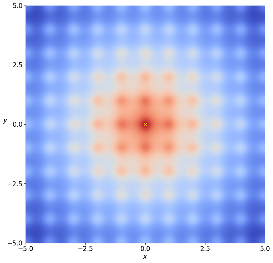
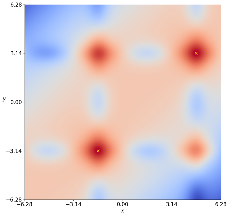
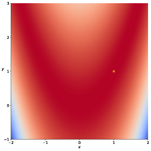
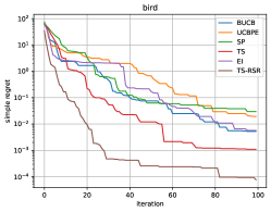
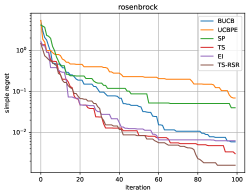
We tested our algorithm against a range of batch BO algorithms on three nonconvex functions, with a batch size of $m=5$: Ackley function, Bird function, and Rosenbrock (all in two dimensions); we note that we picked these test functions before running the experiments, and thus no “cherry picking” of test functions was done. The heatmaps of the three functions are depicted in Figure 1. The performance of our algorithm is compared against the following competitors: namely Batch UCB (BUCB, [Desautels et al., 2014]), Thompson Sampling (TS, [Kandasamy et al., 2018]), GP-UCB with pure exploitation (UCBPE, [Contal et al., 2013]), Fully Distributed Bayesian Optimization with Stochastic Policies (SP, [Garcia-Barcos and Martinez-Cantin, 2019a]), as well as a sequential kriging version of Expected Improvement (EI, [Zhan and Xing, 2020], [Hunt, 2020]). Our experimental setup is as follows. For the GP prior, we use the Matern kernel with $\nu$ parameter set as $\nu=1.5$. For the likelihood noise, we set $\epsilon\sim N(0,\sigma_{n}^{2})$, where $\sigma_{n}=0.001$. We compute the performance of the algorithms across 10 runs, where for each run, each algorithm has access to the same random initialization dataset with 15 samples. Finally, we note that in a practical implementation of our algorithm, for any given $t$ and $i\in[m]$, it may happen that $\tilde{f}_{t,i}^{*}<\mu_{t}(x)$, in which case the algorithm will simply pick out the action $x$ with the highest $\mu_{t}(x)$. While such a situation does not affect the theoretical convergence, for better empirical performance that encourages more diversity, we resample $\tilde{f}_{t,i}^{*}$ whenever $\tilde{f}_{t,i}^{*}<\max_{x}\mu_{t}(x)$, until $\tilde{f}_{t,i}^{*}>\max_{x}\mu_{t}(x)$.

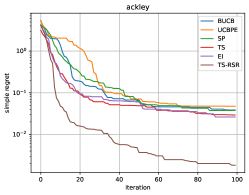
As we see in Figure 2, our algorithm strongly outperforms the other algorithms for both the Ackley and Bird functions, whilst also outperforming other algorithms on Rosenbrock. To get a better sense of the strength of the algorithm over its competitors, we consider Table 1. In this table, we normalize the simple regret attained by an algorithm for a test function at the final iteration $(150)$ by the simple regret attained by the best performing algorithm for that test function. In other words, the best performing algorithm for a test function will attain a ratio of 1 (which is good), and a badly performing algorithm might have a ratio significantly higher than 1. As we can see, $\mathrm{TS-RSR}$ attains the lowest ratio ($1.0$) across all three test functions, indicating its strength over the other algorithms. Moreover, in the last column of the table, where we show the average performance ratio of each algorithm across the three test functions, we see that $\mathrm{TS-RSR}$ is an order of magnitude better than the closest competitor (TS).

Refer to caption
Refer to caption
Refer to caption
Figure 1: Test functions on the numerical experiments (Ackley on the left, Bird in the middle, Rosenbrock on the right)
Refer to caption
Refer to caption
Refer to caption
Figure 2: Simple regret, batch size $m=5$. Each curve is the average of 10 runs.
Table 1: Ratio of simple regret at the 100-th iteration to that of the best algorithm for the test function, batch size $m=5$ (the lower the ratio, the better)

Algorithm Ackley Bird Rosenbrock Average Ratio
BUCB 21.2 67.9 3.7 30.9
UCBPE 26.0 251.4 43.6 107.0
SP 20.6 384.8 25.2 143.5
TS 16.1 14.1 1.9 10.7
EI 14.4 74.1 4.0 30.8
TS-RSR $\mathbf{1.0}$ $\mathbf{1.0}$ $\mathbf{1.0}$ $\mathbf{1.0}$

7 Conclusion

In this paper, we introduced a new algorithm, $\mathrm{TS-RSR}$, for the problem of batch BO. We provide strong theoretical guarantees for our algorithm via a novel analysis, which may be of independent interest to researchers interested in frequentist IDS methods for BO. Moreover, we confirm the efficacy of our algorithm on a range of simulation problems, where we attain strong, state-of-the-art performance. We believe that our algorithm can serve as a new benchmark in batch BO, and as a buiding block for more effective batch BO in practical applications.

8 Acknowledgement

This work is supported by NSF AI institute: 2112085, NSF ECCS: 2328241, NIH R01LM014465, and NSF CPS: 2038603.

References

  • [Adachi et al., 2023] Adachi, M., Hayakawa, S., Hamid, S., Jørgensen, M., Oberhauser, H., and Osborne, M. A. (2023). SOBER: Highly Parallel Bayesian Optimization and Bayesian Quadrature over Discrete and Mixed Spaces. arXiv:2301.11832 [cs, math, stat].
  • [Azimi et al., 2010] Azimi, J., Fern, A., and Fern, X. Z. (2010). Batch Bayesian Optimization via Simulation Matching.
  • [Baek and Farias, 2023] Baek, J. and Farias, V. (2023). Ts-ucb: Improving on thompson sampling with little to no additional computation. In International Conference on Artificial Intelligence and Statistics, pages 11132–11148. PMLR.
  • [Chen et al., 2022] Chen, Y., Dong, P., Bai, Q., Dimakopoulou, M., Xu, W., and Zhou, Z. (2022). Society of agents: Regret bounds of concurrent thompson sampling. Advances in Neural Information Processing Systems, 35:7587–7598.
  • [Contal et al., 2013] Contal, E., Buffoni, D., Robicquet, A., and Vayatis, N. (2013). Parallel gaussian process optimization with upper confidence bound and pure exploration. In Joint European Conference on Machine Learning and Knowledge Discovery in Databases, pages 225–240. Springer.
  • [Dai et al., 2020] Dai, Z., Low, B. K. H., and Jaillet, P. (2020). Federated bayesian optimization via thompson sampling. Advances in Neural Information Processing Systems, 33:9687–9699.
  • [Daxberger and Low, 2017] Daxberger, E. A. and Low, B. K. H. (2017). Distributed batch gaussian process optimization. In International conference on machine learning, pages 951–960. PMLR.
  • [De Palma et al., 2019] De Palma, A., Mendler-Dünner, C., Parnell, T., Anghel, A., and Pozidis, H. (2019). Sampling Acquisition Functions for Batch Bayesian Optimization. arXiv:1903.09434 [cs, stat].
  • [Desautels et al., 2014] Desautels, T., Krause, A., and Burdick, J. W. (2014). Parallelizing exploration-exploitation tradeoffs in gaussian process bandit optimization. Journal of Machine Learning Research, 15:3873–3923.
  • [Frazier, 2018] Frazier, P. I. (2018). A tutorial on bayesian optimization. arXiv preprint arXiv:1807.02811.
  • [Garcia-Barcos and Martinez-Cantin, 2019a] Garcia-Barcos, J. and Martinez-Cantin, R. (2019a). Fully distributed bayesian optimization with stochastic policies. arXiv preprint arXiv:1902.09992.
  • [Garcia-Barcos and Martinez-Cantin, 2019b] Garcia-Barcos, J. and Martinez-Cantin, R. (2019b). Fully Distributed Bayesian Optimization with Stochastic Policies. arXiv:1902.09992 [cs, stat].
  • [Garrido-Merchán and Hernández-Lobato, 2019] Garrido-Merchán, E. C. and Hernández-Lobato, D. (2019). Predictive entropy search for multi-objective bayesian optimization with constraints. Neurocomputing, 361:50–68.
  • [Gong et al., 2019] Gong, C., Peng, J., and Liu, Q. (2019). Quantile stein variational gradient descent for batch bayesian optimization. In International Conference on machine learning, pages 2347–2356. PMLR.
  • [Gonzalez et al., 2015] Gonzalez, J., Dai, Z., Hennig, P., and Lawrence, N. (2015). Batch Bayesian Optimization via Local Penalization.
  • [Hennig and Schuler, 2012] Hennig, P. and Schuler, C. J. (2012). Entropy search for information-efficient global optimization. Journal of Machine Learning Research, 13(6).
  • [Hernández-Lobato et al., 2015] Hernández-Lobato, J. M., Gelbart, M., Hoffman, M., Adams, R., and Ghahramani, Z. (2015). Predictive entropy search for bayesian optimization with unknown constraints. In International conference on machine learning, pages 1699–1707. PMLR.
  • [Hernández-Lobato et al., 2017] Hernández-Lobato, J. M., Requeima, J., Pyzer-Knapp, E. O., and Aspuru-Guzik, A. (2017). Parallel and distributed thompson sampling for large-scale accelerated exploration of chemical space. In International conference on machine learning, pages 1470–1479. PMLR.
  • [Hunt, 2020] Hunt, N. (2020). Batch Bayesian optimization. PhD thesis, Massachusetts Institute of Technology.
  • [Hvarfner et al., 2022] Hvarfner, C., Hutter, F., and Nardi, L. (2022). Joint entropy search for maximally-informed bayesian optimization. Advances in Neural Information Processing Systems, 35:11494–11506.
  • [Kandasamy et al., 2018] Kandasamy, K., Krishnamurthy, A., Schneider, J., and Póczos, B. (2018). Parallelised bayesian optimisation via thompson sampling. In International Conference on Artificial Intelligence and Statistics, pages 133–142. PMLR.
  • [Kaufmann et al., 2012] Kaufmann, E., Cappé, O., and Garivier, A. (2012). On bayesian upper confidence bounds for bandit problems. In Artificial intelligence and statistics, pages 592–600. PMLR.
  • [Kirschner and Krause, 2018] Kirschner, J. and Krause, A. (2018). Information directed sampling and bandits with heteroscedastic noise. In Conference On Learning Theory, pages 358–384. PMLR.
  • [Ma et al., 2023] Ma, H., Zhang, T., Wu, Y., Calmon, F. P., and Li, N. (2023). Gaussian max-value entropy search for multi-agent bayesian optimization. arXiv preprint arXiv:2303.05694.
  • [Nava et al., 2022] Nava, E., Mutný, M., and Krause, A. (2022). Diversified Sampling for Batched Bayesian Optimization with Determinantal Point Processes. arXiv:2110.11665 [cs, stat].
  • [Russo and Van Roy, 2014] Russo, D. and Van Roy, B. (2014). Learning to optimize via information-directed sampling. Advances in Neural Information Processing Systems, 27.
  • [Shah and Ghahramani, 2015] Shah, A. and Ghahramani, Z. (2015). Parallel predictive entropy search for batch global optimization of expensive objective functions. Advances in neural information processing systems, 28.
  • [Srinivas et al., 2009] Srinivas, N., Krause, A., Kakade, S. M., and Seeger, M. (2009). Gaussian process optimization in the bandit setting: No regret and experimental design. arXiv preprint arXiv:0912.3995.
  • [Takeno et al., 2020] Takeno, S., Fukuoka, H., Tsukada, Y., Koyama, T., Shiga, M., Takeuchi, I., and Karasuyama, M. (2020). Multi-fidelity bayesian optimization with max-value entropy search and its parallelization. In International Conference on Machine Learning, pages 9334–9345. PMLR.
  • [Vakili et al., 2021] Vakili, S., Khezeli, K., and Picheny, V. (2021). On information gain and regret bounds in gaussian process bandits. In International Conference on Artificial Intelligence and Statistics, pages 82–90. PMLR.
  • [Vershynin, 2018] Vershynin, R. (2018). High-dimensional probability: An introduction with applications in data science, volume 47. Cambridge university press.
  • [Wang and Jegelka, 2017] Wang, Z. and Jegelka, S. (2017). Max-value entropy search for efficient bayesian optimization. In International Conference on Machine Learning, pages 3627–3635. PMLR.
  • [Wang et al., 2016] Wang, Z., Zhou, B., and Jegelka, S. (2016). Optimization as estimation with gaussian processes in bandit settings. In Artificial Intelligence and Statistics, pages 1022–1031. PMLR.
  • [Zhan and Xing, 2020] Zhan, D. and Xing, H. (2020). Expected improvement for expensive optimization: a review. Journal of Global Optimization, 78(3):507–544.

Appendix

8.1 Facts from information theory

We have the following result (Lemma 5.3 in [Srinivas et al., 2009]), which states that the information gain for any set of selected points can be expressed in terms of predictive variances.

Lemma 4.

For any positive integer $t$, denoting $\bm{f}_{t}$ as $\{f(x_{i})\}_{i=1}^{t}$, we have

$\displaystyle I(\bm{y}_{t};\bm{f}_{t})=\frac{1}{2}\sum_{i=1}^{t}\log\left(1+\sigma_{n}^{-2}\sigma_{t-1}^{2}(x_{t})\right)$

8.2 Concentration results for $Sum_{1}$ and $Sum_{2}$

In this section, we seek to bound $Sum_{1}$ and $Sum_{2}$ using martingale concentration inequalities. We first provide a (standard) martingale concentration inequality for subGaussian martingales.

Lemma 5 (Azuma-Hoeffding [Vershynin, 2018]).

Let $\mathcal{F}_{i}$ be a sequence of filtrations, and suppose $X_{i+1}$ is a sequence of random variables that is adapted to $\mathcal{F}_{i}$, such that $\mathbb{E}[X_{i+1}\mid\mathcal{F}_{i}]=0$, and $X_{i+1}\mid\mathcal{F}_{i}$ is $c_{i}^{2}$-subGaussian, i.e.

$$\mathbb{E}\left[\exp(\lambda X_{i+1})\mid\mathcal{F}_{i}\right]\leqslant\exp(\lambda^{2}c_{i}^{2}/2)\forall\lambda>0.$$

Suppose $c_{i}\leqslant c$ for all $i$. Then,

$\displaystyle P\left(\sum_{i=1}^{n}X_{i}\geqslant t\right)\leqslant\exp\left(-\frac{t^{2}}{2nc^{2}}\right).$

In particular, with probability at least $1-\delta$,

$\displaystyle\sum_{i=1}^{n}X_{i}\leqslant c\sqrt{2n\log(1/\delta)}.$

We next provide a martingale concentration inequality result for the term $Sum_{1}$, which takes the form $Sum_{1}=\sum_{t=0}^{T-1}\sum_{i=1}^{m}f^{*}-\tilde{f}_{t,i}^{*}$.

Lemma 6 (Bound for $Sum_{1}$).

Let $\tilde{f}_{t,i}^{*}$ denote an iid sample from $f^{*}\>|\>\mathcal{F}_{t}$. Then, for any $\delta>0$, with probability at least $1-\delta$, we have

$\displaystyle\sum_{t=0}^{T-1}\sum_{i=1}^{m}f^{*}-\tilde{f}_{t,i}^{*}\leqslant 2\sqrt{Tm\log(1/\delta)}.$
Proof.

Let $x^{*}$ be the maximizer of the sampled $f$, i.e. $f(x^{*})=f^{*}$. Then, we observe that we have the following:

$\displaystyle\ \sum_{t=0}^{T-1}\sum_{i=1}^{m}f^{*}-\tilde{f}_{t,i}^{*}$
$\displaystyle=$ $\displaystyle\ \sum_{t=0}^{T-1}\sum_{i=1}^{m}f(x^{*})-\tilde{f}_{t,i}(x^{*})+\tilde{f}_{t,i}(x^{*})-\tilde{f}_{t,i}^{*}$
$\displaystyle\leqslant$ $\displaystyle\ \sum_{t=0}^{T-1}\sum_{i=1}^{m}f(x^{*})-\tilde{f}_{t,i}(x^{*}),$

where we note that the inequality follows since $\tilde{f}_{t,i}(x^{*})$ denotes the random draw of $x^{*}$ at the same time when $\tilde{f}_{t,i}^{*}$ was sampled, such that $\tilde{f}_{t,i}(x^{*})\leqslant\tilde{f}_{t,i}^{*}$ has to hold. The result then follows by observing that $f(x^{*})-\tilde{f}_{t,i}(x^{*})$ is a centered, $2\sigma_{t}^{2}(x^{*})$ subGaussian martingale, the fact that $\sigma_{t}^{2}(x^{*})\leqslant 1$, and applying Lemma 5 to the sum

$\displaystyle\sum_{t=0}^{T-1}\sum_{i=1}^{m}f(x^{*})-\tilde{f}_{t,i}(x^{*}).$

We next bound $Sum_{2}$.

Lemma 7.

Let $\tilde{f}_{t,i}$ denotes a random sample from $f(x_{t+1,i}^{\mathrm{TS-RSR}})\mid\mathcal{F}_{t}$. Then, with probability at least $1-2\delta$, we have

=\displaystyle= t=0T1i=1m(μt(xt+1,iTSRSR)f(xt+1,iTSRSR))superscriptsubscript𝑡0𝑇1superscriptsubscript𝑖1𝑚subscript𝜇𝑡superscriptsubscript𝑥𝑡1𝑖TSRSR𝑓superscriptsubscript𝑥𝑡1𝑖TSRSR\displaystyle\ \sum_{t=0}^{T-1}\sum_{i=1}^{m}(\mu_{t}(x_{t+1,i}^{\mathrm{TS-RSR}})-f(x_{t+1,i}^{\mathrm{TS-RSR}}))
=\displaystyle= t=0T1i=1m(μt(xt+1,iTSRSR)f~t,i(xt+1,iTSRSR))Sum2,1subscriptsuperscriptsubscript𝑡0𝑇1superscriptsubscript𝑖1𝑚subscript𝜇𝑡superscriptsubscript𝑥𝑡1𝑖TSRSRsubscript~𝑓𝑡𝑖superscriptsubscript𝑥𝑡1𝑖TSRSR𝑆𝑢subscript𝑚21\displaystyle\ \underbrace{\sum_{t=0}^{T-1}\sum_{i=1}^{m}(\mu_{t}(x_{t+1,i}^{\mathrm{TS-RSR}})-\tilde{f}_{t,i}(x_{t+1,i}^{\mathrm{TS-RSR}}))}_{Sum_{2,1}}
$\displaystyle+\underbrace{\sum_{t=0}^{T-1}\sum_{i=1}^{m}(\tilde{f}_{t,i}(x_{t+1,i}^{\mathrm{TS-RSR}})-f(x_{t+1,i}^{\mathrm{TS-RSR}}))}_{Sum_{2,2}}$
$\displaystyle\leqslant$ $\displaystyle\ 4\sqrt{Tm\log(1/\delta)}$
Proof.

The result follows from applying Lemma 5 to each of $Sum_{2,1}$ and $Sum_{2,2}$. ∎