Quantum Advantage in Reversing Unknown Unitary Evolutions

Yu-Ao Chen Yu-Ao Chen and Yin Mo contributed equally to this work. Thrust of Artificial Intelligence, Information Hub,The Hong Kong University of Science and Technology (Guangzhou), Guangdong 511453, China Yin Mo11footnotemark: 1 Thrust of Artificial Intelligence, Information Hub,The Hong Kong University of Science and Technology (Guangzhou), Guangdong 511453, China Yingjian Liu Thrust of Artificial Intelligence, Information Hub,The Hong Kong University of Science and Technology (Guangzhou), Guangdong 511453, China Lei Zhang Thrust of Artificial Intelligence, Information Hub,The Hong Kong University of Science and Technology (Guangzhou), Guangdong 511453, China Xin Wang felixxinwang@hkust-gz.edu.cn Thrust of Artificial Intelligence, Information Hub,The Hong Kong University of Science and Technology (Guangzhou), Guangdong 511453, China
Abstract

We introduce the Quantum Unitary Reversal Algorithm (QURA), a deterministic and exact approach to universally reverse arbitrary unknown unitary transformations using $\mathcal{O}(d^{2})$ calls of the unitary, where $d$ is the system dimension. Our construction resolves a fundamental problem of time-reversal simulations for closed quantum systems by affirming the feasibility of reversing any unitary evolution without knowing the exact process. The algorithm also provides the construction of a key oracle for unitary inversion in quantum algorithm frameworks such as quantum singular value transformation. Notably, our work demonstrates that compared with classical methods relying on process tomography, reversing an unknown unitary on a quantum computer holds a quadratic quantum advantage in computation complexity. QURA ensures an exact unitary inversion while the classical counterpart can never achieve exact inversion using a finite number of unitary calls.

1 Introduction

Quantum mechanics offers an intricate and robust framework that is essential for delving into the microscopic realm, as well as for the innovation of groundbreaking technologies in quantum computingΒ [1, 2, 3, 4, 5], quantum communicationΒ [6, 7, 8], and quantum sensingΒ [9]. At the heart of this framework are quantum unitaries, which encapsulates the dynamics of closed quantum systems, governing their evolution over time in accordance with the Schrodinger equationΒ [10].

Reversibility is a cornerstone of quantum unitary operations, reflecting the fundamental behavior of closed quantum systems. These systems evolve through time according to unitary operators $U=e^{-iHt}$ with a Hamiltonian $H$ and time $t$, which are inherently reversible via the inverse operation $U^{-1}=e^{iHt}$, distinguishing quantum computing from its classical counterpart with irreversible operations. This reversibility of quantum unitary operation not only differentiates quantum computation from classical computation, but also aligns with the time-reversal symmetry intrinsic to quantum mechanics. The time-reversal simulation of an unknown unitary transformation aims to simulate the backward evolution of a quantum state, analogous to running the arrow of time in reverse. Such a task is not only theoretically compellingΒ [11] but also stands as a testament to our quest for mastering quantum systems and measuring the out-of-time-order correlatorsΒ [12, 13, 14].

The capability to reverse an unknown unitary operation plays a pivotal role within quantum computing, particularly as a ground component in many quantum algorithms. Among these, the Quantum Singular Value Transformation (QSVT)Β [15] emerges as a particularly prominent and comprehensive framework, offering a generalization for a wide array of quantum algorithmsΒ [16]. The implementation of QSVT necessitates the implementation of a block-encoding oracle as well as its unitary inverse so that an invariant subspace can be constructed for polynomial manipulation of the encoded data. While it is easy to reverse a unitary with known established quantum circuits, how to reverse an unknown unitary remains a long-standing open problem. This gap imposes a nontrivial limitation on the capability and practicality of QSVT and other extensionsΒ [17, 18].

The difficulty in reversing an unknown unitary transformation stems from the fact that complete information about a general physical system in nature is often unavailable. To classically simulate the inverse operation $U^{-1}=e^{iHt}$ exactly, it is necessary to fully characterize the unitary or the Hamiltonian. However, obtaining such precise knowledge is often impractical or impossible, especially for complex quantum systems. Process tomographyΒ [19, 20, 21, 22], a technique used to characterize quantum processes, is prohibitively resource-intensive, requiring an impractical number of measurements to exactly characterize a quantum process. This limitation makes the exact reversal of a general unknown unitary extremely challenging with the routine approach of learning and inverting the unitary.

To circumvent the formidable challenge of deducing an unknown unitary, we can draw upon Feynman’s visionary concept of using one quantum system to simulate anotherΒ [23]. This celebrated idea suggests the feasibility of exactly simulating the time-reversal evolution of a closed quantum system by leveraging the original forward evolution process itself and shedding light on demonstrating quantum advantages via quantum simulation. Ref.Β [24] provides positive evidence in this direction by showing a universal probabilistic heralded quantum circuit that implements the exact inverse of an unknown unitary. Ref.Β [25] took a further step by proposing a deterministic and exact protocol to reverse any unknown qubit unitary transformation. Despite these advances, the question of whether an unknown unitary evolution, in general (especially beyond the simple qubit cases to higher dimensions), can be exactly and deterministically reversed in time remains a formidable open challenge in quantum information science.

In this article, we introduce the first universal protocol to reverse any unknown unitary transformation of arbitrary dimension deterministically and exactly with finite calls of the unitary. To prove it, we propose the Quantum Unitary Reversal Algorithm (QURA) to realize the inversion of an arbitrary input $U\in\mathfrak{su}(d)$ by $\mathcal{O}(d^{2})$ calls of $U$, which is potentially near-optimal based on the recent observations and numerical calculations for small-scale $d$ in [25]. The main idea of QURA involves encoding and transforming the information of the gate $U$ into a dedicated subspace corresponding to its inversion $U^{-1}$ within the prepared quantum state. Subsequently, leveraging a duality-based amplitude amplifier, QURA effectively amplifies the specific portion to amplitude $1$, to achieve the time reversal of $U$ exactly and deterministically. Beyond resolving the fundamental question of reversibility of unknown unitary operations, our research illustrates that, in contrast to classical methods that employ process tomography, our approach exhibits a quadratic advantage in computational complexity, and removes the dependency of process error in query complexity, thereby underscoring its advantage in scalability and efficiency.

Refer to caption
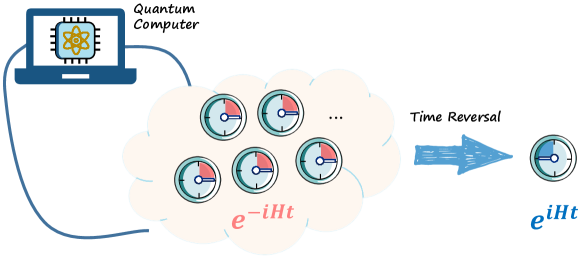
Fig 1: Reversing an unknown unitary with finite calls of the unitary evolution.

2 Quantum Unitary Reversal Algorithm

Refer to caption
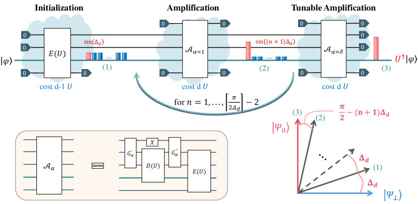
Fig 2: Sketch of Quantum Unitary Reversal Algorithm. This algorithm, akin to the idea of amplitude amplification, is structured in three stages. The input quantum state $|\varphi\rangle$ is initialized into the superposition of the target U†​|Ο†βŸ©superscriptπ‘ˆβ€ ketπœ‘U^{{\dagger}}|\varphi\rangle and the other unwanted components with averaged amplitudes. A β€œDuality-based amplitude amplifier” ${\cal A}_{\alpha=1}$, for which we provide a specific circuit construction shown in the box at the lower left, is then used iteratively to enhance the amplitude of the target state in $\sin{\theta}$ by rotating its angle with a constant angle $\Delta_{d}$. The iteration ends when the angle approaches its maximum before surpassing $\frac{\pi}{2}$. Consequently, the tunable amplifier, denoted as ${\cal A}_{\alpha=\delta}$, completes the angular amplification up to $\frac{\pi}{2}$, giving rise to the inverse of unitary with all ancillary qudits returning to $|0\rangle_{d}$.

According to the unitarity of $U$, the reverse of $U\in\mathfrak{su}(d)$ is also its transpose conjugate as Uβˆ’1=U†superscriptπ‘ˆ1superscriptπ‘ˆβ€ U^{-1}=U^{{\dagger}}. In the following, we illustrate that the transpose conjugate operation of $U$ can be achieved through a general quantum circuit, hence formulating the following theorem:

Theorem 1
For any dimension $d$, there exists a quantum algorithm that exactly and deterministically implements U†superscriptπ‘ˆβ€ U^{\dagger} for arbitrary $d$-dimensional unitary operator $U$, by using at most $d\lceil\frac{\pi}{2\Delta_{d}}\rceil-1$ calls of $U$, where $\Delta_{d}=\arcsin{\frac{1}{d}}$.

RemarkΒ 1 For this theorem, in addition to providing the number of queries to $U$ required by the algorithm to implement U†superscriptπ‘ˆβ€ U^{\dagger}, we also analyze the other required resources. The time cost for this algorithm is ${\cal O}(d)$, and the dimension of the required ancillary qubits is ${\cal O}(d\log(d))$. Detailed discussions and comparisons with classical methods and previous probabilistic protocols will be given in SectionΒ 3.

Proof. We prove Theorem 1 by proposing the Quantum Unitary Reversal Algorithm (QURA) in Algorithm 1 to exactly reverse an unknown $U\in\mathfrak{su}(d)$ with $d\lceil\frac{\pi}{2\Delta_{d}}\rceil-1$ calls of $U$. An intuitive streamline of the algorithm is depicted in FigureΒ 2, where the key element is shown by the vertical red bar, corresponding to the amplitude of the target quantum state in the circuit, which we denote as $|\Psi_{0}\rangle$:

|Ξ¨0⟩=|0⟩dβŠ—|0⟩dβŠ—U†​|Ο†βŸ©dβŠ—|0⟩dβŠ—dβˆ’2,ketsubscriptΞ¨0tensor-producttensor-productsubscriptket0𝑑subscriptket0𝑑superscriptπ‘ˆβ€ subscriptketπœ‘π‘‘superscriptsubscriptket0𝑑tensor-productabsent𝑑2|\Psi_{0}\rangle=|0\rangle_{d}\otimes|0\rangle_{d}\otimes U^{\dagger}|\varphi\rangle_{d}\otimes|0\rangle_{d}^{\otimes d-2}\,, (1)

where $|\cdot\rangle_{d}$ denotes a $d$-dimensional qudit. The amplitude of state $|\Psi_{0}\rangle$ will gradually tend to 1 as the algorithm progresses, at which point U†superscriptπ‘ˆβ€ U^{{\dagger}} is deterministically realized by tracing out the ancillary qudits. Here, we briefly introduce the main idea of this algorithm, with detailed calculations provided in AppendixΒ A.

The algorithm is structured in three stages, wherein the initialization, a subcircuit which we name as β€œintrinsic encoder” $E(U)$ is used to prepare the target state $|\Psi_{0}\rangle$ with some unwanted orthogonal component $|\Psi_{\perp}\rangle$, respective to the vector (1) in FigureΒ 2:

$$E(U)\cdot\left(|0\rangle_{d}\otimes|0\rangle_{d}\otimes|\varphi\rangle_{d}\otimes|0\rangle_{d}^{\otimes d-2}\right)=\sin{\Delta_{d}}|\Psi_{0}\rangle+\cos{\Delta_{d}}|\Psi_{\perp}\rangle\,.$$ (2)

Then the most important module, which we name as β€œDuality-based amplitude amplifier” ${\cal A}_{\alpha}$, is well-designed to adjust the amplitude of $|\Psi_{0}\rangle$. For an input state $|\Psi_{\theta}\rangle=\sin{\theta}|\Psi_{0}\rangle+\cos{\theta}|\Psi_{\perp}\rangle$, ${\cal A}_{\alpha}$ will rotate the angle $\theta$ of the state to

$$\theta\xrightarrow{{\cal A}_{\alpha}}\arcsin(\alpha\sin{\theta})+\Delta_{d},$$ (3)

where by selecting an appropriate $\alpha\in\left[0,1\right]$, arbitrary amplified angle from $\Delta_{d}$ to $\theta+\Delta_{d}$ could be generated. It is noticed that for the special case when $\alpha=1$, ${\cal A}_{\alpha}$ turns to rotate the angle $\theta$ with a constant $\Delta_{d}$.

Different from the conventional amplitude amplification with oraclesΒ [26], the construction of ${\cal A}_{\alpha}$ is based on the β€œintrinsic encoder” $E(U)$ and a β€œshifted decoder” $D(U)$, which are two subcircuits with using $d-1$ and 1 copies of $U$ respectively, satisfying the duality relations:

$\displaystyle D(U)\cdot E(U)\cdot\left(|0\rangle_{d}|0\rangle_{d}\otimes\mathbbm{1}\right)=|+\rangle_{d}|+\rangle_{d}\otimes\mathbbm{1},$ (4)
$\displaystyle E(U)\cdot D(U)\cdot\left(|+\rangle_{d}|+\rangle_{d}\otimes\mathbbm{1}\right)=|0\rangle_{d}|0\rangle_{d}\otimes\mathbbm{1},$ (5)

where $|+\rangle_{d}\coloneqq\frac{1}{\sqrt{d}}\sum_{j=0}^{d-1}|j\rangle_{d}$. It is proved in LemmaΒ S6 from AppendixΒ A that with the help of fixed subcircuits $G^{{}^{\prime}}_{\alpha},G^{{}^{\prime\prime}}_{\alpha}$, and single-qubit gate $X$ in FigureΒ 2, the duality relations enable the module ${\cal A}_{\alpha}$ to amplify the component of $|\Psi_{0}\rangle$ in the way shown in Eq.Β (3).

When the amplitude of $|\Psi_{0}\rangle$ is amplified to 1, U†superscriptπ‘ˆβ€ U^{{\dagger}} is realized deterministically by tracing out the ancillary systems of $|\Psi_{0}\rangle$. To achieve it, the amplifier ${\cal A}_{\alpha=1}$ is executed for $n=\lceil\frac{\pi}{{2\Delta_{d}}}\rceil-2$ times after the initialization. Subsequently, an additional tunable amplifier ${\cal A}_{\alpha=\delta}$ with $\delta=\frac{\cos{\Delta_{d}}}{\sin{((n+1)\Delta_{d}})}$ is required to compensate the residue into $\frac{\pi}{2}$. Especially for the case when $(n+2)\Delta_{d}=\frac{\pi}{2}$, the tunable amplifier ${\cal A}_{\alpha=\delta}$ is exactly ${\cal A}_{\alpha=1}$. It is also worth noticing that since ${\cal A}_{\alpha=1}$ works as a constant amplifier, independent of the former angle $\theta$, the tunable amplifier is flexible to move into any section after the initialization.

The querying complexity of Algorithm 1, namely, the number of calls of $U$ is calculated by counting the overhead of $E(U)$ and $D(U)$. According to the algorithm, ${\cal A}_{\alpha}$ is executed for $n+1$ times, with respect to the consumption of $d(n+1)$ copies of $U$. While the initialization takes $d-1$ calls of $U$. The total number of calls of $U$ is then $d\lceil\frac{\pi}{{2\Delta_{d}}}\rceil-1$, which is at most $\frac{\pi}{2}d^{2}$ for large $d$. β– β– \blacksquare.

Here we point out that the specific circuit realization of the two most critical subcircuits, $E(U)$ and $D(U)$, is inspired by the observation that the complex conjugate of an arbitrary unitary matrix $U\in\mathfrak{su}(d)$ can be achieved with using $d-1$ instances of this gate in parallelΒ [27]. Then the unitary inverse can be realized through the following relationship

U†=(Uβˆ—)T=1dβ€‹βˆ‘j,k=0dβˆ’1Zj​Xk​Uβˆ—β€‹Zβˆ’j​Xk,superscriptπ‘ˆβ€ superscriptsuperscriptπ‘ˆπ‘‡1𝑑superscriptsubscriptπ‘—π‘˜0𝑑1superscript𝑍𝑗superscriptπ‘‹π‘˜superscriptπ‘ˆsuperscript𝑍𝑗superscriptπ‘‹π‘˜U^{\dagger}=(U^{*})^{T}=\dfrac{1}{d}\sum_{j,k=0}^{d-1}Z^{j}X^{k}U^{*}Z^{-j}X^{k}\,, (6)

which follows from the unitary transpose representation $U^{T}=\dfrac{1}{d}\sum_{j,k=0}^{d-1}Z^{j}X^{k}UZ^{-j}X^{k}$ where $Z=\sum^{d-1}_{j=0}\omega^{j}|j\rangle\!\langle j|$ with $\omega=e^{2\pi i/d}$, and $X=\sum^{d-1}_{j=0}|(j+1)\operatorname{mod}d\rangle\!\langle j|$ are the clock and shift operators, respectively. Hence, the key point is to design quantum circuits that could realize the transpose of an unknown unitary, which is resolved in our algorithm. For the multi-qubit version, we provide an alternative version of the modified encoder and decoder based on the tensor product decomposition, which may yield a slightly more friendly circuit, with details in Appendix C.

Now we give the detailed procedure for QURA in AlgorithmΒ 1, where the notation used in this algorithm is the same as in the discussion of Theorem 1. $m$ corresponds to the number of queries for the gate $U$. $|\Psi_{0}\rangle$ corresponds to the target state U†​|Ο†βŸ©superscriptπ‘ˆβ€ ketπœ‘U^{\dagger}|\varphi\rangle is provided by Eq.Β (1). $E(U)$ is the intrinsic encoder that satisfies Eq.Β (2), and $|\Psi_{\perp}\rangle$ represents the unwanted component orthogonal to $|\Psi_{0}\rangle$ obtained after applying $E(U)$. The specific circuit implementations for each module can be found in the AppendixΒ A, and the whole circuit for inverting qubit-unitary $U$ with querying it five times based on this algorithm has been specifically presented in a recent workΒ [28]. We also note that QURA can also be understood as a hybrid digital-analog quantum algorithm that simulates the unitary inverse via plugging the original unitary evolution into quantum circuits with open slots.

0:Β Β input state $|\varphi\rangle$, $m$ copies of evolution $U$ in a $d$-dimensional system.
0:Β Β output state U†​|Ο†βŸ©superscriptπ‘ˆβ€ ketπœ‘U^{\dagger}|\varphi\rangle after the time-reversed evolution U†superscriptπ‘ˆβ€ U^{{\dagger}}.
1:Β Β Prepare the input state $|\psi\rangle\leftarrow|0\rangle\otimes|0\rangle_{d}\otimes|0\rangle_{d}\otimes|\varphi\rangle_{d}\otimes|0\rangle_{d}^{\otimes d-2}$.
2:Β Β Apply $E(U)$ to $|\psi\rangle$ gives $|\psi\rangle\leftarrow\left(I_{2}\otimes E(U)\right)|\psi\rangle=\sin{\Delta_{d}}|\Psi_{0}\rangle+\cos{\Delta_{d}}|\Psi_{\perp}\rangle$.
3:Β Β forΒ n←1,2,3,…,βŒˆΟ€2​ΔdβŒ‰βˆ’2←𝑛123β€¦πœ‹2subscriptΔ𝑑2n\leftarrow 1,2,3,\ldots,\lceil\dfrac{\pi}{{2\Delta_{d}}}\rceil-2Β do
4:Β Β Β Β Β Apply ${\cal A}_{\alpha=1}$ to $|\psi\rangle$ gives $|\psi\rangle\leftarrow{\cal A}_{\alpha=1}|\psi\rangle=\sin{((n+1)\Delta_{d})}|\Psi_{0}\rangle+\cos{((n+1)\Delta_{d})}|\Psi_{\perp}\rangle$.
5:Β Β endΒ for
6:Β Β Set $\delta\leftarrow\cos\left(\Delta_{d}\right)/\sin\left((n+1)\Delta_{d}\right)$ and output ${\cal A}_{\alpha=\delta}|\psi\rangle=|\Psi_{0}\rangle$.
AlgorithmΒ 1 Quantum Unitary Reversal Algorithm (QURA)

3 Quantum Advantage and Comparison

Quantum computers offer a computational paradigm capable of outperforming classical computers on specific tasks by harnessing quantum mechanical principles. The field has seen significant interest due to its potential to disrupt conventional computational domains, such as cryptographyΒ [1], database searchingΒ [2], and quantum simulationΒ [3]. As quantum hardware advances, recent results have shown quantum advantages in specific mathematical problemsΒ [29, 30, 31].

An emerging direction is to explore whether quantum computing can extend such supremacy to more practical and operational domains. Specifically, Ref.Β [32] shows that for certain learning tasks, quantum computers have substantial advantages over classical processing of measurements of quantum states. Unlike this learning paradigm, our focus is on showcasing the quantum advantage inherent in simulating the temporally reversed dynamics of quantum systems. In this section, we compare QURA with the existing quantum and classical methods, in terms of the error of output process, the probability of success, the computational complexity, query complexity of $U$ and the number of ancilla qubits. The results are summarized in TableΒ 1.

Method Error Successful Probability Computational complexity Query Number of ancillas
QURA (this work) 00 $1$ ${\cal O}\left(d\right)$ ${\cal O}\left(d^{2}\right)$ ${\cal O}\left(d\log(d)\right)$ qubits
Ref.Β [33] 00 $1-(1-1/d^{2})^{\lfloor(k+1)/d\rfloor}$ ${\cal O}\left(k/d\right)$ $k$ ${\cal O}\left(d\log(d)\right)$ qubits
Ref.Β [33] (take $k={\cal O}(d^{3})$) 00 ${\cal O}(1)$ ${\cal O}\left(d^{2}\right)$ ${\cal O}\left(d^{3}\right)$ ${\cal O}\left(d\log(d)\right)$ qubits
Tomo $U$ and prepare U†superscriptπ‘ˆβ€ U^{\dagger} $\epsilon$ $1$ ${\cal O}\left(d^{2}/\epsilon\right)$ ${\cal O}\left(d^{2}/\epsilon\right)$ $\Theta(d^{2})$ cbits
Tomo $U$ and $\rho$, and prepare U†​ρ​Usuperscriptπ‘ˆβ€ πœŒπ‘ˆU^{\dagger}\rho U $\epsilon$ $1$ ${\cal O}\left(d^{2}/\epsilon^{2}+d^{2.37}\right)$ ${\cal O}\left(d^{2}/\epsilon^{2}\right)$ $\Theta\left(d^{2}\right)$ cbits
Table 1: The table of quantum and classical protocols to realize unitary inversion. Here the error is measured in trace norm distance, and $d$ is the dimension of the input unitary. The second row corresponds to the probabilistic quantum methodΒ [33], where $k$ is the number of queries of $U$ in it; the required resources for the classical method are based on the studies inΒ [19, 20, 21, 22, 34, 35, 36]

On the one hand, the existing quantum method to reverse an unknown unitary is an iterative teleportation-based protocol, which works probabilisticallyΒ [33]. During each iteration, U†superscriptπ‘ˆβ€ U^{\dagger} can be generated deterministically with a non-zero probability. If it fails, another application of $U$ and the corresponding Pauli gates are performed to recover the state to continue to the next iteration, so that it works quite efficiently as the probability of failure exponentially tends to zero. For large $d$, to better compare with our scheme, we find that to ensure the successful probablility in ${\cal O}\left(1\right)$, the number of queries is at least in ${\cal O}\left(d^{3}\right)$, and the number of iterations will be in ${\cal O}\left(d^{2}\right)$.

On the other hand, the classical approach must obtain its classical information through process tomography, and store it in a classical computer. To tomograph such a unitary with an $\epsilon$-error in the diamond norm, the computational complexity will be in ${\cal O}(d^{2}/\epsilon)$Β [19, 20, 21, 22]. Subsequently, to implement U†superscriptπ‘ˆβ€ U^{\dagger}, we need $\Theta(d^{2})$ algorithm execution time to compute U†superscriptπ‘ˆβ€ U^{\dagger} classically, and ${\cal O}(d^{2})$ time cost to prepare the operation of it. If one wishes to obtain the whole matrix of U​ρ​Uβ€ π‘ˆπœŒsuperscriptπ‘ˆβ€ U\rho U^{\dagger}, we also need to perform the tomography of state $\rho$ with the computational time ${\cal O}(d^{2}/\delta^{2})$ to achieve $\delta$ accuracyΒ [34, 35], followed ${\cal O}(d^{2.37})$ time cost of algorithm to compute state U​ρ​Uβ€ π‘ˆπœŒsuperscriptπ‘ˆβ€ U\rho U^{\dagger} based on the best matrix multiplication algorithm [36].

In contrast, our scheme only requires running the β€œduality-based amplitude amplifier” for ${\cal O}(d)$ times, with $d-1$ instances of $U$ being utilized in parallel in each amplifier. The number of queries to $U$ also reduces to ${\cal O}(d^{2})$. In summary, the previous quantum algorithm is exact but not deterministic, and classical algorithms are deterministic but not exact, whereas QURA is both exact and deterministic. Meanwhile, QURA shows advantages in computational complexity, query complexity, and the number of ancilla qubits when compared to other methods.

4 Concluding remarks

We have introduced the Quantum Unitary Reversal Algorithm (QURA), the first deterministic and exact approach to reverse unknown quantum time evolutions with arbitrary dimensions. By harnessing the inherent dynamics of quantum systems and developing novel duality-based amplitude amplification techniques, we have demonstrated that QURA can universally reverse any unitary transformation with perfect fidelity and success probability, using ${\cal O}(d^{2})$ calls of the unitary and execution time ${\cal O}(d)$. One key technical contribution in QURA is the utilization of techniques to implement amplitude amplification without the need for oracles, which provides valuable insights into the design of quantum algorithms for specific tasks. Our algorithm can be also viewed as a hybrid digital-analog quantum algorithm, combining time-evolutions of quantum systems into quantum circuits with open slots.

While the observation from Ref.Β [25] hinting that $d^{2}-1$ calls of the unitary are necessary for universal unitary inversion for qudit systems with $d>2$, QURA not only showed that unknown unitary operation can be reversed in general but also probably already achieved the near-optimal performance. In particular, our result can be utilized in many quantum algorithms necessitating the oracle implementation of unknown unitary inversion operators. Future research may focus on optimizing the performance of QURA and exploring its applicability in diverse quantum computing and simulation tasks. Additionally, it will be interesting to investigate whether ${\cal O}(d^{2})$ calls are optimal for universal unitary inversion. Such investigations promise to deepen our understanding of unitary transformations and open up new avenues for quantum algorithms by transforming unknown quantum dynamics.

Our work in particular demonstrates that QURA can obtain a quadratic improvement over classical methods relying on quantum tomography. QURA is an exact algorithm and thus can remove the effect of algorithm precision on the query complexity of input unitaries, which is unavoidable in classical methods. We believe these results contribute to the ongoing exploration of quantum advantage and have the potential for developing meaningful and practical quantum applications.

Acknowledgement

Y.-A. C. and Y. M. contributed equally to this work. We would like to thank Zhan Yu, Xuanqiang Zhao, and Keming He for their helpful comments. This work was supported by the Start-up Fund (No. G0101000151) from The Hong Kong University of Science and Technology (Guangzhou), the Guangdong Provincial Quantum Science Strategic Initiative (No. GDZX2303007), and the Education Bureau of Guangzhou Municipality.

References

  • [1] PeterΒ W. Shor. Polynomial-Time Algorithms for Prime Factorization and Discrete Logarithms on a Quantum Computer. SIAM Journal on Computing, 26(5):1484–1509, oct 1997.
  • [2] LovΒ K Grover. A fast quantum mechanical algorithm for database search. In Proceedings of the twenty-eighth annual ACM symposium on Theory of computing - STOC ’96, pages 212–219, New York, New York, USA, 1996. ACM Press.
  • [3] Seth Lloyd. Universal Quantum Simulators. Science, 273(5278):1073–1078, aug 1996.
  • [4] AndrewΒ M Childs and Wim van Dam. Quantum algorithms for algebraic problems. Reviews of Modern Physics, 82(1):1–52, jan 2010.
  • [5] AndrewΒ M Childs, Debbie Leung, Laura Mančinska, and Maris Ozols. A framework for bounding nonlocality of state discrimination. Communications in Mathematical Physics, 323(3):1121–1153, 2013.
  • [6] CharlesΒ H Bennett, Gilles Brassard, Claude CrΓ©peau, Richard Jozsa, Asher Peres, and WilliamΒ K Wootters. Teleporting an unknown quantum state via dual classical and Einstein-Podolsky-Rosen channels. Physical Review Letters, 70(13):1895–1899, mar 1993.
  • [7] Dik Bouwmeester, Jian-Wei Pan, Klaus Mattle, Manfred Eibl, Harald Weinfurter, and Anton Zeilinger. Experimental quantum teleportation. Nature, 390(6660):575–579, 1997.
  • [8] C.H. Bennett, P.W. Shor, J.A. Smolin, and A.V. Thapliyal. Entanglement-assisted capacity of a quantum channel and the reverse Shannon theorem. IEEE Transactions on Information Theory, 48(10):2637–2655, oct 2002.
  • [9] ChristianΒ L Degen, FΒ Reinhard, and Paola Cappellaro. Quantum sensing. Reviews of modern physics, 89(3):35002, 2017.
  • [10] DavidΒ J Griffiths and DarrellΒ F Schroeter. Introduction to quantum mechanics. Cambridge university press, 2018.
  • [11] Yakir Aharonov, Jeeva Anandan, Sandu Popescu, and Lev Vaidman. Superpositions of time evolutions of a quantum system and a quantum time-translation machine. Physical Review Letters, 64(25):2965, 1990.
  • [12] Juan Maldacena, StephenΒ H Shenker, and Douglas Stanford. A bound on chaos. Journal of High Energy Physics, 2016(8):1–17, 2016.
  • [13] Jun Li, Ruihua Fan, Hengyan Wang, Bingtian Ye, Bei Zeng, Hui Zhai, Xinhua Peng, and Jiangfeng Du. Measuring out-of-time-order correlators on a nuclear magnetic resonance quantum simulator. Physical Review X, 7(3):31011, 2017.
  • [14] Martin GΓ€rttner, JustinΒ G Bohnet, Arghavan Safavi-Naini, MichaelΒ L Wall, JohnΒ J Bollinger, and AnaΒ Maria Rey. Measuring out-of-time-order correlations and multiple quantum spectra in a trapped-ion quantum magnet. Nature Physics, 13(8):781–786, 2017.
  • [15] AndrΓ‘s GilyΓ©n, Yuan Su, GuangΒ Hao Low, and Nathan Wiebe. Quantum singular value transformation and beyond: Exponential improvements for quantum matrix arithmetics. In Proceedings of the 51st Annual ACM SIGACT Symposium on Theory of Computing, pages 193–204, Phoenix AZ USA, June 2019. ACM.
  • [16] JohnΒ M. Martyn, ZaneΒ M. Rossi, AndrewΒ K. Tan, and IsaacΒ L. Chuang. Grand Unification of Quantum Algorithms. PRX Quantum, 2(4):040203, dec 2021.
  • [17] Youle Wang, Lei Zhang, Zhan Yu, and Xin Wang. Quantum phase processing and its applications in estimating phase and entropies. Physical Review A, 108(6):062413, dec 2023.
  • [18] Tatsuki Odake, HlΓ©r KristjΓ‘nsson, Philip Taranto, and Mio Murao. Universal algorithm for transforming hamiltonian eigenvalues, December 2023.
  • [19] CharlesΒ H Baldwin, Amir Kalev, and IvanΒ H Deutsch. Quantum process tomography of unitary and near-unitary maps. Physical Review A, 90(1):12110, jul 2014.
  • [20] Gus Gutoski and Nathaniel Johnston. Process tomography for unitary quantum channels. Journal of Mathematical Physics, 55(3):32201, 2014.
  • [21] MΒ Mohseni, AΒ T Rezakhani, and DΒ A Lidar. Quantum-process tomography: Resource analysis of different strategies. Physical Review A, 77(3):032322, mar 2008.
  • [22] Jeongwan Haah, Robin Kothari, Ryan O’Donnell, and Ewin Tang. Query-optimal estimation of unitary channels in diamond distance. In 2023 IEEE 64th Annual Symposium on Foundations of Computer Science (FOCS), pages 363–390. IEEE, 2023.
  • [23] RichardΒ P Feynman. Simulating physics with computers. International Journal of Theoretical Physics, 21(6/7), 1982.
  • [24] MarcoΒ TΓΊlio Quintino, Qingxiuxiong Dong, Atsushi Shimbo, Akihito Soeda, and Mio Murao. Probabilistic exact universal quantum circuits for transforming unitary operations. Physical Review A, 100(6):062339, dec 2019.
  • [25] Satoshi Yoshida, Akihito Soeda, and Mio Murao. Reversing Unknown Qubit-Unitary Operation, Deterministically and Exactly. Physical Review Letters, 131(12), 2023.
  • [26] Gilles Brassard, Peter Hoyer, Michele Mosca, and Alain Tapp. Quantum amplitude amplification and estimation. pages 53–74. 2002.
  • [27] Jisho Miyazaki, Akihito Soeda, and Mio Murao. Complex conjugation supermap of unitary quantum maps and its universal implementation protocol. Physical Review Research, 1(1):013007, aug 2019.
  • [28] Yin Mo, Lei Zhang, Yu-Ao Chen, Yingjian Liu, Tengxiang Lin, and Xin Wang. Parameterized quantum comb and simpler circuits for reversing unknown qubit-unitary operations. arXiv:2403.03761, March 2024.
  • [29] Frank Arute, Kunal Arya, Ryan Babbush, Dave Bacon, JosephΒ C Bardin, Rami Barends, Rupak Biswas, Sergio Boixo, FernandoΒ GSL Brandao, DavidΒ A Buell, etΒ al. Quantum supremacy using a programmable superconducting processor. Nature, 574(7779):505–510, 2019.
  • [30] Han-Sen Zhong, Hui Wang, Yu-Hao Deng, Ming-Cheng Chen, Li-Chao Peng, Yi-Han Luo, Jian Qin, Dian Wu, Xing Ding, YiΒ Hu, Peng Hu, Xiao-Yan Yang, Wei-Jun Zhang, Hao Li, Yuxuan Li, Xiao Jiang, Lin Gan, Guangwen Yang, Lixing You, Zhen Wang, LiΒ Li, Nai-Le Liu, Chao-Yang Lu, and Jian-Wei Pan. Quantum computational advantage using photons. Science, 370(6523):1460–1463, dec 2020.
  • [31] Yulin Wu, Wan-Su Bao, Sirui Cao, Fusheng Chen, Ming-Cheng Chen, Xiawei Chen, Tung-Hsun Chung, Hui Deng, Yajie Du, Daojin Fan, Ming Gong, Cheng Guo, Chu Guo, Shaojun Guo, Lianchen Han, Linyin Hong, He-Liang Huang, Yong-Heng Huo, Liping Li, NaΒ Li, Shaowei Li, Yuan Li, Futian Liang, Chun Lin, Jin Lin, Haoran Qian, Dan Qiao, Hao Rong, Hong Su, Lihua Sun, Liangyuan Wang, Shiyu Wang, Dachao Wu, YuΒ Xu, Kai Yan, Weifeng Yang, Yang Yang, Yangsen Ye, Jianghan Yin, Chong Ying, Jiale Yu, Chen Zha, Cha Zhang, Haibin Zhang, Kaili Zhang, Yiming Zhang, Han Zhao, Youwei Zhao, Liang Zhou, Qingling Zhu, Chao-Yang Lu, Cheng-Zhi Peng, Xiaobo Zhu, and Jian-Wei Pan. Strong Quantum Computational Advantage Using a Superconducting Quantum Processor. Physical Review Letters, 127(18):180501, oct 2021.
  • [32] Hsin-Yuan Huang, Michael Broughton, Jordan Cotler, Sitan Chen, Jerry Li, Masoud Mohseni, Hartmut Neven, Ryan Babbush, Richard Kueng, John Preskill, and JarrodΒ R. McClean. Quantum advantage in learning from experiments. Science, 376(6598):1182–1186, jun 2022.
  • [33] MarcoΒ TΓΊlio Quintino, Qingxiuxiong Dong, Atsushi Shimbo, Akihito Soeda, and Mio Murao. Reversing Unknown Quantum Transformations: Universal Quantum Circuit for Inverting General Unitary Operations. Physical Review Letters, 123(21):210502, nov 2019.
  • [34] Jeongwan Haah, AramΒ W Harrow, Zhengfeng Ji, Xiaodi Wu, and Nengkun Yu. Sample-optimal tomography of quantum states. IEEE Transactions on Information Theory, 63(9):5628–5641, 2017.
  • [35] Ryan O’Donnell and John Wright. Efficient quantum tomography II. In Proceedings of the 49th Annual ACM SIGACT Symposium on Theory of Computing, pages 962–974, 2017.
  • [36] VirginiaΒ Vassilevska Williams, Yinzhan Xu, Zixuan Xu, and Renfei Zhou. New bounds for matrix multiplication: from alpha to omega. In Proceedings of the 2024 Annual ACM-SIAM Symposium on Discrete Algorithms (SODA), pages 3792–3835. SIAM, 2024.
  • [37] AndrewΒ M. Childs and Nathan Wiebe. Hamiltonian simulation using linear combinations of unitary operations. Quantum Information & Computation, 12(11-12):901–924, November 2012.

Supplementary Material

Appendix A Proof of TheoremΒ 1

In this section, we present the detailed proof for Theorem 1, demonstrating how the QURA accomplishes the operation of implementing $U^{-1}$ through the action of the input $U$. The core components of this algorithm are the β€˜intrinsic encoder’ $E(U)$ and the β€˜shifted decoder’ $D(U)$, which generate $U^{-1}$ during the circuit operation. To understand how these two subcircuits are constructed, we notice that the reverse $U\in\mathfrak{su}(d)$ is the transpose conjugate of $U$ as Uβˆ’1=U†superscriptπ‘ˆ1superscriptπ‘ˆβ€ U^{-1}=U^{{\dagger}}. Ref.Β [27] has constructed a quantum circuit implementing $U^{*}$ for any $d$-dimension unitary $U$ with $d-1$ calls of this gate in parallel. To obtain U†superscriptπ‘ˆβ€ U^{\dagger} or $U^{T}$, we could use both $U$ and $U^{*}$ simultaneously.

Firstly, we find $U^{T}$ is a linear combination of $Z^{j}X^{k}UZ^{-j}X^{k}$.

Lemma S1

For any $d$-dimensional unitary $U$, the matrix transpose $U^{T}$ and conjugate transpose U†superscriptπ‘ˆβ€ U^{\dagger} can be decomposed into

UT=1dβ€‹βˆ‘j,k=0dβˆ’1Zj​Xk​U​Zβˆ’j​Xk,U†=1dβ€‹βˆ‘j,k=0dβˆ’1Zj​Xk​Uβˆ—β€‹Zβˆ’j​Xk,formulae-sequencesuperscriptπ‘ˆπ‘‡1𝑑superscriptsubscriptπ‘—π‘˜0𝑑1superscript𝑍𝑗superscriptπ‘‹π‘˜π‘ˆsuperscript𝑍𝑗superscriptπ‘‹π‘˜superscriptπ‘ˆβ€ 1𝑑superscriptsubscriptπ‘—π‘˜0𝑑1superscript𝑍𝑗superscriptπ‘‹π‘˜superscriptπ‘ˆsuperscript𝑍𝑗superscriptπ‘‹π‘˜\displaystyle U^{T}=\dfrac{1}{d}\sum_{j,k=0}^{d-1}Z^{j}X^{k}UZ^{-j}X^{k},\ U^{\dagger}=\dfrac{1}{d}\sum_{j,k=0}^{d-1}Z^{j}X^{k}U^{*}Z^{-j}X^{k}, (S1)

where $Z=\sum^{d-1}_{j=0}\omega^{j}|j\rangle\!\langle j|$ with $\omega=e^{2\pi i/d}$, and $X=\sum^{d-1}_{j=0}|(j+1)\operatorname{mod}d\rangle\!\langle j|$ are the clock and shift operators of dimension $d$, respectively.

Proof.

Since such two decompositions are equivalent, it is enough to prove only the first one. For fixed computational basis $|m\rangle$ and $|n\rangle$ in the $d$-dimensional Hilbert space, it is checked that

$\displaystyle\langle m|\sum_{j,k=0}^{d-1}Z^{j}X^{k}UZ^{-j}X^{k}|n\rangle=\sum_{j,k=0}^{d-1}\langle m|Z^{j}X^{k}UZ^{-j}X^{k}|n\rangle$ (S2)
$\displaystyle=$ $\displaystyle\sum_{j,k}\omega^{-j(-m+n+k)}\langle m-k|U|n+k\rangle=\sum_{k}\langle m-k|U|n+k\rangle\cdot\sum_{j}\omega^{-j(-m+n+k)}$ (S3)
$\displaystyle=$ $\displaystyle\langle m-(m-n)|U|n+(m-n)\rangle\cdot d=d\langle n|U|m\rangle=d\langle m|U^{T}|n\rangle.$ (S4)

$\sqcap$ $\sqcup$

Inspired by LemmaΒ S1 and LCU algorithmΒ [37], we could construct a select gate $E_{\operatorname{FT}}(U^{*})$ in Eq.Β (S6). After introducing the Fourier transform, we find another select gate $D(U)$ in Eq.Β (S7). These two select gates have nice properties, which, after a simple transformation, facilitate the construction of the β€˜intrinsic encoder’ $E(U)$ and the β€˜shifted decoder’ $D(U)$ that satisfies the condition in Eq.Β (4) and Eq.Β (5):

Lemma S2 (Dual Relations)

Let

$$\operatorname{FT}\coloneqq\frac{1}{\sqrt{d}}\sum_{j,k=0}^{d-1}\omega^{jk}|j\rangle\!\langle k|$$ (S5)

be the $d$-dimensional Fourier transform, for any $d$-dimensional unitary $U$, denote select gates

$\displaystyle E_{\operatorname{FT}}(U)$ $\displaystyle\coloneqq\sum_{j,k=0}^{d-1}|j,k\rangle\!\langle j,k|\otimes Z^{j}X^{k}UZ^{-j}X^{k}\,,$ (S6)
$\displaystyle\quad\quad\,D(U)$ $\displaystyle\coloneqq\sum_{j,k=0}^{d-1}|j,k\rangle\!\langle j,k|\otimes X^{-j}Z^{-k}UX^{-j}Z^{k}\,,$ (S7)

and then we have

(FTβ€ βŠ—FTβ€ βŠ—πŸ™)β‹…EFT​(Uβˆ—)β‹…(|+⟩d2βŠ—πŸ™)=D​(U)†⋅(|+⟩d2βŠ—πŸ™),β‹…β‹…tensor-productsuperscriptFT†superscriptFT†1subscript𝐸FTsuperscriptπ‘ˆtensor-productsubscriptketsuperscript𝑑21⋅𝐷superscriptπ‘ˆβ€ tensor-productsubscriptketsuperscript𝑑21\displaystyle(\operatorname{FT}^{{\dagger}}\otimes\operatorname{FT}^{\dagger}\otimes\mathbbm{1})\cdot E_{\operatorname{FT}}(U^{*})\cdot(|+\rangle_{d^{2}}\otimes\mathbbm{1})=D(U)^{\dagger}\cdot(|+\rangle_{d^{2}}\otimes\mathbbm{1}), (S8)
(FTβ€ βŠ—FTβ€ βŠ—πŸ™)β‹…D​(U)β‹…(|+⟩d2βŠ—πŸ™)=EFT​(Uβˆ—)†⋅(|+⟩d2βŠ—πŸ™),β‹…β‹…tensor-productsuperscriptFT†superscriptFT†1π·π‘ˆtensor-productsubscriptketsuperscript𝑑21β‹…subscript𝐸FTsuperscriptsuperscriptπ‘ˆβ€ tensor-productsubscriptketsuperscript𝑑21\displaystyle(\operatorname{FT}^{{\dagger}}\otimes\operatorname{FT}^{\dagger}\otimes\mathbbm{1})\cdot D(U)\cdot(|+\rangle_{d^{2}}\otimes\mathbbm{1})=E_{\operatorname{FT}}(U^{*})^{\dagger}\cdot(|+\rangle_{d^{2}}\otimes\mathbbm{1}),

where

$$|+\rangle_{d^{2}}\coloneqq\frac{1}{\sqrt{d}}\sum_{j=0}^{d^{2}-1}|j\rangle_{d^{2}}.$$ (S9)
Proof.

Denote the decomposition of $U^{*}$ as

$$U^{*}\coloneqq\sum_{\alpha,\beta=0}^{d-1}p_{\alpha,\beta}Z^{\alpha}X^{\beta},$$ (S10)

and then we have

U=βˆ‘Ξ±,Ξ²=0dβˆ’1pΞ±,Ξ²βˆ—β€‹Zβˆ’Ξ±β€‹XΞ²,UT=βˆ‘Ξ±,Ξ²=0dβˆ’1pΞ±,Ξ²βˆ—β€‹Xβˆ’Ξ²β€‹Zβˆ’Ξ±.U†=βˆ‘Ξ±,Ξ²=0dβˆ’1pΞ±,β​Xβˆ’Ξ²β€‹ZΞ±.formulae-sequenceformulae-sequenceπ‘ˆsuperscriptsubscript𝛼𝛽0𝑑1superscriptsubscript𝑝𝛼𝛽superscript𝑍𝛼superscript𝑋𝛽superscriptπ‘ˆπ‘‡superscriptsubscript𝛼𝛽0𝑑1superscriptsubscript𝑝𝛼𝛽superscript𝑋𝛽superscript𝑍𝛼superscriptπ‘ˆβ€ superscriptsubscript𝛼𝛽0𝑑1subscript𝑝𝛼𝛽superscript𝑋𝛽superscript𝑍𝛼\displaystyle U=\sum_{\alpha,\beta=0}^{d-1}p_{\alpha,\beta}^{*}Z^{-\alpha}X^{\beta},\ U^{T}=\sum_{\alpha,\beta=0}^{d-1}p_{\alpha,\beta}^{*}X^{-\beta}Z^{-\alpha}.\ U^{\dagger}=\sum_{\alpha,\beta=0}^{d-1}p_{\alpha,\beta}X^{-\beta}Z^{\alpha}. (S11)

For fixed computational basis $|r\rangle,|t\rangle$ in the $d$-dimensional Hilbert space, we find

(⟨r​t|βŠ—πŸ™)β‹…(FTβ€ βŠ—FTβ€ βŠ—πŸ™)β‹…EFT​(Uβˆ—)β‹…(|+⟩d2βŠ—πŸ™)β‹…β‹…tensor-productbraπ‘Ÿπ‘‘1tensor-productsuperscriptFT†superscriptFT†1subscript𝐸FTsuperscriptπ‘ˆtensor-productsubscriptketsuperscript𝑑21\displaystyle(\langle rt|\otimes\mathbbm{1})\cdot(\operatorname{FT}^{{\dagger}}\otimes\operatorname{FT}^{\dagger}\otimes\mathbbm{1})\cdot E_{\operatorname{FT}}(U^{*})\cdot(|+\rangle_{d^{2}}\otimes\mathbbm{1}) (S12)
$\displaystyle=$ (⟨r​t|βŠ—πŸ™)β‹…(FTβ€ βŠ—FTβ€ βŠ—πŸ™)β‹…1dβ€‹βˆ‘j,k=0dβˆ’1|j​kβŸ©βŠ—Zj​Xk​U​Zβˆ’j​Xkβ‹…tensor-productbraπ‘Ÿπ‘‘1tensor-productsuperscriptFT†superscriptFT†11𝑑superscriptsubscriptπ‘—π‘˜0𝑑1tensor-productketπ‘—π‘˜superscript𝑍𝑗superscriptπ‘‹π‘˜π‘ˆsuperscript𝑍𝑗superscriptπ‘‹π‘˜\displaystyle(\langle rt|\otimes\mathbbm{1})\cdot(\operatorname{FT}^{{\dagger}}\otimes\operatorname{FT}^{\dagger}\otimes\mathbbm{1})\cdot\frac{1}{d}\sum_{j,k=0}^{d-1}|jk\rangle\otimes Z^{j}X^{k}UZ^{-j}X^{k} (S13)
$\displaystyle=$ $\displaystyle\frac{1}{d^{2}}\sum_{j,k=0}^{d-1}\omega^{-rj-tk}Z^{j}X^{k}\cdot\sum_{\alpha,\beta=0}^{d-1}p_{\alpha,\beta}Z^{\alpha}X^{\beta}\cdot Z^{-j}X^{k}$ (S14)
$\displaystyle=$ $\displaystyle\frac{1}{d^{2}}\sum_{\alpha,\beta=0}^{d-1}p_{\alpha,\beta}\sum_{j,k=0}^{d-1}\omega^{j(-r+k+\beta)-(t+\alpha)k}Z^{\alpha}X^{\beta+2k}$ (S15)
$\displaystyle=$ $\displaystyle\frac{1}{d^{2}}\sum_{\alpha,\beta=0}^{d-1}p_{\alpha,\beta}\sum_{k=0}^{d-1}\omega^{-(t+\alpha)k}Z^{\alpha}X^{\beta+2k}\cdot\sum_{j=0}^{d-1}\omega^{j(-r+k+\beta)}$ (S16)
$\displaystyle=$ $\displaystyle\frac{1}{d^{2}}\sum_{\alpha,\beta=0}^{d-1}p_{\alpha,\beta}\cdot\omega^{-(t+\alpha)(r-\beta)}Z^{\alpha}X^{\beta+2(r-\beta)}\cdot d$ (S17)
$\displaystyle=$ $\displaystyle\frac{1}{d}\sum_{\alpha,\beta=0}^{d-1}p_{\alpha,\beta}Z^{-t}X^{r}X^{-\beta}Z^{\alpha}Z^{t}X^{r}$ (S18)
$\displaystyle=$ 1d​Zβˆ’t​Xr​U†​Zt​Xr1𝑑superscript𝑍𝑑superscriptπ‘‹π‘Ÿsuperscriptπ‘ˆβ€ superscript𝑍𝑑superscriptπ‘‹π‘Ÿ\displaystyle\frac{1}{d}Z^{-t}X^{r}U^{\dagger}Z^{t}X^{r} (S19)
$\displaystyle=$ $\displaystyle\frac{1}{d}(X^{-r}Z^{-t}UX^{-r}Z^{t})^{\dagger}$ (S20)
$\displaystyle=$ (⟨r​t|βŠ—πŸ™)β‹…D​(U)†⋅(|+⟩d2βŠ—πŸ™),β‹…β‹…tensor-productbraπ‘Ÿπ‘‘1𝐷superscriptπ‘ˆβ€ tensor-productsubscriptketsuperscript𝑑21\displaystyle(\langle rt|\otimes\mathbbm{1})\cdot D(U)^{\dagger}\cdot(|+\rangle_{d^{2}}\otimes\mathbbm{1}), (S21)
(⟨r​t|βŠ—πŸ™)β‹…(FTβ€ βŠ—FTβ€ βŠ—πŸ™)β‹…D​(U)​(|+⟩d2βŠ—πŸ™)β‹…tensor-productbraπ‘Ÿπ‘‘1tensor-productsuperscriptFT†superscriptFT†1π·π‘ˆtensor-productsubscriptketsuperscript𝑑21\displaystyle(\langle rt|\otimes\mathbbm{1})\cdot(\operatorname{FT}^{{\dagger}}\otimes\operatorname{FT}^{\dagger}\otimes\mathbbm{1})\cdot D(U)(|+\rangle_{d^{2}}\otimes\mathbbm{1}) (S22)
$\displaystyle=$ (⟨r​t|βŠ—πŸ™)β‹…(FTβ€ βŠ—FTβ€ βŠ—πŸ™)β‹…1dβ€‹βˆ‘j,k=0dβˆ’1|j​kβŸ©βŠ—Xβˆ’j​Zβˆ’k​U​Xβˆ’j​Zkβ‹…tensor-productbraπ‘Ÿπ‘‘1tensor-productsuperscriptFT†superscriptFT†11𝑑superscriptsubscriptπ‘—π‘˜0𝑑1tensor-productketπ‘—π‘˜superscript𝑋𝑗superscriptπ‘π‘˜π‘ˆsuperscript𝑋𝑗superscriptπ‘π‘˜\displaystyle(\langle rt|\otimes\mathbbm{1})\cdot(\operatorname{FT}^{{\dagger}}\otimes\operatorname{FT}^{\dagger}\otimes\mathbbm{1})\cdot\frac{1}{d}\sum_{j,k=0}^{d-1}|jk\rangle\otimes X^{-j}Z^{-k}UX^{-j}Z^{k} (S23)
$\displaystyle=$ $\displaystyle\frac{1}{d^{2}}\sum_{j,k=0}^{d-1}\omega^{-rj-tk}X^{-j}Z^{-k}\cdot\sum_{\alpha,\beta=0}^{d-1}p_{\alpha,\beta}^{*}Z^{-\alpha}X^{\beta}\cdot X^{-j}Z^{k}$ (S24)
$\displaystyle=$ $\displaystyle\frac{1}{d^{2}}\sum_{\alpha,\beta=0}^{d-1}p_{\alpha,\beta}^{*}\sum_{j,k=0}^{d-1}\omega^{-rj-tk-(k+\alpha)(\beta-j)}X^{\beta-2j}Z^{-\alpha}$ (S25)
$\displaystyle=$ $\displaystyle\frac{1}{d^{2}}\sum_{\alpha,\beta=0}^{d-1}p_{\alpha,\beta}^{*}\sum_{j}^{d-1}\omega^{-rj-\alpha(\beta-j)}X^{\beta-2j}Z^{-\alpha}\cdot\sum_{k=0}^{d-1}\omega^{-k(t+\beta-j)}$ (S26)
$\displaystyle=$ $\displaystyle\frac{1}{d^{2}}\sum_{\alpha,\beta=0}^{d-1}p_{\alpha,\beta}^{*}\cdot\omega^{-r(t+\beta)-\alpha(\beta-(t+\beta))}X^{\beta-2(t+\beta)}Z^{-\alpha}\cdot d$ (S27)
$\displaystyle=$ $\displaystyle\frac{1}{d}\sum_{\alpha,\beta=0}^{d-1}p_{\alpha,\beta}^{*}X^{-t}Z^{r}X^{-\beta}Z^{-\alpha}X^{-t}Z^{-r}$ (S28)
$\displaystyle=$ $\displaystyle\frac{1}{d}X^{-t}Z^{r}U^{T}X^{-t}Z^{-r}$ (S29)
$\displaystyle=$ $\displaystyle\frac{1}{d}(Z^{r}X^{t}U^{*}Z^{-r}X^{t})^{\dagger}$ (S30)
$\displaystyle=$ (⟨r​t|βŠ—πŸ™)β‹…EFT​(Uβˆ—)†⋅(|+⟩d2βŠ—πŸ™),β‹…β‹…tensor-productbraπ‘Ÿπ‘‘1subscript𝐸FTsuperscriptsuperscriptπ‘ˆβ€ tensor-productsubscriptketsuperscript𝑑21\displaystyle(\langle rt|\otimes\mathbbm{1})\cdot E_{\operatorname{FT}}(U^{*})^{\dagger}\cdot(|+\rangle_{d^{2}}\otimes\mathbbm{1}), (S31)

which suggest the Dual Relation hold. Β Β Β  βŠ“square-intersection\sqcap$\sqcup$

RemarkΒ 2 The select gate $E_{\operatorname{FT}}(U^{*})$ could be implemented by $2d$ control-$Z^{j}$ gates, $2d$ control-$X^{k}$ gates and $1$ call of $U^{*}$; the select gate $D(U)$ could be implemented by $2d$ control-$Z^{j}$ gates, $2d$ control-$X^{k}$ gates and $1$ call of $U$.

After deep understanding of the Dual Relation in Lemma S2, we introduce $E(U)$ by combining $E_{\operatorname{FT}}(U^{*})$ and inverse Fourier transform to simplify such Dual Relation. Furtherly, we find the encoder $E(U)$ plays the role of initializer.

Corollary S3

For any $d$-dimensional unitary $U$, by defining the encoder

E​(U)≔(FTβ€ βŠ—FTβ€ βŠ—πŸ™)β‹…EFT​(Uβˆ—)β‹…(FTβ€ βŠ—FTβ€ βŠ—πŸ™),β‰”πΈπ‘ˆβ‹…β‹…tensor-productsuperscriptFT†superscriptFT†1subscript𝐸FTsuperscriptπ‘ˆtensor-productsuperscriptFT†superscriptFT†1E(U)\coloneqq\left(\operatorname{FT}^{{\dagger}}\otimes\operatorname{FT}^{\dagger}\otimes\mathbbm{1}\right)\cdot E_{\operatorname{FT}}(U^{*})\cdot\left(\operatorname{FT}^{{\dagger}}\otimes\operatorname{FT}^{\dagger}\otimes\mathbbm{1}\right), (S32)

then we have the simplified Dual Relation

E​(U)β‹…(|0⟩d2βŠ—πŸ™)=D​(U)†⋅(|+⟩d2βŠ—πŸ™),β‹…πΈπ‘ˆtensor-productsubscriptket0superscript𝑑21⋅𝐷superscriptπ‘ˆβ€ tensor-productsubscriptketsuperscript𝑑21\displaystyle E(U)\cdot(|0\rangle_{d^{2}}\otimes\mathbbm{1})=D(U)^{\dagger}\cdot(|+\rangle_{d^{2}}\otimes\mathbbm{1}), (S33)
D​(U)β‹…(|+⟩d2βŠ—πŸ™)=E​(U)†⋅(|0⟩d2βŠ—πŸ™).β‹…π·π‘ˆtensor-productsubscriptketsuperscript𝑑21⋅𝐸superscriptπ‘ˆβ€ tensor-productsubscriptket0superscript𝑑21\displaystyle D(U)\cdot(|+\rangle_{d^{2}}\otimes\mathbbm{1})=E(U)^{\dagger}\cdot(|0\rangle_{d^{2}}\otimes\mathbbm{1}). (S34)

and the initializing equation

E​(U)β‹…(|0⟩d2βŠ—πŸ™)=sin⁑Δdβ‹…D​(U)†⋅(|0⟩d2βŠ—πŸ™)+cos⁑Δdβ‹…D​(U)†⋅(|0βŸ‚βŸ©d2βŠ—πŸ™),β‹…πΈπ‘ˆtensor-productsubscriptket0superscript𝑑21β‹…β‹…subscriptΔ𝑑𝐷superscriptπ‘ˆβ€ tensor-productsubscriptket0superscript𝑑21β‹…β‹…subscriptΔ𝑑𝐷superscriptπ‘ˆβ€ tensor-productsubscriptketsuperscript0perpendicular-tosuperscript𝑑21E(U)\cdot(|0\rangle_{d^{2}}\otimes\mathbbm{1})=\sin\Delta_{d}\cdot D(U)^{\dagger}\cdot(|0\rangle_{d^{2}}\otimes\mathbbm{1})+\cos\Delta_{d}\cdot D(U)^{\dagger}\cdot(|0^{\perp}\rangle_{d^{2}}\otimes\mathbbm{1}), (S35)

where $\Delta_{d}\coloneqq\arcsin\frac{1}{d}$, $|0^{\perp}\rangle_{d^{2}}\coloneqq\left(|+\rangle_{d^{2}}-\sin\Delta_{d}|0\rangle_{d^{2}}\right)/\cos\Delta_{d}$

Proof.

By Lemma S2, we have

(FTβ€ βŠ—FTβ€ βŠ—πŸ™)β‹…EFT​(Uβˆ—)β‹…(FTβ€ βŠ—FTβ€ βŠ—πŸ™)β‹…(|0⟩d2βŠ—πŸ™)β‹…β‹…tensor-productsuperscriptFT†superscriptFT†1subscript𝐸FTsuperscriptπ‘ˆtensor-productsuperscriptFT†superscriptFT†1tensor-productsubscriptket0superscript𝑑21\displaystyle(\operatorname{FT}^{{\dagger}}\otimes\operatorname{FT}^{\dagger}\otimes\mathbbm{1})\cdot E_{\operatorname{FT}}(U^{*})\cdot(\operatorname{FT}^{{\dagger}}\otimes\operatorname{FT}^{\dagger}\otimes\mathbbm{1})\cdot(|0\rangle_{d^{2}}\otimes\mathbbm{1}) (S36)
$\displaystyle=$ (FTβ€ βŠ—FTβ€ βŠ—πŸ™)β‹…EFT​(Uβˆ—)β‹…(|+⟩d2βŠ—πŸ™)β‹…β‹…tensor-productsuperscriptFT†superscriptFT†1subscript𝐸FTsuperscriptπ‘ˆtensor-productsubscriptketsuperscript𝑑21\displaystyle(\operatorname{FT}^{{\dagger}}\otimes\operatorname{FT}^{\dagger}\otimes\mathbbm{1})\cdot E_{\operatorname{FT}}(U^{*})\cdot(|+\rangle_{d^{2}}\otimes\mathbbm{1}) (S37)
$\displaystyle=$ D​(U)†⋅(|+⟩d2βŠ—πŸ™)⋅𝐷superscriptπ‘ˆβ€ tensor-productsubscriptketsuperscript𝑑21\displaystyle D(U)^{\dagger}\cdot(|+\rangle_{d^{2}}\otimes\mathbbm{1}) (S38)
$\displaystyle=$ D​(U)†⋅((sin⁑Δd​|0⟩d2+cos⁑Δd​|0βŸ‚βŸ©)βŠ—πŸ™)⋅𝐷superscriptπ‘ˆβ€ tensor-productsubscriptΔ𝑑subscriptket0superscript𝑑2subscriptΔ𝑑ketsuperscript0perpendicular-to1\displaystyle D(U)^{\dagger}\cdot((\sin\Delta_{d}|0\rangle_{d^{2}}+\cos\Delta_{d}|0^{\perp}\rangle)\otimes\mathbbm{1}) (S39)
$\displaystyle=$ sin⁑Δdβ‹…D​(U)†⋅(|0⟩d2βŠ—πŸ™)+cos⁑Δdβ‹…D​(U)†⋅(|0βŸ‚βŸ©d2βŠ—πŸ™)β‹…β‹…subscriptΔ𝑑𝐷superscriptπ‘ˆβ€ tensor-productsubscriptket0superscript𝑑21β‹…β‹…subscriptΔ𝑑𝐷superscriptπ‘ˆβ€ tensor-productsubscriptketsuperscript0perpendicular-tosuperscript𝑑21\displaystyle\sin\Delta_{d}\cdot D(U)^{\dagger}\cdot(|0\rangle_{d^{2}}\otimes\mathbbm{1})+\cos\Delta_{d}\cdot D(U)^{\dagger}\cdot(|0^{\perp}\rangle_{d^{2}}\otimes\mathbbm{1}) (S40)

$\sqcap$ $\sqcup$

It is noted that

D​(U)†⋅(|0⟩d2βŠ—πŸ™)=|0⟩d2βŠ—U†,⋅𝐷superscriptπ‘ˆβ€ tensor-productsubscriptket0superscript𝑑21tensor-productsubscriptket0superscript𝑑2superscriptπ‘ˆβ€ D(U)^{\dagger}\cdot(|0\rangle_{d^{2}}\otimes\mathbbm{1})=|0\rangle_{d^{2}}\otimes U^{\dagger}, (S41)

which is the desired unitary operation. In order to amplify the amplitude with the angle $\Delta_{d}$, we introduce another ancilla qubit and a map $G$ on the two-dimensional subspace $|0\rangle_{d^{2}}\oplus|0^{\perp}\rangle_{d^{2}}$, and then obtain

Lemma S4

For any $d$-dimensional unitary $U$, let $F$ be any $d^{2}$-dimensional unitary satisfying

$$F|0\rangle_{d^{2}}=|0^{\perp}\rangle_{d^{2}},$$ (S42)

let

$\displaystyle G$ $\displaystyle\coloneqq(|1\rangle\!\langle 1|\otimes F+|0\rangle\!\langle 0|\otimes\mathbbm{1})\cdot((X-\mathbbm{1})\otimes|0\rangle\!\langle 0|_{d^{2}}+\mathbbm{1}),$ (S43)
$\displaystyle{\cal A}(U)$ ≔(πŸ™βŠ—E​(U))β‹…(Gβ€ βŠ—πŸ™)β‹…(XβŠ—D​(U))β‹…(GβŠ—πŸ™),≔absentβ‹…tensor-product1πΈπ‘ˆtensor-productsuperscript𝐺†1tensor-productπ‘‹π·π‘ˆtensor-product𝐺1\displaystyle\coloneqq(\mathbbm{1}\otimes E(U))\cdot(G^{\dagger}\otimes\mathbbm{1})\cdot(X\otimes D(U))\cdot(G\otimes\mathbbm{1}), (S44)
$\displaystyle|\Psi_{0}\rangle$ ≔|0βŸ©βŠ—D​(U)†⋅(|0⟩d2βŠ—πŸ™)=|0βŸ©βŠ—|0⟩d2βŠ—U†,≔absentβ‹…tensor-productket0𝐷superscriptπ‘ˆβ€ tensor-productsubscriptket0superscript𝑑21tensor-productket0subscriptket0superscript𝑑2superscriptπ‘ˆβ€ \displaystyle\coloneqq|0\rangle\otimes D(U)^{\dagger}\cdot(|0\rangle_{d^{2}}\otimes\mathbbm{1})=|0\rangle\otimes|0\rangle_{d^{2}}\otimes U^{\dagger}, (S45)
$\displaystyle|\Psi_{\perp}\rangle$ ≔|0βŸ©βŠ—D​(U)†⋅(|0βŸ‚βŸ©d2βŠ—πŸ™),≔absentβ‹…tensor-productket0𝐷superscriptπ‘ˆβ€ tensor-productsubscriptketsuperscript0perpendicular-tosuperscript𝑑21\displaystyle\coloneqq|0\rangle\otimes D(U)^{\dagger}\cdot(|0^{\perp}\rangle_{d^{2}}\otimes\mathbbm{1}), (S46)

and then we have

$${\cal A}(U)\cdot|\Psi_{0}\rangle=\frac{\sqrt{d^{2}-1}}{d}|\Psi_{0}\rangle-\frac{1}{d}|\Psi_{\perp}\rangle,\ {\cal A}(U)\cdot|\Psi_{\perp}\rangle=\frac{1}{d}|\Psi_{0}\rangle+\frac{\sqrt{d^{2}-1}}{d}|\Psi_{\perp}\rangle,$$ (S47)

or rewrite them as

$${\cal A}(U)\cdot\begin{pmatrix}|\Psi_{0}\rangle&|\Psi_{\perp}\rangle\end{pmatrix}=\begin{pmatrix}|\Psi_{0}\rangle&|\Psi_{\perp}\rangle\end{pmatrix}\cdot\begin{pmatrix}\cos\Delta_{d}&\sin\Delta_{d}\\ -\sin\Delta_{d}&\cos\Delta_{d}\end{pmatrix},$$ (S48)

where $\Delta_{d}\coloneqq\arcsin\frac{1}{d}$.

Proof.

We will prove such equations step by step.

|Ξ¨0⟩=|0βŸ©βŠ—D​(U)†⋅(|0⟩d2βŠ—πŸ™)ketsubscriptΞ¨0β‹…tensor-productket0𝐷superscriptπ‘ˆβ€ tensor-productsubscriptket0superscript𝑑21\displaystyle|\Psi_{0}\rangle=|0\rangle\otimes D(U)^{\dagger}\cdot(|0\rangle_{d^{2}}\otimes\mathbbm{1})
β†’Gβ€ βŠ—πŸ™tensor-productsuperscript𝐺†1β†’\displaystyle\xrightarrow{G^{\dagger}\otimes\mathbbm{1}} |1βŸ©βŠ—(|0βŸ‚βŸ©β€‹βŸ¨0|d2βŠ—πŸ™)β‹…D​(U)†⋅(|0⟩d2βŠ—πŸ™)β‹…β‹…tensor-productket1tensor-productketsuperscript0perpendicular-tosubscriptbra0superscript𝑑21𝐷superscriptπ‘ˆβ€ tensor-productsubscriptket0superscript𝑑21\displaystyle|1\rangle\otimes(|0^{\perp}\rangle\!\langle 0|_{d^{2}}\otimes\mathbbm{1})\cdot D(U)^{\dagger}\cdot(|0\rangle_{d^{2}}\otimes\mathbbm{1})
$\displaystyle\xrightarrow{X\otimes D(U)}$ |0βŸ©βŠ—D​(U)β‹…(|0βŸ‚βŸ©β€‹βŸ¨0|d2βŠ—πŸ™)β‹…D​(U)†⋅(|0⟩d2βŠ—πŸ™)β‹…β‹…tensor-productket0π·π‘ˆtensor-productketsuperscript0perpendicular-tosubscriptbra0superscript𝑑21𝐷superscriptπ‘ˆβ€ tensor-productsubscriptket0superscript𝑑21\displaystyle|0\rangle\otimes D(U)\cdot(|0^{\perp}\rangle\!\langle 0|_{d^{2}}\otimes\mathbbm{1})\cdot D(U)^{\dagger}\cdot(|0\rangle_{d^{2}}\otimes\mathbbm{1})
$\displaystyle\xrightarrow{G\otimes\mathbbm{1}}$ |0βŸ©βŠ—D​(U)β‹…(|0βŸ‚βŸ©β€‹βŸ¨0|d2βŠ—πŸ™)β‹…D​(U)†⋅(|0⟩d2βŠ—πŸ™)β‹…β‹…tensor-productket0π·π‘ˆtensor-productketsuperscript0perpendicular-tosubscriptbra0superscript𝑑21𝐷superscriptπ‘ˆβ€ tensor-productsubscriptket0superscript𝑑21\displaystyle|0\rangle\otimes D(U)\cdot(|0^{\perp}\rangle\!\langle 0|_{d^{2}}\otimes\mathbbm{1})\cdot D(U)^{\dagger}\cdot(|0\rangle_{d^{2}}\otimes\mathbbm{1})
$\displaystyle=$ |0βŸ©βŠ—D​(U)β‹…(dd2βˆ’1​|+⟩d2βˆ’1d2βˆ’1​|0⟩d2)β‹…(⟨0|d2βŠ—πŸ™)β‹…D​(U)†⋅(|0⟩d2βŠ—πŸ™)β‹…β‹…tensor-productket0π·π‘ˆπ‘‘superscript𝑑21subscriptketsuperscript𝑑21superscript𝑑21subscriptket0superscript𝑑2tensor-productsubscriptbra0superscript𝑑21𝐷superscriptπ‘ˆβ€ tensor-productsubscriptket0superscript𝑑21\displaystyle|0\rangle\otimes D(U)\cdot\left(\frac{d}{\sqrt{d^{2}-1}}|+\rangle_{d^{2}}-\frac{1}{\sqrt{d^{2}-1}}|0\rangle_{d^{2}}\right)\cdot(\langle 0|_{d^{2}}\otimes\mathbbm{1})\cdot D(U)^{\dagger}\cdot(|0\rangle_{d^{2}}\otimes\mathbbm{1})
$\displaystyle=$ |0βŸ©βŠ—(dd2βˆ’1​D​(U)β‹…(|+⟩d2βŠ—πŸ™)β‹…((⟨0|d2βŠ—πŸ™)β‹…D​(U)†⋅(|0⟩d2βŠ—πŸ™))βˆ’1d2βˆ’1​|0⟩d2βŠ—πŸ™)tensor-productket0⋅𝑑superscript𝑑21π·π‘ˆtensor-productsubscriptketsuperscript𝑑21β‹…β‹…tensor-productsubscriptbra0superscript𝑑21𝐷superscriptπ‘ˆβ€ tensor-productsubscriptket0superscript𝑑21tensor-product1superscript𝑑21subscriptket0superscript𝑑21\displaystyle|0\rangle\otimes\left(\frac{d}{\sqrt{d^{2}-1}}D(U)\cdot(|+\rangle_{d^{2}}\otimes\mathbbm{1})\cdot\left((\langle 0|_{d^{2}}\otimes\mathbbm{1})\cdot D(U)^{\dagger}\cdot(|0\rangle_{d^{2}}\otimes\mathbbm{1})\right)-\frac{1}{\sqrt{d^{2}-1}}|0\rangle_{d^{2}}\otimes\mathbbm{1}\right)
$\displaystyle\xrightarrow{\mathbbm{1}\otimes E(U)}$ |0βŸ©βŠ—(dd2βˆ’1​(|0⟩d2βŠ—πŸ™)β‹…((⟨0|d2βŠ—πŸ™)β‹…D​(U)†⋅(|0⟩d2βŠ—πŸ™))βˆ’1d2βˆ’1​D​(U)†⋅(|+⟩d2βŠ—πŸ™))tensor-productket0⋅𝑑superscript𝑑21tensor-productsubscriptket0superscript𝑑21β‹…β‹…tensor-productsubscriptbra0superscript𝑑21𝐷superscriptπ‘ˆβ€ tensor-productsubscriptket0superscript𝑑21β‹…1superscript𝑑21𝐷superscriptπ‘ˆβ€ tensor-productsubscriptketsuperscript𝑑21\displaystyle|0\rangle\otimes\left(\frac{d}{\sqrt{d^{2}-1}}(|0\rangle_{d^{2}}\otimes\mathbbm{1})\cdot\left((\langle 0|_{d^{2}}\otimes\mathbbm{1})\cdot D(U)^{\dagger}\cdot(|0\rangle_{d^{2}}\otimes\mathbbm{1})\right)-\frac{1}{\sqrt{d^{2}-1}}D(U)^{\dagger}\cdot(|+\rangle_{d^{2}}\otimes\mathbbm{1})\right)
$\displaystyle=$ $\displaystyle|0\rangle\otimes\left(\frac{d}{\sqrt{d^{2}-1}}D(U)^{\dagger}\cdot(|0\rangle_{d^{2}}\otimes\mathbbm{1}))-\frac{1}{\sqrt{d^{2}-1}}D(U)^{\dagger}\cdot(|+\rangle_{d^{2}}\otimes\mathbbm{1})\right)$
$\displaystyle=$ $\displaystyle|0\rangle\otimes\left(\frac{\sqrt{d^{2}-1}}{d}D(U)^{\dagger}\cdot(|0\rangle_{d^{2}}\otimes\mathbbm{1}))-\frac{1}{d}D(U)^{\dagger}\cdot(|0^{\perp}\rangle_{d^{2}}\otimes\mathbbm{1})\right)$
$\displaystyle=$ $\displaystyle\frac{\sqrt{d^{2}-1}}{d}|\Psi_{0}\rangle-\frac{1}{d}|\Psi_{\perp}\rangle,$
|Ξ¨βŸ‚βŸ©=|0βŸ©βŠ—D​(U)†⋅(|0βŸ‚βŸ©d2βŠ—πŸ™)ketsubscriptΞ¨perpendicular-toβ‹…tensor-productket0𝐷superscriptπ‘ˆβ€ tensor-productsubscriptketsuperscript0perpendicular-tosuperscript𝑑21\displaystyle|\Psi_{\perp}\rangle=|0\rangle\otimes D(U)^{\dagger}\cdot(|0^{\perp}\rangle_{d^{2}}\otimes\mathbbm{1})
$\displaystyle\xrightarrow{G\otimes\mathbbm{1}}$ |0βŸ©βŠ—D​(U)†⋅(|0βŸ‚βŸ©d2βŠ—πŸ™)β‹…tensor-productket0𝐷superscriptπ‘ˆβ€ tensor-productsubscriptketsuperscript0perpendicular-tosuperscript𝑑21\displaystyle|0\rangle\otimes D(U)^{\dagger}\cdot(|0^{\perp}\rangle_{d^{2}}\otimes\mathbbm{1})
$\displaystyle\xrightarrow{X\otimes D(U)}$ $\displaystyle|1\rangle\otimes|0^{\perp}\rangle_{d^{2}}\otimes\mathbbm{1}$
β†’Gβ€ βŠ—πŸ™tensor-productsuperscript𝐺†1β†’\displaystyle\xrightarrow{G^{\dagger}\otimes\mathbbm{1}} $\displaystyle|0\rangle\otimes|0\rangle_{d^{2}}\otimes\mathbbm{1}$
$\displaystyle\xrightarrow{\mathbbm{1}\otimes E(U)}$ |0βŸ©βŠ—D​(U)†⋅(|+⟩d2βŠ—πŸ™)β‹…tensor-productket0𝐷superscriptπ‘ˆβ€ tensor-productsubscriptketsuperscript𝑑21\displaystyle|0\rangle\otimes D(U)^{\dagger}\cdot(|+\rangle_{d^{2}}\otimes\mathbbm{1})
$\displaystyle=$ $\displaystyle\frac{1}{d}|\Psi_{0}\rangle+\frac{\sqrt{d^{2}-1}}{d}|\Psi_{\perp}\rangle.$

Denote

$$\begin{pmatrix}|\Psi_{0}\rangle&|\Psi_{\perp}\rangle\end{pmatrix}\coloneqq|\Psi_{0}\rangle\!\langle 0|+|\Psi_{\perp}\rangle\!\langle 1|,$$ (S49)

and then the proof is completed. Β Β Β  βŠ“square-intersection\sqcap$\sqcup$

In same notations, we could rewrite Eq.Β (S35) in Corollary S3 as

$$(\mathbbm{1}\otimes E(U))\cdot(|0\rangle\otimes|0\rangle_{d^{2}}\otimes\mathbbm{1})=\sin\Delta_{d}|\Psi_{0}\rangle+\cos\Delta_{d}|\Psi_{\perp}\rangle.$$ (S50)

As a conclusion for Corollary S3 and Lemma S4, we have

Corollary S5

For any $d$-dimensional unitary $U$ and any positive integer $m$, we have

$${\cal A}(U)^{m-1}\cdot(\mathbbm{1}\otimes E(U))\cdot(|0\rangle\otimes|0\rangle_{d^{2}}\otimes\mathbbm{1})=\sin(m\Delta_{d})|\Psi_{0}\rangle+\cos(m\Delta_{d})|\Psi_{\perp}\rangle.$$ (S51)
Proof.

It is checked that

$\displaystyle{\cal A}(U)^{m-1}\cdot(\mathbbm{1}\otimes E(U))\cdot(|0\rangle\otimes|0\rangle_{d^{2}}\otimes\mathbbm{1})$ (S52)
$\displaystyle=$ $\displaystyle{\cal A}(U)^{m-1}\cdot(\sin\Delta_{d}|\Psi_{0}\rangle+\cos\Delta_{d}|\Psi_{\perp}\rangle)$ (S53)
$\displaystyle=$ $\displaystyle{\cal A}(U)^{m-1}\cdot\begin{pmatrix}|\Psi_{0}\rangle&|\Psi_{\perp}\rangle\end{pmatrix}\cdot\begin{pmatrix}\sin\Delta_{d}\\ \cos\Delta_{d}\end{pmatrix}$ (S54)
$\displaystyle=$ $\displaystyle\begin{pmatrix}|\Psi_{0}\rangle&|\Psi_{\perp}\rangle\end{pmatrix}\cdot\begin{pmatrix}\cos\Delta_{d}&\sin\Delta_{d}\\ -\sin\Delta_{d}&\cos\Delta_{d}\end{pmatrix}^{m-1}\cdot\begin{pmatrix}\sin\Delta_{d}\\ \cos\Delta_{d}\end{pmatrix}$ (S55)
$\displaystyle=$ $\displaystyle\begin{pmatrix}|\Psi_{0}\rangle&|\Psi_{\perp}\rangle\end{pmatrix}\cdot\begin{pmatrix}\cos\Delta_{d}&\sin\Delta_{d}\\ -\sin\Delta_{d}&\cos\Delta_{d}\end{pmatrix}^{m}\cdot\begin{pmatrix}0\\ 1\end{pmatrix}$ (S56)
$\displaystyle=$ $\displaystyle\begin{pmatrix}|\Psi_{0}\rangle&|\Psi_{\perp}\rangle\end{pmatrix}\cdot\begin{pmatrix}\cos(m\Delta_{d})&\sin(m\Delta_{d})\\ -\sin(m\Delta_{d})&\cos(m\Delta_{d})\end{pmatrix}\cdot\begin{pmatrix}0\\ 1\end{pmatrix}$ (S57)
$\displaystyle=$ $\displaystyle\sin(m\Delta_{d})|\Psi_{0}\rangle+\cos(m\Delta_{d})|\Psi_{\perp}\rangle.$ (S58)

$\sqcap$ $\sqcup$

When we choose $m\approx\frac{\pi}{2\Delta_{d}}$, we find $\sin(m\Delta_{d})|\Psi_{0}\rangle+\cos(m\Delta_{d})|\Psi_{\perp}\rangle\approx|\Psi_{0}\rangle$, which is an approximation for U†superscriptπ‘ˆβ€ U^{\dagger}. Also, it is a probabilistic implement for U†superscriptπ‘ˆβ€ U^{\dagger} by post-selecting on ancilla qudits. To get an exact and deterministic implement for U†superscriptπ‘ˆβ€ U^{\dagger}, we need to modify ${\cal A}(U)$ to realize amplitude amplification of any angles. This requires that $\theta$ is known, a requirement that our task satisfies when the dimension $d$ is given.

Lemma S6

For any $d$-dimensional unitary $U$, known $\theta\in[0,2\pi)$ and any $\alpha\in[0,1]$, let $F_{\alpha}$ be any $d^{2}$-dimensional unitary satisfying

$$F_{\alpha}|0\rangle_{d^{2}}=\sqrt{1-\alpha^{2}}|0\rangle_{d^{2}}+\alpha|0^{\perp}\rangle_{d^{2}},$$ (S59)

let

$\displaystyle G_{\alpha}^{{}^{\prime}}$ $\displaystyle\coloneqq(|1\rangle\!\langle 1|\otimes F_{\alpha}+|0\rangle\!\langle 0|\otimes\mathbbm{1})\cdot((X-\mathbbm{1})\otimes|0\rangle\!\langle 0|_{d^{2}}+\mathbbm{1}),$ (S60)
$\displaystyle G_{\alpha}^{{}^{\prime\prime}}$ $\displaystyle\coloneqq((Z\cdot(Ry(t)-\mathbbm{1})\otimes|0\rangle\!\langle 0|_{d^{2}}+\mathbbm{1})\cdot(|1\rangle\!\langle 1|\otimes F^{\dagger}+|0\rangle\!\langle 0|\otimes\mathbbm{1}),$ (S61)
$\displaystyle{\cal A}_{\alpha,\theta}(U)$ $\displaystyle\coloneqq(\mathbbm{1}\otimes E(U))\cdot(G_{\alpha}^{{}^{\prime\prime}}\otimes\mathbbm{1})\cdot(X\otimes D(U))\cdot(G_{\alpha}^{{}^{\prime}}\otimes\mathbbm{1}),$ (S62)

where $t=-2\arctan\frac{1}{\tan{\theta}\sqrt{1-\alpha^{2}}}$, and then the fixed-point amplifier ${\cal A}_{\alpha,\theta}(U)$ implement the map

$$\sin{\theta}|\Psi_{0}\rangle+\cos{\theta}|\Psi_{\perp}\rangle\xrightarrow{{\cal A}_{\alpha,\theta}(U)}\sin{\theta^{\prime}}|\Psi_{0}\rangle+\cos{\theta^{\prime}}|\Psi_{\perp}\rangle,$$ (S63)

where

$$\theta^{\prime}=\arcsin(\alpha\sin{\theta})+\Delta_{d}.$$ (S64)
Proof.

We explain the circuit as follows,

$\displaystyle\sin{\theta}|\Psi_{0}\rangle+\cos{\theta}|\Psi_{\perp}\rangle$
$\displaystyle=$ sin⁑θ​|0βŸ©βŠ—D​(U)†⋅(|0⟩d2βŠ—πŸ™)+cos⁑θ​|0βŸ©βŠ—D​(U)†⋅(|0βŸ‚βŸ©d2βŠ—πŸ™)β‹…tensor-productπœƒket0𝐷superscriptπ‘ˆβ€ tensor-productsubscriptket0superscript𝑑21β‹…tensor-productπœƒket0𝐷superscriptπ‘ˆβ€ tensor-productsubscriptketsuperscript0perpendicular-tosuperscript𝑑21\displaystyle\sin{\theta}|0\rangle\otimes D(U)^{\dagger}\cdot(|0\rangle_{d^{2}}\otimes\mathbbm{1})+\cos{\theta}|0\rangle\otimes D(U)^{\dagger}\cdot(|0^{\perp}\rangle_{d^{2}}\otimes\mathbbm{1})
$\displaystyle\xrightarrow{(X-\mathbbm{1})\otimes|0\rangle\!\langle 0|_{d^{2}}\otimes\mathbbm{1}+\mathbbm{1}}$ sin⁑θ​|1βŸ©βŠ—D​(U)†⋅(|0⟩d2βŠ—πŸ™)+cos⁑θ​|0βŸ©βŠ—D​(U)†⋅(|0βŸ‚βŸ©d2βŠ—πŸ™)β‹…tensor-productπœƒket1𝐷superscriptπ‘ˆβ€ tensor-productsubscriptket0superscript𝑑21β‹…tensor-productπœƒket0𝐷superscriptπ‘ˆβ€ tensor-productsubscriptketsuperscript0perpendicular-tosuperscript𝑑21\displaystyle\sin{\theta}|1\rangle\otimes D(U)^{\dagger}\cdot(|0\rangle_{d^{2}}\otimes\mathbbm{1})+\cos{\theta}|0\rangle\otimes D(U)^{\dagger}\cdot(|0^{\perp}\rangle_{d^{2}}\otimes\mathbbm{1})
$\displaystyle\xrightarrow{|1\rangle\!\langle 1|\otimes F_{\alpha}\otimes\mathbbm{1}+|0\rangle\!\langle 0|\otimes\mathbbm{1}}$ sin⁑θ​|1βŸ©βŠ—((1βˆ’Ξ±2​|0βŸ©β€‹βŸ¨0|d2+α​|0βŸ‚βŸ©β€‹βŸ¨0|d2)βŠ—πŸ™)β‹…D​(U)†⋅(|0⟩d2βŠ—πŸ™)β‹…β‹…tensor-productπœƒket1tensor-product1superscript𝛼2ket0subscriptbra0superscript𝑑2𝛼ketsuperscript0perpendicular-tosubscriptbra0superscript𝑑21𝐷superscriptπ‘ˆβ€ tensor-productsubscriptket0superscript𝑑21\displaystyle\sin{\theta}|1\rangle\otimes\left(\left(\sqrt{1-\alpha^{2}}|0\rangle\!\langle 0|_{d^{2}}+\alpha|0^{\perp}\rangle\!\langle 0|_{d^{2}}\right)\otimes\mathbbm{1}\right)\cdot D(U)^{\dagger}\cdot(|0\rangle_{d^{2}}\otimes\mathbbm{1})
+cos⁑θ​|0βŸ©βŠ—D​(U)†⋅(|0βŸ‚βŸ©d2βŠ—πŸ™)β‹…tensor-productπœƒket0𝐷superscriptπ‘ˆβ€ tensor-productsubscriptketsuperscript0perpendicular-tosuperscript𝑑21\displaystyle+\cos{\theta}|0\rangle\otimes D(U)^{\dagger}\cdot(|0^{\perp}\rangle_{d^{2}}\otimes\mathbbm{1})
$\displaystyle\xrightarrow{X\otimes D(U)}$ sin⁑θ​|0βŸ©βŠ—D​(U)β‹…((1βˆ’Ξ±2​|0βŸ©β€‹βŸ¨0|d2+α​|0βŸ‚βŸ©β€‹βŸ¨0|d2)βŠ—πŸ™)β‹…D​(U)†⋅(|0⟩d2βŠ—πŸ™)β‹…β‹…tensor-productπœƒket0π·π‘ˆtensor-product1superscript𝛼2ket0subscriptbra0superscript𝑑2𝛼ketsuperscript0perpendicular-tosubscriptbra0superscript𝑑21𝐷superscriptπ‘ˆβ€ tensor-productsubscriptket0superscript𝑑21\displaystyle\sin{\theta}|0\rangle\otimes D(U)\cdot\left(\left(\sqrt{1-\alpha^{2}}|0\rangle\!\langle 0|_{d^{2}}+\alpha|0^{\perp}\rangle\!\langle 0|_{d^{2}}\right)\otimes\mathbbm{1}\right)\cdot D(U)^{\dagger}\cdot(|0\rangle_{d^{2}}\otimes\mathbbm{1})
$\displaystyle+\cos{\theta}|1\rangle\otimes|0^{\perp}\rangle_{d^{2}}\otimes\mathbbm{1}$
$\displaystyle=$ α​sin⁑θ​|0βŸ©βŠ—D​(U)β‹…(|0βŸ‚βŸ©β€‹βŸ¨0|d2βŠ—πŸ™)β‹…D​(U)†⋅(|0⟩d2βŠ—πŸ™)β‹…β‹…tensor-productπ›Όπœƒket0π·π‘ˆtensor-productketsuperscript0perpendicular-tosubscriptbra0superscript𝑑21𝐷superscriptπ‘ˆβ€ tensor-productsubscriptket0superscript𝑑21\displaystyle\alpha\sin{\theta}|0\rangle\otimes D(U)\cdot\left(|0^{\perp}\rangle\!\langle 0|_{d^{2}}\otimes\mathbbm{1}\right)\cdot D(U)^{\dagger}\cdot(|0\rangle_{d^{2}}\otimes\mathbbm{1})
$\displaystyle+\sqrt{1-\alpha^{2}}\sin{\theta}|0\rangle\otimes|0\rangle_{d^{2}}\otimes\mathbbm{1}+\cos{\theta}|1\rangle\otimes|0^{\perp}\rangle_{d^{2}}\otimes\mathbbm{1}$
β†’|1βŸ©β€‹βŸ¨1|βŠ—Fβ€ βŠ—πŸ™+|0βŸ©β€‹βŸ¨0|βŠ—πŸ™tensor-productket1bra1superscript𝐹†1tensor-productket0bra01β†’\displaystyle\xrightarrow{|1\rangle\!\langle 1|\otimes F^{\dagger}\otimes\mathbbm{1}+|0\rangle\!\langle 0|\otimes\mathbbm{1}} α​sin⁑θ​|0βŸ©βŠ—D​(U)β‹…(|0βŸ‚βŸ©β€‹βŸ¨0|d2βŠ—πŸ™)β‹…D​(U)†⋅(|0⟩d2βŠ—πŸ™)β‹…β‹…tensor-productπ›Όπœƒket0π·π‘ˆtensor-productketsuperscript0perpendicular-tosubscriptbra0superscript𝑑21𝐷superscriptπ‘ˆβ€ tensor-productsubscriptket0superscript𝑑21\displaystyle\alpha\sin{\theta}|0\rangle\otimes D(U)\cdot\left(|0^{\perp}\rangle\!\langle 0|_{d^{2}}\otimes\mathbbm{1}\right)\cdot D(U)^{\dagger}\cdot(|0\rangle_{d^{2}}\otimes\mathbbm{1})
$\displaystyle+\sqrt{1-\alpha^{2}}\sin{\theta}|0\rangle\otimes|0\rangle_{d^{2}}\otimes\mathbbm{1}+\cos{\theta}|1\rangle\otimes|0\rangle_{d^{2}}\otimes\mathbbm{1}$
$\displaystyle=$ α​sin⁑θ​|0βŸ©βŠ—D​(U)β‹…(|0βŸ‚βŸ©β€‹βŸ¨0|d2βŠ—πŸ™)β‹…D​(U)†⋅(|0⟩d2βŠ—πŸ™)β‹…β‹…tensor-productπ›Όπœƒket0π·π‘ˆtensor-productketsuperscript0perpendicular-tosubscriptbra0superscript𝑑21𝐷superscriptπ‘ˆβ€ tensor-productsubscriptket0superscript𝑑21\displaystyle\alpha\sin{\theta}|0\rangle\otimes D(U)\cdot\left(|0^{\perp}\rangle\!\langle 0|_{d^{2}}\otimes\mathbbm{1}\right)\cdot D(U)^{\dagger}\cdot(|0\rangle_{d^{2}}\otimes\mathbbm{1})
$\displaystyle+\left(\sqrt{1-\alpha^{2}}\sin{\theta}|0\rangle+\cos{\theta}|1\rangle\right)\otimes|0\rangle_{d^{2}}\otimes\mathbbm{1}$
$\displaystyle\xrightarrow{(Z\cdot(Ry(t)-\mathbbm{1}))\otimes|0\rangle\!\langle 0|_{d^{2}}\otimes\mathbbm{1}+\mathbbm{1}}$ α​sin⁑θ​|0βŸ©βŠ—D​(U)β‹…(|0βŸ‚βŸ©β€‹βŸ¨0|d2βŠ—πŸ™)β‹…D​(U)†⋅(|0⟩d2βŠ—πŸ™)β‹…β‹…tensor-productπ›Όπœƒket0π·π‘ˆtensor-productketsuperscript0perpendicular-tosubscriptbra0superscript𝑑21𝐷superscriptπ‘ˆβ€ tensor-productsubscriptket0superscript𝑑21\displaystyle\alpha\sin{\theta}|0\rangle\otimes D(U)\cdot\left(|0^{\perp}\rangle\!\langle 0|_{d^{2}}\otimes\mathbbm{1}\right)\cdot D(U)^{\dagger}\cdot(|0\rangle_{d^{2}}\otimes\mathbbm{1})
$\displaystyle+\sqrt{1-\alpha^{2}\sin^{2}\theta}|0\rangle\otimes|0\rangle_{d^{2}}\otimes\mathbbm{1}$
$\displaystyle\xrightarrow{E(U)}$ $\displaystyle\alpha\sin{\theta}\left(\cos\Delta_{d}|\Psi_{0}\rangle-\sin\Delta_{d}|\Psi_{\perp}\rangle\right)+\sqrt{1-\alpha^{2}\sin^{2}\theta}\left(\sin\Delta_{d}|\Psi_{0}\rangle+\cos\Delta_{d}|\Psi_{\perp}\rangle\right)$
$\displaystyle=$ $\displaystyle\sin\left(\arcsin(\alpha\sin{\theta})+\Delta_{d}\right)|\Psi_{0}\rangle+\cos\left(\arcsin(\alpha\sin{\theta})+\Delta_{d}\right)|\Psi_{\perp}\rangle.$

$\sqcap$ $\sqcup$

Since it is easy to transform $\sin{\theta}|\Psi_{0}\rangle+e^{i\gamma}\cos{\theta}|\Psi_{\perp}\rangle$ into $\sin{\theta}|\Psi_{0}\rangle+\cos{\theta}|\Psi_{\perp}\rangle$ when $\gamma$ known, we could change the input state into $\sin{\theta}|\Psi_{0}\rangle+e^{i\gamma}\cos{\theta}|\Psi_{\perp}\rangle$ in the last lemma.

RemarkΒ 3 In the last lemma, when we set $\alpha=1$, gates $F_{\alpha}$, $G^{{}^{\prime}}_{\alpha}$, $G^{{}^{\prime\prime}}_{\alpha}$ and fixed-point amplifier ${\cal A}_{\alpha,\theta}(U)$ will degenerate into $F$, $G$, $G^{\dagger}$ and general amplifier ${\cal A}(U)$, respectively.

Theorem S7

There exists a quantum circuit to implement U†superscriptπ‘ˆβ€ U^{{\dagger}} by $m$ calls of $U$ and $m+1$ calls of $U^{*}$ for arbitrary $U\in\mathfrak{su}(d)$, where $m=\lceil\dfrac{\pi}{2\Delta_{d}}\rceil-1$, $\Delta_{d}=\arcsin{\frac{1}{d}}$, e.g.

π’œΞ±,m​Δd​(U)β‹…π’œβ€‹(U)mβˆ’1β‹…(πŸ™βŠ—E​(U))β‹…(|0βŸ©βŠ—|0⟩d2βŠ—πŸ™)=|0βŸ©βŠ—|0⟩d2βŠ—U†,β‹…β‹…subscriptπ’œπ›Όπ‘šsubscriptΞ”π‘‘π‘ˆπ’œsuperscriptπ‘ˆπ‘š1tensor-product1πΈπ‘ˆtensor-productket0subscriptket0superscript𝑑21tensor-productket0subscriptket0superscript𝑑2superscriptπ‘ˆβ€ {\cal A}_{\alpha,m\Delta_{d}}(U)\cdot{\cal A}(U)^{m-1}\cdot(\mathbbm{1}\otimes E(U))\cdot(|0\rangle\otimes|0\rangle_{d^{2}}\otimes\mathbbm{1})=|0\rangle\otimes|0\rangle_{d^{2}}\otimes U^{\dagger}, (S65)

where $\alpha=\cos\Delta_{d}/\sin(m\Delta_{d})$.

Proof.

By Corollary S5 and Lemma S6, we have

$\displaystyle{\cal A}_{\alpha,m\Delta_{d}}(U)\cdot{\cal A}(U)^{m-1}\cdot(\mathbbm{1}\otimes E(U))\cdot(|0\rangle\otimes|0\rangle_{d^{2}}\otimes\mathbbm{1})$ (S66)
$\displaystyle=$ $\displaystyle{\cal A}_{\alpha,m\Delta_{d}}(U)\cdot\left(\sin(m\Delta_{d})|\Psi_{0}\rangle+\cos(m\Delta_{d})|\Psi_{\perp}\rangle\right)$ (S67)
$\displaystyle=$ $\displaystyle\sin\left(\arcsin(\alpha\sin(m\Delta_{d}))+\Delta_{d}\right)|\Psi_{0}\rangle+\cos\left(\arcsin(\alpha\sin(m\Delta_{d}))+\Delta_{d}\right)|\Psi_{\perp}\rangle$ (S68)
$\displaystyle=$ $\displaystyle\sin\left(\arcsin(\cos\Delta_{d})+\Delta_{d}\right)|\Psi_{0}\rangle+\cos\left(\arcsin(\cos\Delta_{d})+\Delta_{d}\right)|\Psi_{\perp}\rangle$ (S69)
$\displaystyle=$ $\displaystyle\sin\left((\pi/2-\Delta_{d})+\Delta_{d}\right)|\Psi_{0}\rangle+\cos\left((\pi/2-\Delta_{d})+\Delta_{d}\right)|\Psi_{\perp}\rangle$ (S70)
$\displaystyle=$ $\displaystyle|\Psi_{0}\rangle.$ (S71)

$\sqcap$ $\sqcup$

Since $U^{*}$ could be implemented by $d-1$ calls of $U$ in Ref.Β [27], we finish the proof for Theorem 1 showing that there exists a quantum circuit to implement U†superscriptπ‘ˆβ€ U^{{\dagger}} by $m$ calls of $U$ for arbitrary $U\in\mathfrak{su}(d)$, with $m\leq d\lceil\dfrac{\pi}{2\Delta_{d}}\rceil-1$, and $\Delta_{d}=\arcsin{\frac{1}{d}}$.

Appendix B Modification for control gates

It is obvious to extend QURA to invert a control gate with less cost, regarding such control gate as a superposition of those controlled gates.

Corollary S8

For $U_{0},\ U_{2},\cdots U_{n-1}\in\mathfrak{su}(n)$, denote the select gate of $U_{j}$s as

$$\operatorname{SEL}_{U_{\cdot}}=\sum_{j=0}^{n-1}U_{j}\otimes|j\rangle\!\langle j|_{n}\in\mathfrak{su}(nd),$$ (S72)

then we have

SELπ’œΞ±,m​Δd​(Uβ‹…)β‹…SELπ’œβ€‹(Uβ‹…)mβˆ’1β‹…(πŸ™βŠ—SELE​(Uβ‹…))β‹…(|0βŸ©βŠ—|0⟩d2βŠ—πŸ™)=|0βŸ©βŠ—|0⟩d2βŠ—SELU⋅†,β‹…subscriptSELsubscriptπ’œπ›Όπ‘šsubscriptΔ𝑑subscriptπ‘ˆβ‹…superscriptsubscriptSELπ’œsubscriptπ‘ˆβ‹…π‘š1tensor-product1subscriptSEL𝐸subscriptπ‘ˆβ‹…tensor-productket0subscriptket0superscript𝑑21tensor-productket0subscriptket0superscript𝑑2superscriptsubscriptSELsubscriptπ‘ˆβ‹…β€ \operatorname{SEL}_{{\cal A}_{\alpha,m\Delta_{d}}(U_{\cdot})}\cdot\operatorname{SEL}_{{\cal A}(U_{\cdot})}^{m-1}\cdot(\mathbbm{1}\otimes\operatorname{SEL}_{E(U_{\cdot})})\cdot(|0\rangle\otimes|0\rangle_{d^{2}}\otimes\mathbbm{1})=|0\rangle\otimes|0\rangle_{d^{2}}\otimes\operatorname{SEL}_{U_{\cdot}}^{\dagger}, (S73)

where $m=\lceil\dfrac{\pi}{2\Delta_{d}}\rceil-1$, $\Delta_{d}=\arcsin{\frac{1}{d}}$, $\alpha=\cos\Delta_{d}/\sin(m\Delta_{d})$,

$\displaystyle\operatorname{SEL}_{{\cal A}_{\alpha,\theta}(U_{\cdot})}$ $\displaystyle=(\mathbbm{1}\otimes\operatorname{SEL}_{E(U_{\cdot})})\cdot(G_{\alpha}^{{}^{\prime\prime}}\otimes\mathbbm{1})\cdot(X\otimes\operatorname{SEL}_{D(U_{\cdot})})\cdot(G_{\alpha}^{{}^{\prime}}\otimes\mathbbm{1}),$ (S74)

$\operatorname{SEL}_{E(U_{\cdot})}$ consumes one call of $\operatorname{SEL}_{U_{\cdot}}^{*}$ and $\operatorname{SEL}_{D(U_{\cdot})}$ consumes one call of $\operatorname{SEL}_{U_{\cdot}}$.

Appendix C Modification for multi-qudit case

In this section, we will extend LemmaΒ S4 into multi-qubit cases. Based on the new decomposition, those control-$X^{j}$ gates, control-$Z^{j}$ gates, and Fourier transform gates could be implemented more efficiently. Especially for multi-qubit cases, we could use control-$X$ gates, control-$Z$ gates, and $H$ gates instead of aforementioned gates. Firstly, we assume such $d$-dimensional Hilbert space could be decomposed as a tensor product:

$${\cal H}_{d}=\bigotimes_{s=1}^{n}{\cal H}_{d_{s}}\text{ with }d=\prod_{s=1}^{n}{d_{s}}.$$ (S75)

In notation, we denote the decomposition of any computational basis $|l\rangle$ as

$$|l_{1}\rangle_{d_{1}}\otimes|l_{2}\rangle_{d_{2}}\otimes\cdots\otimes|l_{n}\rangle_{d_{n}}=|l\rangle_{d}.$$ (S76)

Thus we have the following simplified dual relation similar to Corollary S3, whose proof is routine and omitted here.

Lemma S9

For any $d$-dimensional unitary $U$, denote

$\displaystyle\check{E}_{\operatorname{FT}}(U)$ β‰”βˆ‘j,k=0dβˆ’1|jβŸ©β€‹βŸ¨j|dβŠ—|kβŸ©β€‹βŸ¨k|dβŠ—((⨂s=1nZdsjs​Xdsks)β‹…Uβ‹…(⨂s=1nZdsβˆ’js​Xdsks)),≔absentsuperscriptsubscriptπ‘—π‘˜0𝑑1tensor-producttensor-productket𝑗subscriptbra𝑗𝑑ketπ‘˜subscriptbraπ‘˜π‘‘β‹…superscriptsubscripttensor-product𝑠1𝑛superscriptsubscript𝑍subscript𝑑𝑠subscript𝑗𝑠superscriptsubscript𝑋subscript𝑑𝑠subscriptπ‘˜π‘ π‘ˆsuperscriptsubscripttensor-product𝑠1𝑛superscriptsubscript𝑍subscript𝑑𝑠subscript𝑗𝑠superscriptsubscript𝑋subscript𝑑𝑠subscriptπ‘˜π‘ \displaystyle\coloneqq\sum_{j,k=0}^{d-1}|j\rangle\!\langle j|_{d}\otimes|k\rangle\!\langle k|_{d}\otimes\left(\left(\bigotimes_{s=1}^{n}Z_{d_{s}}^{j_{s}}X_{d_{s}}^{k_{s}}\right)\cdot U\cdot\left(\bigotimes_{s=1}^{n}Z_{d_{s}}^{-j_{s}}X_{d_{s}}^{k_{s}}\right)\right), (S77)
$\displaystyle\check{E}(U)$ $\displaystyle\coloneqq\left(\left(\bigotimes_{s=1}^{n}\operatorname{FT}_{d_{s}}^{{\dagger}}\right)^{\otimes 2}\otimes\mathbbm{1}\right)\cdot\check{E}_{\operatorname{FT}}(U^{*})\cdot\left(\left(\bigotimes_{s=1}^{n}\operatorname{FT}_{d_{s}}^{{\dagger}}\right)^{\otimes 2}\otimes\mathbbm{1}\right),$ (S78)
$\displaystyle\check{D}(U)$ β‰”βˆ‘j,k=0dβˆ’1|jβŸ©β€‹βŸ¨j|dβŠ—|kβŸ©β€‹βŸ¨k|dβŠ—((⨂s=1nXdsβˆ’js​Zdsβˆ’ks)β‹…Uβ‹…(⨂s=1nXdsβˆ’js​Zdsks)),≔absentsuperscriptsubscriptπ‘—π‘˜0𝑑1tensor-producttensor-productket𝑗subscriptbra𝑗𝑑ketπ‘˜subscriptbraπ‘˜π‘‘β‹…superscriptsubscripttensor-product𝑠1𝑛superscriptsubscript𝑋subscript𝑑𝑠subscript𝑗𝑠superscriptsubscript𝑍subscript𝑑𝑠subscriptπ‘˜π‘ π‘ˆsuperscriptsubscripttensor-product𝑠1𝑛superscriptsubscript𝑋subscript𝑑𝑠subscript𝑗𝑠superscriptsubscript𝑍subscript𝑑𝑠subscriptπ‘˜π‘ \displaystyle\coloneqq\sum_{j,k=0}^{d-1}|j\rangle\!\langle j|_{d}\otimes|k\rangle\!\langle k|_{d}\otimes\left(\left(\bigotimes_{s=1}^{n}X_{d_{s}}^{-j_{s}}Z_{d_{s}}^{-k_{s}}\right)\cdot U\cdot\left(\bigotimes_{s=1}^{n}X_{d_{s}}^{-j_{s}}Z_{d_{s}}^{k_{s}}\right)\right), (S79)

then we have also

Eˇ​(U)β‹…(|0⟩d2βŠ—πŸ™)=Dˇ​(U)†⋅(|+⟩d2βŠ—πŸ™),β‹…Λ‡πΈπ‘ˆtensor-productsubscriptket0superscript𝑑21⋅ˇ𝐷superscriptπ‘ˆβ€ tensor-productsubscriptketsuperscript𝑑21\displaystyle\check{E}(U)\cdot(|0\rangle_{d^{2}}\otimes\mathbbm{1})=\check{D}(U)^{\dagger}\cdot(|+\rangle_{d^{2}}\otimes\mathbbm{1}), (S80)
Dˇ​(U)β‹…(|+⟩d2βŠ—πŸ™)=Eˇ​(U)†⋅(|0⟩d2βŠ—πŸ™).β‹…Λ‡π·π‘ˆtensor-productsubscriptketsuperscript𝑑21⋅ˇ𝐸superscriptπ‘ˆβ€ tensor-productsubscriptket0superscript𝑑21\displaystyle\check{D}(U)\cdot(|+\rangle_{d^{2}}\otimes\mathbbm{1})=\check{E}(U)^{\dagger}\cdot(|0\rangle_{d^{2}}\otimes\mathbbm{1}). (S81)

Then by replacing $E(U)$ and $D(U)$ in Lemma S6 with $\check{E}(U)$ and $\check{D}(U)$, respectively, we obtain another quantum circuit to implement ${\cal A}_{\alpha,\theta}(U)$, denoted as $\check{\mathcal{A}}_{\alpha,\theta}(U)$. Finally, we have

π’œΛ‡Ξ±,m​Δd​(U)β‹…π’œΛ‡β€‹(U)mβˆ’1β‹…(πŸ™βŠ—E​(U))β‹…(|0βŸ©βŠ—|0⟩d2βŠ—πŸ™)=|0βŸ©βŠ—|0⟩d2βŠ—U†,β‹…β‹…subscriptΛ‡π’œπ›Όπ‘šsubscriptΞ”π‘‘π‘ˆΛ‡π’œsuperscriptπ‘ˆπ‘š1tensor-product1πΈπ‘ˆtensor-productket0subscriptket0superscript𝑑21tensor-productket0subscriptket0superscript𝑑2superscriptπ‘ˆβ€ \check{\mathcal{A}}_{\alpha,m\Delta_{d}}(U)\cdot\check{\mathcal{A}}(U)^{m-1}\cdot(\mathbbm{1}\otimes E(U))\cdot(|0\rangle\otimes|0\rangle_{d^{2}}\otimes\mathbbm{1})=|0\rangle\otimes|0\rangle_{d^{2}}\otimes U^{\dagger}, (S82)

which is another implementation for U†superscriptπ‘ˆβ€ U^{\dagger} similar as Theorem S7.