Real-time Regulation of Detention Ponds via Feedback Control: Balancing Flood Mitigation and Water Quality

Abstract

Floods in urban areas are becoming more intense due to unplanned urbanization and more frequent due to climate change. One of the most effective strategies to alleviate the effects of flooding is the use of flood control reservoirs such as detention ponds, which attenuate flood waves by storing water and slowing the release after the storm. Detention ponds can also improve water quality by allowing the settlement of pollutants inside the reservoir. The operation of most detention ponds occurs passively, where the outflows are governed by fixed hydraulic structures such as fully open orifices and weirs. The operation of detention ponds can be enhanced with active controls: orifices can be retrofitted with controlled valves, and spillways can have controllable gates such that their control schedule can be defined in real-time with a model predictive control (MPC) approach. In this paper, we develop a distributed quasi-2D hydrologic-hydrodynamic coupled with a reservoir flood routing model and an optimization approach (MPC) to identify the opening or closing of valves and movable gates working as spillways. We adapt the optimization problem to switch from a flood-related cost function to a heuristic function that aims to increase the detention time when no inflow hydrographs are predicted within a prediction horizon. The numerical case studies show the potential results of applying the methods herein developed in a real-world watershed in Sao Paulo, Brazil. We test the performance of MPC compared to static (i.e., fixed hydraulic device opening) alternatives with valves either fully or partially opened. The results indicate that the control algorithm presented in this paper can achieve greater flood and proxy water quality performance compared to passive scenarios.

1 Introduction

Floods are becoming more frequent due to urbanization and climate change (Miller and Hutchins, 2017; Lu et al., 2022; Gao et al., 2020). Estimates indicate that more than USD 1 trillion between 1980 and 2013 were indirectly associated with flood damages (Winsemius et al., 2016). Severe storms and inland flooding combined caused more than USD 650 billion between 1980 and 2023, only in the United States (Smith, 2024). It is expected that new strategies for flood adaptation will be required to cope with more extreme and frequent events in the coming decades. Such strategies include the implementation and retrofit of stormwater infrastructure such as reservoirs, channels, tunnels, and volume reduction techniques that promote runoff infiltration (Zahmatkesh et al., 2015).

The retrofitting of new infrastructure in urbanized areas is oftentimes infeasible or cost-prohibitive, especially in large and dense urban centers (Cook, 2007) due to the lack of physical space. A common characteristic in large and older cities is the occupation of floodplains and areas along rivers and creeks, which restrict the implementation of new infrastructure such as online reservoirs or even off-line systems (Walsh et al., 2001). Alternatively, retrofitting existing stormwater systems with techniques that allow for increased performance without requiring new areas, such as real-time controls, is a viable alternative to mitigate the impacts of climate change and urbanization in stormwater.

Real-time control (RTC) in stormwater reservoirs can provide multiple benefits related not only to flood control (Gomes Júnior et al., 2022; Wong and Kerkez, 2018; Sadler et al., 2020), but also to water quality (Oh and Bartos, 2023; Sharior et al., 2019) and erosion control (Schmitt et al., 2020). RTC works by controlling a physical system (e.g., reservoirs, channels) by updating actuators (e.g., orifice valves, spillway gates) with the aim of establishing a controllable operation that typically has only one goal (e.g., peak flow mitigation) (Oh and Bartos, 2023).

However, proof-of-concept RTC applications are yet limited in the literature. Often, existing studies are limited to modeling studies for flood control only, with results for very specific case studies or with limited modeling approaches that might not be applicable to other real-world cases (Webber et al., 2022). We aim to advance the state of knowledge in the field of stormwater systems by developing a generalizable, case study-free, and physics-based methodology that applies RTC by coupling a quasi 2-D watershed hydrodynamic model coupled with reservoir routing using a Model Predictive Control (MPC) algorithm to control valves and gates in stormwater reservoirs for flood mitigation and water quality enhancement.

MPC is a control technique that seeks to optimize a system performance based on predictions of future states. In the case of stormwater systems, MPC is usually used associated with weather forecasting that would predict important climatological data such as rainfall intensity. By solving multiple optimization problems for each new rainfall forecast, the MPC can define an optimized control trajectory that minimizes a cost function that can be related to flood control, for example (Gomes Júnior et al., 2022).

By retrofitting existing reservoirs with RTC coupled with MPC techniques, decision makers, planners, and designers can increase flood performance without requiring new areas to construct reservoirs. With the advent of the Internet of Things (IoT), inexpensive sensors, and free available GIS datasets, one can increase the efficiency of reservoirs by simply applying a valve and gate operating system (Wong and Kerkez, 2018).

1.1 Literature Review

In this section, we provide a brief literature review involving RTC for flood and water quality, highlighting the gaps and drawbacks motivating the contributions of this paper. In general, the recent literature has a combination of data-driven, artificial intelligence, and ruled-based approaches, with some studies using physics-based modeling and optimization-based algorithms.

Recent studies apply RTC using data-driven algorithms such as reinforcement learning and neural networks. The research developed in Mullapudi et al. (2020) applies a reinforcement learning technique for flood mitigation to control valves in stormwater reservoirs, which requires data observation and a relatively high computational cost and data storage requirement. Similarly, (Zhang et al., 2018) developed a neural network to estimate turbidity and TSS concentrations, focusing on developing a water quality-based RTC. Both studies do not provide a fully mathematical description of flood and water quality processes and focus on data observation. These data can be a problem for poorly-gauged catchments where data is scarce.

Physics-based models coupled with MPC can be a solution for the generalization and wider application of MPC in stormwater facilities to allow prediction of future states under wider hydrological conditions. The Storm Water Management Model (SWMM), which uses shallow-water equation solvers, has also been applied in several studies for RTC of stormwater systems. Research conducted in Maiolo et al. (2020) coupled SWMM to simulate movable gates in conduits and reduce peak flows. However, the hydrologic inputs (i.e., ultimately converted to inflow hydrographs) in the channel are derived from semi-distributed and empirical hydrologic models, which often require observed data-driven calibration.

The research presented in Bilodeau et al. (2018) evaluated peak flow reduction and detention time using PCSWMM, and the results obtained show that both objectives can be satisfied with RTC. The study presented in (Wong and Kerkez, 2018) also coupled the SWMM solver with a reactive control (i.e., a control not based on future predictions) algorithm that controls the valve opening in stormwater reservoirs through reactive optimization control.

One of the problems is the application of RTC to a series of interconnected reservoirs. Research conducted in Ibrahim (2020) linked this problem and developed a hybrid approach for systems with various reservoirs that can have feedback according to the applied controls. As in other studies, this study used conceptual hydrological models that might be difficult for wider generalizations for other catchments due to the lack of physics-based parameters representing the catchment characteristics (e.g., digital elevation model, land use and land cover).

In addition to the applications of RTC in stormwater systems and its potential benefits, the implementation of RTC in a real-world system still has some drawbacks. One of the issues of RTC is how municipalities would accept a technology to automatically manage flood control measures, such as valves, gates, and pumps. Research conducted in Naughton et al. (2021) showed that municipalities are reluctant to implement RTC for reasons such as operational and maintenance costs. However, the RTC of stormwater reservoirs has been shown to enable stormwater reservoirs to reach 80% TSS removal in Wisconsin, meeting local water quality criteria (Naughton et al., 2021). RTC in stormwater reservoirs coupled with physics-based modeling of the watershed has been shown to be promising for optimizing reservoir performance for floods and runoff quality treatment (Oh and Bartos, 2023). However, the application of MPC requires a plant model (i.e., an input-output often physics-based relationship) of the underlying flood routing and water quality transport and fate systems, which can be very complex due to the non-linear flood routing and infiltration models that might be required to simulate real-world cases.

1.2 Paper Objectives and Contributions

We observe from the aforementioned literature a trend of using simplified plant models (i.e., a typical model that only captures the most significant part of the complete system dynamics of watersheds and reservoirs) to delineate the hydrodynamic and pollutant transport and fate phenomena. The use of data-driven algorithms and black-box models is also becoming more common with advances in monitoring and data gathering. We argue that these techniques are more feasible when high-fidelity observations of flow discharges, water levels, and pollutant concentrations are available, which is a drawback for poorly monitored stormwater systems. In this paper, we aim to provide a more accurate description of plant dynamics to be less dependent on field-specific observations and to create a more generalizable method that could be case study-free.

Naturally, some degree of parameter estimation is required, such as soil properties and land roughness; however, these are relatively simpler to explain with freely available GIS datasets than site-specific parameters used in a black-box model, for example. Essentially, we want to increase the model capabilities using the most physics-based parameters possible to allow for generalization and a wider application. However, even though our ability to explain hydrodynamic processes is increasing, simulating water quality without field observations is still a complex process.

In our proposed approach, we use detention time, that is, the time when stormwater runoff is stored in the reservoir while no inflow is entering, as a proxy metric related to water quality. Relatively higher detention times increase the proliferation of diseases by the action of bacteria, while relatively lower detention times do not allow enough time for the sedimentation of particulate, for example. Thus, one can define optimal detention time (i.e., usually between 18-h to 36-h) as an alternative to modeling the complex dynamics of water quality and be able to allow RTC of stormwater runoff pollution by providing proper sedimentation and avoiding undesirable biologic treatment.

With that mentioned, the objectives of this paper are threefold:

• Develop an integrated optimization framework modeling of watershed and reservoir dynamics that allows integrated real-time control of water quantity and water quality.

• Compare the potential benefits of the hydrologic-hydrodynamic model herein developed wit the HEC-RAS 2D full momentum model.

• Assess how the developed approach would perform against passive scenarios with the valve fully or partially opened for discrete critical events and 1 hydrological year of continuous simulation.

Achieving these objectives leads to the fundamental contributions of this paper, described as follows:

• We expand the model developed in (Gomes Júnior et al., 2022) to include a quasi 2-D kinematic-wave state space hydrodynamic model. We also include valve and gate control as control variables and spatial modeling of rainfall and evapotranspiration. Moreover, we now allow modeling reservoirs with variable stage-area and stage-porosity, which would allow simulating low impact development techniques.

• We create an adaptive MPC optimization problem that switches the weights and the objective function according to future predictions of inflows, allowing flood and water quality-based control.

• We contribute to the fundamental issues of creating a flood and water quality control digital twin by coupling a relatively fast and rigorous numerical simulation of the physical system (i.e., watershed and reservoir dynamics), providing feedback to the system (i.e., valve and gate openings), and allowing real-time optimization by developing the models herein presented.

• We provide a proof-of-concept of the developed model by comparing results with the HEC-RAS 2D full-momentum model in an attempt to provide a validation scenario for the hydrological simulations of the watershed model.

This paper is organized as follows: Sec. 2 shows the description of the watershed quasi-2D model, reservoir routing model, and MPC approach, and also describes the 3 numerical case studies. Sec. 3 presents and discusses the results of each numerical case study and Sec. 4 presents the conclusions of this work. Following is the mathematical notation used in the paper.

Paper’s Notation: Italicized, boldface upper and lower case characters represent matrices and column vectors: $a$ is a scalar, $\bm{a}$ is a vector and $\bm{A}$ is a matrix. The matrix $\bm{1}_{m\times n}$ denotes a one matrix with size $m$-by-$n$, respectively. The notations $\mathbb{R}$ and $\mathbb{R}_{++}$ denote the set of real and positive real numbers. Similarly, $\mathbb{N}$ and $\mathbb{N}_{++}$ denote the set of natural and positive natural numbers. The notations $\mathbb{R}^{n}$ and $\mathbb{R}^{m\times n}$ denote a column vector with $n$ elements and an $m$-by-$n$ matrix in $\mathbb{R}$. The p-norm of $\bm{x}$ is given by $|\bm{x}|_{p}$.

2 Material and Methods

In this paper, we develop an enhanced version of the real-time control stormwater model (RTC-SM) presented in (Gomes Júnior et al., 2022). Fundamentally, we included three novel advancements that are briefly described here and later detailed in this section. These advancements are important to adapt the previous model (Gomes Júnior et al., 2022) to broader case studies where a more detailed water balance modeling is required, in addition to being able to simulate reservoirs with complex bathymetry. First, the watershed model now accounts for evapotranspiration modeling using the Penman-Monteith method (Sentelhas et al., 2010). Second, the model was expanded to include groundwater replenishment using the properties of the uppermost soil layer and saturated hydraulic conductivity to derive replenishing rates (Rossman and Huber, 2016). Third, the reservoir model can now account for stage-varying areas, allowing the simulation of real-world natural reservoirs with complex bathymetry.

The RTC-SM model solves watershed, reservoir, and 1-D channel routing using mostly physics-based models. The watershed is discretized into finite cells and flow is assumed to route toward the steepest surface elevation gradient. Infiltration is modeled using the Green-Ampt model (Green and Ampt, 1911) and transformation of water depth into flow is performed using the non-linear reservoir model (Rossman, 2010). A gradient boundary condition is assumed at the watershed outlet, which discharges into a stormwater reservoir.

The reservoir can be modeled as either a stage-varying area and volume or as a regular prismatic reservoir. Moreover, it can be modeled with stage-varying porosity or with 100% void content (that is, regular reservoirs). In other words, the model can be used to simulate real-time control modeling of infiltration Low Impact Developments (LIDs) stormwater control measures such as bioretentions and permeable pavements. Although the model is capable of simulating 1-D channels using the diffusive wave model, this feature is not investigated in this paper (Gomes Júnior et al., 2022).

2.1 Watershed Hydrologic and Hydrodynamic Modeling

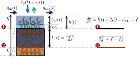
Figure 1: Hydrologic conceptual model where $q_{\mathrm{in}}$ and $q_{\mathrm{out}}$ are inflows and outflows, $i_{\mathrm{p}}$ is the rainfall intensity, $e_{\mathrm{TR}}$ is the real evapotranspiration, $f$ is the infiltration rate, $f_{\mathrm{g}}$ is the groundwater replenishing, $\psi$ is the suction head acting at the wetting front, $\Delta\theta$ is the soil moisture deficit, $h_{\mathrm{ef}}$ is the effective water depth while $h$ is the total depth, $h_{\mathrm{0}}$ are the losses through plant interception and initial abstractions, $L(t)$ is the effective depth of the saturated zone, and $f_{\mathrm{d}}$ is the cumulative infiltrated depth. Two fundamental equations are solved for the atmosphere-soil interface and the wetting front-soil interface.

2.1.1 Mass Balance Equation

The overall mass balance differential equation is written for all cells of the domain, and accounts for the surface and the groundwater replenishing mass balance as follows (see Fig. 1):

$$\frac{\partial\bm{h}_{\mathrm{ef}}(t)}{\partial t} ={\bm{q}_{\mathrm{in}}}(t)-{\bm{q}_{\mathrm{out}}}(t)+\bm{i}_{\mathrm{p}}(t)-\bm{e}_{\mathrm{TR}}(t)-\bm{f}(t)$$ (1a)

$$\frac{\partial\bm{f}_{\mathrm{d}}(t)}{\partial t} =\bm{f}(t)-\bm{f}_{\mathrm{g}},$$ (1b)

where $q_{\mathrm{in}}$ and $q_{\mathrm{out}}$ are the inflow and outflow rates, respectively, $i_{\mathrm{p}}$ is the rainfall rate, $e_{\mathrm{TR}}$ is the evapotranspiration rate, $q_{\mathrm{out}}$ is the outflow rate, $f$ is the infiltration rate, and $f_{\mathrm{g}}$ is the groundwater replenishing rate.

The water balance in the watershed cells is calculated from inflows, outflows, rainfall, evapotranspiration, and infiltration. Using a finite-difference forward Eulerian scheme, we discretize the mass balance into:

$$\bm{h}_{\mathrm{ef}}(k+1) =\bm{h}_{\mathrm{ef}}(k)+\Delta t\Bigl{(}\bm{q}_{\mathrm{in}}(k)+\bm{i}_{\mathrm{p}}(k)-\bm{e}_{\mathrm{TR}}(k)-\bm{q}_{\mathrm{out}}(k)-\bm{f}(k)\Bigr{)}$$ (2a)

$$\bm{f}_{\mathrm{d}}(k+1) =\bm{f}_{\mathrm{d}}(k)+\Delta t\Bigl{(}\bm{f}(k)-\bm{f}_{\mathrm{g}}\Bigr{)},$$ (2b)

where $\Delta t$ = model time-step, $k$ = time-step index, $\bm{h}_{\mathrm{ef}}$ = effective water depth, $\bm{q}_{\mathrm{in}}$ = summation of inflows for all directions, $\bm{i}_{\mathrm{p}}$ = rainfall intensity, $\bm{e}_{\mathrm{TR}}$ = evapotranspiration rate, $\bm{q}_{\mathrm{out}}$ = summation of outflows for all directions, $\bm{f}$ = infiltration rate, and $\bm{f}_{\mathrm{g}}$ = sub-surface exfiltration rate, with all vectors $\in\mathbb{\bm{R}}^{\mathrm{q}}$ and with $q$ being the number of cells in the domain. The full derivation of the hydrological inputs, such as Evapotranspiration, Green-Ampt (Green and Ampt, 1911) infiltration modeling, and groundwater replenishment rate, is described in Supplemental Information (SI).

To solve Eq. (2a), we calculate $\bm{q}_{\mathrm{in}}$ and $\bm{q}_{\mathrm{out}}$ from a momentum equation. Herein, we use Manning’s equation coupled with the non-linear reservoir method to allow modeling of losses to initial abstraction, such that:

$$q_{\mathrm{x}}^{\mathrm{i,j}}=\frac{\max\Bigr{(}{h^{\mathrm{i,j}}_{\mathrm{ef}}-h_{0}^{\mathrm{i,j}},0}\Bigr{)}^{5/3}}{n^{\mathrm{i,j}}}\left(s^{\mathrm{i,j}}_{\mathrm{f}}\right)^{1/2}\Delta y$$ (3a)

$$q_{\mathrm{y}}^{\mathrm{i,j}}=\frac{\max\Bigr{(}{h^{\mathrm{i,j}}_{\mathrm{ef}}-h_{0}^{\mathrm{i,j}},0}\Bigr{)}^{5/3}}{n^{\mathrm{i,j}}}\left(s^{\mathrm{i,j}}_{\mathrm{f}}\right)^{1/2}\Delta x$$ (3b)

where $h_{0}$ is the initial abstraction, $\bm{s}_{\bm{\mathrm{f}}}$ is the friction slope, assumed as the bottom slope, $n$ is the Manning’s roughness coefficient in ($\mathrm{s\cdot m^{-1/3}}$), $\Delta x$ is the pixel $x$ dimension, and $\Delta y$ is the pixel $y$ dimension.

From the previous equation, it is observed that the hydraulic radius is assumed to be the effective depth of the water ($h-h_{0}$), which is more accepted if there are relatively smaller depths and larger grid dimensions (Akan and Iyer, 2021). The friction slopes used in Eq. (3) must be positive and directed toward the downstream cell of the central cell, assuming that all cells have an assigned flow direction.

The mass balance equation shown in Eq. (2a) requires the calculation of intercell flows and a flow direction matrix for the $x-x$ and $y-y$ directions. The flow direction matrix $\bm{B}_{\mathrm{d}}^{\mathrm{w}}$ can be calculated with the common flow-direction algorithms found in Geographic information systems (GIS) such as ArcGIS or QGIS. Here, we applied these algorithms in Matlab (Greenlee, 1987). Moreover, instead of creating large matrices with only a few values, we create sparse matrices to store only the flow direction information, reducing storage and allowing the model scalability for highly detailed resolutions. The net-flux, herein defined as the difference between inflows and outflows, is expressed as follows:

$$\bm{q}_{\mathrm{in}}(k)-\bm{q}_{\mathrm{out}}(k)=\bm{B}_{\mathrm{d}}^{\mathrm{x-x}}(k)\bm{q}^{\mathrm{x-x}}_{\mathrm{out}}(k)+\bm{B}_{\mathrm{d}}^{\mathrm{y-y}}(k)\bm{q}^{\mathrm{y-y}}_{\mathrm{out}}(k)+\bm{q}_{\mathrm{s}}(k),$$ (4)

where $\bm{B}_{\mathrm{d}}\in\mathbb{R}^{\mathrm{q}\times\mathrm{q}}$ is the direction matrix that contains the flow connection relationship between each cell for each direction $x$ or $y$. Note that these matrices can only have -1, 0 or 1 numbers to represent the flow topology. Eq. (4) is then introduced in Eq. (2a) to develop the watershed mass-balance and energy conservation dynamical system. The vector $\bm{q}_{\mathrm{s}}$ represents an internal boundary condition of source inflow hydrograph that can enter the cells of the domain.

The i-th row of $\bm{B}_{\mathrm{d}}^{\mathrm{x-x}}$ contains the information of the steepest downstream cell of $i$, for the $x$ direction, in terms of topographic elevation, which is derived from a treated digital elevation model. If the cell $i$ is a sink, the maximum slope would be negative and the i-th row would be zero, resulting in a failed 2-D kinematic wave model. Therefore, we first perform a pre-processing in the DEM. To this end, we filter sinks and noises with 3 algorithms: the $\mathtt{fillsinks}$ and the $\mathtt{imposemin}$, both available in topotoolbox algorithms (Schwanghart and Scherler, 2014) and we also use the $\mathtt{DTMfilter}$, available in QGIS (Vosselman, 2000). These algorithms allow filling the sinks and imposing minimum slopes such that both kinematic-wave and diffusive-wave models can be used and compared.

The inputs $\bm{i}_{\mathrm{p}}(k)$, and $\bm{e}_{\mathrm{TR}}(k)$ can be assumed to be space- and time-variant or invariant internal boundary conditions, while $\bm{f}(k)$ (i.e., the infiltration rate) is a function of state $\bm{h}_{\mathrm{ef}}(k)$ and the accumulated infiltration depth $\bm{f}_{\mathrm{d}}$. Details of how infiltration is calculated can be found in (Gomes Júnior et al., 2022). Another important consideration is the extraction of the reservoir area in the effective calculation of the inflow hydrograph in the reservoir.

To avoid considering precipitation twice in the reservoir water balance (i.e., if the watershed contains the reservoir, then the reservoir would be considered twice in the calculations), we subtract an instantaneous rate ($i_{\mathrm{p}}\times A_{\mathrm{max}}$, with $A_{\mathrm{max}}=$ reservoir maximum area) from the inflow hydrograph to neglect the effect of rainfall in the reservoir area.

2.1.2 Adaptive Time-step

During high transient periods, the flood wave propagation is intense, resulting in relatively higher velocities. Therefore, the model stability can be affected if coarse fixed time-steps are used. To this end, we employ an adaptive time-step numerical approach to ensure modeling numerical stability by guaranteeing a Courant-Friedrichs-Levy (CFL) (Courant et al., 1928) number below a certain threshold as follows:

$$\Delta t(k+1)=\min{\Bigl{(}\alpha\overbrace{\frac{\Delta x}{\max{(\bm{v}(k))}}}^{\mathrm{CFL}},\Delta t_{\mathrm{max}}\Bigr{)}},$$ (5)

where $\alpha<1$ is a decreasing factor in the CFL, $\Delta x$ is the cell spatial resolution, and $\bm{v}$ is the velocity in all cells solved by $\bm{v}(k)=(\bm{q}_{\mathrm{out}}\Delta x)\oslash(\bm{h}_{\mathrm{ef}}(k))$ and $\Delta t_{\mathrm{max}}$ is the maximum time-step of the simulation.

2.2 Reservoir Model

The reservoir receives inflow from the watershed, which can be calculated by solving Eq. (3) for the outlet cell $\bm{i}_{0}$. Therefore, the reservoir net inflow can be calculated as:

$$q_{\mathrm{in}}^{\mathrm{r}}(k)=q_{\mathrm{out}}^{w}(k)+\Bigl{(}i_{\mathrm{p}}^{\mathrm{r}}(k)-e_{\mathrm{p}}^{\mathrm{r}}(k)\Bigr{)}\omega_{\mathrm{r}}(k)$$ (6)

where $q_{\mathrm{out}}^{w}$ is the watershed outflow, $i_{\mathrm{p}}^{\mathrm{r}}$ is the rainfall intensity in the reservoir, $e_{\mathrm{p}}^{\mathrm{r}}$ is the evaporation, and $\omega_{\mathrm{r}}:=f(h^{\mathrm{r}}(k))$ is the depth-varying reservoir area.

The derivation of $\omega_{\mathrm{r}}$ is made from known stage x area values. A continuous function of the reservoir area in terms of water depth is built for each known stage x area value. A detailed explanation and mathematical derivation of this procedure is shown in the SI. For simplicity of notation, we assume $\omega_{\mathrm{r}}(h)=\omega_{\mathrm{r}}$ and $\eta(h)=\eta$.

By solving a mass balance equation (7) and an energy equation (8), we can determine the reservoir outflow as follows (Gomes Júnior et al., 2022):

$$h^{\mathrm{r}}(k+1)=h^{\mathrm{r}}(k)+\Bigl{(}\frac{\Delta t}{\omega^{\mathrm{r}}\eta}\Bigl{)}\left(q_{\mathrm{\mathrm{in}}}^{\mathrm{r}}(k)-q_{\mathrm{out}}^{\mathrm{r}}(k)\right),$$ (7)

$$q_{\text{out }}^{\mathrm{r}}\left(h^{\mathrm{r}}(k),u_{\mathrm{v}}(k),u_{\mathrm{s}}(k)\right)=\left\{\begin{array}[]{l}u_{\mathrm{v}}(k)k_{\mathrm{o}}\Bigl{(}\widehat{h}^{\mathrm{r}}_{\mathrm{v}}(k)\Bigr{)}^{\alpha_{\mathrm{v}}}\text{ if }h^{\mathrm{r}}(k)\leq p,\quad\text{ else }\\ u_{\mathrm{v}}(k)k_{\mathrm{o}}\Bigl{(}\widehat{h}^{\mathrm{r}}_{\mathrm{v}}(k)\Bigr{)}^{\alpha_{\mathrm{v}}}+u_{\mathrm{s}}(k)k_{\mathrm{s}}\Bigl{(}\widehat{h}^{\mathrm{r}}_{\mathrm{s}}(k)\Bigr{)}^{\alpha_{\mathrm{s}}}\end{array}\right.$$ (8)

where $k_{\mathrm{o}}$ and $k_{\mathrm{s}}$ are the orifice and spillway linear rating-curve coefficients, $\alpha_{\mathrm{o}}$ and $\alpha_{\mathrm{s}}$ are the exponents of these rating-curves. The variable $\widehat{h}^{\mathrm{r}}_{\mathrm{v}}\left(h^{\mathrm{r}}(k)\right)=\max\left(h^{\mathrm{r}}(k)-\left(h_{0}+h_{\mathrm{m}}\right),0\right)$, is the effective water depth at the orifice, $h_{0}$ is orifice depth from the bottom, $h_{m}=0.2d_{h}$, $d_{h}$ is the hydraulic diameter of the orifice, $\widehat{h}^{\mathrm{r}}_{\mathrm{s}}\left(h^{\mathrm{r}}(k)\right)=\max(h^{\mathrm{r}}(k)-p,0)$, is the effective water depth at the gate, where $p$ is the spillway elevation, $\omega^{\mathrm{r}}:=f\left(h^{\mathrm{r}}(k)\right)$ is the reservoir stage-area function, $u_{\mathrm{v}}$ is the valve openness and $u_{\mathrm{s}}$ is the gate openness.

By calculating the Jacobians of Eq. (8), we can derive a linearized model for the reservoir outflow that considers control in valves and gates by performing a Taylor’s series 1st order approximation. Let $\alpha(k)$ be the Jacobian of Eq. (8) with respect to $h^{\mathrm{r}}$, $\beta(k)$ the Jacobian with respect to $u_{\mathrm{v}}$, and $\gamma(k)$ the Jacobian with respect to $u_{\mathrm{s}}$, presented as follows:

$$\overbrace{\frac{\partial q_{\mathrm{out}}^{\mathrm{r}}\left(h^{\mathrm{r}}(k),u_{\mathrm{v}}(k),u_{\mathrm{s}}(k)\right)}{\partial h^{\mathrm{r}}}}^{\alpha(k)} =\alpha_{\mathrm{v}}u_{\mathrm{v}}k_{\mathrm{o}}\Bigl{(}\widehat{h}_{\mathrm{v}}(k)\Bigr{)}^{\alpha_{\mathrm{v}}-1}+\alpha_{\mathrm{s}}u_{\mathrm{s}}(k)k_{\mathrm{s}}\Bigl{(}\widehat{h}_{\mathrm{s}}(k)\Bigr{)}^{\alpha_{\mathrm{s}}-1}$$ (9a)

$$\overbrace{\frac{\partial q_{\mathrm{out}}^{\mathrm{r}}\left(h^{\mathrm{r}}(k),u_{\mathrm{v}}(k)\right)}{\partial u_{\mathrm{v}}}}^{\beta(k)} =k_{\mathrm{o}}\Bigl{(}\widehat{h}_{\mathrm{v}}(k)\Bigr{)}^{\alpha_{\mathrm{v}}}$$ (9b)

$$\overbrace{\frac{\partial q_{\mathrm{out}}^{\mathrm{r}}\left(h^{\mathrm{r}}(k),u_{\mathrm{s}}(k)\right)}{\partial u_{\mathrm{s}}}}^{\gamma(k)} =k_{\mathrm{o}}\Bigl{(}\widehat{h}_{\mathrm{s}}(k)\Bigr{)}^{\alpha_{\mathrm{s}}},$$ (9c)

which ultimately turns out in a linearized model around an equilibrium point $\bm{x}_{\mathrm{eq}}=[h^{\mathrm{r}}_{*},u_{\mathrm{v}}^{*},u_{\mathrm{s}}^{*}]^{\mathrm{T}}$ that collects the reservoir depth, valve and gate openness as follows:

$$q_{\mathrm{out}}^{\mathrm{r}}\left(h^{\mathrm{r}}(k),\bm{x}_{eq}\right) =\overbrace{q_{\mathrm{out}}^{\mathrm{r}}\left(h_{*}^{\mathrm{r}}\right)}^{\epsilon(k)}+\overbrace{\left.\alpha\right|_{h^{\mathrm{r}}=h_{*}^{\mathrm{r}},u_{\mathrm{v}}=u_{\mathrm{v}}^{*},u_{\mathrm{s}}=u_{\mathrm{s}}^{*}}}^{\tilde{\alpha}(k)}\left(h^{\mathrm{r}}(k)-h_{*}^{\mathrm{r}}\right)$$ (10)

$$+\overbrace{\left.\beta\right|_{h^{\mathrm{r}}=h_{*}^{\mathrm{r}},u_{\mathrm{v}}=u_{\mathrm{v}}^{*}}}^{\tilde{\beta}(k)}\left(u_{\mathrm{v}}(k)-u_{\mathrm{v}}^{*}\right)+\overbrace{\left.\beta\right|_{h^{\mathrm{r}}=h_{*}^{\mathrm{r}},u_{\mathrm{v}}=u_{\mathrm{v}}^{*}}}^{\tilde{\gamma}(k)}\left(u_{\mathrm{s}}(k)-u_{\mathrm{s}}^{*}\right),$$

where the orifice is defined by parameters $k_{\mathrm{o}}$ and $\alpha_{\mathrm{v}}$ and the gate is described by $k_{\mathrm{s}}$ and $\alpha_{\mathrm{s}}$.

Therefore, tunning the orifice and gate parameters with different values allow the model to simulate rectangular, circular, or variable shape orifices while gates can be modeled as open spillways (i.e., Thompson Spillway $\alpha_{\mathrm{s}}=3/2$) or as controllable gates simulated as orifices (i.e., $\alpha_{\mathrm{s}}=1/2$). The linear parameters $k_{\mathrm{o}}$ and $k_{\mathrm{s}}$ are the multiplication of all linear terms and terms inside exponential equations that are not a function of the representative water depth in the hydraulic equations. For the orifice case, $k_{\mathrm{o}}=c_{d}a_{ef}\sqrt{2g}$, where $c_{d}$ is the orifice discharge coefficient, $a_{ef}$ is the orifice area, and $g$ is the gravity acceleration. More details on the modeling of the governing coefficients can be found in (Gomes Júnior et al., 2022; French and French, 1985).

Substituting the inflow discharge from the watershed [Eq. (6)] which is an input data for the reservoir model derived from the watershed model, the linearized outflow discharge [Eq. (10)] derived from Eqs. (8) and (9), and tracking the outflow discharge as the output of the reservoir model, we develop a reservoir state-space model, such that:

$$\begin{bmatrix}h^{\mathrm{r}}(k+1)\\ q_{\mathrm{out}}^{\mathrm{r}}(k)\end{bmatrix}=\begin{bmatrix}A(k)\\ C(k)\end{bmatrix}h^{\mathrm{r}}(k)+\begin{bmatrix}B^{\mathrm{v}}(k)\\ D^{\mathrm{v}}(k)\end{bmatrix}u_{\mathrm{v}}(k)+\begin{bmatrix}B^{\mathrm{s}}(k)\\ D^{\mathrm{s}}(k)\end{bmatrix}u_{\mathrm{s}}(k)+\begin{bmatrix}\phi(\bm{x}_{\mathrm{eq}}(k))\\ \epsilon(\bm{x}_{\mathrm{eq}}(k))\end{bmatrix}$$ (11)

where the tracked state is the reservoir water depth $(h^{\mathrm{r}}(k))$ and the output is the reservoir outlet discharge $(q_{\mathrm{out}}^{\mathrm{r}})$ being controlled by the valve ($u_{\mathrm{v}}$) and gate ($u_{\mathrm{s}}$) openings. The first row represents a mass balance equation, whereas the second row is an energy balance equation. Time-varying single matrices $A(k)$, $B^{\mathrm{v}}(k)$, $B^{\mathrm{s}}(k)$, $C^{\mathrm{v}}(k)$, $C^{\mathrm{s}}(k)$, $D^{\mathrm{v}}(k)$, $D^{\mathrm{s}}(k)$ are derived taken the linear terms of $h^{\mathrm{r}}$ or $u_{\mathrm{v}}$, or $u_{\mathrm{s}}$ from Eqs.  (7) and (8). The source and linearized terms $\phi(k)$ collects the inflow discharge from the watershed and the results of substitution of the operational point into the linearized outflow discharge equation in Eq. (8). Similarly, $\epsilon(k)$ collects the applying of the operational point into the linearized terms of the discharge, in Eq. (8).

The previous derivation of of the state-space model in Eq. (11) can be easily expanded to more reservoirs and watersheds using topological relationships (Gomes Júnior et al., 2022).

2.3 Model Predictive Control

2.3.1 Objective Function

The operation of stormwater reservoirs can have multiple goals. For flood control, reservoirs should be operated to mitigate peak flows. One way to attenuate peak flow using active control techniques is to transform the reservoir operation into a minimization of flood costs (Gomes Júnior et al., 2022). Flood costs can be either the cost of flood damage or can be abstracted to include various flood-related costs such as (i) valve operation (i.e., control energy), (ii) maximum water level at the reservoir, or (iii) violation of maximum tolerable outflow. These objectives can be grouped into a single-objective function given by:

$$\min_{\bm{u}_{\mathrm{v,k}},\bm{u}_{\mathrm{s,k}}}\sum_{k=0}^{N_{\mathrm{p}}-1} \bm{J}\Bigl{(}\bm{h}^{\mathrm{r}}(k+1),\bm{u_{\mathrm{v}}}(k+1),\bm{u_{\mathrm{s}}}(k+1)\Bigr{)}=\rho_{\mathrm{u}}\left\|\Delta\bm{u}_{\mathrm{v,k}}^{\mathrm{T}}\right\|_{2}^{2}+\rho_{\mathrm{u}}\left\|\Delta\bm{u}_{\mathrm{s,k}}^{\mathrm{T}}\right\|_{2}^{2}$$

$$+\rho_{r}\Bigl{(}\left\|\max{(\bm{h}^{\mathrm{r}}-h_{\mathrm{ref}}^{r},0)}\right\|_{\infty}\Bigr{)}+\rho_{\mathrm{q},\mathrm{k}}\left(\left\|\max\left(\bm{q}_{\mathrm{k}}^{\mathrm{r}}-{q}^{\mathrm{r}}_{\mathrm{ref},\mathrm{k}},0\right)\right\|_{\infty}\right)$$

$$+\rho_{**}\Bigl{(}\left\|\max{(\bm{q}_{k}^{\mathrm{r}}-q_{max}^{**},0)}\right\|_{\infty}\Bigr{)},$$ (12)

where $\bm{J}$ is the cost function and their weights are given for the control input $(\rho_{\mathrm{u}})$, for the depths of the surface of the water in the reservoirs $(\rho_{\mathrm{r}})$ and for the exceedance of the maximum tolerable flow $(\rho_{\mathrm{q}})$. $N_{\mathrm{p}}$ is the prediction horizon, $\Delta\bm{u}_{\mathrm{v,k}}=[\Delta u_{\mathrm{v,1}}\dots\Delta u_{\mathrm{v,N_{{p-1}}}}]^{\mathrm{T}}$, $\Delta\bm{u}_{\mathrm{s,k}}=[\Delta u_{s,1}\dots\Delta u_{\mathrm{s,N}_{\mathrm{p-1}}}]^{\mathrm{T}}$$,\bm{h}_{\mathrm{k}}^{\mathrm{r}}=[h^{\mathrm{r}}_{\mathrm{1}},\dots h^{\mathrm{r}}_{\mathrm{N_{\mathrm{p}}-1}}]^{\mathrm{T}}$, $\bm{q}^{\mathrm{r}}=[q_{\mathrm{out,1}}^{\mathrm{r}},\dots q_{\mathrm{out,N_{\mathrm{p}}-1}}^{\mathrm{r}}]^{\mathrm{T}}$, $\bm{q}_{\mathrm{ref}}^{\mathrm{r}}$(k) is the time-varying reference outflow.

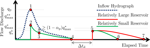
Figure 2: Inflow and outflow hydrographs of a relatively large and a relatively small stormwater reservoir with water quantity and quality control, where $\Delta t_{\mathrm{d}}$ is the required detention time. The factor $\alpha_{\mathrm{p}}$ can be tuned and be used to represent a desired peak flow reduction under minor flood events with maximum predicted inflows smaller or equal than $q_{\mathrm{max}}^{*}$. The relatively large reservoir can store all inflow hydrograph and later release after a detention time threshold is reached, while the relatively small reservoir do not have the storage capacity to do and has to be operated focusing on flood mitigation.

The problem constraints are given by the physics of the system dynamics, and the control signals $\bm{u}_{\mathrm{k}}$ have each entry between 0 and 1, such that the valves can only be fully or partially opened. Therefore, the solution of the minimization function of Eq. (2.3.1) is mathematically contrained by:

s.t. $$\mathrm{Eq.}~{}\eqref{equ:state_space}$$ (13a)

$$\Delta{}u_{\mathrm{min}}\leq{}\Delta u\left(k\right)\leq\Delta{}u_{\mathrm{max}}$$ (13b)

$$\bm{u}_{\mathrm{v}}(k),\bm{u}_{\mathrm{s}}(k)\in{}\mathcal{\bm{U}}:=\mathbb{R}\in[0,1]$$ (13c)

$$\bm{h}^{\mathrm{r}}(k)\in{}\mathcal{\bm{X}}:=\mathbb{R}\in[0,h^{\mathrm{r}}_{\mathrm{max}}]$$ (13d)

where $h^{\mathrm{r}}_{\mathrm{max}}$ is the maximum reservoir depth.

The reference outflow $q_{\mathrm{ref}}^{\mathrm{r}}(k)$ represents the operational tolerable flow. In this paper, we develop a heuristic approach to change the reference outflow according to the maximum inflow ($\bm{q}_{\mathrm{in,k}}^{\mathrm{r}}$) predicted in the control horizon $k$. The goal is to define a control that could work not only for large storms, but also for minor events. The reference $\bm{q}_{\mathrm{ref}}^{\mathrm{r}}$ changes according to the predicted inflows and can be written as:

$$\bm{q}_{\mathrm{ref,k}}^{\mathrm{r}} =\begin{cases}\alpha_{\mathrm{p}}\max{(\bm{q}_{\mathrm{in,k}}^{\mathrm{r}})},~{}\text{if $\max{(\bm{q}_{\mathrm{in,k}}^{\mathrm{r}})}\leq q_{\mathrm{max}}^{*}$}\\ q_{\mathrm{max}}^{*},~{}\text{Elsewhere}\\ \end{cases}$$ (14a)

$$\rho_{\mathrm{q,k}} =\begin{cases}10^{1}\rho_{\mathrm{u}},~{}\text{if $\max{(\bm{q}_{\mathrm{in,k}}^{\mathrm{r}})}\leq q_{\mathrm{max}}^{*}$}\\ 10^{2}\rho_{\mathrm{u}},~{}\text{Elsewhere}\\ \end{cases}$$ (14b)

$$\rho_{**} =\begin{cases}10^{3}\rho_{\mathrm{u}},~{}\text{if }\max{(\bm{q}_{\mathrm{in,k}}^{\mathrm{r}})\geq q_{\mathrm{max}}^{**}}\\ 0,~{}\text{Elsewhere}\end{cases}$$ (14c)

where $\alpha_{\mathrm{p}}$ represents the tolerable maximum reservoir outflow peak / maximum inflow from the upstream catchment at the control horizon. In other words, ($1-\alpha_{\mathrm{p}}$) represents the minimum peak flow reduction goal applied only in cases where the maximum predicted inflow on the control horizon is smaller than $q_{\mathrm{max}}^{**}$. If the predicted maximum inflow is greater than $q_{\mathrm{max}}^{**}$, we assume that this is a large event and limit the maximum outflow to $q_{\mathrm{max}}^{**}$ instead of trying to reduce only a percentage of the maximum flow. An illustrative example of the maximum flows predicted in a prediction horizon is shown in Fig. 3.

The aforementioned parameters are defined according to the reservoir goals and can be parametrized for different reservoirs, watersheds, and local regulations of maximum outflows. Posing these constraints and details, the problem is formulated as a non-linear, non-convex optimization problem. In this model we have implemented two solvers for the solution of Eq. (2.3.1), the $\mathtt{patternsearch}$ and the $\mathtt{fmincon}$ solvers. Here we use the $\mathtt{fmincon}$ algorithm from Matlab. Previous modeling results using $\mathtt{globalsearch}$ and $\mathtt{genetic~{}algorithms}$ resulted in overly expensive time solutions and were not utilized in this investigation.

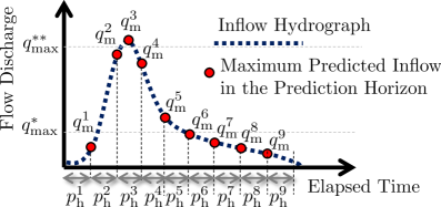
Figure 3: Inflow hydrograph and the definition of the maximum inflow $q_{\mathrm{m}}$ for each prediction horizon $p_{\mathrm{h}}$. The weights to be used in Eq. (2.3.1) are defined by each maximum inflow $q_{m}$ for each prediction horizon as shown in Eq. (14). Therefore, the control theoretical goal is changed according to the predicted flood magnitude. Note that $q_{\mathrm{m}}^{3}$ violates the threshold for large flood $q_{\mathrm{max}}^{**}$, increasing the focus of the control for flood mitigation, while $q_{\mathrm{max}}^{1}$, for example, has a maxium predicted inflow in the prediction horizon smaller than the threshold for minor floods.

Instead of starting the optimization with randomly multi-start points focusing on finding global minima, we created initial points based on simple ruled-based logic. The rationale behind is to start with initial points with no valve operation (i.e., no control effort) but that would explore the whole decision space. Given a number of random inputs ($n_{\mathrm{r}}$) for the multi-start search, we create a series of inputs $\bm{U}_{\mathrm{0,k}}=[\bm{u}_{0}^{1},\dots\bm{u}_{0}^{n_{\mathrm{r}}}]^{\mathrm{T}}$, with $\bm{u}_{0}^{i}=\frac{i}{n_{\mathrm{r}}}[\bm{1}_{N_{\mathrm{p}}\times 1}]~{}\forall~{}i\in[1,n_{\mathrm{r}}]\in\mathbb{N_{++}}$ and run the optimization problem for each of them. Afterwards, we choose only the solution with a smaller objective function value, given by Eq. (2.3.1).

Finally, to accomplish proxy water quality goals (i.e., increase detention time), we create a routine that identifies the maximum inflow in the prediction horizon, and if this quantity equals 0, we start counting the detention time. At the beginning of this phase, we close the valves (that is, $u_{\mathrm{v}}(k)=0$) and if no other event occurs during a maximum detention time period ($\Delta t_{\mathrm{d}}$), we release the outflow by opening the valves at a capacity equal to $q_{\mathrm{t}}^{*}$. This can be the threshold for minor flood events or can also be tuned as a flow used to avoid erosion, for example. By limiting the outflow to $q_{\mathrm{t}}^{*}$, the valve opening can be calculated as:

$$u_{\mathrm{r}}=\min{\Bigr{(}\frac{q_{\mathrm{t}}^{*}}{k_{\mathrm{o}}\sqrt{h_{\mathrm{r}}^{e}}},1\Bigr{)}},$$ (15)

where $k_{\mathrm{o}}=c_{\mathrm{d}}a_{\mathrm{ef}}\sqrt{2g}$ is the orifice coefficient, $c_{\mathrm{d}}$ is the discharge coefficient, $a_{\mathrm{ef}}$ is the effective area of the orifice, $g$ is the acceleration of gravity and $h_{\mathrm{r}}^{\mathrm{e}}$ is the reservoir water depth at the end of the detention time.

During wet weather periods, that is, periods where the inflow is smaller than a pre-defined flow threshold (i.e., typically $<2~{}\mathrm{m^{3}\cdot s^{-1}}$) during the prediction horizon, we stop the MPC algorithm and switch the problem to a fully water quality-based control. However, if some of the predicted inflows are positive, the algorithm returns to flood-based control by seeking the minimization of Eq. (2.3.1). This simple heuristic rule allows us to change the problem control from a flood-based control approach during wet weather events to a water quality-based control approach during dry weather periods while avoiding releasing high flows by limiting the valve opening up to a condition where a maximum flow released that is smaller than $q_{\mathrm{max}}^{*}$ is expected.

A conceptual example of two reservoirs receiving the same inflow hydrograph is shown in Fig. 2 to illustrate the idea of the MPC approach with proxy water quality control. In Fig. 2, each notable point is described as follows. Point 1 represents the maximum inflow peak discharge, which is larger than the threshold for large flood events $q_{\mathrm{max}}^{**}$. The smaller reservoir cannot hold the total inflow hydrograph volume and has to start to release flows in 2 to allow a desired peak flow mitigation in 3, that is, the maximum peak flow released in 3 follows the desired peak flow factor for minor floods $\alpha_{\mathrm{p}}$. This factor is tuned to allow peak flow mitigation under relatively small events, which is a drawback of passive reservoirs designed only for relatively large events and hence with relatively large orifices that cannot mitigate small inflow discharges. After the inflow hydrograph stops in 4, both reservoirs now have the orifice valves closed all, even though the relatively large reservoir was always with the valves closed, since it had enough capacity to store the hydrograph volume.

After reaching the detention time $\Delta t_{\mathrm{d}}$ with no predicted inflow hydrographs in this period, both reservoirs now open the valves releasing a maximum flow $q_{*}^{\mathrm{t}}$, also tuned to represent a desired outflow rate that can be designed to avoid erosion or regulate a minimum flow discharge. The smaller reservoir has a faster stage-area function, providing a larger variation in the depth with a relatively smaller variation in volume, which explains the faster release of the flow while the larger reservoir takes longer to release all flow hydrograph. Both cases show how the MPC approach designed in this paper can enhance flood dynamics.

2.3.2 Performance Indicators

To evaluate the performance of the MPC strategy, we compare active-controlled results with a baseline scenario corresponding to the passive scenario, that is, the spillway gate and the valve are fully open. To quantify peak flow mitigation, we derive duration curves corresponding to the frequency of discharges and depths, as well as by calculating the average flow discharges and the root mean squared water depths during a 1-yr of continuous simulation.

For water quality, we track the detention time and the released volume through the valve to calculate the average detention time and a proxy representation of the treated runoff volume as a function of the product between the runoff volume of the outflow and the detention time. In summary, the average detention time can be defined as the weighted average between the runoff volume released by the valve with the detention time associated with the release. The treated (i.e., the volume that passed through the bottom orifice) is given by:

$$V_{\mathrm{out}}(k)=\int_{0}^{k}q_{\mathrm{out}}^{\mathrm{r}}(t)\mathrm{dt}=\sum_{i=0}^{k}q_{\mathrm{out}}^{\mathrm{r}}(i)\Delta t$$ (16)

By calculating the product between the runoff volume and the detention time and dividing by the runoff volume, we can derive the average detention time calculated as:

$$\bar{\Delta t_{\mathrm{d}}}(k)=\frac{\sum_{i=0}^{k}q_{\mathrm{out}}^{\mathrm{r}}(i)\Delta t_{d}(i)}{V_{\mathrm{out}}(k)}$$ (17)

where $\bar{\Delta t_{\mathrm{d}}}(k)$ is the average detention time for step $k$.

The detention time is only tracked and updated when the prediction inflow hydrograph within the control horizon is null and the reservoir water depth is greater than $0.2d_{\mathrm{h}}$. In other words, the detention time is only calculated when no flows are predicted and the water depth is enough to begin to be released by the reservoir passively. In cases of predicting inflow hydrographs or with a water depth stored in the reservoir, the detention time is constantly updated. Following this idea, the treated volume $V_{\mathrm{out}}$ from Eq. (16) is also only calculated when these conditions are met.

2.4 Study Area

The Aricanduva-I watershed drains 4.7 km² from the headwaters of the Aricanduva River. Since the urbanization of the São Paulo city, this area has suffered many problems due to extreme hydrological events. A detention reservoir (on-line) responsible for storing $\mathrm{200,000~{}m^{3}}$ of stormwater runoff (normal capacity below the spillway) discharges through a rectangular orifice (1.0 m $\times$ 1.0 m) operated passively, that is, no orifice control is currently implemented. During large events, an emergency spillway can be used, which discharges the overflow directly into the downstream drainage system (de Hidráulica, 2020), as presented in Fig. 4.

In the following numerical case studies, we investigate how the performance of the system would change if the orifice and the spillway were controlled through active valves and gates. The digital elevation model collected from airborne LiDAR surveys available on the GeoSampa portal (PMSP, 2017) and the land use and land cover data were retrieved from the Dynamic World database, which classifies the entire world into eight main classes (Brown et al., 2022). Both information is presented in Fig. 5. To treat the DEM and enhance flow continuity and pathways, we performed a GIS pre-processing in the raw DEM data. Using the topotoolbox (Schwanghart and Scherler, 2014) we fill sinks, smooth streams, and impose minimum slopes using functions $\mathtt{fillsinks}$, $\mathtt{klargestconncomps}$, and $\mathtt{imposemin}$ (Schwanghart and Scherler, 2014). The watershed is mostly described by the headwaters of the Aricanduva River and therefore has a relatively steep average slope of approximately 20%, indicating that gravitational effects probably govern the hydrodynamics of the catchment. Additionally, this catchment does not have the influence of other upstream reservoirs that would play a role in water storage within the catchment.

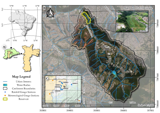
Figure 4: Study Area Map in São Paulo City - Brazil. The reservoir has an inlet channel and receives headwaters of Aricanduva watershed. During large events, runoff is spilled by a rectangular crest spillway.

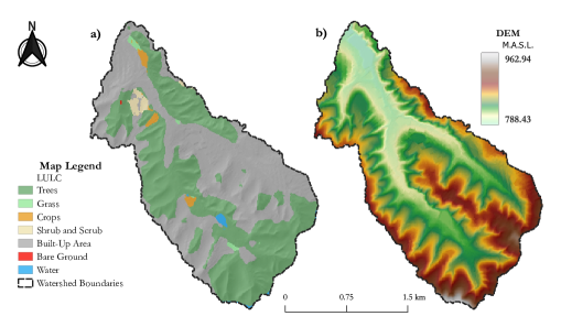
Figure 5: Land use and land cover map (a), hypsometric map of the watershed (b). Elevation was filled and resampled to $\mathrm{50~{}m}$. Following, D-8 watershed algorithm was run and the watershed boundary was created. All other maps were derived by clipping available rasters into this resulting polygon.

2.4.1 Watershed Properties

The soil Green-Ampt of suction head, saturated hydraulic conductivity, effective moisture content, and initial stored depth were estimated as 31.5 mm, 2.54 $\mathrm{cm\cdot h^{-1}}$, 0.476, and 5 mm, respectively (Rossman and Huber, 2016). The Manning’s roughness coefficient was estimated for each LULC of Fig. 5, resulting in 0.015, 0.06, 0.03, 0.12, 0.03, 0.05, and 0.016 $\mathrm{s\cdot m^{-1/3}}$ for Water, Trees, Grass, Crops, Shrub/Scrub, and Built Areas, respectively (Downer et al., 2006).

2.4.2 Reservoir Stage-Area-Volume

The reservoir has the area varying with the water surface depth and is described by points of depth x area, presented as follows:

$$A(h^{\mathrm{r}}(k))=\begin{cases}2,833.33h^{\mathrm{r}}(k)+50&\text{if $h^{\mathrm{r}}(k)\leq 0.9$}\\ 2,600+59,900(h^{\mathrm{r}}(k)-0.9)&\text{if $0.9\leq h^{\mathrm{r}}(k)\leq 1.9$}\\ 62,500+2,080(h^{\mathrm{r}}(k)-1.9)&\text{if $1.9\leq h^{\mathrm{r}}(k)\leq 4.4$}\\ 67,700+2,080(h^{\mathrm{r}}(k)-4.4)&\text{if $4.4\leq h^{\mathrm{r}}(k)\leq 6.9,$}\end{cases}$$ (18)

where the area values are given in m² and the depth values in m.

The depth-varying volume is calculated from the depth-area relationship by integrating this function in Matlab using the $\mathrm{integral}$ function. Between two known points of depth-area, we assume a linear variation of the area with respect to depth, allowing the analytical determination of the function that describes the area between two known depth-area points.

2.4.3 Outlet Devices

As previously mentioned, the reservoir has a $\mathrm{1~{}m\times 1~{}m}$ orifice located at the bottom and a spillway at the depth of $\mathrm{4.4~{}m}$ with 9 m of crest length. For the orifice, we assume a discharge coefficient of 0.61 resulting in $k_{\mathrm{o}}=5.4039$. If the spillway was uncontrolled (i.e., $q_{\mathrm{s}}(k)=k_{\mathrm{s}}(h(k)-p)^{1.5})$, the spillway coefficient would result in $k_{\mathrm{f}}=18.9$ (see Gomes Júnior et al. (2022)). However, if the spillway is retrofitted with a controllable asset that vertically changes the effective spillway area by a movable vertical gate (i.e., allowing the emergency spillway to work as an orifice), we can then use the orifice equation discharging at the atmosphere equation, such that:

$$q_{\mathrm{s}}(h)=c_{d}\overbrace{\Bigl{(}u_{\mathrm{s}}(k)l_{\mathrm{ef}}\Bigl{(}h(k)-p\Bigr{)}\Bigr{)}}^{a_{\mathrm{ef}}(k)}\sqrt{2g\Bigl{(}h(k)-p\Bigr{)}},$$ (19)

where $u_{\mathrm{s}}(k)$ is the control operation between 0 and 1, where 0 represents a fully closed gate and 1 represents a gate open a depth equals the effective depth in the gate $(h(k)-p)$. Equation (19) turns out in the format $q_{\mathrm{s}}=k_{\mathrm{s}}(h-p)^{\alpha_{s}}$ as follows:

$$q_{\mathrm{s}}(h)=\overbrace{c_{d}l_{\mathrm{ef}}\sqrt{2g}}^{k_{\mathrm{s}}}\Bigl{(}h(k)-p\Bigr{)}^{3/2},$$ (20)

with $\alpha_{\mathrm{s}}=3/2$.

Therefore, if we model the spillway as a controllable asset using an effective width of 9 m results in $k_{\mathrm{s}}=27$ and $\alpha_{\mathrm{s}}=3/2$ for a $c_{\mathrm{d}}=0.68$.

Although controlling the spillway may be desirable, a higher chance of overtopping can occur by reducing the spillway capacity during flood propagation. In cases where the predicted inflow supersedes the reservoir capacity volume, the model assumes the overtopping volume as the spillway outflow volume and emits an alert in the model that this condition is occurring. Typically, this condition would have a poor optimization function value by tunning the weights for exceeding $q_{\mathrm{max}}^{**}$ relatively high. This condition is more often to occur in poorly designed reservoirs.

A summary of the RTC-Stormwater model is presented in Fig. 6.

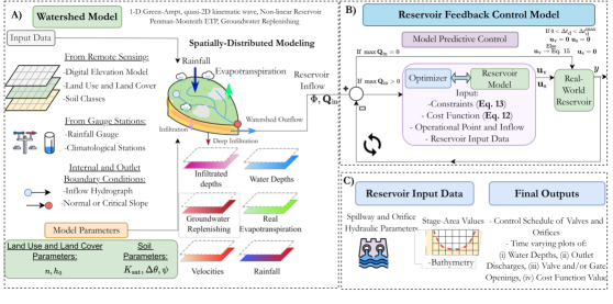
Figure 6: Summary of the modeling aspects of RTC-Stormwater. Part (A) is the watershed model that has raster input data that represent the topography, cover, and soils of the terrain. In addition, spatiallized climatologic inputs are considered to represent rainfall and input climatologic data to estimate potential evapotranspiration. Inflow and outlet boundary conditions can be parametrized. The autonomous watershed model results in time-varying rasters of infiltrated, surface water, rainfall, and evapotranspiration depths, in addition to flow velocities. Time-varying vectors of stage and discharge are also outputs of the model, and the latter are the input data for the Reservoir Feedback Control Model (B). The MPC feedback control is presented in Part (B) and the MPC is run considering the inflow hydrograph from the watershed, the cost function and constraints, the current operational points of the system, and the reservoir input data, which are shown in Part (C). Finally, the control schedule of the valve and gates to minimize the flood cost function, as well as time-varying plots of the states and outputs of the, are shown at the end of the simulation .

2.5 Numerical Case Study 1 - Comparing Kinematic Quasi-2D model with Full Momentum Model

In this numerical case study, our aim is to answer the following questions:

• Q1 - Does the model proposed here accurately simulate flow discharges for different pixel resolutions compaed to HEC-RAS 2D full momentum?

To this end, we applied the models in the study area catchment and compared the hydrographs generated at the outlet of the catchment. In this numerical case study, we neglect infiltration and initial abstraction, and we only assess the overland flow routing. Moreover, to test only the capacity of the model to predict flood depths, we consider a constant Manning’s roughness coefficient of $0.02~{}\mathrm{s\cdot m^{-1/3}}$.

The kinematic wave model is tested using the model described in this paper and is compared with the most advanced solver of HEC-RAS 6.3 - the Shallow-Water-Equation set solved with the Eulerian Method (SWE-EM Stricter Momentum) (Brunner, 2016). We tested the approach by modeling an unsteady-state rainfall of a 100-year storm with the Alternated Blocks hyetograph.

To make sure the reservoir storage effects do not affect the hydrographs results, we delineated an inter-catchment in HEC-RAS to represent the contributing storage areas that drain to the entry of the reservoir, as shown in Fig. 4. Therefore, the effective drainage area was reduced from 4.70 km² to 4.49 km².

All tested scenarios, in this numerical case study, were simulated with a constant time-step that varied according to each model to guarantee numerical stability. The hydrographs of the simulation are compared, and the peak and volume errors are calculated. We tested models with spatial resolutions of 10 and 30 m.

2.6 Numerical Case Study 2 - Simulating the Water Quantity and Quality Control Under Dynamic Rainfall Events

In this numerical case study, we focus on answering the following questions:

• Q2 - Is the water quantity and quality MPC algorithm presented in this paper capable of providing better control performance compared to the passive scenario (i.e., valves and gates always opened) under critical rainfall events?

• Q3 - Is the MPC algorithm capable of controlling floods while allowing a desired detention time?

To answer these questions, we applied the proposed model in the study area. In this numerical case study, the watershed was modeled with a cell size spatial resolution of 10 m. We tested a 44-hour event consisting of two design storms of 10-years, 2-hours duration, spanned 6-hours each other, as presented in Fig. 7. Both design storms have 77 mm of rainfall volume each and are temporally distributed using the Alternated Blocks method. This design event is chosen to show how the MPC strategy would work under relatively large events with rainfall events that occur sequentially, forcing the MPC strategy to perform under critical forecast storm events.

We compare the MPC approach with the passive scenario with valves always open. For the MPC algorithm, we assume a control interval of 1-h, a control horizon of 2-h, and a prediction horizon of 12-h. Furthermore, the MPC optimization function (2.3.1) is solved with the $\mathtt{fmincon}$ solver with 120 maximum function evaluations per each initial random initial guess of the solution. Therefore, assuming 5 initial points, the objective function is evaluated 600 times per control horizon, and the solution with a smaller cost function is chosen as the near-optimal control schedule of the prediction horizon. The objective function is evaluated by solving the reservoir dynamics for the prediction horizon and collecting the states to allow for a timely evaluation of the objective function. Therefore, it is important to have a relatively fast model.

The weights of Eq. (2.3.1) are assumed to represent typical detention pond goals. The detention time ($\Delta t_{\mathrm{d}}$) is assumed to be 18 hours to represent 1.5 prediction horizons of 12-hours and be a relatively sufficient time to sediment solids over the bottom of the detention pond. This parameter can also be adapted to local requirement conditions. In addition, even though the desired detention time is 18 hours, during inter-flood events the water quality focus might switch to flood control focus; therefore, not allowing the total desired detention time.

To measure the efficiency of the strategy, we plot the values of the objective function given by (2.3.1) and compute the minor and major flood times. These are defined as the duration of the reservoir outflow greater than $q_{\mathrm{max}}^{*}$ and $q_{\mathrm{max}}^{**}$, respectively.

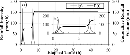
Figure 7: Hyetograph (a) and cumulative rainfall volume (b) for the example presented in Sec. 2.6, where $i(t)$ is the rainfall intensity and $P(t)$ is the cumulative rainfall volume. The rainfall event represent 2 design storms of 10-years, 2-hours, distributed with the Alternated Blocks Method, and spanned 6-hours each other. Each rainfall has 77 mm of volume and was determined using an IDF of Sao Paulo.

2.7 Numerical Case Study 3 - Simulating the Benefits of RTC under 1-year of Continuous Simulation with Spatial Rainfall and ETP

In this numerical case study, we aim to answer the following question.

• Q4 - What are the long term impacts of the MPC algorithm when used over a year of continuous simulation?

• Q5 - How does such control approach compare with passive scenarios of spillway always open with valves fully opened or partially opened with 75%, 50%, and 25% of the orifice area?

In this numerical case, we show a full implementation of the RTC strategy that couples a watershed model and a stormwater reservoir model predictive controller. We simulate the hydrologic and hydrodynamic processes in the watershed with sparse available rainfall and climatologic data, interpolating the data for all cells of the watershed. This numerical case study is an example of the implementation of the model developed in a real-world case study and for a continuous simulation.

We collect 10-min rainfall records from 7 rain gauge stations and daily climatologic inputs from 3 meteorological gauge stations as shown in Fig. 4c). The data are then interpolated and results are obtained so that each cell of the watershed domain has known interpolated rainfall and climatologic inputs. For reservoir control strategies, we compare static approaches of valve full opened (100%) with partial valve openings of 75%, 50%, and 25%, in addition to the MPC control.

2.7.1 Climatologic Inputs in the Watershed Model

The inputs for the quasi 2-D hydrodynamic model can be a combination of distributed or lumped assumptions. In this paper, we only assume rainfall and evapotranspiration as the climatologic inputs; however, other cases and more complex watersheds would require the implementation of inflow hydrographs as internal boundary conditions (Brunner, 2016). We perform an Inverse-Distance-Weightning interpolation (IDW) in the values of each station to estimate spatial values of rainfall and evapotranspiration over time. This procedure is fully detailed in the SI.

3 Results and Discussion

3.1 Numerical Case Study 1

The results of comparing RTC-Kinematic 2D with HEC-RAS 2D full momentum under an unsteady-state 100-yr storm temporally distributed with the Alternated Blocks method is presented in Fig. 8. An unsteady-state rainfall of 100-yr of return period often produces an event in which all terms of the SWE are required, such as local and convective acceleration (Akan and Iyer, 2021). Comparing a relatively simpler kinematic-wave model with the full-momentum unsteady state will probably present a scenario with a larger discrepancy between both models. Therefore, we test the model under the aforementioned conditions. The results presented in Fig. 8 show a relatively small error between both models, with both models with great visual agreement, especially for 10-m resolution.

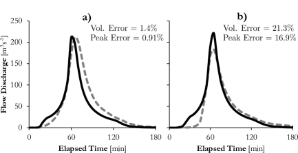
Figure 8: Comparison within the Kinematic-wave solution of the SWE with the full momentum solution. Black lines are the solution of HEC-RAS 2D and grey dashed lines are the RTC-Kinematic Wave solution. Part a) are results using a 10-m DEM resolution and b) are results with a 30-m resolution.

3.2 Numerical Case Study 2

The modeling results of the Numerical Case Study 2 are presented in Fig. 9. Part a) shows the inflow and outflow hydrographs for passive and active MPC controlled scenarios. The inflow hydrographs had peaks of approximately $\mathrm{148~{}m^{3}/s}$, resulting from two consecutive rainfall events of 2-hours and 10 years of recurrence interval. Although the passive scenario shows a great peak flow reduction for the first storm, the second peak flow was approximately $\mathrm{80~{}m^{3}/s}$ compared to $\mathrm{30~{}m^{3}/s}$ resulting from the MPC approach. The passive scenario provided 41% of peak flow reduction, while the MPC approach provided 79% attenuation.

The MPC approach scenario shows that reservoir outflows are smaller than $\mathrm{40~{}\mathrm{m^{3}/s}}$, that is, smaller than the defined threshold for large flood events $q_{\mathrm{max}}^{**}$ (see Fig. 2). The MPC approach predicts the future inflow hydrograph using a 12-hour time span, implements controls for each hour, and moves 2-hours in advance, receiving another forecast of the inflow hydrograph up to the total simulation time. Therefore, before the first inflow hydrograph peak, the MPC controller could predict the second and larger flow wave.

Although releasing flows greater than $q_{\mathrm{max}}^{*}$ would increase the costs associated with $\rho_{\mathrm{q,k}}$ from (2.3.1), by releasing flows at a rate smaller than $q_{\mathrm{max}}^{**}$, the method avoids a larger penalization from $\rho_{**}$. To this end, the MPC algorithm decides to release more flows after the first storm to have available volume and depth (i.e., potential energy) to actively control discharges and flood depths to the desired levels. We can see in Fig. 9b) that the active control decides to open the valves and gates during the inter-event duration to allow more future inflows can be stored in the reservoir and to be able to temporally partially close the gates and valves during the second inflow hydrograph to have a better flow mitigation. We can also see in Fig. 9c) that the MPC maintains the flow for approximately 18-hours and releases it afterward following (15). The cost functions for each scenario for each control horizon are presented in Fig. 9d), with optimization results of MPC significantly outperforming the passive scenario.

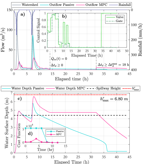
Figure 9: Results of the simulation presented in Numerical Case Study 2. Part a) is the discharges from the watershed and the outflows from the reservoir for the passive (i.e., gate and valve fully opened) and active scenario (i.e., MPC controlling valve and gate control schedule). Part b) shows the control schedule of orifice and gate opening derived from minimizing Eq. (2.3.1), where the control signal values represent the ratio between the controllable flow area with the available flow area. Part c) shows stage hydrographs in the reservoir for passive and active scenarios, and Part d) shows the objective function values of Eq. (2.3.1) for each prediction horizon. Variable $\Delta t_{\mathrm{d}}$ is the detention time and $\Delta t_{\mathrm{max}}$ is the required detention time.

3.3 Numerical Case Study 3

A summary of the watershed results is illustrated in Fig. 10. The cumulative values of rainfall, real evapotranspiration, and potential evapotranspiration are shown in parts (a)-(c) of this figure. A 1-year rainfall volume of approximately 1500 mm; a potential evapotranspiration of nearly 1150 mm and a real evapotranspiration of approximately 1000 mm are observed. Some areas had higher real evapotranspiration values due to water availability in the soil.

Fig. 10 part d) shows the 1-yr hyetograph and hydrograph, with details of the event of April 7 highlighted in part f) and a duration curve chart of rainfall and discharge shown in e). The hydrologic-hydrodynamic watershed modeling component of the model can be used as a tool to understand spatialized hydrologic information such as those presented in Fig. 10.

Using the 1-year watershed outlet hydrograph shown in Fig. 10 we set the MPC algorithm to optimize the valve and gate control while trying to control the detention time when no inflows are predicted. The MPC routine had a computational time of approximately 18 h to optimize the 4,380 control horizons of 2-hours for a 1 year of inflow hydrograph. The objective function was evaluated at least 2 million times, which shows the importance of having a fast cost function. The effects of how water quantity over water quality alters control decisions of the reservoir operation are discussed next.

The detailed event of April 7 (see Fig. 10f)) is expanded up to 11 April to show the performance of the MPC in comparison with other passive strategies, as shown with the outlet hydrographs for the scenarios with valves 100, 75, 50, and 25% opened in contrast to the MPC control in Fig. 11. Part (a) shows the inflow and outflow hydrographs, with all cases with peak flow reductions larger than 25 $\mathrm{m^{3}\cdot s^{-1}}$. Most of the controls, however, failed to mitigate the peak flows afterward the first two peaks. That means that the static operation of the reservoir did not have a peak flow mitigation effect for minor storms. On the other hand, the MPC control kept the water up to the expected detention time and then released it using the threshold for releasing the stored volume ($q_{\mathrm{t}}^{\mathrm{*}}$). The valve operation and water depth are shown in Fig. 11b) and Fig. 11c), respectively. These results imply that retrofitted reservoirs with active controlling capacity can not only mitigate large storms, but also minor storms. Furthermore, the results show that passive reservoirs usually cannot control smaller storms because they are designed for critical conditions of design storms with relatively long return periods.

In Fig. 11c), the stage hydrographs in the reservoir are depicted. It is noted that the MPC approach held more water inside the reservoir longer after reaching the first two peaks, since the optimization problem changed from flood to water quality control. Additionally, a valve opening larger than 25% seems to have minor mitigation effects for the minor upcoming floods.

Fig. 12 shows the evolution of the treated volume, which is only calculated when no inflow hydrographs are predicted on the control horizon and when the water depth is larger than a minimum threshold. More volume is treated using a valve opening of 25% compared to MPC; however, as shown in Fig. 13, the MPC approach has a longer detention time, which is a proxy representation of the water quality state of the system. The duration curves of the flow discharges and depths are shown in Fig. 14, indicating the probability of reaching a flow or depth larger than a threshold. It is observed from Fig. 14a) that the passive scenario has a sharp change in the flow duration curve after 2%. The stage duration curve on Fig. 14b) shows great variability in the probabilities of exceeding certain depths for the control strategies, with the MPC scenario presenting larger depths than the other controls.

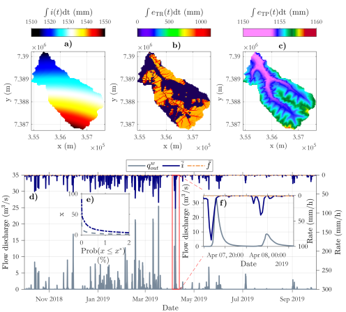
Figure 10: Rainfall ETP and ETR for the hydrologic year of 2018-2019 in the Aricanduva Catchment, Sao Paulo.

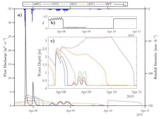
Figure 11: Example of a simple performance evaluation for a rainfall event using static rules of valve partially open with valve openness of 100, 75, 50, and 25% in comparison with the MPC controlled valve. Part (a) are the reservoir outlet hydrographs and the inflow hydrograph, while (b) is the control schedule of the MPC approach for this event, and (c) is the stage hydrograph in the reservoir.

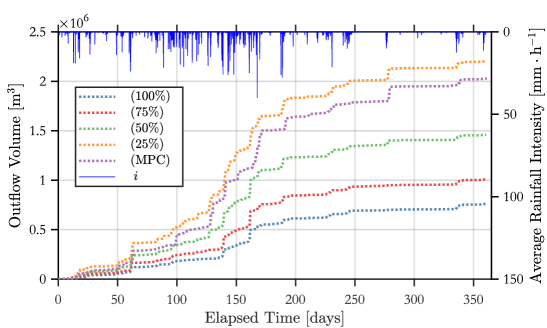
Figure 12: Treated volume for varied types of static controls and for the MPC control.

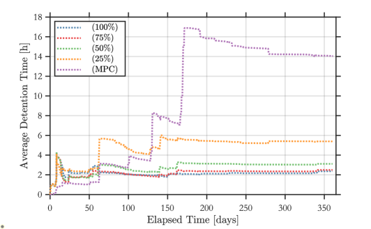
Figure 13: Average detention time curves for 1-yr of continuous simulation, where the MPC alternative aims to provide 18-hours of detention time.

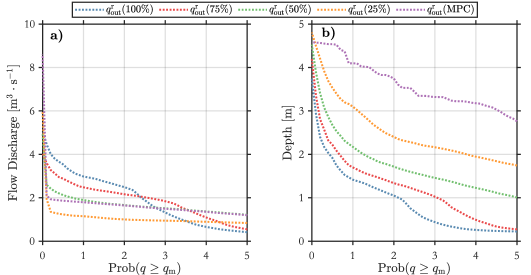
Figure 14: Duration curves for 1-yr of continuous simulation, where (a) is flow duration curve for scenarios of 100, 75, 50, and 25% in the valve openness, compared to the MPC controlled case Part (b) represents the stage duration curve.

4 Conclusions

A watershed-distributed continuous hydrodynamic model coupled with a reservoir model is integrated and a model predictive control algorithm is used to optimally control the valves and gates of a real-world reservoir. The reservoir control uses an objective changing condition according to predicted inflows. By switching the focus from flood mitigation to runoff detention, it was possible to achieve flood and proxy water quality control represented by specific minimum detention times. The general conclusions of this paper are described as follows:

• Reservoirs can be better controlled with larger orifice capacities since they can be adapted for relatively large flooding events and can have their hydraulic devices partially closed to allow flow mitigation under minor flooding events. By having a larger total orifice capacity, the reservoir can now better regulate flows and adapt to a wider variety of inflow hydrographs rather than a reservoir with a limited orifice capacity. Therefore, oversized reservoirs in terms of having relatively large orifice dimensions can be more flexible to deal with relatively larger or smaller events with active control. This conclusion is important since several reservoirs are in the path of the Aricanduva River and most of them are reportedly having poor mitigation effects for minor floods.

• More research is required to investigate the trade-offs among the MPC control variables of the prediction horizon, control horizon, and control steps. Although fixed and assumed in this paper, these parameters change the efficiency of the runoff control of reservoirs.

In addition to the general conclusions, each numerical case study had specific questions that were answered as

• A1 - The watershed quasi 2D kinematic wave hydrodynamic model was able to provide similar results when compared to the HEC-RAS 2D full momentum solver, with a better performance when using 10-m resolution than 30-m spatial resolution.

• A2 & A3 - During two consecutive 6-hour spanning 10-year storms, the MPC algorithm successfully controlled the valve and spillway of the detention pond, allowing not only a better flood mitigation performance, but also guaranteeing a desired detention pond to the stored volume when compared to the passive scenario with valve and spillway fully opened.

• A4 & A5 - The results of a 1-yr continuous simulation indicate that the MPC can regulate the flow discharges at the cost of generally maintaining a typical larger water level stored in the reservoir compared to passive scenarios. The MPC approach outperformed all passive scenarios in terms of flood mitigation and increasing detention times to a desired level.

The results presented in this paper show how a real-world detention pond can perform better in flood mitigation and water quality treatment by changing the operation of the reservoir from a passive gravity control approach to an active and real-time opening and closing of valves and gates. Sources of uncertainty, such as (i) rainfall forecasting, (ii) conceptual model simplifications, and (iii) lack of correcting states with techniques such as Kalman filters, are important aspects that could be incorporated into future studies.

Some important limitations must be addressed in future studies to understand the robustness of MPC applied to real-world stormwater reservoirs. First, the uncertainty in the rainfall predictions must be assessed to understand whether the MPC can still perform better than a passive scenario or not under these circumstances. In addition, the hydrological model itself has its own uncertainty in the conceptualization that can also underestimate the inflow hydrographs, leading to a not actually optimized control schedule of valves and gates. To this end, a self-controlled system is desired. The hydrological models used to simulate the watershed processes provide simple estimates of the system states that can be further corrected by real-time field measurements, autocorrecting, and auto-calibrating the model with a Kalman Filter approach. Investigating the aforementioned issues are future directions to improve understanding of how MPC applied to detention ponds can improve flood mitigation and water quality treatment.

In addition, the proposed control strategy in this paper can also be subjected to failures if extremely large storms are rapidly predicted. For example, in the case of a large hurricane or a rapid (i.e., within a prediction horizon) flash flood, and the reservoir was storing water for water quality purposes, the system might not be feasible to take up the event due to the limited available storage capacity. Therefore, the numerical approach presented here can also be used solely to investigate the effects of flood control or water quality control instead, or both combined.

To successfully adapt the approach presented here to other reservoirs, modelers have to tune the weights of the objective functions representing the trade-offs between control effort and flow mitigation, the thresholds for large and minor flood events, the expected detention time, and ultimately the expected maximum flow discharge released after reaching the water quality detention time. These are parameters that can be easily adapted to local regulations and estimated with hydrological data, allowing for an improvement in the performance of detention ponds for flood mitigation and runoff detention.

5 Data Availability Statement

Some or all data, models, or code generated or used during the study are available in a repository or online in accordance with funder data retention policies. All software can be freely downloaded in (Gomes Jr., 2024).

Supplemental Materials

Supplementary data related to this article can be found at https://github.com/marcusnobrega-eng/RTC---Flood-and-Water-Quality.

References

- Akan and Iyer (2021) Akan, A.O., Iyer, S.S., 2021. Open channel hydraulics. Butterworth-Heinemann.
- Bilodeau et al. (2018) Bilodeau, K., Pelletier, G., Duchesne, S., 2018. Real-time control of stormwater detention basins as an adaptation measure in mid-size cities. Urban Water Journal 15, 858–867.
- Brown et al. (2022) Brown, C.F., Brumby, S.P., Guzder-Williams, B., Birch, T., Hyde, S.B., Mazzariello, J., Czerwinski, W., Pasquarella, V.J., Haertel, R., Ilyushchenko, S., et al., 2022. Dynamic world, near real-time global 10 m land use land cover mapping. Scientific Data 9, 251.
- Brunner (2016) Brunner, G., 2016. Hec-ras river analysis system, 2d modeling user’s manual, version 5.0. Davis: US Army Corps of Engineers, hydrologic engineering center .
- Cook (2007) Cook, E.A., 2007. Green site design: Strategies for storm water management. Journal of Green Building 2, 46–56.
- Courant et al. (1928) Courant, R., Friedrichs, K., Lewy, H., 1928. Über die partiellen differenzengleichungen der mathematischen physik. Mathematische annalen 100, 32–74.
- Downer et al. (2006) Downer, C.W., Ogden, F.L., et al., 2006. Gridded surface subsurface hydrological analysis (gssha) user’s manual; version 1.43 for watershed modeling system 6.1 .
- French and French (1985) French, R.H., French, R.H., 1985. Open-channel hydraulics. McGraw-Hill New York.
- Gao et al. (2020) Gao, C., He, Z., Pan, S., Xuan, W., Xu, Y.P., 2020. Effects of climate change on peak runoff and flood levels in qu river basin, east china. Journal of Hydro-environment Research 28, 34–47.
- Gomes Jr. (2024) Gomes Jr., 2024. Stormwater-rtc (v12). https://github.com/marcusnobrega-eng/RTC---Flood-and-Water-Quality.
- Gomes Júnior et al. (2022) Gomes Júnior, M.N., Giacomoni, M.H., Taha, A.F., Mendiondo, E.M., 2022. Flood risk mitigation and valve control in stormwater systems: State-space modeling, control algorithms, and case studies. Journal of Water Resources Planning and Management 148, 04022067.
- Green and Ampt (1911) Green, W.H., Ampt, G.A., 1911. Studies on soil phyics. The Journal of Agricultural Science 4, 1–24.
- Greenlee (1987) Greenlee, D.D., 1987. Raster and vector processing for scanned linework. Photogrammetric Engineering and Remote Sensing 53, 1383–1387.
- de Hidráulica (2020) de Hidráulica, F.C.T., 2020. Caderno de bacia hidrográfica: bacia do córrego aricanduva. Prefeitura do Município de São Paulo - Secretaria Municipal de Infraestrutura Urbana e Obras , 272.
- Ibrahim (2020) Ibrahim, Y.A., 2020. Real-time control algorithm for enhancing operation of network of stormwater management facilities. Journal of Hydrologic Engineering 25, 04019065.
- Lu et al. (2022) Lu, M., Yu, Z., Hua, J., Kang, C., Lin, Z., 2022. Spatial dependence of floods shaped by extreme rainfall under the influence of urbanization. Science of The Total Environment , 159134.
- Maiolo et al. (2020) Maiolo, M., Palermo, S.A., Brusco, A.C., Pirouz, B., Turco, M., Vinci, A., Spezzano, G., Piro, P., 2020. On the use of a real-time control approach for urban stormwater management. Water 12, 2842.
- Miller and Hutchins (2017) Miller, J.D., Hutchins, M., 2017. The impacts of urbanisation and climate change on urban flooding and urban water quality: A review of the evidence concerning the united kingdom. Journal of Hydrology: Regional Studies 12, 345–362.
- Mullapudi et al. (2020) Mullapudi, A., Lewis, M.J., Gruden, C.L., Kerkez, B., 2020. Deep reinforcement learning for the real time control of stormwater systems. Advances in water resources 140, 103600.
- Naughton et al. (2021) Naughton, J., Sharior, S., Parolari, A., Strifling, D., McDonald, W., 2021. Barriers to real-time control of stormwater systems. Journal of Sustainable Water in the Built Environment 7, 04021016.
- Oh and Bartos (2023) Oh, J., Bartos, M., 2023. Model predictive control of stormwater basins coupled with real-time data assimilation enhances flood and pollution control under uncertainty. Water Research 235, 119825.
- PMSP (2017) PMSP, S.P.P.M.d.S.P., 2017. Portal geosampa. URL: http://geosampa.prefeitura.sp.gov.br/PaginasPublicas/_SBC.aspx#. accessed: 12-04-2022.
- Rossman (2010) Rossman, L.A., 2010. Storm water management model user’s manual, version 5.0. National Risk Management Research Laboratory, Office of Research and ….
- Rossman and Huber (2016) Rossman, L.A., Huber, W.C., 2016. Storm water management model reference manual. Volume III—Water Quality .
- Sadler et al. (2020) Sadler, J.M., Goodall, J.L., Behl, M., Bowes, B.D., Morsy, M.M., 2020. Exploring real-time control of stormwater systems for mitigating flood risk due to sea level rise. Journal of Hydrology 583, 124571.
- Schmitt et al. (2020) Schmitt, Z.K., Hodges, C.C., Dymond, R.L., 2020. Simulation and assessment of long-term stormwater basin performance under real-time control retrofits. Urban Water Journal 17, 467–480.
- Schwanghart and Scherler (2014) Schwanghart, W., Scherler, D., 2014. Topotoolbox 2–matlab-based software for topographic analysis and modeling in earth surface sciences. Earth Surface Dynamics 2, 1–7.
- Sentelhas et al. (2010) Sentelhas, P.C., Gillespie, T.J., Santos, E.A., 2010. Evaluation of fao penman–monteith and alternative methods for estimating reference evapotranspiration with missing data in southern ontario, canada. Agricultural water management 97, 635–644.
- Sharior et al. (2019) Sharior, S., McDonald, W., Parolari, A.J., 2019. Improved reliability of stormwater detention basin performance through water quality data-informed real-time control. Journal of Hydrology 573, 422–431.
- Smith (2024) Smith, A.B., 2024. 2023: A historic year of u.s. billion-dollar weather and climate disasters. URL: https://www.climate.gov/news-features/blogs/beyond-data/2023-historic-year-us-billion-dollar-weather-and-climate-disasters. accessed: 29-01-2024.
- Vosselman (2000) Vosselman, G., 2000. Slope based filtering of laser altimetry data. International archives of photogrammetry and remote sensing 33, 935–942.
- Walsh et al. (2001) Walsh, C.J., Sharpe, A.K., Breen, P.F., Sonneman, J.A., 2001. Effects of urbanization on streams of the melbourne region, victoria, australia. i. benthic macroinvertebrate communities. Freshwater Biology 46, 535–551.
- Webber et al. (2022) Webber, J.L., Fletcher, T., Farmani, R., Butler, D., Melville-Shreeve, P., 2022. Moving to a future of smart stormwater management: A review and framework for terminology, research, and future perspectives. Water Research , 118409.
- Winsemius et al. (2016) Winsemius, H.C., Aerts, J.C., Van Beek, L.P., Bierkens, M.F., Bouwman, A., Jongman, B., Kwadijk, J.C., Ligtvoet, W., Lucas, P.L., Van Vuuren, D.P., et al., 2016. Global drivers of future river flood risk. Nature Climate Change 6, 381–385.
- Wong and Kerkez (2018) Wong, B., Kerkez, B., 2018. Real-time control of urban headwater catchments through linear feedback: Performance, analysis, and site selection. Water Resources Research 54, 7309–7330.
- Zahmatkesh et al. (2015) Zahmatkesh, Z., Burian, S.J., Karamouz, M., Tavakol-Davani, H., Goharian, E., 2015. Low-impact development practices to mitigate climate change effects on urban stormwater runoff: Case study of new york city. Journal of Irrigation and Drainage Engineering 141, 04014043.
- Zhang et al. (2018) Zhang, P., Cai, Y., Wang, J., 2018. A simulation-based real-time control system for reducing urban runoff pollution through a stormwater storage tank. Journal of cleaner production 183, 641–652.