End-to-end Conditional Robust Optimization

Abstract

The field of Contextual Optimization (CO) integrates machine learning and optimization to solve decision making problems under uncertainty. Recently, a risk sensitive variant of CO, known as Conditional Robust Optimization (CRO), combines uncertainty quantification with robust optimization in order to promote safety and reliability in high stake applications. Exploiting modern differentiable optimization methods, we propose a novel end-to-end approach to train a CRO model in a way that accounts for both the empirical risk of the prescribed decisions and the quality of conditional coverage of the contextual uncertainty set that supports them. While guarantees of success for the latter objective are impossible to obtain from the point of view of conformal prediction theory, high quality conditional coverage is achieved empirically by ingeniously employing a logistic regression differentiable layer within the calculation of coverage quality in our training loss. We show that the proposed training algorithms produce decisions that outperform the traditional estimate then optimize approaches.

1 Introduction

In a standard Machine Learning (ML) setting, $\Psi\subseteq\mathbb{R}^{m}$ represent the input set and $\Xi\subseteq\mathbb{R}^{m}$ represent the output sets and we aim to learn a model ${\mathfrak{F}}_{\theta}$ parameterized by $\theta$ that approximates the relationship between the input and output sets. In real-world applications, we usually have a dataset of $M$ samples, ${\mathcal{D}_{\psi\xi}}:=\{(\psi_{i},\xi_{i})\}_{i=1}^{M}$ which are used to approximate the underlying input-output relationship learned by the model. For a new data sample $\psi\in\Psi$, the model trained on ${\mathcal{D}_{\psi\xi}}$ is used to predict a corresponding target $\xi={\mathfrak{F}}_{\theta}(\psi)$. Recently, there has been a growing interest in integrating this estimation process with the subsequent optimization process. In this context, the prediction is used within a cost minimization problem $\hat{x}^{*}(\psi):=\arg\mathop{\rm min}_{x\in\mathcal{X}}c(x,{\mathfrak{F}}_{\theta}(\psi))$, where $\mathcal{X}\subseteq\mathbb{R}^{n}$ is the set of feasible decisions and $c(x,\xi)$ the cost function. The intent is to produce an adapted decision with low out-of-sample expected cost ${\mathbb{E}}[c(\hat{x}^{*}(\psi),\xi)]$. When there a mismatch between the predictive loss $\mathcal{L}$ and the cost function $c(x,\xi)$, a small error in estimating $\xi$ for a given $\psi$ can lead to highly suboptimal $x^{*}(\psi)$ (see Elmachtoub and Grigas [2022]). Task-based (or decision-focused) learning (c.f. Mandi et al. [2023], Donti et al. [2017]) addresses this issue by training the model ${\mathfrak{F}}_{\theta}$ directly on the performance of the policy $x^{*}(\psi)$. By trading off predictive performance in favour of task performance, the task-based approach can give near optimal decisions.

In high stakes applications, a DM usually demonstrates of a certain degree of risk aversion by requiring some level of protection against a range of plausible future scenarios. A natural risk averse variant of integrated ML and optimization takes the form of Conditional Robust Optimization (see Chenreddy et al. [2022]), which integrates conformal prediction with robust optimization. Specifically, machine learning is first used to produce a contextually adapted uncertainty set ${\mathcal{U}}(\psi)$ known to contain with high probability the realized $\xi$, which is then inserted to the conditional robust optimization model:

$$x^{*}(\psi):=\arg\mathop{\rm min}_{x\in\mathcal{X}}\mathop{\rm max}_{\xi\in\mathcal{U}(\psi)}c(x,\xi),$$ (1)

To this date, the methods proposed in the literature follow an Estimate Then Optimize (ETO) paradigm. Namely, data is first used to calibrate the contextual uncertainty set. This set is then used as an input to the CRO problem to get the adapted robust decision $x^{*}(\psi)$. However, this uncertainty set calibration process does not consider the downstream optimization task which can lead to misalignment between the initial estimation loss function and the robust optimization objectives.

In this paper, we propose a novel end-to-end learning framework for conditional robust optimization that constructs the contextual uncertainty set by accounting for the downstream task loss. Our contributions can be described as follows:

• We propose for the first time an end-to-end training algorithm to produce contextual uncertainty sets that lead to reduced risk exposure for the solution of the down-stream CRO problem.

• We introduce a novel joint loss function aimed at enhancing the conditional coverage of the contextual uncertainty sets $\mathcal{U}(\psi)$ while improving the CRO objective

• We demonstrate through a set of synthetic environments that our end-to-end approach surpasses ETO approaches at the CRO task while achieving comparable if not superior conditional coverage with its learned contextual set.

• We show empirically how our end-to-end learning approach outperforms other state-of-the-art methods on a portfolio optimization problem using the real world data from the US stock market.

2 Related work

Estimate Then Optimize Popularized by the initial work of Hannah et al. [2010] is a framework that integrates ML and optimization tasks. Several approaches are proposed to learn the conditional distribution from data. Kannan et al. [2023], Sen and Deng [2018] propose using residuals from the trained regression model to learn conditional distributions. Bertsimas and Kallus [2020] approach assigns weights to the historical observations of the parameters and solves the weighted SAA problem. Besides the CSO problems, There has been a growing interest in integrating ML techniques in Robust Optimization problems.Chenreddy et al. [2022] identifies clusters of the uncertain parameters based on the covariate data and calibrates the sets for these clusters. Patel et al. [2023] propose using non-convex prediction regions to construct uncertainty sets.Blanquero et al. [2023] constructs contextual ellipsoidal uncertainty sets by making normality assumptions. Ohmori [2021] uses non-parametric kNN model to identify the minimum volume ellipsoid to be used as an uncertainty set. Sun et al. [2024] solves a robust contextual LP problem where a prediction model is first learned, then uncertainty is calibrated to match robust objectives. It is to be noted that all these CRO approaches follow the ETO paradigm.

End-to-end learning is a more recent stream of work that integrates the Estimation and Optimization tasks and trains using the downstream loss. Donti et al. [2017] proposed using an end-to-end approach for learning probabilistic machine learning models using task loss. Elmachtoub and Grigas [2022] learns contextual point predictor by minimizing the regret associated with implementing prescribed action based on the mean estimator. Amos and Kolter [2017] uses implicit differentiation methods to train an end-to-end model. Butler and Kwon [2023] solves large-scale QPs using the ADMM algorithm that decouples the differentiation procedure for primal and dual variables. Elmachtoub and Grigas [2022], Mandi et al. [2020] propose using a surrogate loss function to train integrated methods to address loss functions with non-informative gradients. Wang et al. [2023] proposes learning a non-contextual uncertainty set by maximizing the expected performance across a set of randomly drawn parameterized robust constrained problems while ensuring guarantees on the probability of constraint satisfaction with respect to the joint distribution over perturbance and robust problems. Costa and Iyengar [2023] proposes a distributionally robust end-to-end system that integrates point prediction and robustness tuning to the portfolio construction problem. We refer the reader to Sadana et al. [2023] for a broader discussion on both ETO and end-to-end models.
Uncertainty quantification methods are employed to estimate the confidence of deep neural networks over their predictions Kontolati et al. [2022]. Common UQ approaches include using Bayesian methods like stochastic deep neural networks, ensembling over predictions from several models to suggest intervals and models that directly predict uncertain intervals. Gawlikowski et al. [2021]. Beyond estimating predictive uncertainty, ensuring its statistical reliability is crucial for safe decision-making Guo et al. [2017]. Conformal prediction has become popular as a distribution-free calibration method Shafer and Vovk [2008]. Although conformal prediction ensures marginal coverage, attaining conditional coverage in the most general case is desirable Vovk [2012]. Although considered unfeasible Romano et al. [2020] offers group conditional guarantees for disjoint groups by independently calibrating each group.

3 Estimate then Robust Optimize

The concept of “estimate then optimize”(ETO) comes from the contextual optimization literature (see Sadana et al. [2023]). In this framework, the role of the Estimation process is to quantify the uncertainty about $\xi$ given the observed $\psi$. This is given as input to an Optimization problem that prescribes an optimal contextual decision $x^{*}(\psi)$.

When the downstream optimization problem is a CRO problem, the estimation step is required to produce a region that adapts to the observed covariates $\psi$ and is expected to contain the response $\xi$ with high confidence. This can be done indirectly by first calibrating a conditional distribution model $F_{\theta}(\psi)$ to the data, followed by an implied confidence region ${\mathcal{U}}_{\theta}(\psi)$ that satisfies ${\mathbb{P}}_{F_{\theta}(\psi)}(\xi\in{\mathcal{U}}_{\theta}(\psi))=1-\epsilon$. For e.g., when one assumes that $\xi|\psi\sim\mathcal{N}(\hat{\mu}(\psi),\hat{\Sigma}(\psi))$, one can learn $(\hat{\mu}(\psi),\hat{\Sigma}(\psi))$ by maximizing the log-likelihood function (see Barratt and Boyd [2023])

$$-\frac{n}{2}\log(2\pi)+\sum_{j=1}^{n}\log L(\psi)_{jj}-\frac{1}{2}\|L(\psi)^{\top}(\xi-\hat{\nu}(\psi))\|_{2}^{2}$$

where $L(\psi)$ and $\hat{\nu}(\psi)$ are the parametric mappings that can be used to compose $\hat{\mu}(\psi):=L(\psi)^{\top}\nu(\psi)$ and $\hat{\Sigma}(\psi)=L(\psi)^{-\top}L(\psi)^{-1}$. Using the $\alpha$ quantile from the chi-squared distribution with $m$ degrees of freedom, one can define ${\mathcal{U}}_{\theta}(\psi)$ that satisfies ${\mathbb{P}}(\xi\in{\mathcal{U}}_{\theta}(\psi))=1-\epsilon$ asymptotically.

Some recent work completely circumvents the need for the $F_{\theta}$ intermediary by calibrating some ${\mathcal{U}}_{\theta}(\psi)$ directly on the dataset. For e.g. Chenreddy et al. [2022] propose identifying a k-class classifier, $a:\mathbb{R}^{m}\rightarrow[K]$ to reduce $\mathcal{U}_{\theta}(\psi):=\mathcal{U}_{\theta}(a(\psi))$ such that ${\mathbb{P}}(\xi\in{\mathcal{U}}_{\theta}(k)|a(\psi)=k)\geq 1-\epsilon\,\forall k$. The literature on conformal prediction belongs to the second type and separates the calibration of the shape of ${\mathcal{U}}(\psi)$ from the calibration of its size, parametrized by a radius $r>0$, on a reserved validation set in order to provide out-of-sample marginal coverage guarantees of the form ${\mathbb{P}}(\xi\in{\mathcal{U}}(\psi))\geq 1-\epsilon,$ where the probability is taking over both the draw of the validation set and of the next sample.

4 End-to-End Conditional Robust Optimization

While the ETO approach presented in the section 3 presents an efficient way to conditionally quantify the uncertainty, it does not take into account the quality of the decisions $x^{*}(\psi)$ that is prescribed by the downstream CRO model. In practice, the quality of a robust decision is usually assessed by measuring the risks associated to the cost produced on a new data sample (a.k.a. out-of-sample). We assume that this risk is measured by a risk measure that reflect the amount of risk aversion experienced by the DM. For instance, one can use conditional value-at-risk with $\rho_{\alpha}(X):=\mathop{\rm inf}_{t}t+(1/(1-\alpha))E[(X-t)^{+}]$, which computes the expected value in the right tail of the random cost and covers both expected value and the worst-case cost as special cases (i.e. with $\alpha=0$ and $1$ respectively). Motivated by recent evidence (see Elmachtoub and Grigas [2022]) indicating that performance improvement can be achieved by employing a decision-focused/task-based learning paradigm, we propose end-to-end conditional robust optimization.

4.1 The ECRO training problem

Formally, we let $\Psi\subseteq\mathbb{R}^{m}$ be an arbitrary support set for $\psi$ whereas $\Xi\subseteq\mathbb{R}^{m}$ is assumed for simplicity to be contained within a ball centered at 0 of radius $R_{\xi}$. We consider $c(x,\xi)$ to be convex in $x$ and concave in $\xi$ and let $\mathcal{X}(\psi):=\{x\in\mathbb{R}^{n}|g(x,\psi)\leq 0,\,h(x,\psi)=0\}$ be a convex feasible set for $x$, possibly dependent on $\psi$, and defined through a set of convex inequalities, identified using $g:\mathbb{R}^{n}\times\mathbb{R}^{m}\rightarrow\mathbb{R}^{J}$ and affine equalities, identified using an affine mapping $h:\mathbb{R}^{n}\times\mathbb{R}^{m}\rightarrow\mathbb{R}^{J}$. The conditional optimal policy then becomes:

$$x^{*}(\psi,{\mathcal{U}}):=\arg\mathop{\rm min}_{x\in\mathcal{X}(\psi)}\mathop{\rm max}_{\xi\in\mathcal{U}(\psi)}c(x,\xi),$$ (2)

where we make explicit how the decision depends on both the contextual uncertainty set and the realized covariate. Given a parametric family of contextual uncertainty set ${\mathcal{U}}_{\theta}$ with $\theta\in\Theta$ and a dataset $D_{\psi\xi}:=\{(\psi^{i},\xi^{i})\}_{i=1}^{M}$, the ECRO training problem consists in identifying

$$\mathop{\rm min}_{\theta\in\Theta}\mathcal{L}_{ECRO}(\theta):=\rho_{i\sim M}(c(x^{*}(\psi^{i},\mathcal{U}_{\theta}),\xi^{i})),$$ (3)

where for simplicity we assume $\rho(\cdot)$ to be a conditional value-at-risk measure, and ${\mathcal{U}}_{\theta}(\psi)$ to be ellipsoidal for all $\psi$. Namely, we can assume that

$$\mathcal{U}_{\theta}(\psi)=\mathcal{E}(\mu_{\theta}(\psi),\Sigma_{\theta}(\psi),r)$$ (4)

$$\;:=\{\ \xi\in\mathbb{R}^{{m}}:(\xi-\mu_{\theta}(\psi))^{T}\Sigma_{\theta}(\psi)^{-1}(\xi-\mu_{\theta}(\psi))\leq 1\}\,,$$

for some $\mu_{\theta}:\mathbb{R}^{m}\rightarrow\mathbb{R}^{m}$ and $\Sigma_{\theta}:\mathbb{R}^{m}\rightarrow\mathcal{S}_{+}$, where $\mathcal{S}_{+}$ is the set of positive definite matrices, for all $\theta\in\Theta$. While the robust optimization literature suggests various uncertainty set structures that facilitates resolution of the RO problem, the ellipsoidal set stands out as a natural one to employ as it retains numerical tractability (see Ben-Tal and Nemirovski [1998]) and can easily be described to the DM.

Figure 1: Training pipeline for task-based learning

The training pipeline for the tasked-based learning approach is illustrated in figure 1. In this pipeline, one starts from an arbitrary $\theta^{0}$, the optimization problem (2) is solved first for each data point, the resulting optimal actions are then implemented in order to measure the empirical risk under $D_{\psi\xi}$, which we call empirical ECRO loss of $\theta^{0}$. A gradient of $\mathcal{L}_{ECRO}(\theta)$ can then be used to update $\theta^{0}$ in a direction of improvement. Key steps in in this pipeline consists in computing $x^{*}(\psi^{i},{\mathcal{U}}_{\theta})$ efficiently and in a way that enables differentiation with respect to $\theta$.

4.2 Reducing and solving the robust optimization task

Given the convex-concave structure of $c(x,\xi)$ and the convexity and compactness of the ellipsoidal set, we can employ Fenchal duality (see Ben-Tal et al. [2015]) to reformulate the min-max problem as a simpler minimization form over an augmented decision space. Specifically, we first replace the original cost function with the equivalent cost

$$\bar{c}(x,\xi):=\left\{\begin{array}[]{cl}c(x,\xi)&\mbox{if $\|\xi\|_{2}\leq R$}\\ -\infty&\mbox{otherwise}\end{array}\right.,$$

which integrates information about the domain of $\xi$. One can then employ theorem 6.2 of Ben-Tal et al. [2015], to show that problem (1) can be reformulated as:

$$\mathop{\rm min}_{x\in\mathcal{X}(\psi),v}f(x,v,\psi):=\delta^{*}(v|\mathcal{U}_{\theta}(\psi))-\bar{c}_{*}(x,v)$$ (5)

where the support function

$$\delta^{*}(v|\mathcal{U}_{\theta}(\psi)):=\mathop{\rm sup}_{\xi\in\mathcal{U}_{\theta}(\psi)}\xi^{T}v=\mu^{T}v+\sqrt{v^{T}\Sigma^{-1}v}$$ (6)

while the partial concave conjugate function is defined as

$$\bar{c}_{*}(x,v):=\mathop{\rm inf}_{\xi}v^{T}\xi-\bar{c}(x,\xi)=\mathop{\rm inf}_{\xi:\|\xi\|_{2}\leq R}v^{T}\xi-c(x,\xi)$$

This leads to $x^{*}(\psi,\mathcal{U}(\psi))$ being the minimizer of the convex minimization problem:

$$\mathop{\rm min}_{x\in\mathcal{X}(\psi),v}f(x,v,\psi)$$ (7)

with $f(x,v,\psi):=\mu^{T}v+\sqrt{v^{T}\Sigma^{-1}v}-\bar{c}_{*}(x,v)$, a jointly convex function of $x$ and $v$ and finite valued over its domain, and with sub-derivatives:

$$\nabla_{x}f(x,v,\psi)=\mu+(1/\sqrt{v^{T}\Sigma^{-1}v})v-\xi^{*}(x,v)$$

$$\nabla_{v}f(x,v,\psi)=\nabla_{x}c(x,\xi^{*}(x,v)),$$

where $\xi^{*}(x,v):=\mathop{\rm argmin}_{\xi:\|\xi\|_{2}\leq R}v^{T}\xi-c(x,\xi)$. Revisiting the procedure outlined in Figure 1, one can observe that the training process requires a forward pass to find the optimal solutions and a backward pass to iteratively update the parameter vector $\theta$. This requires the computation of the gradients of the solution to the problem 3 with respect to the input parameters which are passed through the reformulated CRO problem. Furthermore, the minimization procedure in problem 3 entails navigating through the risk measure $\rho$. These aspects will be further explored in the next section.

4.3 Gradient for problem (3)

In training problem (3), the gradient of $\mathcal{L}_{ECRO}(\theta)$ with respect to $\theta$ can be obtained using the chain rule:

$$\allowdisplaybreaks\nabla_{\theta} \mathcal{L}_{ECRO}(\theta)=\sum_{i}\frac{\partial\rho_{i\sim M}(y_{i})}{\partial y_{i}}\big{|}_{y_{i}=c(x^{*}(\psi^{i},\mathcal{U}_{\theta}),\xi^{i})}\cdot\nabla_{{{\bm{x}}}}c({{\bm{x}}})\big{|}_{{{\bm{x}}}=x^{*}(\psi^{i},\mathcal{U}_{\theta})}\cdot$$

$$\quad\left(\nabla_{\mu}x^{*}(\psi^{i},\mathcal{E}(\mu,\Sigma_{\theta}(\psi^{i})))\big{|}_{\mu=\mu_{\theta}(\psi^{i})}\nabla_{\theta}\mu_{\theta}(\psi^{i})\right.\left.+\nabla_{\Sigma}x^{*}(\psi^{i},\mathcal{E}(\mu_{\theta}(\psi^{i}),\Sigma))\big{|}_{\Sigma=\Sigma_{\theta}(\psi^{i})}\nabla_{\theta}\Sigma_{\theta}(\psi^{i})\right).$$

Based on Ruszczyński and Shapiro , when $\rho(Y):=\mbox{CVaR}_{\alpha}(Y)$, one can employ the subdifferential:

$$\nabla_{{{\bm{y}}}}\rho_{i\sim M}(y_{i}):={{\bm{\upsilon}}}({{\bm{y}}})$$

with ${{\bm{\upsilon}}}({{\bm{y}}})\in\mathop{\rm argmax}_{{{\bm{\upsilon}}}\in\mathbb{R}^{M}_{+}:{{\bm{1}}}^{T}{{\bm{\upsilon}}}=1,{{\bm{\upsilon}}}\leq((1-\alpha)N)^{-1}}{{\bm{\upsilon}}}^{T}{{\bm{y}}}$.

Given that $\nabla_{{{\bm{x}}}}c({{\bm{x}}})$, $\nabla_{\theta}\mu_{\theta}(\psi)$, and $\nabla_{\theta}\Sigma_{\theta}(\psi)$ can be readily obtained using Auto-Differentiation Seeger et al. [2017] when $c({{\bm{x}}})$, $\mu_{\theta}(\psi)$, and $\Sigma_{\theta}(\psi)$ are differentiable, we focus the rest of this subsection on the process of identifying $\nabla_{(\mu,\Sigma)}x^{*}(\psi,\mathcal{E}(\mu,\Sigma))$. Following the decision-focus learning literature (see Blondel et al. [2022]), one can identify such derivatives by exploiting the fact that any optimal primal dual pair $(x^{*},v^{*},\lambda^{*},\nu^{*})$ of problem (7) must satisfy the Karush-Kuhn-Tucker (KKT) conditions, which take the form:

$$G(x^{*},v^{*},\lambda^{*},\nu^{*},\mu,\Sigma,\psi)=0,\qquad g(x^{*},\psi)\leq 0,\lambda^{*}\geq 0.$$

where

$$G(x^{*},v^{*},\lambda^{*},\nu^{*},\mu,\Sigma,\psi):=\begin{bmatrix}\nabla_{x}f(x^{*},v^{*},\psi)+\nabla_{x}g(x^{*},\psi)^{T}\lambda^{*}+\nabla_{x}h(x^{*},\psi)^{T}\nu^{*}\\ \lambda^{*}\circ g(x^{*},\psi)\\ h(x^{*},\psi)\end{bmatrix}$$

and $\circ$ denotes the Hadamard product of two vectors.

One can therefore apply implicit differentiation to the constraints $G(x^{*},v^{*},\lambda^{*},\nu^{*},\mu,\Sigma,\psi)=0$ to identify $\nabla_{(\mu,\Sigma)}x^{*}(\psi,\mathcal{E}(\mu,\Sigma))$ simultaneously with the derivatives of $v^{*}$, $\lambda^{*}$, and $\nu^{*}$ with respect to the pair $(\mu,\Sigma)$. Specifically, one is required to solve the system of equations:

$$\frac{\partial}{\partial x,v,\lambda,\nu}G(x^{*},v^{*},\lambda^{*},\nu^{*},\mu,\Sigma,\psi)\cdot\frac{\partial}{\partial(\mu,\Sigma)}(x^{*},v^{*},\lambda^{*},\nu^{*})(\mu,\Sigma)=-\frac{\partial}{\partial(\mu,\Sigma)}G(x^{*},v^{*},\lambda^{*},\nu^{*},\mu,\Sigma,\psi),$$

where $\frac{\partial}{\partial(x,v,\lambda,\nu)}G$ denotes the Jacobian of the mapping $G$ with respect to $(x,v,\lambda,\nu)$. We refer to Blondel et al. [2022] and Duvenaud et al. [2020] for further details on the computations of related to implicit differentiation.

4.4 Task-based Set (TbS) Algorithm

In this section, we delve into implementation details of the ECRO training pipeline. Regarding the contextual ellipsoidal set $\mathcal{E}(\mu_{\theta}(\psi),\Sigma_{\theta}(\psi))$, we follow the ideas proposed in Barratt and Boyd [2023] and employ a neural network that maps from ${\mathfrak{F}}_{\theta}:\mathbb{R}^{m}\rightarrow\mathbb{R}^{m}\times\mathbb{R}^{m(m+1)/2}\times\mathbb{R}$. The first set of outputs is used to define $\mu_{\theta}(\psi)$ while the second and third set forms a lower triangular matrix $L_{\theta}(\psi)$ and scalar $r_{\theta}(\psi)$, which is made independent of $\psi$ w.l.o.g., used to produce $\Sigma_{\theta}(\psi):=r_{\theta}(\psi)L_{\theta}(\psi)L_{\theta}(\psi)^{T}$. The positive definiteness of $\Sigma_{\theta}(\psi)$ is ensured by taking an exponential in the last layer of the network for the output that appear in the diagonal of $L$. The architecture of the neural network can be found in appendix B.4.

The second set of notable details have to do with solving for $x^{*}(\psi^{i},\mathcal{E}(\mu^{i}_{\theta},\Sigma^{i}_{\theta},r_{\theta}))\ \forall i$. In our implementation of end-to-end learning for conditional robust optimization, we found that a trust region optimization (TRO) method Byrd et al. [2000] could efficiently solve the reformulated robust optimization problem (7) and provide primal dual solution pairs for this problem. Given that each episode of the training would pass through the same set of data points, we further observed that the training accelerated significantly (see figure in Appendix B.1) when the trust region was interrupted early (after $K=5$ iterations) as long as it would be warm started at the solution found at the previous epochs. Algorithm 1 presents our proposed training framework for the ECRO approach.

Algorithm 1 ECRO Training with Trust Region Solver

[1] input: dataset ${\mathcal{D}_{\psi\xi}}$, max epochs $T$, max TRO steps $K$, batch size $N$, protection level $\alpha$ Initialize a warm start buffer $\{\bar{x}_{1},\dots,\bar{x}_{M}\}$ with each $\bar{x}^{i}\in\mathcal{X}(\psi_{i})$ Initialize network parameters $\theta$ and $t=1$ not converged and ($t\leq T$) Sample a batch of $N$ indices $\mathcal{B}\subset\{1,\dots,M\}$ $i\in\mathcal{B}$ //Run TRO for up to $K$ steps $x_{i}^{t},\lambda_{i}^{t},\nu_{i}^{t}\leftarrow$ TRO($\bar{x}_{i}$, $\mu_{\theta}(\psi_{i}),\Sigma_{\theta}(\psi_{i}),K)$ $\bar{x}_{i}\leftarrow x_{i}^{t}$ Update warm start

compute $\mathcal{L}_{ECRO}(\theta)$ and $\nabla_{\theta}\mathcal{L}_{ECRO}(\theta)$ for $i\sim\mathcal{B}$ $\theta\leftarrow\theta-\mbox{step size}\cdot\nabla_{\theta}\mathcal{L}_{ECRO}(\theta)$

return $\theta$

5 End-to-End CRO with Conditional Coverage

Recall that the ETO framework summarized in section 3 focused on producing contextual uncertainty set with appropriate marginal coverage (of $1-\epsilon$) of the realization of $\xi$. The training pipeline in section 4 was at the other end of the spectrum, disregarding entirely the objective of coverage to increase task performance. In practice, coverage can be a heavy price to pay to obtain performance as it implies a loss in the explainability of the prescribed robust decision. It is becoming apparent that many DM suffer from algorithm aversion (see [Burton et al., 2020]) and could be reluctant to implementing a robust decision produced from an ill covering uncertainty set.

We further argue that traditional ETO might already face resistance to adoption given the type of coverage property attributed to the ETO sets, i.e. ${\mathbb{P}}(\xi\in{\mathcal{U}}(\psi))=1-\epsilon$. Indeed, marginal coverage guarantees only hold in terms of the joint sampling of $\psi$ and $\xi$. This implies that it offers no guarantees regarding the coverage of $\xi$ given the observed $\psi$ for which the decision is made. In fact, a 90% marginal coverage can trivially be achieved using $\Xi$ when $\psi\in\Psi$ and $\emptyset$ otherwise, as long as ${\mathbb{P}}(\psi\in\Psi)=1-\epsilon$. This is clearly an issue for applications with critical safety considerations and motivates seeking conditional coverage in addition to the marginal coverage when designing $\mathcal{U}(\psi)$. In this section, we outline a training procedure that integrates a sub-procedure that enhances the conditional coverage performance.

5.1 The conditional coverage training problem

We start by briefly formalizing the difference between the two types of coverage in the definition below.

Definition 5.1.

Given a confidence level $1-\epsilon$, a contextual uncertainty set mapping $\mathcal{U}(\cdot)$ is said to satisfy marginal coverage if ${\mathbb{P}}(\xi\in\mathcal{U}(\psi))=1-\epsilon$, and to satisfy conditional coverage if ${\mathbb{P}}(\xi\in\mathcal{U}(\psi)|\psi)=1-\epsilon$ almost surely.

The following lemma identifies a necessary and sufficient condition for a contextual set to satisfy conditional coverage.

Lemma 5.2.

A contextual uncertainty set ${\mathcal{U}}(\psi)$ satisfies conditional coverage, at confidence $1-\epsilon$, if and only if

$$\mathcal{L}_{\mbox{\scriptsize CC}}(\theta):={\mathbb{E}}[\,\left({\mathbb{P}}(\xi\in{\mathcal{U}}(\psi)|\psi)-(1-\epsilon)\right)^{2}\,]=0$$

Proof.

For any random variable $X$, one can show that :

$$X =1-\epsilon\mbox{ a.s}$$

$$\;\Rightarrow\;{\mathbb{E}}[(X-(1-\epsilon))^{2}]=1\cdot(1-\epsilon-(1-\epsilon))^{2}=0$$

and that, since $y^{2}\leq 0\Leftrightarrow y=0$,

$${\mathbb{E}} [(X-(1-\epsilon))^{2}]=0$$

$$\;\Rightarrow\;(X-(1-\epsilon))^{2}=0\mbox{ a.s.}\;\Rightarrow\;X=1-\epsilon\mbox{ a.s.}.$$

By letting $X:={\mathbb{P}}(\xi\in{\mathcal{U}}_{\theta}(\psi)|\psi)$, we obtain our result. ∎

Equipped with Lemma 5.2, we formulate the “theoretical” conditional coverage training problem as $\mathop{\rm min}_{\theta\in\Theta}\;\;\mathcal{L}_{CC}(\theta)$. Since the true conditional distribution ${\mathbb{P}}(\xi\in{\mathcal{U}}_{\theta}(\psi)|\psi)$ is typically inaccessible to the DM, we propose an approximation that will make $\mathcal{L}_{CC}(\theta)$ practical.

5.2 Regression-based Conditional Coverage Loss

Given a set ${\mathcal{U}}$, one can define a binary random variable $y(\psi,\xi,{\mathcal{U}}):={{\bm{1}}}\{\xi\in{\mathcal{U}}(\psi)\}$, and rewrite the conditional probability distribution ${\mathbb{P}}(\xi\in{\mathcal{U}}(\psi)|\psi)$ as ${\mathbb{P}}(y(\psi,\xi,{\mathcal{U}})=1|\psi)$. Using the i.i.d sample data in ${\mathcal{D}_{\psi\xi}}$, one can approximate this conditional probability using a parametric model, i.e. ${\mathbb{P}}(y(\psi,\xi,{\mathcal{U}})|\psi)\approx g_{\phi}(\psi)$ for some $\phi\in\Phi$. The parameters $\phi$ can be calibrated by minimizing the negative conditional log-likelihood of $\{y(\psi^{i},\xi^{i},{\mathcal{U}})\}_{i=1}^{M}$:

$$\phi^{*}({\mathcal{U}}):=\arg\mathop{\rm min}_{\phi\in\Phi}-\frac{1}{M}\sum_{i=1}^{M}\log g_{\phi}(\psi^{i})^{y^{i}}(1-g_{\phi}(\psi^{i}))^{1-y^{i}},$$ (8)

where $y_{i}:=y(\psi^{i},\xi^{i},{\mathcal{U}})$. Using the parametric approximation $g_{\phi^{*}({\mathcal{U}})}(\psi)\approx{\mathbb{P}}(\xi\in{\mathcal{U}}(\psi)|\psi)$ and replacing the unknown true distribution of $(\psi,\xi)$ with the empirical one, we obtain our regression-based conditional coverage loss function

$$\hat{\mathcal{L}}_{CC}(\theta):=\mathbb{E}^{\mathcal{{\mathcal{D}_{\psi\xi}}}}[(g_{\phi^{*}({\mathcal{U}}_{\theta})}(\psi)-(1-\epsilon))^{2}].$$

The gradient of $\hat{\mathcal{L}}_{CC}(\theta)$ can be obtained using similar decision-focused training methods as employed for $\mathcal{L}_{ECRO}(\theta)$ given that:

$$\nabla_{\theta} \hat{\mathcal{L}}_{CC}=\sum_{i=1}^{M}2(g_{\phi^{*}({\mathcal{U}}_{\theta})}(\psi^{i})-(1-\epsilon))\nabla_{\phi}g_{\phi^{*}({\mathcal{U}}_{\theta})}(\psi^{i})\cdot\sum_{j=1}^{M}\partial\phi^{*}(\mathcal{E}(\mu,\Sigma_{\theta}(\psi^{i})))/\partial y^{j}\cdot$$

$$\left(\nabla_{\mu}y^{j}(\psi^{j},\xi^{j},\mathcal{E}(\mu,\Sigma_{\theta}(\psi^{j})))\big{|}_{\mu=\mu_{\theta}(\psi^{j})}\nabla_{\theta}\mu_{\theta}(\psi^{j})\right.\left.+\nabla_{\Sigma}y^{j}(\psi^{j},\xi^{j},\mathcal{E}(\mu_{\theta}(\psi^{j}),\Sigma))\big{|}_{\Sigma=\Sigma_{\theta}(\psi^{j})}\nabla_{\theta}\Sigma_{\theta}(\psi^{j})\right),$$

where the main challenges reside again in the step of differentiating through the minimizer of problem (8).

5.3 Dual Task based Set (DTbS) algorithm

Figure 2: Training pipeline for dual task based learning

We conclude this section with the presentation of our novel integrated algorithm that learns the contextual uncertainty set network ${\mathfrak{F}}_{\theta}$ by incorporating both the risk mitigation and conditional coverage tasks in the training. Indeed our DTbS training algorithm minimizes the following double task loss function that trades off between the two task objectives:

$$\mathcal{L}_{DT}(\theta)=\gamma\mathcal{L}_{ECRO}(\theta)+(1-\gamma)\hat{\mathcal{L}}_{CC}(\theta)$$ (9)

The training pipeline for this algorithm can be seen in figure 2. It closely mirrors the structure of the TbS algorithm, with additional crucial steps to compute the necessary components of the loss presented in 9. Within each epoch, the predicted uncertainty set ${\mathcal{U}}_{\theta}$ serves two purposes: i) Optimizing CRO to find the optimal policy $x^{*}(\cdot,{\mathcal{U}}_{\theta})$ and assessing its associated risk; and ii) producing the binary variable $y(\psi,\xi,{\mathcal{U}}_{\theta})$, which regression leading to $g_{\phi^{*}({\mathcal{U}}_{\theta})}(\cdot)$ serves to quantify the quality of the conditional coverage. The sum of task losses produce $\mathcal{L}_{DT}(\theta)$, which can be differentiated using decision-focused learning methods. The regression model $g_{\phi}(\psi)$ take the form of a feed-forward neural network with a sigmoid activation in the final layer and optimized using stochastic gradient descent. Algorithm 2 in appendix A presents the details of this DTbS algorithm.

Remark 5.3.

It is to be noted that achieving distribution-free finite sample conditional coverage guarantees is known to be impossible in the conformal prediction literature (see Barber et al. [2020]). Recently, some progress has been made towards partial forms of conditional coverage guarantees (see Gibbs et al. [2023]) yet it is unclear what are the implications of exploiting such partial coverage properties for the downstream CRO decisions. It is also unclear how such conditional conformal prediction procedures could be integrated within and end-to-end CRO approach.

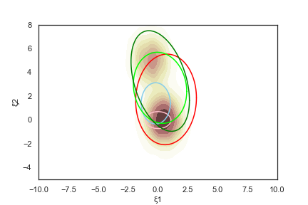
(a)

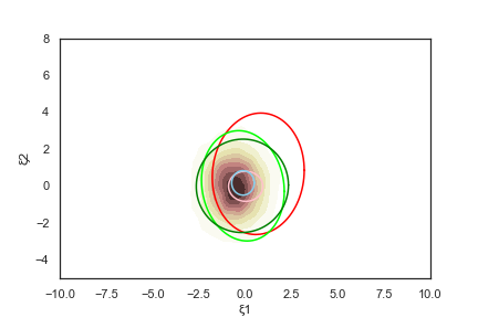
(b)

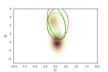
(c)

Figure 3: Comparison of uncertainty set ($\alpha$ = 0.9) coverage for different $\psi$ realizations: (a) $[2.5,-0.2]^{T}$, (b) $[-2.6,0.5]^{T}$, (c) $[2.7,1.9]^{T}$. The shade indicate the true conditional distribution.

   ETO-CPS     ETO-ACPS     ETO-DbS     TbS     DTbS

6 Experiments

This section outlines our experimental framework devised to demonstrate the advantages of the ECRO method in learning the uncertainty sets tailored to covariate information. Our focus lies in assessing the utility of the model in: i) improving the CRO performance; and ii) achieving conditional coverage. We conduct a comparative analysis between our two end-to-end approaches, TbS and DTbS, and three state-of-the-art ETO approaches to formulate contextual ellipsoidal sets. We first consider a Distribution-based contextual ellipsoidal uncertainty Set (ETO-DbS) recently introduced in Blanquero et al. [2023], where the conditional distribution of $\xi$ given $\psi$ is presumed to follow a multivariate normal distribution. Additionally, we explore two distributional-free approaches. A vanilla Conformal Prediction Set (ETO-CPS) uses conformal prediction on the output of a point predictor for $\xi$ given $\psi$, after shaping the ellipsoid (through an invariant $\Sigma$) using the residual errors Johnstone and Cox [2021]. An Adapted version of Conformal Prediction Set (ETO-ACPS) (proposed in Messoudi et al. [2022]) adapts the shape $\Sigma$ using local averaging around the observed $\psi$.

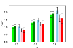
(a) 2017

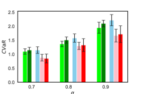
(b) 2018

(c) 2019

Figure 4: Avg. CVaR of returns across 10 portfolio trajectory simulations. Error bars report 95% CI.

   ETO-CPS     ETO-ACPS     ETO-DbS     TbS     DTbS

6.1 The portfolio optimization application

We explore the effectiveness of proposed methodologies in addressing a classic robust portfolio optimization problem. In this context, we define the cost function $c(x,\xi)$ as $-\xi^{T}x$, where $x$ represents a portfolio comprising investments in $m$ different assets, with their respective returns denoted in the random vector $\xi$. Additionally, we impose constraints on $x$, encapsulated within $\mathcal{X}$, defined as $\mathcal{X}:=\{x\in\mathbb{R}^{m}|\sum_{i=1}^{m}x_{i}=1,x\geq 0\}$. For this cost function, we obtain the partial concave conjugate function:

$$\bar{c}_{*}(x,v)=\mathop{\rm inf}_{\xi:\|\xi\|_{2}\leq R}v^{T}\xi-\xi^{T}x=-R\|v-x\|_{2}$$ (10)

Thus leading to problem 7 becoming

$$\mathop{\rm min}_{x\in\mathcal{X}}f(x,\psi):=x^{T}\mu(\psi)+\sqrt{x^{T}\Sigma(\psi)^{-1}x}$$ (11)

when $R\rightarrow\infty$, thus capturing $\Xi:=\mathbb{R}^{m}$.

6.2 CRO performance using synthetic data

We first consider a simple synthetic experiment environment where $m=2$ and where the pair $(\psi,\xi)$ is drawn from a mixture of three 4-d multivariate normal distributions. We sample N= 2000 observations and use 600 observations to train, 400 as validation, and 1000 observations for testing. All our results present statistics that are based on 10 simulations, each of which employed a slightly modified mixture model (see github repository for details). The TbS and DTbS algorithms leverage deep neural networks with the corresponding task losses to learn the necessary components ($\mu_{\theta}(\psi),\Sigma_{\theta}(\psi)$) of $\mathcal{U}_{\theta}(\psi)$. All sets are calibrated for a probability coverage of 90% and the risk of decisions is measured using CVaR at risk level $\alpha=0.9$. The average CVaR objective values and marginal coverages of the uncertainty sets can be found in the table 1. One can notice that the end-to-end based methods, TbS and DTbS significantly outperform the ETO methods on the CVaR performance. It appears that in order to maintain the required marginal coverage, the ETO approaches learned sets that resulted in overly conservative RO solutions.

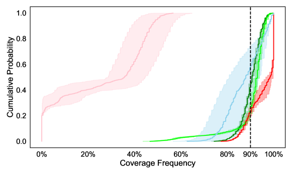
   ETO-CPS     ETO-ACPS     ETO-DbS     TbS     DTbS

Figure 5: Average cumulative distribution of conditional coverage frequency when $\psi$ is sampled uniformly from dataset over 10 simulated environments. Shaded region represent 90% CI

	CVaR	Marginal Coverage
ETO-CPS	$1.58\pm 0.03$	$91\pm 1.8\%$
ETO-ACPS	$1.69\pm 0.05$	$91\pm 1.4\%$
ETO-DbS	$1.64\pm 0.07$	$85\pm 7.8\%$
TbS	$1.03\pm 0.10$	$23\pm 6.1\%$
DTbS	$1.08\pm 0.13$	$92\pm 1.5\%$

Table 1: Avg. CVaR and marginal coverage for $\alpha=1-\epsilon=0.9$ over 10 simulated environments, error represent 90% CI.

Additionally, all the models except TbS appear to have the marginal coverage $\leavevmode\nobreak\ 90\%$ which corresponds to the $\alpha$ level they are trained for. By disregarding the aspect of coverage, TbS was able to improve on the CVaR task but suffers poorly when it comes to coverage. Comparatively, the dual task based approach DTbS was able to improve on the CVaR performance over the ETO approaches while still maintaining the necessary coverage.

As pointed out earlier, conditional coverage is a highly desirable property. Given that a synthetic environment gives us access to exact measurements of conditional coverage, figure 5 presents the cumulative distribution of the observed conditional coverage frequencies when $\psi$ is sampled uniformly from the data set. One can notice from the plot that ETO-DbS, despite being closer to required marginal coverage, failed to provide accurate conditional coverage. Among the methods that use conformality score to calibrate the radius, ETO-ACPS method which uses localized covariance matrices has better conditional coverage. However, this comes at the price of CVaR performance. The advantage of the dual task-based approach, DTbS, over the single task one are obvious. While DTbS appears to have overshot the coverage compared to ETO-ACPS, which aligns closer to 90%, we argue that this is not an issue as it ends up providing more coverage than needed while generating nearly the best average CVaR value. In figure 3c which overlays the various sets learned on the conditional distribution of $\xi$, one can notice that the sets adapt to the covariate information $\psi$ to provide the necessary conditional coverage.

6.3 CRO using US stock data

Dataset and experimental Design We follow the experimental design methodology proposed in Chenreddy et al. [2022]. Our experiments utilize historical US stock market data, comprising adjusted daily closing prices for 70 stocks across 8 sectors from January 1, 2012, to December 31, 2020, obtained via the Yahoo!Finance’s API. Each year contains 252 data points, and we calculate percentage gain/loss relative to the previous day to construct our dataset, denoted as $\xi$. We incorporate trading volume of individual stocks and other market indices as covariates. We test the robustness of all the models performance by solving the portfolio optimization problem on randomly selected stock subsets across different time spans. Utilizing 15 stocks in each window, we run the experiment ten times over three moving time frames. We maintain consistent parameters (learning rate $lr$, number of epochs $T$, step size $K$, $\gamma$). Further implementation and parameter tuning details can be found in Appendix B.3. Figure 4c compares the avg. CVaR of returns and Table 2 presents the marginal coverage across difference confidence levels for models.

It is evident from the CVaR comparison that the task based methods TbS and DTbS consistently performs better over the ETO models. Among ECRO approaches, we can clearly observe an advantage for DTbS over TbS, which has on par CVaR performance while having out of sample marginal coverage closer to the expected target level. Conformal-based ETO methods have a good marginal coverage as they are designed to have the desired coverage. Especially, ETO-ACPS and ETO-CPS, being calibrated using conformal prediction which produce statistically valid prediction regions have near target coverage levels.

Model	Year	Marginal cov. (%)
		Target $1-\epsilon$
		70%	80%	90%
ETO-CPS	2017	68	78	87
ETO-ACPS		68	77	89
ETO-DbS		54	72	85
TbS		22	26	28
DTbS		72	79	88
ETO-CPS	2018	67	79	88
ETO-ACPS		68	78	87
ETO-DbS		59	75	87
TbS		23	24	29
DTbS		71	80	93
ETO-CPS	2019	69	78	88
ETO-ACPS		71	78	89
ETO-DbS		61	76	86
TbS		26	30	32
DTbS		69	78	92

Table 2: Marginal Coverage

7 Conclusion

In summary, the paper introduces a novel framework for conditional robust optimization by combining machine learning and optimization techniques in an end-to-end approach. The study focuses on enhancing the conditional coverage of uncertainty sets and improving CRO performance. Through comparative analysis and simulated experiments, the proposed methodologies show superior results in robust portfolio optimization. The findings point to the importance of uncertainty quantification and highlight the effectiveness of an end-to-end approach in risk averse decision-making under uncertainty.

Appendix A Algorithms

Algorithm 2 Dual ECRO Training with Trust Region Solver

[1] input: dataset ${\mathcal{D}_{\psi\xi}}$, max epochs $T$, max TRO steps $K$, batch size $N$, protection level $\alpha$ Initialize a warm start buffer $\{\bar{x}_{1},\dots,\bar{x}_{M}\}$ with each $\bar{x}_{i}\in\mathcal{X}(\psi_{i})$ Initialize network parameters $\theta$ and $t=1$ not converged and ($t\leq T$) Sample a batch of $N$ indices $\mathcal{B}\subset\{1,\dots,M\}$ $i\in\mathcal{B}$ //Run TRO for up to $K$ steps $x_{i}^{t},\lambda_{i}^{t},\nu_{i}^{t}\leftarrow$ TRO($\bar{x}_{i}$, $\mu_{\theta}(\psi_{i}),\Sigma_{\theta}(\psi_{i}),K)$ $\bar{x}_{i}\leftarrow x_{i}^{t}$ Update warm start $y_{i}^{t}\leftarrow{{\bm{1}}}\{\xi_{i}\in\mathcal{E}(\mu_{\theta}(\psi_{i}),\Sigma_{\theta}(\psi_{i}))\}$ $\phi^{t}\leftarrow$ solve prob (8) for $\{(\psi_{i},y_{i}^{t})\}_{i\in\mathcal{B}}$ compute $\mathcal{L}_{DT}(\theta)$ and $\nabla_{\theta}\mathcal{L}_{DT}(\theta)$ for $i\sim\mathcal{B}$ $\theta\leftarrow\theta-\mbox{step size}\cdot\nabla_{\theta}\mathcal{L}_{DT}(\theta)$

return $\theta$

Appendix B Supplementary for Experiments

B.1 Convergence comparison

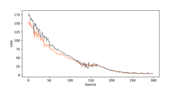
   $5$-steps TRO     TRO

Figure 6: Convergence comparison between $5$-steps TRO (46 min) and full TRO (129 min).

B.2 Synthetic conditional data generation

As we have access to the paramters of the simulation environment, we can sample the conditional multivariate Gaussian distribution of $\xi$ upon observing $\psi$ as:

$$\mu(\xi)|\psi=\bm{\mu}_{\xi}+\mathbf{\Sigma}_{\xi\psi}\cdot\mathbf{\Sigma}_{\psi\psi}^{-1}\cdot(\psi-\bm{\mu}_{\psi})$$

$$\Sigma(\xi)|\psi=\mathbf{\Sigma}_{\xi\xi}-\mathbf{\Sigma}_{\xi\psi}\cdot(\mathbf{\Sigma}_{\psi\psi})^{-1}\cdot\mathbf{\Sigma}_{\psi\xi}$$

where $\bm{\mu}_{\xi}$ is the mean vector of the dependent variables. $\bm{\mu}_{\psi}$ is the mean vector of the independent variables. $\mathbf{\Sigma}_{\xi\xi}$ is the covariance matrix of the dependent variables. $\mathbf{\Sigma}_{\xi\psi}$ is the cross-covariance matrix between dependent and independent variables. $\mathbf{\Sigma}_{\psi\psi}$ is the covariance matrix of the independent variables, and $\mathbf{\psi}$ is the observed independent variables. We sample data from these conditional distributions $\xi|\psi\sim\mathcal{N}(\mu_{\psi}(\xi),\Sigma_{\psi}(\xi))$ and compare the coverage of these observations.

B.3 Parameter tuning procedure

In this section, we explore the parameter tuning methodology applied to train the network introduced in Section 6.3. Given the time series nature of the data, we employ a rolling window technique for network training. Our architecture depends on a set of hyperparameters, defined as follows: $lr$ for learning rate, $T$ for the maximum number of epochs, $K$ for the maximum TRO steps, $B$ for the batch size, and $\alpha$ for the target level. We partition the data into training and validation periods and examine the optimal combination through grid search. For each combination, we train the network and derive the optimal policy using the training data, then applying it to the unseen validation data. The optimal combination is selected based on the lowest CVaR on the validation dataset, viewing this as a worst-case return minimization problem.

Regarding the DTbS algorithm, which balances between two losses—the CRO objective and the conditional coverage loss—we follow a specific strategy to identify the best performing model. At each epoch, we save the model and initiate model selection only after achieving the required training coverage. Subsequently, we retain the best models meeting the coverage criteria until convergence conditions are met. Among all saved models meeting the coverage requirement, we choose the one with the best CVaR objective.

B.4 Architecture

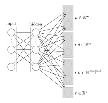
Figure 7: Example Neural Network.

References

- Amos and Kolter [2017] Brandon Amos and J Zico Kolter. Optnet: Differentiable optimization as a layer in neural networks. In International Conference on Machine Learning, pages 136–145. PMLR, 2017.
- Barber et al. [2020] Rina Barber, Emmanuel Candès, Aaditya Ramdas, and Ryan Tibshirani. The limits of distribution-free conditional predictive inference. Information and Inference: A Journal of the IMA, 10, 08 2020. doi: 10.1093/imaiai/iaaa017.
- Barratt and Boyd [2023] Shane Barratt and Stephen Boyd. Covariance prediction via convex optimization. Optimization and Engineering, 24(3):2045–2078, 2023.
- Ben-Tal and Nemirovski [1998] Aharon Ben-Tal and Arkadi Nemirovski. Robust convex optimization. Mathematics of operations research, 23(4):769–805, 1998.
- Ben-Tal et al. [2015] Aharon Ben-Tal, Dick Den Hertog, and Jean-Philippe Vial. Deriving robust counterparts of nonlinear uncertain inequalities. Mathematical programming, 149(1-2):265–299, 2015.
- Bertsimas and Kallus [2020] Dimitris Bertsimas and Nathan Kallus. From predictive to prescriptive analytics. Management Science, 66(3):1025–1044, 2020.
- Blanquero et al. [2023] Rafael Blanquero, Emilio Carrizosa, and Nuria Gómez-Vargas. Contextual uncertainty sets in robust linear optimization. 2023.
- Blondel et al. [2022] Mathieu Blondel, Quentin Berthet, Marco Cuturi, Roy Frostig, Stephan Hoyer, Felipe Llinares-López, Fabian Pedregosa, and Jean-Philippe Vert. Efficient and modular implicit differentiation. Advances in neural information processing systems, 35:5230–5242, 2022.
- Burton et al. [2020] Jason W Burton, Mari-Klara Stein, and Tina Blegind Jensen. A systematic review of algorithm aversion in augmented decision making. Journal of Behavioral Decision Making, 33(2):220–239, 2020.
- Butler and Kwon [2023] Andrew Butler and Roy H Kwon. Efficient differentiable quadratic programming layers: an admm approach. Computational Optimization and Applications, 84(2):449–476, 2023.
- Byrd et al. [2000] Richard H Byrd, Jean Charles Gilbert, and Jorge Nocedal. A trust region method based on interior point techniques for nonlinear programming. Mathematical programming, 89:149–185, 2000.
- Chenreddy et al. [2022] Abhilash Reddy Chenreddy, Nymisha Bandi, and Erick Delage. Data-driven conditional robust optimization. Advances in Neural Information Processing Systems, 35:9525–9537, 2022.
- Costa and Iyengar [2023] Giorgio Costa and Garud N Iyengar. Distributionally robust end-to-end portfolio construction. Quantitative Finance, 23(10):1465–1482, 2023.
- Donti et al. [2017] Priya Donti, Brandon Amos, and J Zico Kolter. Task-based end-to-end model learning in stochastic optimization. Advances in neural information processing systems, 30, 2017.
- Duvenaud et al. [2020] David Duvenaud, J. Zico Kolter, and Matthew Johnson. Deep implicit layers tutorial - neural ODEs, deep equilibrium models, and beyond. Neural Information Processing Systems Tutorial, 2020.
- Elmachtoub and Grigas [2022] Adam N Elmachtoub and Paul Grigas. Smart “predict, then optimize”. Management Science, 68(1):9–26, 2022.
- Gawlikowski et al. [2021] Jakob Gawlikowski, Cedrique Rovile Njieutcheu Tassi, Mohsin Ali, Jongseok Lee, Matthias Humt, Jianxiang Feng, Anna Kruspe, Rudolph Triebel, Peter Jung, Ribana Roscher, et al. A survey of uncertainty in deep neural networks. arXiv preprint arXiv:2107.03342, 2021.
- Gibbs et al. [2023] Isaac Gibbs, John J. Cherian, and Emmanuel J. Candès. Conformal prediction with conditional guarantees, 2023.
- Guo et al. [2017] Chuan Guo, Geoff Pleiss, Yu Sun, and Kilian Q Weinberger. On calibration of modern neural networks. In International conference on machine learning, pages 1321–1330. PMLR, 2017.
- Hannah et al. [2010] Lauren Hannah, Warren Powell, and David Blei. Nonparametric density estimation for stochastic optimization with an observable state variable. Advances in Neural Information Processing Systems, 23, 2010.
- Johnstone and Cox [2021] Chancellor Johnstone and Bruce Cox. Conformal uncertainty sets for robust optimization. In Conformal and Probabilistic Prediction and Applications, pages 72–90. PMLR, 2021.
- Kannan et al. [2023] Rohit Kannan, Güzin Bayraksan, and James R Luedtke. Residuals-based distributionally robust optimization with covariate information. Mathematical Programming, pages 1–57, 2023.
- Kontolati et al. [2022] Katiana Kontolati, Dimitrios Loukrezis, Dimitrios G Giovanis, Lohit Vandanapu, and Michael D Shields. A survey of unsupervised learning methods for high-dimensional uncertainty quantification in black-box-type problems. Journal of Computational Physics, 464:111313, 2022.
- Mandi et al. [2020] Jayanta Mandi, Peter J Stuckey, Tias Guns, et al. Smart predict-and-optimize for hard combinatorial optimization problems. In Proceedings of the AAAI Conference on Artificial Intelligence, volume 34, pages 1603–1610, 2020.
- Mandi et al. [2023] Jayanta Mandi, James Kotary, Senne Berden, Maxime Mulamba, Victor Bucarey, Tias Guns, and Ferdinando Fioretto. Decision-focused learning: Foundations, state of the art, benchmark and future opportunities, 2023.
- Messoudi et al. [2022] Soundouss Messoudi, Sébastien Destercke, and Sylvain Rousseau. Ellipsoidal conformal inference for multi-target regression. In Conformal and Probabilistic Prediction with Applications, pages 294–306. PMLR, 2022.
- Ohmori [2021] Shunichi Ohmori. A predictive prescription using minimum volume k-nearest neighbor enclosing ellipsoid and robust optimization. Mathematics, 9(2):119, 2021.
- Patel et al. [2023] Yash Patel, Sahana Rayan, and Ambuj Tewari. Conformal contextual robust optimization. arXiv preprint arXiv:2310.10003, 2023.
- Romano et al. [2020] Yaniv Romano, Rina Foygel Barber, Chiara Sabatti, and Emmanuel Candès. With malice toward none: Assessing uncertainty via equalized coverage. Harvard Data Science Review, 2(2):4, 2020.
- [30] Andrzej Ruszczyński and Alexander Shapiro. Chapter 6: Risk Averse Optimization, pages 223–305.
- Sadana et al. [2023] Utsav Sadana, Abhilash Chenreddy, Erick Delage, Alexandre Forel, Emma Frejinger, and Thibaut Vidal. A survey of contextual optimization methods for decision making under uncertainty. arXiv preprint arXiv:2306.10374, 2023.
- Seeger et al. [2017] Matthias Seeger, Asmus Hetzel, Zhenwen Dai, Eric Meissner, and Neil D Lawrence. Auto-differentiating linear algebra. arXiv preprint arXiv:1710.08717, 2017.
- Sen and Deng [2018] Suvrajeet Sen and Yunxiao Deng. Learning enabled optimization: Towards a fusion of statistical learning and stochastic programming. INFORMS Journal on Optimization (submitted), 2018.
- Shafer and Vovk [2008] Glenn Shafer and Vladimir Vovk. A tutorial on conformal prediction. Journal of Machine Learning Research, 9(3), 2008.
- Sun et al. [2024] Chunlin Sun, Linyu Liu, and Xiaocheng Li. Predict-then-calibrate: A new perspective of robust contextual lp. Advances in Neural Information Processing Systems, 36, 2024.
- Vovk [2012] Vladimir Vovk. Conditional validity of inductive conformal predictors. In Asian conference on machine learning, pages 475–490. PMLR, 2012.
- Wang et al. [2023] Irina Wang, Cole Becker, Bart Van Parys, and Bartolomeo Stellato. Learning for robust optimization. arXiv preprint arXiv:2305.19225, 2023.