Online Maximum Likelihood Parameter Estimation for Continuously-Monitored Quantum Systems

Abstract

In this work, we consider the problem of online (real-time, single-shot) estimation of static or slow-varying parameters along quantum trajectories in quantum dynamical systems. Based on the measurement signal of a continuously-monitored quantum system, we propose a recursive algorithm for computing the maximum likelihood estimate of unknown parameters using an approach based on stochastic gradient ascent on the log-likelihood function. We formulate the algorithm in both discrete-time and continuous-time and illustrate the performance of the algorithm through simulations of a simple two-level system undergoing homodyne measurement from which we are able to track multiple parameters simultaneously.

I Introduction

With the rapid development of engineered quantum systems, the need for estimation and monitoring of system parameters in quantum dynamical systems is an important task, e.g., when calibrating quantum experiments or for achieving high-precision sensing in quantum metrology.

In this work, we focus on the particular setting when a quantum system is subject to continuous measurements, in which case the resulting process is described by a stochastic master equation (SME), either in discrete-time via a Kraus map formulation or in continuous-time as a diffusion process [1, 2].

In the context of parameter estimation, we distinguish between two paradigms: (i) Offline or batch estimation, where the complete set of data is processed simultaneously to provide an estimate, and (ii) online or recursive estimation, where the estimate is continuously updated as new data arrives.

Among the primary motivations for studying online algorithms is the ability to track parameter changes as they happen in real-time, but online algorithms may also be useful alternatives to offline processing for very long time-series data for which the computational burden of typical offline algorithms become too heavy.

In general, the optimal parameter estimate, in the Bayesian sense, is given in terms of the solution to the (nonlinear) filtering problem (i.e., a solution to the Kushner-Stratonovich equation [3]), as sketched in [4]. In the special case where the quantum system at hand can be represented as a linear Gaussian process, the (online) parameter estimation problem can be solved by the Kalman filter as was illustrated, e.g., for a quantum harmonic oscillator subject to an unknown force [4] and for estimating a magnetic field in an atomic spin ensemble [5, 6, 7].

Except for the linear case, the filtering problem rarely has a tractable solution, but it may be approximated in various ways. For offline processing, this has been investigated via simply discretizing the parameter space [8, 9] and using Markov chain Monte Carlo methods [10, 11], whereas methods leaning towards online processing have been developed by utilizing the quantum structure to embed the discretized parameter space in an enlarged Hilbert space, resulting in the so-called quantum particle filter [12, 13, 14, 15, 16]. Common to these methods is, however, that they require propagation of a separate quantum filter for each parameter value in a discretized parameter space, resulting in very computationally demanding algorithms, especially for multi-parameter problems.

A slightly different approach is taken by [17], where classical frequency estimation techniques from the signal processing literature are employed, and in [18], where an algorithm is proposed for computing the maximum likelihood estimate without having to propagate a quantum filter.

In this work, we propose an online algorithm for computing the maximum likelihood parameter estimate with the aim of tracking slowly varying parameters. The method presented in this work relies on a recursive formulation of the gradient of the log-likelihood based on propagation of the quantum filter and the associated sensitivity equations (sometimes referred to as the filter derivative or the tangent filter). A different but commonly used method for computing the gradient of the log-likelihood is based on the smoothing distribution, typically via a forward-backward approach (see, e.g., [19]), which does not lend itself straightforwardly to a recursive formulation. By contrast, the approach based on sensitivity equations only requires integration forward in time, making it inherently recursive. For a detailed discussion on the relationship between the two approaches in the context of general hidden Markov models (HMMs), see [20, Chapter 10].

While this approach is by no means new in the context of classical systems theory (see, e.g., [21, 22]), it has received limited attention over the years. Among the latest contributions are [23], where the authors present and prove convergence of an online maximum likelihood estimator for general nonlinear diffusion processes subject to continuous-time measurements. As highlighted in [23], such methods lend themselves best to systems that admit an exact, recursive, finite-dimensional solution to the (state) filtering problem, which, in the case of uncountable state spaces, is essentially limited to linear systems and the so-called Beneš class of systems [24]. However, as it turns out, the class of stochastic quantum systems studied in the present work also admits such a solution in the form of the deceptively simple quantum filter, making them prime candidates for application of methodologies relying on such filtering solutions.

The rest of the paper is organized as follows. In Section II, we present the quantum stochastic master equation in discrete-time and derive the online maximum likelihood estimator. In Section III, we use the considerations from the discrete-time formulation to derive the continuous-time online maximum likelihood estimator. In Section IV, we demonstrate the algorithm in simulations on a simple two-level system. Lastly, in Section V, we discuss our findings and possibilities for future work.

II Discrete-Time Formulation

In the following, we will consider quantum states in the form of density operators $\rho$ on a (finite-dimensional) Hilbert space $\mathcal{H}$, i.e., $\rho\in\{\rho\in\mathcal{H}\mid\rho\geq 0,\Tr(\rho)=1\}$. Throughout the paper, we will use the tilde (~) accent to denote estimated quantities.

In the discrete-time formalism, upon observing the classical measurement $y_{k}$, the quantum state $\rho_{k}$ evolves from time $k$ to $k+1$ according to

$$\rho_{k+1} =\frac{\mathcal{K}_{y_{k},\theta}(\rho_{k})}{\Tr(\mathcal{K}_{y_{k},\theta}(\rho_{k}))}$$ (1)

with probability

$$\mathbb{P}(y_{k}=y\mid\rho_{k},\theta) =\Tr(\mathcal{K}_{y,\theta}(\rho_{k})),$$ (2)

where $\mathcal{K}_{y,\theta}(\rho)\triangleq\sum_{\mu}M^{\theta}_{y,\mu}\rho M_{y,\mu}^{\theta\dagger}$ is a partial Kraus map corresponding to measurement outcome $y$ that depends on parameter $\theta\in\mathbb{R}^{p}$. By completeness, the partial Kraus maps satisfy $\sum_{y}\Tr(\mathcal{K}_{y,\theta}(\rho))=1$.

Based on the classical measurement signal $y_{k}$, we want to recursively compute the maximum likelihood estimate $\tilde{\theta}$ of the parameter $\theta$.

II-A Maximum Likelihood Estimation

We define the (incomplete-data) likelihood function at time $T$ as

$$l_{T}(\theta;y_{T},\tilde{\rho}_{0}) \triangleq\mathbb{P}(y_{0},\dots,y_{T}\mid\theta,\tilde{\rho}_{0})$$ (3)

$$=\Tr(\mathcal{K}_{y_{T},\theta}\circ\dots\circ\mathcal{K}_{y_{0},\theta}(\tilde{\rho}_{0}))$$

$$=\prod_{k=0}^{T}\Tr(\mathcal{K}_{y_{k},\theta}(\tilde{\rho}_{k})),$$

where $\tilde{\rho}_{k}$ is the solution to the quantum filter

$$\tilde{\rho}_{k+1}=\frac{\mathcal{K}_{y_{k},\theta}(\tilde{\rho}_{k})}{\Tr(\mathcal{K}_{y_{k},\theta}(\tilde{\rho}_{k}))}.$$ (4)

From this, it is clear that we can formulate the likelihood function recursively as

$$l_{k+1}=\Tr(\mathcal{K}_{y_{k+1},\theta}(\tilde{\rho}_{k+1}))l_{k}.$$ (5)

Introducing the log-likelihood function as $\ell_{k}\triangleq\log l_{k}$, we get

$$\ell_{k+1}=\log\Tr(\mathcal{K}_{y_{k+1},\theta}(\tilde{\rho}_{k+1}))+\ell_{k}.$$ (6)

II-A1 Offline gradient ascent

A common method for finding the parameter value that maximizes the log-likelihood is via gradient ascent, i.e., by updating the parameter estimate $\tilde{\theta}$ (from some initial guess $\tilde{\theta}_{0})$ by stepping in the direction of the gradient with some (possibly varying) step size $\gamma_{i}>0$, i.e.,

$$\tilde{\theta}_{i+1}=\tilde{\theta}_{i}+\gamma_{i}\nabla_{\theta}\ell_{T}(\tilde{\theta}_{i}).$$ (7)

To be exact, the gradient $\nabla_{\theta}\ell_{T}(\tilde{\theta}_{i})$ (evaluated at the $i$’th iteration of the parameter estimate) depends on the full history of observations $y_{0},\dots,y_{T}$ at time $T$. Computing the (exact) gradient can be done in different ways, namely, via the smoothing distribution or via propagation of the so-called sensitivity equations. In this work, we only focus on the latter approach as this naturally lends itself to an eventual (approximate) online formulation.

We first note that the gradient of the log-likelihood with respect to the $p$-dimensional parameter $\theta$ can be written as

$$\nabla_{\theta}\ell_{T} =\begin{bmatrix}\mathinner{\dfrac{\partial{}\ell_{T}}{\partial{\theta_{1}}}}\\ \vdots\\ \mathinner{\dfrac{\partial{}\ell_{T}}{\partial{\theta_{p}}}}\end{bmatrix}+\sum_{k=0}^{T}\begin{bmatrix}\mathinner{\dfrac{\partial{}\ell_{T}}{\partial{\tilde{\rho}_{k}}}}\cdot\mathinner{\dfrac{\partial{}\tilde{\rho}_{k}}{\partial{\theta_{1}}}}\\ \vdots\\ \mathinner{\dfrac{\partial{}\ell_{T}}{\partial{\tilde{\rho}_{k}}}}\cdot\mathinner{\dfrac{\partial{}\tilde{\rho}_{k}}{\partial{\theta_{p}}}}\end{bmatrix},$$ (8)

where we define the filter sensitivity at time $k$ as $\xi_{j,k}\triangleq\dfrac{\partial{}\tilde{\rho}_{k}}{\partial{\theta_{j}}}$. We remark that $\xi_{j,k}$ is a traceless Hermitian operator belonging to the tangent space of density operators. For notational convenience, we will in the following only consider scalar $\theta$ and suppress the $j$-subscript, but at the end of the section, we will write the algorithm out in full for $p$-dimensional $\theta$.

Introducing the notation $\Delta\ell_{k}\triangleq\ell_{k+1}-\ell_{k}=\log\Tr(\mathcal{K}_{y_{k},\theta}(\tilde{\rho}_{k}))$, we can write the gradient recursively as

$$\nabla_{\theta}\ell_{k} =\sum_{j=0}^{k}\mathinner{\dfrac{\partial{}\Delta\ell_{j}}{\partial{\theta}}}+\mathinner{\dfrac{\partial{}\Delta\ell_{j}}{\partial{\tilde{\rho}_{j}}}}\cdot\mathinner{\dfrac{\partial{}\tilde{\rho}_{j}}{\partial{\theta}}}$$ (9)

$$=\mathinner{\dfrac{\partial{}\Delta\ell_{k}}{\partial{\theta}}}+\mathinner{\dfrac{\partial{}\Delta\ell_{k}}{\partial{\tilde{\rho}_{k}}}}\cdot\mathinner{\dfrac{\partial{}\tilde{\rho}_{k}}{\partial{\theta}}}+\nabla_{\theta}\ell_{k-1}$$

$$=\frac{\Tr(\partial_{\theta}\mathcal{K}_{y_{k},\theta}(\tilde{\rho}_{k})+\mathcal{K}_{y_{k},\theta}(\xi_{k}))}{\Tr(\mathcal{K}_{y_{k},\theta}(\tilde{\rho}_{k}))}+\nabla_{\theta}\ell_{k-1},$$

where we define the filter sensitivity at time $k$ as $\xi_{k}\triangleq\dfrac{\partial{}\tilde{\rho}_{k}}{\partial{\theta}}$, which has its own dynamics, found by differentiation of the filter evolution (4) with respect to $\theta$, i.e.,

$$\xi_{k+1} =\mathinner{\dfrac{\partial{}\left(\frac{\mathcal{K}_{y_{k},\theta}(\tilde{\rho}_{k})}{\Tr(\mathcal{K}_{y_{k},\theta}(\tilde{\rho}_{k}))}\right)}{\partial{\theta}}}+\mathinner{\dfrac{\partial{}\left(\frac{\mathcal{K}_{y_{k},\theta}(\tilde{\rho}_{k})}{\Tr(\mathcal{K}_{y_{k},\theta}(\tilde{\rho}_{k}))}\right)}{\partial{\tilde{\rho}_{k}}}}\cdot\xi_{k}$$ (10)

$$=\frac{\partial_{\theta}\mathcal{K}_{y_{k},{\theta}}(\tilde{\rho}_{k})+\mathcal{K}_{y_{k},{\theta}}(\xi_{k})}{\Tr(\mathcal{K}_{y_{k},{\theta}}(\tilde{\rho}_{k}))}$$

$$- \frac{\Tr(\partial_{\theta}\mathcal{K}_{y_{k},{\theta}}(\tilde{\rho}_{k})+\mathcal{K}_{y_{k},{\theta}}(\xi_{k}))\tfrac{\mathcal{K}_{y_{k},{\theta}}(\tilde{\rho}_{k})}{\Tr(\mathcal{K}_{y_{k},{\theta}}(\tilde{\rho}_{k}))}}{\Tr(\mathcal{K}_{y_{k},{\theta}}(\tilde{\rho}_{k}))}.$$

When these equations (i.e,. the quantum filter (4) and the filter sensitivity (10)) are simulated for a fixed parameter value $\theta$, the gradient (9) is exact and may readily be used in an offline gradient-based maximum likelihood scheme. However, due to the large computational burden of simulating these equations from time $0$ to time $T$ for each parameter update step, we seek an online approximation to the parameter update that can easily incorporate new observations as they arrive and, in particular, allow tracking of slow changes in the true, underlying parameter.

II-A2 Online gradient ascent

To make the aforementioned offline algorithm work in an online fashion, we take the following approach: Instead of simulating the entire trajectory of the filter and sensitivity equations with a fixed parameter to compute the gradient, we instead approximate the gradient by only simulating the latest recursion before updating the parameter estimate. In other words, we perform an online gradient ascent update in the form of

$$\tilde{\theta}_{k+1}=\tilde{\theta}_{k}+\gamma_{k}\nabla_{\theta}\Delta\ell_{k}(\tilde{\theta}_{k}).$$ (11)

This approach may equivalently be interpreted as simply assuming that $\ell_{k}$ in the recursion for $\ell_{k+1}$ in (6) is independent of $\theta$ and $\rho_{k}$.

To accommodate the online parameter update, the next recursion of the quantum filter and the quantum filter sensitivity will be computed using the latest parameter estimate. Hence, the full online gradient ascent algorithm can be summarized as the following set of coupled difference equations (for $\theta\in\mathbb{R}^{p}$):

$$\hat{\rho}_{k+1} =\frac{\mathcal{K}_{y_{k},\hat{\theta}_{k}}(\hat{\rho}_{k})}{\Tr(\mathcal{K}_{y_{k},\hat{\theta}_{k}}(\hat{\rho}_{k}))},$$ (12a)

$$\xi_{j,k+1} =\frac{\partial_{\theta_{j}}\mathcal{K}_{y_{k},\tilde{\theta}_{k}}(\tilde{\rho}_{k})+\mathcal{K}_{y_{k},\tilde{\theta}_{k}}(\xi_{j,k})}{\Tr(\mathcal{K}_{y_{k},\tilde{\theta}_{k}}(\tilde{\rho}_{k}))}$$

$$- \frac{\Tr(\partial_{\theta_{j}}\mathcal{K}_{y_{k},\tilde{\theta}_{k}}(\tilde{\rho}_{k})+\mathcal{K}_{y_{k},\tilde{\theta}_{k}}(\xi_{j,k}))\tfrac{\mathcal{K}_{y_{k},\tilde{\theta}_{k}}(\tilde{\rho}_{k})}{\Tr(\mathcal{K}_{y_{k},\tilde{\theta}_{k}}(\tilde{\rho}_{k}))}}{\Tr(\mathcal{K}_{y_{k},\tilde{\theta}_{k}}(\tilde{\rho}_{k}))},$$ (12b)

$$\hat{\theta}_{j,k+1} =\hat{\theta}_{j,k}+\gamma_{k}\ \frac{\Tr(\partial_{\theta_{j}}\mathcal{K}_{y_{k},\hat{\theta}_{k}}(\hat{\rho}_{k})+\mathcal{K}_{y_{k},\hat{\theta}_{k}}(\xi_{j,k}))}{\Tr(\mathcal{K}_{y_{k},\hat{\theta}_{k}}(\hat{\rho}_{k}))}$$ (12c)

for $j=1,\dots,p$.

III Continuous-time formulation

In this section, we will consider the diffusive quantum stochastic master equation given by the following stochastic differential equation (SDE), to be understood in the sense of Itô:

$$\operatorname{d\!}\rho_{t} =-i\commutator{H(\theta)}{\rho}\operatorname{d\!}t+\mathcal{D}[L]\rho_{t}\operatorname{d\!}t+\sqrt{\eta}\mathcal{H}[L](\rho_{t})\operatorname{d\!}W_{t},$$ (13a)

$$\operatorname{d\!}y_{t} =\sqrt{\eta}\Tr((L+L^{\dagger})\rho_{t})\operatorname{d\!}t+\operatorname{d\!}W_{t}$$ (13b)

with the superoperators $\mathcal{D}[L]\rho$ and $\mathcal{H}[L](\rho)$ defined as

$$\mathcal{D}[L]\rho \triangleq L\rho L^{\dagger}-\frac{1}{2}(L^{\dagger}L\rho+\rho L^{\dagger}L),$$

$$\mathcal{H}[L](\rho) \triangleq L\rho+\rho L^{\dagger}-\Tr((L+L^{\dagger})\rho)\rho.$$

Here, $H(\theta)$ (a Hermitian operator that depends on parameter $\theta$) denotes the Hamiltonian of the system. The system is subject to a continuous measurement defined in terms of the (not necessarily Hermitian) measurement operator $L$ and the measurement efficiency $\eta\in[0,1]$ with $y_{t}$ being the classical measurement signal and $W_{t}$ being a standard Wiener process. The term $\mathcal{D}[L]\rho$ corresponds to the measurement-induced decoherence. Note that the same Wiener process is driving both the process and the measurement signal—a unique feature of quantum systems—and that for $\eta=0$, the measurement signal contains no information about the quantum state. For more details on the properties of the stochastic master equation, we refer to [2] and the references therein.

For simplicity of presentation, we only consider the case where there is just a single measurement channel (with corresponding decoherence), but the model may easily be extended to the case where there are several measurement and decoherence channels. Likewise, we only consider the case where the parameter $\theta$ enters through the Hamiltonian, although we relax this assumption in the simulation examples in Section IV.

In the following, we derive an online gradient ascent algorithm in continuous-time for computing the maximum likelihood estimate $\tilde{\theta}$ of the parameter $\theta$.

With standard Itô rules (i.e., $\operatorname{d\!}W_{t}^{2}=\operatorname{d\!}t$, $\operatorname{d\!}t^{2}=0$ and $\operatorname{d\!}W_{t}\!\operatorname{d\!}t=0$), the system (13) admits the equivalent formulation

$$\rho_{t+\operatorname{d\!}t}=\frac{M_{\operatorname{d\!}y_{t}}^{\theta}\rho M_{\operatorname{d\!}y_{t}}^{\theta\dagger}+(1-\eta)L\rho_{t}L^{\dagger}\operatorname{d\!}t}{\Tr(M_{\operatorname{d\!}y_{t}}^{\theta}\rho M_{\operatorname{d\!}y_{t}}^{\theta\dagger}+(1-\eta)L\rho_{t}L^{\dagger}\operatorname{d\!}t)}$$ (14)

with $M_{\operatorname{d\!}y_{t}}^{\theta}\triangleq I-(iH(\theta)+\frac{1}{2}L^{\dagger}L)\operatorname{d\!}t+\sqrt{\eta}L\operatorname{d\!}y_{t}$, where we recognize that this a Kraus map formulation similar to (1). Writing out the partial Karus map in full, we have, still under the Itô interpretation,

$$\mathcal{K}_{\operatorname{d\!}y,\theta}(\rho) =M_{\operatorname{d\!}y}^{\theta}\rho M_{\operatorname{d\!}y}^{\theta\dagger}+(1-\eta)L\rho L^{\dagger}\operatorname{d\!}t$$ (15)

$$=\rho-i\commutator{H(\theta)}{\rho}\operatorname{d\!}t+\mathcal{D}[L]\rho\operatorname{d\!}t$$

$$\hskip 80.00012pt+\sqrt{\eta}(L\rho+\rho L^{\dagger})\operatorname{d\!}y.$$

$$\operatorname{d\!}\tilde{\rho}_{t} =\left(-i[H(\tilde{\theta}_{t}),\tilde{\rho}_{t}]+\mathcal{D}[L]\tilde{\rho}_{t}\right)\operatorname{d\!}t+\sqrt{\eta}\mathcal{H}[L](\tilde{\rho}_{t})\left(\operatorname{d\!}y_{t}-\sqrt{\eta}\Tr((L+L^{\dagger})\tilde{\rho}_{t})\operatorname{d\!}t\right)$$ (23a)

$$\operatorname{d\!}\xi_{j,t} =\left(-i\left[\partial_{\theta_{j}}H(\tilde{\theta}_{t}),\tilde{\rho}_{t}\right]-i[H(\tilde{\theta}_{t}),\xi_{j,t}]+\mathcal{D}[L]\xi_{j,t}-\eta\mathcal{H}[L](\tilde{\rho}_{t})\Tr((L+L^{\dagger})\xi_{j,t})\right)\operatorname{d\!}t$$

$$\hskip 10.00002pt+\sqrt{\eta}\left(L\xi_{j,t}+\xi_{j,t}L^{\dagger}-\left(\Tr((L+L^{\dagger})\xi_{j,t})\tilde{\rho}_{t}+\Tr((L+L^{\dagger})\tilde{\rho}_{t})\xi_{j,t}\right)\right)\left(\operatorname{d\!}y_{t}-\sqrt{\eta}\Tr((L+L^{\dagger})\tilde{\rho}_{t})\operatorname{d\!}t\right)$$ (23b)

$$\operatorname{d\!}\tilde{\theta}_{j,t} =\gamma_{t}\sqrt{\eta}\Tr((L+L^{\dagger})\xi_{j,t})\left(\operatorname{d\!}y_{t}-\sqrt{\eta}\Tr((L+L^{\dagger})\tilde{\rho}_{t})\operatorname{d\!}t\right)$$ (23c)

From (3), the likelihood function may now be written as

$$l_{t+\operatorname{d\!}t} =l_{t+\operatorname{d\!}t}(\theta;y_{t+\operatorname{d\!}t},\tilde{\rho}_{0})$$ (16)

$$=\Tr(\mathcal{K}_{\operatorname{d\!}y_{t},\theta}(\tilde{\rho}_{t}))l_{t}$$

$$=\left(1+\sqrt{\eta}\Tr((L+L^{\dagger})\tilde{\rho}_{t})\operatorname{d\!}y_{t}\right)l_{t}$$

from which the log-likelihood immediately follows to be

$$\ell_{t+\operatorname{d\!}t}=\sqrt{\eta}\Tr((L+L^{\dagger})\tilde{\rho}_{t})\\ \times\left(\operatorname{d\!}y_{t}-\frac{\sqrt{\eta}}{2}\Tr((L+L^{\dagger})\tilde{\rho}_{t})\operatorname{d\!}t\right)+\ell_{t}.$$ (17)

The full log-likelihood may then be written in integral form as

$$\ell_{t}(\theta;y_{t},\tilde{\rho}_{0})=\sqrt{\eta}\int_{0}^{t}\Tr((L+L^{\dagger})\tilde{\rho}_{s})\operatorname{d\!}y_{s}\\ -\frac{\eta}{2}\int_{0}^{t}\Tr((L+L^{\dagger})\tilde{\rho}_{s})^{2}\operatorname{d\!}s,$$ (18)

where $\tilde{\rho}_{t}$ is the solution to the quantum filter

$$\operatorname{d\!}\tilde{\rho}_{t}=-i[H({\theta}),\tilde{\rho}_{t}]\operatorname{d\!}t+\mathcal{D}[L]\tilde{\rho}_{t}\operatorname{d\!}t\\ +\sqrt{\eta}\mathcal{H}[L]\tilde{\rho}_{t}\left(\operatorname{d\!}y_{t}-\sqrt{\eta}\Tr((L+L^{\dagger})\tilde{\rho}_{t})\operatorname{d\!}t\right).$$ (19)

Following the same reasoning as in Section II-A2, we will design a continuous-time online gradient ascent update for finding the maximum likelihood parameter estimate $\tilde{\theta}$ (from some initial guess $\tilde{\theta}_{0})$. Hence, analogously to the discrete-time online parameter update (11), we have

$$\operatorname{d\!}\tilde{\theta}_{t} =\gamma_{t}\nabla_{\theta}\operatorname{d\!}\ell_{t}(\tilde{\theta}_{t})$$ (20)

$$=\gamma_{t}\nabla_{\theta}\Bigg{(}\sqrt{\eta}\Tr((L+L^{\dagger})\tilde{\rho}_{t})$$

$$\hskip 40.00006pt\times\left(\operatorname{d\!}y_{t}-\frac{\sqrt{\eta}}{2}\Tr((L+L^{\dagger})\tilde{\rho}_{t})\operatorname{d\!}t\right)\Bigg{)}$$

with $\operatorname{d\!}\ell_{t}$ denoting the integrand of (18) and $\gamma_{t}>0$ being a (possibly time-varying) learning rate. We note here that (20) may be meaningfully treated as an Itô process as $\ell_{t}$ is itself an Itô process [25].

Formally, we write the gradient of the log-likelihood with respect to the parameter $\theta$ as

$$\nabla_{\theta}\operatorname{d\!}\ell_{t}=\mathinner{\dfrac{\partial{}\operatorname{d\!}\ell_{t}}{\partial{\theta}}}+\mathinner{\dfrac{\partial{}\operatorname{d\!}\ell_{t}}{\partial{\tilde{\rho}_{t}}}}\cdot\mathinner{\dfrac{\partial{}\tilde{\rho}_{t}}{\partial{\theta}}},$$ (21)

where the filter sensitivity $\xi_{t}\triangleq\dfrac{\partial{}\tilde{\rho}_{t}}{\partial{\theta}}$ satisfies the sensitivity equation

$$\operatorname{d\!}\xi_{t}=\mathinner{\dfrac{\partial{}\operatorname{d\!}\tilde{\rho}_{t}}{\partial{\theta}}}+\mathinner{\dfrac{\partial{}\operatorname{d\!}\tilde{\rho}_{t}}{\partial{\tilde{\rho}_{t}}}}\cdot\xi_{t}$$ (22)

with $\operatorname{d\!}\tilde{\rho}_{t}$ denoting the quantum filtering equation (19). Writing out the sensitivity equation and the parameter update out in full, we get the coupled diffusion process (23) (placed at the bottom of this page).

We note here that all three equations (i.e., the quantum filter, the filter sensitivity and the parameter update) are driven by the same innovation process $\operatorname{d\!}I_{t}\triangleq\sqrt{\eta}\left(\operatorname{d\!}y_{t}-\sqrt{\eta}\Tr((L+L^{\dagger})\tilde{\rho}_{t})\operatorname{d\!}t\right)$. From this formulation, it is also clear that the learning rate $\gamma_{t}$ will directly amplify the effect of the noise inherent to the innovation process on the parameter estimate. Hence, in order for the noise to be suppressed, the learning rate must be chosen to be sufficiently slow. From a slightly different point of view, the need for a slow learning rate may also be argued as follows:

For a fixed parameter value, the innovation process must reach a steady-state distribution, which must consequently imply that both the state estimate $\tilde{\rho}_{t}$ and the filter sensitivity $\xi_{t}$ must have reached a stationary distribution, and from this stationary distribution, the gradient must be perceptible. Hence, if the change in the parameter estimate $\tilde{\theta}_{t}$ is too fast, the stochastic estimate of the gradient will not have time to stabilize and the perceived gradient will instead be dominated by random noise.

Before proceeding, we remark that the set of equations (23) could equivalently be derived directly from (12) via the Kraus map (14) and the Itô rule. We may thus interpret (12) as a (first-order) numerical integration scheme of the continuous-time online gradient ascent (23). In fact, when (23) has to be simulated, we will always recommend using the discrete-time equivalent (12) as opposed to, e.g., a naive application of the Euler-Maruyama scheme, in order to properly preserve positivity and trace of the quantum state.

IV Simulation Example

In the following, we will consider a two-level quantum system undergoing homodyne measurement, described by the stochastic master equation (13) with Hamiltonian and measurement operator given by

$$H=\frac{\Delta}{2}\sigma_{z}+\frac{\Omega}{2}\sigma_{x},\qquad L=\sqrt{\kappa}\sigma_{z},$$ (24)

where $\sigma_{j\in\{x,y,z\}}$ denotes the Pauli matrices.

This system could, for instance, represent a superconducting qubit in a rotating wave approximation, in which case $\Delta$ is the detuning between the qubit frequency and the driving field, and $\Omega$ is the Rabi frequency [26]. We typically have that these two parameters are of the same order of magnitude and much greater than the measurement rate, i.e., $\kappa\ll\mathinner{\!\left\lvert\Delta\right\rvert}$, $\mathinner{\!\left\lvert\Omega\right\rvert}$.

As discussed as the end of Section III, the learning rate $\gamma_{t}$ must be sufficiently slow compared to dynamics of the rest of the system. For the example at hand, the measurement rate $\kappa$ dictates both the rate of information extraction as well as the slowest dynamics in the system. Hence, we pick $\gamma=\frac{\kappa}{1000}$.

In the following, we will estimate all four parameters (i.e., the frequencies $\Omega$ and $\Delta$, the measurement efficiency $\eta$ and the measurement rate $\kappa$) simultaneously along a single quantum trajectory.

We consider two situations: (i) The parameters are static, but our initial estimate is wrong (see Fig. 1a), and (ii) our initial estimate is correct, but the parameters vary slowly over time (see Fig. 1b).

In the simulations, the true initial state is the ground state $\rho_{0}=\outerproduct{0}{0}$, the initial filter state is the maximally mixed state $\tilde{\rho}_{0}=\frac{1}{2}I$, and the filter sensitivities are initialized at $\xi_{j,0}=0$ for $j\in\{\Omega,\Delta,\eta,\kappa\}$. The true parameter values and the initial parameter estimates may be found from Fig. 1. The simulations are performed using the discrete-time model (12) and Kraus map (14) with a time-discretization of $\Delta t=10^{-2}$. Both simulations are run for $T=\frac{20}{\gamma}=200\cdot 10^{3}$ time units. For parameters in the MHz range, as would be typical for superconducting devices, this corresponds to 200 ms of data.

As seen from Fig. 1a, when the parameters are constant, the parameter estimates all eventually converge to the true values, although we note that $\eta$ converges significantly slower than the remaining parameters. In particular, we note that, for this specific example, the estimator for $\eta$ seems to have a behavior reminiscent of a non-minimum phase system in the sense that it initially undershoots with reference to the true value.

Likewise, when the parameters are changing slowly over time, as seen in Fig. 1b, the estimator is, to a large degree, able to track this change. A natural limitation in such tracking situations is the rate of information extraction (in this case quantified in terms of $\kappa$) and, consequently, the learning rate $\gamma$. A higher learning rate will in principle allow the estimator to react to faster changes in the parameters, but at the cost of estimation accuracy, as the larger learning rate will also amplify the unavoidable noise related to the quantum measurement process.

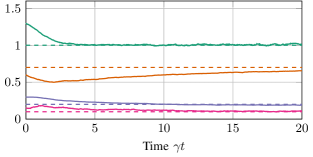
(a) Estimation of static parameters. The true parameter values (dashed lines) are $(\Omega,\eta,\Delta,\kappa)=(1,0.7,0.2,0.1)$. The estimates (solid lines) are initialized at $(\tilde{\Omega}_{0},\tilde{\eta}_{0},\tilde{\Delta}_{0},\tilde{\kappa}_{0})=(1.3,0.6,0.3,0.15)$.

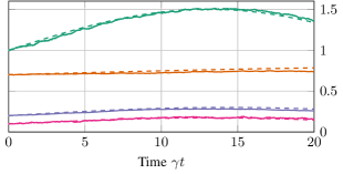
(b) Tracking of slow-varying parameters. The true parameter values (dashed lines) are given by the static parameter values from Fig. 1a plus a time-dependent perturbation $(\Omega^{\prime},\eta^{\prime},\Delta^{\prime},\kappa^{\prime})_{t}=\big{(}0.5\sin(0.12\gamma t),$ $0.2\sin(0.05\gamma t),$ $0.16\sin(0.12\gamma t),$ $0.7\sin(0.11\gamma t)\big{)}$. The estimates (solid lines) are initialized at $(\tilde{\Omega}_{0},\tilde{\eta}_{0},\tilde{\Delta}_{0},\tilde{\kappa}_{0})=(1,0.7,0.2,0.1)$.

Figure 1: Two examples of sample trajectories for the parameter estimates for the two-level quantum system described by the diffusive master equation (13) with Hamiltonian and measurement operator given by (24). The learning rate in both examples is constant and given by $\gamma=\frac{\kappa_{0}}{1000}=10^{-4}$. Simulations are done using the discrete-time model (12) and Kraus map (14) with a time-discretization of $\Delta t=10^{-2}$. The solid lines correspond to the estimated parameters, while the dashed lines correspond to the true parameter values.

V Discussion and Future Work

In this work, we have proposed an online algorithm for computing the maximum likelihood estimate of unknown parameters in a continuously-monitored quantum system and demonstrated its usefulness via a simple simulation example.

A fundamental aspect to highlight for the reason for the proposed online maximum likelihood algorithm to work is the remarkable feature of stochastic quantum systems that they admit a tractable (finite-dimensional), exact solution to the (state) filtering problem in the form of (4) and (19) for, respectively, the discrete-time and continuous-time case. Hence, in the language of nonlinear filtering theory, we may consider quantum systems as part of the class of stochastic systems that admit a tractable solution to the Kushner-Stratonovich equation.

An important next step is to formally proof convergence (in a suitable sense) of the proposed algorithm. Typically, a necessary condition for online algorithms to converge is that the underlying dynamical system, for a fixed parameter $\theta$, converges to a unique invariant measure. In our case, this would entail finding conditions under which the true quantum system $\rho_{t}$, the corresponding quantum filter $\tilde{\rho}_{t}$ and its sensitivity $\xi_{t}$ all converge to a unique invariant measure. For the quantum filter, this can be ensured under a purification condition on the measurement operators and an ergodicity condition on the Lindbladian [27, 28], whereas the sensitivity operator has yet to see any attention in the literature. We note, however, that simulations suggest that the purification condition (which automatically entails unit measurement efficiency) is overly restrictive. When such ergodicity conditions have been established, it appears reasonable to approach the convergence proof in a similar way as done by [23].

While such proofs, broadly based on stochastic approximation techniques [29], usually rely on an assumption on the learning rate $\gamma_{t}$ tending to 0 as time $t$ tends to infinity, practical applications, especially for tracking, usually requires a non-zero learning rate for all time. Hence, it is of great interest to derive bounds on the uncertainty of the parameter estimate given in terms of the magnitude of the learning rate.

As gradient descent is known to have a slow convergence rate, it might be fruitful to investigate more advanced parameter update rules such as (quasi-)Newton methods involving (approximate) second-order information or adaptive learning rates known from the (online) optimization literature [30]. This is further motivated by the presented example, where it is clear that the induced dynamics can result in undesirable properties such as an initial undershoot in some parameter estimates.

Lastly, future work may include applying the method to systems subject to jump-type measurements like photodetectors, as well as infinite-dimensional systems such as systems involving bosonic modes.

References

- [1] H. M. Wiseman and G. J. Milburn, Quantum Measurement and Control. Cambridge University Press, 2010.
- [2] P. Rouchon, “A tutorial introduction to quantum stochastic master equations based on the qubit/photon system,” Annual Reviews in Control, vol. 54, pp. 252–261, 2022.
- [3] A. H. Jazwinski, Stochastic Processes and Filtering Theory. Academic Press, 1970.
- [4] F. Verstraete, A. C. Doherty, and H. Mabuchi, “Sensitivity optimization in quantum parameter estimation,” Physical Review A, vol. 64, no. 3, p. 032111, Aug. 2001.
- [5] J. Geremia, J. K. Stockton, A. C. Doherty, and H. Mabuchi, “Quantum Kalman filtering and the Heisenberg limit in atomic magnetometry,” Physical Review Letters, vol. 91, no. 25, p. 250801, Dec. 2003.
- [6] J. K. Stockton, J. M. Geremia, A. C. Doherty, and H. Mabuchi, “Robust quantum parameter estimation: Coherent magnetometry with feedback,” Physical Review A, vol. 69, no. 3, p. 032109, Mar. 2004.
- [7] J. Amorós-Binefa and J. Kołodyński, “Noisy atomic magnetometry in real time,” New Journal of Physics, vol. 23, no. 12, p. 123030, Dec. 2021.
- [8] J. Gambetta and H. M. Wiseman, “State and dynamical parameter estimation for open quantum systems,” Physical Review A, vol. 64, no. 4, p. 042105, Sep. 2001.
- [9] P. Warszawski, J. Gambetta, and H. M. Wiseman, “Dynamical parameter estimation using realistic photodetection,” Physical Review A, vol. 69, no. 4, p. 042104, Apr. 2004.
- [10] S. Gammelmark and K. Mølmer, “Bayesian parameter inference from continuously monitored quantum systems,” Physical Review A, vol. 87, no. 3, p. 032115, Mar. 2013.
- [11] A. H. Kiilerich and K. Mølmer, “Bayesian parameter estimation by continuous homodyne detection,” Physical Review A, vol. 94, no. 3, p. 032103, Sep. 2016.
- [12] B. A. Chase and J. M. Geremia, “Single-shot parameter estimation via continuous quantum measurement,” Physical Review A, vol. 79, no. 2, p. 022314, Feb. 2009.
- [13] A. Negretti and K. Mølmer, “Estimation of classical parameters via continuous probing of complementary quantum observables,” New Journal of Physics, vol. 15, no. 12, p. 125002, Dec. 2013.
- [14] P. Six, P. Campagne-Ibarcq, L. Bretheau, B. Huard, and P. Rouchon, “Parameter estimation from measurements along quantum trajectories,” in 2015 54th IEEE Conference on Decision and Control (CDC), Dec. 2015, pp. 7742–7748.
- [15] J. F. Ralph, S. Maskell, and K. Jacobs, “Multiparameter estimation along quantum trajectories with sequential Monte Carlo methods,” Physical Review A, vol. 96, no. 5, p. 052306, Nov. 2017.
- [16] M. Bompais, N. H. Amini, and C. Pellegrini, “Parameter estimation for quantum trajectories: Convergence result,” in 2022 IEEE 61st Conference on Decision and Control (CDC), Dec. 2022, pp. 5161–5166.
- [17] J. F. Ralph, K. Jacobs, and C. D. Hill, “Frequency tracking and parameter estimation for robust quantum state estimation,” Physical Review A, vol. 84, no. 5, p. 052119, Nov. 2011.
- [18] L. Cortez, A. Chantasri, L. P. García-Pintos, J. Dressel, and A. N. Jordan, “Rapid estimation of drifting parameters in continuously measured quantum systems,” Physical Review A, vol. 95, no. 1, p. 012314, Jan. 2017.
- [19] P. Six, P. Campagne-Ibarcq, I. Dotsenko, A. Sarlette, B. Huard, and P. Rouchon, “Quantum state tomography with noninstantaneous measurements, imperfections, and decoherence,” Physical Review A, vol. 93, no. 1, p. 012109, Jan. 2016.
- [20] O. Cappé, E. Moulines, and T. Rydén, Inference in hidden Markov models, ser. Springer series in statistics. New York: Springer, 2005.
- [21] A. Benveniste, M. Métivier, and P. Priouret, Adaptive Algorithms and Stochastic Approximations. Springer Berlin Heidelberg, 1990.
- [22] L. Ljung and T. Söderström, Theory and Practice of Recursive Identification, 1st ed., ser. The MIT Press series in signal processing, optimization, and control. The MIT Pr, 1983, no. 4.
- [23] S. C. Surace and J.-P. Pfister, “Online maximum-likelihood estimation of the parameters of partially observed diffusion processes,” IEEE Transactions on Automatic Control, vol. 64, no. 7, pp. 2814–2829, Jul. 2019.
- [24] V. E. Beneš, “Exact finite-dimensional filters for certain diffusions with nonlinear drift,” Stochastics, vol. 5, no. 1-2, pp. 65–92, Jun. 1981.
- [25] R. S. Lipster and A. N. Shiryaev, Statistics of Random Processes I: General Theory, 2nd ed., ser. Stochastic Modelling and Applied Probability. Berlin Heidelberg: Springer, 2001, no. 5.
- [26] A. Blais, A. L. Grimsmo, S. Girvin, and A. Wallraff, “Circuit quantum electrodynamics,” Reviews of Modern Physics, vol. 93, no. 2, p. 025005, May 2021.
- [27] T. Benoist, M. Fraas, Y. Pautrat, and C. Pellegrini, “Invariant measure for stochastic Schrödinger equations,” Annales Henri Poincaré, vol. 22, no. 2, pp. 347–374, Feb. 2021.
- [28] T. Benoist, J.-L. Fatras, and C. Pellegrini, “Limit theorems for quantum trajectories,” Stochastic Processes and their Applications, vol. 164, pp. 288–310, Oct. 2023.
- [29] V. S. Borkar, Stochastic Approximation: A Dynamical Systems Viewpoint, 2nd ed. Singapore: Hindustan Book Agency (Springer), 2022.
- [30] E. Hazan, Introduction to Online Convex Optimization, second edition ed., ser. Adaptive Computation and Machine Learning. Cambridge, Massachusetts London, England: The MIT Press, 2022.